Exploring Adversarial Attack in Spiking Neural Networks with Spike-Compatible Gradient

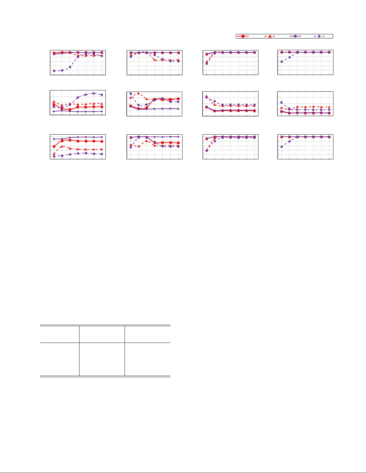
1 Exploring Adv ersarial Attack in Spiking Neural Networks with Spik e-Compatible Gradient Ling Liang, Xing Hu, Member , IEEE , Lei Deng, Member , IEEE , Y ujie W u, Guoqi Li, Member , IEEE , Y ufei Ding, Peng Li, F ellow , IEEE , Y uan Xie, F ellow , IEEE Abstract —Spiking neural network (SNN) is br oadly deployed in neuromorphic devices to emulate the brain function. In this context, SNN security becomes important while lacking in-depth in vestigation, unlike the hot wave in deep learning. T o this end, we target the adversarial attack against SNNs and identify several challenges distinct from the ANN attack: i) current adversarial attack is based on gradient information that presents in a spatio-temporal pattern in SNNs, hard to obtain with con ventional learning algorithms; ii) the continuous gradient of the input is incompatible with the binary spiking input during gradient accumulation, hindering the generation of spike-based adversarial examples; iii) the input gradient can be all-zeros (i.e. vanishing) sometimes due to the zero-dominant derivative of the ﬁring function, prone to interrupt the example update. Recently , backpropagation through time (BPTT)-inspired learning algorithms ar e widely introduced into SNNs to impro ve the perf ormance, which brings the possibility to attack the models accurately given spatio-temporal gradient maps. W e propose two approaches to address the above challenges of gradient-input incompatibility and gradient vanishing. Speciﬁcally , we design a gradient-to-spike (G2S) con verter to con vert continuous gradients to ternary ones compatible with spike inputs. Then, we design a restricted spike ﬂipper (RSF) to construct ter nary gradients that can randomly ﬂip the spike inputs with a controllable turnov er rate, when meeting all-zero gradients. Putting these methods together , we build an adversarial attack methodology for SNNs trained by supervised algorithms. Moreov er , we analyze the inﬂuence of the training loss function and the ﬁring threshold of the penultimate layer , which indicates a “trap” region under the cross-entropy loss that can be escaped by threshold tuning. Extensive experiments are conducted to validate the effectiveness of our solution, showing 99%+ attack success rate on most benchmarks, which is the best result in SNN attack. Besides the quantitative analysis of the inﬂuence factors, we evidence that SNNs ar e mor e r obust against adversarial attack than ANNs. This work can help r eveal what happens in SNN attack and might stimulate more resear ch on the security of SNN models and neuromorphic devices. K e ywor ds: Adversarial Attack, Spiking Neural Networks, Supervised Learning, Gradient Compatibility and V anishing The work was partially supported by National Science Foundation (Grant No. 1725447), Tsinghua University Initiative Scientiﬁc Research Program, Tsinghua-Foshan Innovation Special Fund (TFISF), and National Natural Science Foundation of China (Grant No. 61876215). Ling Liang and Xing Hu contributed equally to this work, corresponding author: Lei Deng. Ling Liang, Xing Hu, Lei Deng, Peng Li, and Y uan Xie are with the De- partment of Electrical and Computer Engineering, University of California, Santa Barbara, CA 93106, USA (email: { lingliang, xinghu, leideng, lip, yuanxie } @ucsb .edu). Y ujie W u and Guoqi Li are with the Department of Pre- cision Instrument, Center for Brain Inspired Computing Research, Tsinghua Univ ersity , Beijing 100084, China (email: wu-yj16@mails.tsinghua.edu.cn, liguoqi@mail.tsinghua.edu.cn). Y ufei Ding is with the Department of Com- puter Science, Univ ersity of California, Santa Barbara, CA 93106, USA (email: yufeiding@cs.ucsb.edu). I . I N T RO D U C T I O N Spiking neural networks (SNNs) [1] closely mimic the behaviors of neural circuits via spatio-temporal neuronal dy- namics and event-dri ve activities (1-spike or 0-nothing). They hav e shown promising ability in processing dynamic and noisy information with high efﬁciency [2], [3] and hav e been applied in a broad spectrum of tasks such as optical ﬂo w estimation [4], spike pattern recognition [5], SLAM [6], probabilistic in- ference [3], heuristically solving NP-hard problem [7], quickly solving optimization problem [8], sparse representation [9], robotics [10], and so forth. Besides the algorithm research, SNNs are widely deployed in neuromorphic devices for low- power brain-inspired computing [8], [11]–[13]. W ith more attention on SNNs from both academia and industry , the security problem becomes quite important. Here we focus on adversarial attack [14], one of the most popular threat models for neural network security . In adv ersarial attack, the attacker introduces imperceptible malicious perturbation into the input data, i.e. generating adversarial examples, to manipulate the model to cross the decision boundary thus misleading the classiﬁcation result. Usually , there are two categories of approach to realize adversarial attack: content- based and gradient-based. The former directly modiﬁes the semantic information (e.g. brightness, rotation, etc.) of inputs or injects predeﬁned T rojan into inputs [15]–[19]; while the latter modiﬁes inputs according to the input gradient under speciﬁed labels [20]–[24]. The gradient-based adversarial at- tack is able to achiev e a better attack ef fectiv eness, which is the focus of this work. Although adversarial attack is a very hot topic in artiﬁcial neural networks (ANNs), it is rarely studied in the SNN domain. W e identify several challenges in attacking an SNN model using adversarial examples. First, the input gradient in SNNs presents as a spatio-temporal pattern that is hard to obtain with traditional learning algorithms like the gradient- free unsupervised learning [25], [26] and spatial-gradient-only ANN-to-SNN-con version learning [27]. Second, the gradients are continuous v alues, incompatible with the binary spiking in- puts. This data format incompatibility impedes the generation of spik e-based adv ersarial examples via gradient accumulation. At last, there is sev ere gradient vanishing when the gradient crosses the step ﬁring function with a zero-dominant deri va- tiv e, which will interrupt the update of adversarial examples. In fact, there are se veral prior studies on SNN attack using trial-and-error input perturbation or transferring the techniques proposed for ANN attack. Speciﬁcally , the input can be 2 perturbed in a trial-and-error manner by simply monitoring the output change without calculating the gradient [28], [29]; the adv ersarial e xamples generated by the substitute ANN counterpart can be inherited to attack the SNN model [30]. Howe v er , they just circumvent rather than directly solve the SNN attack problem, which leads to some drawbacks that will ev entually lower down the attack ef fectiv eness. For example, the trial-and-error input perturbation method faces a large search space without the guidance of supervised gradients; the SNN/ANN model con version method needs extra model transformation and ignores the gradient information in the temporal dimension. Recently , the backpropagation through time (BPTT)- inspired supervised learning algorithms [2], [5], [31]–[35] are widely introduced into SNNs for performance boost, which enables the direct acquisition of gradient information in both spatial and temporal dimensions, i.e. spatio-temporal gradient map. This brings opportunity to realize an accurate SNN attack based on spatio-temporal input gradients directly calculated in SNNs without model conv ersion. Then, to address the men- tioned issues of gradient-input incompatibility and gradient vanishing, we propose two approaches. W e design a gradient- to-spike (G2S) con v erter to con vert continuous gradients to ternary ones that are compatible with spike inputs. G2S exploits smart techniques including probabilistic sampling, sign extraction, and overﬂo w-aware transformation, which can simultaneously maintain the spik e format and control the perturbation magnitude. Then we design a restricted spik e ﬂipper (RSF) to construct ternary gradients that can randomly ﬂip the spike inputs when facing all-zero gradient maps, where the turnov er rate of inputs is controllable. Under this attack methodology for both untargeted and targeted attacks, we analyze the impact of two important factors on the attack effecti v eness: the format of training loss function and the ﬁring threshold. W e ﬁnd a “trap” region for the model trained by cross-entropy (CE) loss, which makes it harder to attack when compared to the one trained by mean square error (MSE) loss. Fortunately , the “trap” region can be escaped by adjusting the ﬁring threshold of the penultimate layer . W e extensi vely validate our SNN attack methodology on both neuromorphic datasets (e.g. N-MNIST [36] and CIF AR10- D VS [37]) and image datasets (e.g. MNIST [38] and CIF AR10 [39]), and achieve superior attack results. W e summarize our contributions as belo w: • W e identify the challenges of adversarial attack against SNN models, which are quite different from the ANN attack. Then, we realize accurate SNN attack for the ﬁrst time via spike-compatible spatio-temporal gradient. This work can help reveal what happens in attacking SNNs and might stimulate more research on the security of SNN models and neuromorphic devices. • W e design a gradient-to-spike (G2S) con verter to ad- dress the gradient-input incompatibility problem and a restricted spike ﬂipper (RSF) to address the gradient van- ishing problem, which form a gradient-based adversarial attack methodology against SNNs trained by supervised algorithms. The perturbation magnitude is well controlled in our design. • W e explore the inﬂuence of the training loss function and the ﬁring threshold of the penultimate layer , and propose threshold tuning to improve the attack ef fectiv eness. • Extensive experiments are conducted on both neuromor- phic and image datasets, where our methodology shows 99%+ attack success rate in most cases, which is the best result on SNN attack. Besides, we demonstrate the higher robustness of SNNs against adv ersarial attack when compared with ANNs. The rest of this paper is organized as follows: Section II provides some preliminaries of SNNs and adversarial attack; Section III discusses the challenges in SNN attack and our differences with prior work; Section IV and Section V il- lustrate our attack methodology and the two factors that can affect the attack effecti veness; The e xperimental setup and the result analyses are shown in Section VI; Finally , Section VII concludes and discusses the paper . I I . P R E L I M I NA R I E S A. Spiking Neural Networks Inspired by the biological neural circuits, SNN is designed to mimic their behaviors. A spiking neuron is the basic structural unit, as sho wn in Figure 1, which is comprised of dendrite, soma and axon; many spiking neurons connected by weighted synapses form an SNN, in which the binary spike events carry information for inter-neuron communica- tion. Dendrite integrates the weighted pre-synaptic inputs, and soma consequently updates the membrane potential and determines whether to ﬁre a spike or not. When the membrane potential crosses a threshold, a spike will be ﬁred and sent to post-neurons through axon. t s o m a d e n d r it e a x o n s y n a p s e t s o m a d e n d r it e a x o n s y n a p s e 1 1 1 1 1 0 0 0 0 0 1 0 0 1 0 1 t t t 0 1 0 1 1 0 0 0 ( a )           ( b )           ( t )   Figure 1: Introduction of SNNs: (a) neuronal components; (b) computing model. The leaky integrate-and-ﬁre (LIF) model [40] is the most widely adopted SNN model. The beha vior of each LIF neuron can be brieﬂy expressed as      τ du ( t ) dt = − u ( t ) + P j w j o j ( t ) ( o ( t ) = 1 & u ( t ) = u 0 , if u ( t ) ≥ u th o ( t ) = 0 , if u ( t ) < u th (1) where t denotes the time step, τ is a time constant, and u and o represent the membrane potential and resulting output 3 spike, respectiv ely . w j is the synaptic weight between the j - th pre-neuron and the current neuron, and o j is the output spike of the j -th pre-neuron (also as the input spike of the current neuron). u th is the mentioned ﬁring threshold and u 0 is the reset potential used after ﬁring a spike. Note that a spik e should be modeled as the Dirac delta function in the continuous time domain; otherwise, it cannot increase the potential. The network structure of feedforward SNNs can be similar with that of ANNs, including conv olutional (Con v) layer , pool- ing layer , and fully-connected (FC) layer . The network inputs can be spike events captured by dynamic vision sensors [41] (i.e. neuromorphic datasets) or con verted from normal image datasets through Bernoulli sampling [2]. The classiﬁcation is conducted based on the spikes of the output layer . B. Gradient-based Adversarial Attac k W e take the gradient-based adversarial attack in ANNs as an illustrative example. The neural network is actually a map from inputs to outputs, i.e. y = f ( x ) , where x and y denote inputs and outputs, respecti vely , and f : R m → R n is the map function. Usually , the inputs are static images in conv olutional neural networks (CNNs). In adversarial attack, the attacker attempts to manipulate the victim model to produce incorrect outputs by adding imperceptible perturbations δ in the input images. W e deﬁne x 0 = x + δ as an adversarial example. The perturbation is constrained by k δ k p = k x 0 − x k p ≤  , where k·k p denotes the p -norm and  reﬂects the maximum tolerable perturbation. Generally , the adversarial attack can be cate gorized into untargeted attack and targeted attack according to the different attack goals. Untargeted attack fools the model to classify the adversarial example into any other class except for the original correct one, which can be illustrated as f ( x + δ ) 6 = f ( x ) . In contrast, for targeted attack, the adversarial example must be classiﬁed in to a speciﬁed class, i.e. f ( x + δ ) = y targ et . W ith these preliminary knowledge, the adversarial attack can be formulated as an optimization problem as belo w to search the smallest perturbation:    arg min δ k δ k p , s.t. f ( x + δ ) 6 = f ( x ) , if untargeted arg min δ k δ k p , s.t. f ( x + δ ) = y targ et , if targeted . (2) There are sev eral widely-adopted adversarial attack algo- rithms to ﬁnd an approximated solution of the above opti- mization problem. Here we introduce two of them: the fast gradient sign method (FGSM) [20] and the basic iterati ve method (BIM) [21]. FGSM . The main idea of FGSM is to generate the adversarial examples based on the gradient information of the input. Speciﬁcally , it calculates the gradient map of an input image, and then adds or subtracts the sig n of this input gradient map in the original image with multiplying a small scaling factor . The generation of adversarial examples can be formulated as ( x 0 = x + η · sig n ( O x L ( θ , x, y org inal )) , if untargeted x 0 = x − η · sig n ( O x L ( θ , x, y targ et )) , if targeted (3) where L and θ denote the loss function and parameters of the victim model. η is used to control the magnitude of the perturbation, which is usually small. In untargeted attack, the adversarial example will driv e the output aw ay from the original correct class, which results from the gradient ascent- based input modiﬁcation; while in targeted attack, the output under the adversarial example goes tow ards the targeted class, owing to the gradient descent-based input modiﬁcation. BIM . BIM algorithm is actually the iterativ e version of the abov e FGSM, which updates the adversarial examples in an iterativ e manner until the attack succeeds. The generation of adversarial examples in BIM is gov erned by ( x 0 k +1 = x 0 k + η · sig n ( O x 0 k L ( θ , x 0 k , y org inal )) , if untargeted x 0 k +1 = x 0 k − η · sig n ( O x 0 k L ( θ , x 0 k , y targ et )) , if targeted (4) where k is the iteration inde x. Speciﬁcally , x 0 k equals the original input when k = 0 , i.e. x 0 0 . In ANNs, sev eral adv anced attack methods can be poten- tially extended beyond BIM based algorithm by optimizing the perturbation bound [19], [22]–[24] or avoiding the gradient calculation [15]–[18]. In this work, we aim at the preliminary exploration of an effecti ve gradient-based SNN attack, thus adopting the most classic BIM algorithm in our design. W e leav e the SNN attack with different approaches in future work. I I I . C H A L L E N G E S I N S N N A T TAC K Even though the attack methodology can be independent of how the model is trained (e.g., gradient-free unsupervised learning [42] or gradient-based supervised learning [30]) and it is not necessary to compute gradients when ﬁnding ad- versarial examples (e.g., using trial-and-error methods [28], [29]), we take SNN models trained by BPTT with high recognition accuracy for example and focus on the spatio- temporal gradient based attack due to the potential for high attack success rate. Therefore, all our following discussions about the challenges are restricted in this context. Figure 2(a) brieﬂy illustrates the work ﬂo w of adversarial attack based on gradients. There are three stages: forward pass to obtain the model prediction, backward pass to calculate the input gradient, and input update to generate the adversarial example. This ﬂow is straightforward to implement in ANNs, as shown in Figure 2(b), which is very similar to the ANN training. The only difference lies in the input update that replaces the parameter update in a normal ANN training. Howe v er , the case becomes complicated in the SNN scenario, where the processing is based on binary spikes with temporal dynamics rather than continuous activ ations with immediate response. According to Figure 2(c), we attempt to identify the challenges in SNN attack to distinguish from the ANN attack and compare our solution with prior studies in the following subsections. 4 Sa m p l e Input F orw a rd P ropa g a t i o n L os s O u t put & L a bel Inp ut G ra di e nt                            x i xs B a ck w a rd P ropa g a t i o n + G r a d i e n t B a se d A tt a c k A r ti f i c i a l N e u r a l N e tw o r k ( A N N ) Sp i k i n g N e u r a l N e tw o r k ( S N N ) (a ) (b) ( c) t - 1 , t , t +1 • G ra d i e n t A c q u i ri n g • G ra d i e n t Fo rm a t • G ra d i e n t Va n i s h i n g C h a l l e n ges Figure 2: Illustration of gradient-based adversarial attack: (a) overall ﬂow including forward pass, backward pass, and input update; (b) adversarial attack in ANNs; (c) adversarial attack in SNNs and its challenges. xi and xs represent an input in image and spike formats, respecti vely . A. Challenges and Solutions Acquiring Spatio-temporal Gradients. In feedforward ANNs, both the activations and gradients in volve only the spatial dimension without temporal components. For each feature map, its gradient during the backward propagation is still in a 2D shape. Whereas, each gradient map becomes 3D in SNNs due to the additional temporal dimension. It is dif ﬁcult to acquire the spatio-temporal gradients using con ventional SNN learning algorithms for the generation of adversarial examples with both spatial and temporal components. F or example, the unsupervised learning rules such as spike timing dependent plasticity (STDP) [25] update synapses according to the acti vities of local neurons, which cannot help calculate the input gradients. The ANN-to-SNN-con version learning methods [27] simply con vert an SNN learning problem into an ANN one with only spatial information, leading to the incapability in capturing temporal input gradients. Recently , the backpropagation through time (BPTT)-inspired learning algorithm [2], [5], [31]–[34] is broadly studied to improve the accuracy of SNNs. This emerging supervised learning promises accurate SNN attack via the direct acquisition of input gradients in both spatial and temporal dimensions, which is adopted by us. Incompatible Format between Gradients and Inputs. The input gradients are in continuous v alues, while the SNN inputs are in binary spikes (see the left of Figure 2(c), each point represents a spike event, i.e. “1”; otherwise it is “0”). This data format incompatibility impedes the generation of spike- based adversarial examples if we consider the conv entional gradient accumulation. In this work, we propose a gradient-to- spike (G2S) con verter to con v ert continuous gradients to spik e- compatible ternary gradients. This design exploits probabilistic sampling, sign extraction, and ov erﬂow-a ware transformation, which can simultaneously maintain the spike format and control the perturbation magnitude. Gradient V anishing Problem. The thresholded spike ﬁring of the LIF neuron, as mentioned in Equation (1), is actually a step function that is non-dif ferentiable. T o address this issue, a Dirac-like function is introduced to approximate the deriv ativ e of the ﬁring activity [31]. Ho wev er , this approximation brings abundant zero gradients outside the gradient window (to be shown latter), leading to sev ere gradient vanishing during backpropagation. W e ﬁnd that the input gradient map can be all-zero sometimes, which interrupts the gradient-based update of adversarial examples. T o this end, we propose a restricted spike ﬂipper (RSF) to construct ternary gradients that can randomly ﬂip the binary inputs in the case of all- zero gradients. W e use a baseline sampling factor to bound the overall turnov er rate, making the perturbation magnitude controllable. B. Comparison with Prior W ork on SNN Attack The study on SNN attack is rarely seen, which is still in its infant stage. W e only ﬁnd several related works talking about this topic. In this subsection, we summarize their approaches and clarify our differences compared with them. T rial-and-Error Input Perturbation. Such attack algorithms perturb inputs in a trial-and-error manner by monitoring the variation of outputs. For example, A. Marchisio et al. [28] modify the original image inputs before spike sampling. They ﬁrst select a block of pix els in the images, and then add a pos- itiv e or negati ve unit perturbation onto each pixel. During this process, they always monitor the output change to determine the perturbation until the attack succeeds or the perturbation exceeds a threshold. Ho wev er , this image-based perturbation is not suitable for the data sources with only spike events [36], [37]. In contrast, A. Bagheri et al. [29] directly perturb the spike inputs rather than the original image inputs. The main idea is to ﬂip the input spikes and also monitor the outputs. SNN/ANN Model Con version. S. Sharmin et al. [30] con vert the SNN attack problem into an ANN one. They ﬁrst build an ANN substitute model that has the same network structure and parameters copied from the trained SNN model. The gradient- based adversarial attack is then conducted on the built ANN counterpart to generate the adversarial examples. 5 T able I: Comparison with prior work on SNN attack. Attack Method Data Source Spatio-temporal Gradient Computational Complexity Attack Effectiveness Trial-and-Error [28] Image % I ter × N × 2 C F P Low Trial-and-Error [29] Spike % I ter × N × C F P Low Model Conv ersion [30] Image % I ter × ( C F P + C BP ) Low This W ork Spike/Image ! I ter × ( C F P + C BP ) High These existing works suffer from sev eral drawbacks that would e ventually degrade the attack ef fectiv eness. For the trial-and-error input perturbation methods, the computational complexity is quite high due to the large search space with- out the guidance of supervised gradients. Speciﬁcally , each selected element of the inputs needs to run the forward pass once (for spike perturbation) or twice (for image perturbation) to monitor the outputs. The total computational complexity is I te r × N × C F P , where I ter is the number of attack iterations, N represents the size of search space, and C F P is the computational cost of each forward pass. This complexity is much higher than the normal one, i.e. I ter × ( C F P + C B P ) , due to the large N . Because it is difﬁcult to ﬁnd the optimal perturbation in such a huge space, the attack ef fecti veness cannot be satisfactory gi ven a limited search time in reality . Regarding the SNN/ANN model con version method, an extra model transformation is needed and the temporal information is lost during the SNN-to-ANN con version. Using a differ - ent model to ﬁnd gradients and the missing of temporal components will compromise the attack effecti veness in the end. Moreover , this method is not applicable to the image- free spiking data sources without the help of extra signal con version. Compared with the above works we calculate the gradients in both spatial and temporal dimensions without extra model con version, which matches the natural SNN behaviors. As a result, the spatio-temporal input gradients can be acquired in a supervised manner , laying a foundation for effecti ve attack. Then, the proposed G2S and RSF enable the generation of spiking adversarial examples based on the continuous gradients e ven if when meeting the gradient vanishing. This direct generation of spiking adversarial examples makes our methodology suitable for the image-free spiking data sources. For the SNN models using image-based data sources, our solution is also applicable with a simple temporal aggregation of spatio-temporal gradients. In summary , T able I sho ws the differences between our work and prior work. The attack ef- fectiv eness in the table is a joint indicator of the computational complexity , compatibility of input data formats, and attack success rate (under the same restriction of perturbation bound). If a method can achieve high attack success rate with relativ e low complexity and better compatibility of input data formats, we think it has high ef fectiv eness. Please note that we focus on the white-box attack in this paper . Speciﬁcally , in the white-box attack scenario, the adversary knows the network structure and model parameters (e.g. weights, u th , etc.) of the victim model. The reason of this scenario selection lies in that the white-box attack is the fundamental step to understand adversarial attack, which is more appropriate for the preliminary exploration on the direct adversarial attack against SNNs based on accurate gradients. Furthermore, the methodology built for the white-box attack can be easily transferred to the black-box attack in the future. I V . A DV E R S A R I A L A T TAC K S A G A I N S T S N N S In this section, we ﬁrst introduce the input data format brieﬂy , and then explain the ﬂo w , approach, and algorithm of our attack methodology in detail. Input Data Format. It is natural for an SNN model to handle spike signals. Therefore, considering the datasets containing spike e vents, such as N-MNIST [36] and CIF AR10- D VS [37], is the ﬁrst choice. In this case, the input is originally in a spatio-temporal pattern with a binary value for each element (0-nothing; 1-spike). The attacker can ﬂip the state of selected elements, while the binary format must be maintained. Due to the lack of spiking data sources in reality , the image datasets are also widely used in the SNN ﬁeld by conv erting them into the spiking version. There are different ways to perform the data conv ersion, such as rate coding [2], [5], [43] and latency coding [44]–[46]. In this work, we adopt the former scheme based on Bernoulli sampling that con verts the pixel intensity to a spike train (recalling the “Sample” in Figure 2), where the spike rate is proportional to the intensity value. In this case, the attacker can modify the intensity value of selected pix els by adding the continuous perturbation. Figure 3 illustrates the adversarial e xamples in these tw o cases. Im a ge In p u t S p i k i n g In p u t O r i gi n a l In p u t A d v er s a r i a l In p u t Cl a s s i f i ed a s ‘ 3 ’ Cl a s s i f i e d a s ‘ 8 ’ A ggr e ga t e d S p i k i n g In p u t Figure 3: The data format of original inputs and adversarial examples. The red and blue colors denote two spike channels induced by dynamic vision sensors [36], [41]. A. Attack Flow Overview The overvie w of the proposed adversarial attack against SNNs is illustrated in Figure 4. The basic ﬂo w adopts the BIM method given in Equation (4), which is the result after considering the spiking inputs of SNNs. The perturbation for 6 L o s s ( M S E / CE ) E x i s t N o n - Zero G r a d i en t G r a d i en t - to - S p i k e Co n v ert er Y es No S p i k i n g In p u t Im a ge In p u t BP FP Sa m p l e A g g r e g a te 󰪦 󰪧 󰪨 R e s t r i c t e d S p i k e F l i p p er Figure 4: Overview of the adversarial attack ﬂow for SNNs with spiking inputs or image inputs. The attack ﬂow consists of: 1  calculating continuous spatio-temporal input gradients via BPTT ; 2  generating spike-compatible input gradients; 3  updating adversarial examples. For image-based inputs, an additional aggregation of the input gradients along the temporal dimension is needed. spikes can only ﬂip the binary states (0 or 1) of selected input elements rather than add continuous values. Therefore, to generate spiking adversarial examples that are able to cross the decision boundary , the search of candidate elements is more important than the perturbation magnitude. FGSM cannot do this since it only explores the perturbation magnitude, while BIM realizes this by searching new candidate elements in different iterations. As aforementioned, there are three stages: forward pass (FP), backward pass (BP), and input update, which is executed iterativ ely until the attack succeeds. The gradients here are in a spatio-temporal pattern, which matches the spatio-temporal dynamics of SNNs and enables a higher attack effecti veness. Besides, the incompatibility between continuous gradients and binary inputs is addressed by the proposed gradient-to-spike (G2S) conv erter; the gradient vanishing problem is solved by the proposed restricted spike ﬂipper (RSF). Next, we describe the speciﬁc ﬂow for spiking inputs and image inputs individually for a clear understanding. Spiking Inputs. The blue arrows in Figure 4 illustrate this case. The generation of spiking adversarial examples relies on three steps as follo ws. In step 1  , the continuous gradients are calculated in the FP and BP stages by ( δ s 0 k = O xs 0 k L ( θ , xs k , y orig inal ) , if untargeted δ s 0 k = − O xs 0 k L ( θ , xs k , y targ et ) , if targeted (5) where δ s 0 k represents the input gradient map at the k -th iteration. Since all elements in δ s 0 k are continuous values, they cannot be directly accumulated onto the spiking inputs (i.e. xs k ) to av oid breaking the data format of binary spikes. Therefore, in the step 2  , we propose G2S conv erter to conv ert the continuous gradient map to a ternary one compatible with the spike input, which can simultaneously maintain the input data format and control the perturbation magnitude. When the input gradient vanishes (i.e. all elements in δ s 0 k are zero), we propose RSF to construct a ternary gradient map that can randomly ﬂip the input spikes with a controllable turnover rate. At last, step 3  accumulates the ternary gradients onto the spiking input. Image Inputs. Sometimes, the benchmarking models conv ert image datasets to spike inputs via Bernoulli sampling. In this case, one more step is additionally needed to generate image- style adversarial examples, which is shown by the red arro ws in Figure 4. After the above step 2  , the ternary gradient map should be aggregated in the temporal dimension, i.e. a veraging all elements belonging to the same spatial location but in different timesteps, according to δ i k = 1 T P T t =1 δ s t k . After this temporal aggregation, the image-compatible input perturbation can be acquired. In each update iteration, the intensity value of xi k will be clipped within [0 , 1] . Note that, although our method aggregates the gradients from all timesteps in this scenario, the gradient at every timestep is directly found in the target SNN model, which can be more accurate than those found by prior approaches. B. Acquisition of Spatio-T emporal Gradients W e introduce the state-of-the-art supervised learning algo- rithms for SNNs [5], [31], [33], which are inspired by the backpropagation through time (BPTT) to acquire the gradients in both spatial and temporal dimensions. Here we take the one in [5] as an illustrative example. In order to simulate in current programming frameworks (e.g. Pytorch), the original LIF neuron model in Equation (1) should be ﬁrst con verted to its equi valent iterativ e version. Speciﬁcally , we hav e ( u t +1 ,n +1 i = e − dt τ u t,n +1 i (1 − o t,n +1 i ) + P j w n ij o t +1 ,n j o t +1 ,n +1 i = f ir e ( u t +1 ,n +1 i − u th ) (6) where t and n represent indices of the simulation time step and the layer , respectiv ely , dt is the time step length, and e − dt τ reﬂects the leakage effect of the membrane potential. f ire ( · ) is a step function, which satisﬁes f ir e ( x ) = 1 when x ≥ 0 , otherwise f ir e ( x ) = 0 . This iterativ e LIF model incorporates all behaviors of a spiking neuron, including integration, ﬁre, and reset. Note that a spike can be simply modeled as a binary ev ent (1 or 0) in the abov e discrete time domain, which differs from that in the continuous time domain in Equation (1). In the output layer , we adopt the commonly-used spike rate coding scheme for the recognition, i.e., the neuron ﬁring the most spikes becomes the winner that indicates the class prediction. The spatio-temporal spike pattern of the output 7 layer is conv erted into a spike rate vector , described as y i = 1 T T X t =1 o t,N i (7) where N is the output layer index and T is the length of the simulation time windo w . This spike rate vector can be regarded as the normal output vector in ANNs. With this output con version, the typical loss functions L for ANNs, such as mean square error (MSE) and cross-entropy (CE), can also be applied in the loss function for SNNs. Based on the iterativ e LIF neuron model and a gi ven loss function, the gradient propagation can be governed by      ∂ L ∂ o t,n i = P j ∂ L ∂ u t,n +1 j ∂ u t,n +1 j ∂ o t,n i + ∂ L ∂ u t +1 ,n i ∂ u t +1 ,n i ∂ o t,n i ∂ L ∂ u t,n i = ∂ L ∂ o t,n i ∂ o t,n i ∂ u t,n i + ∂ L ∂ u t +1 ,n i ∂ u t +1 ,n i ∂ u t,n i . (8) Howe v er , the ﬁring function is non-dif ferentiable, i.e. ∂ o ∂ u does not exist. As mentioned earlier, a Dirac-like function is introduced to approximate its deriv ati ve [31]. Speciﬁcally , ∂ o ∂ u can be estimated by ∂ o ∂ u ≈ ( 1 a , | u − u th | ≤ a 2 0 , other w ise (9) where a is a hyper-parameter to control the gradient width when passing the ﬁring function during backpropagation. This approximation indicates that only the neurons whose membrane potential is close to the ﬁring threshold have the chance to let gradients pass through, as shown in Figure 5. It can be seen that abundant zero gradients are produced, which might lead to the gradient vanishing problem (all input gradients become zero). 0.1 0.0 0.1 Value 1 0 2 1 0 0 1 0 2 1 0 4 #Elements Class0 Class1 Class2 Class3 Class4 Class5 Class6 Class7 Class8 Class9 Figure 5: The distribution of input gradients ov erall 500 samples from N-MNIST . The model is trained with MSE loss. Most of gradients are zero which might lead to the gradient vanishing problem. During the adversarial attack, we consider the attack is successful when the adversarial example can fool the SNN model still under the spike rate coding scheme, i.e., letting any other neuron ﬁre the most spikes (untargeted attack) or letting the tar geted neuron ﬁre the most spikes (targeted attack). C. Gradient-to-Spik e (G2S) Con verter There are two goals in the design of G2S conv erter in each iteration: (1) the ﬁnal gradients should be compatible with the spiking inputs, i.e. remaining the spike format unchanged after the gradient accumulation; (2) the perturbation magnitude should be imperceptible, i.e. limiting the number of non-zero gradients. T o this end, we design three steps: probabilistic sampling, sign extraction, and ov erﬂow-a ware transformation, which are illustrated in Figure 6.     󰇛     󰆒  󰇜 0 0 1 1 0 1 1 . 0 0 . 4 0 .1 0 0 .7 0 . 8 1 . 0 0 . 4 0 .1 0 0 .7 0 . 8 - 2 .0 0 .8 - 0 .2 0 1 .4 - 1 .6 - 2 .0 0 .8 - 0 .2 0 1 .4 - 1 .6 1 1 0 0 0 1 1 1 0 0 0 1 - 1 1 0 0 0 - 1 - 1 1 0 0 0 - 1 0 1 0 0 0 - 1 0 1 0 0 0 - 1 S i g n N o r m T r a n s f o r m    󰆒        S a m p l e    󰇛   󰆒       󰇜    󰆒 Figure 6: Illustration of gradient-to-spike (G2S) con v erter with probabilistic sampling reducing the number of modiﬁed points and thus lowering the perturbation magnitude, sign extraction ternarizing the continuous gradients for spike compatibility , and ov erﬂow-a ware transformation clipping the data range in adversarial examples. Probabilistic Sampling. The absolute value of the input gradient map obtained by Equation (5), i.e. | δ s 0 k | , is ﬁrst normalized to lie in the range of [0 , 1] . Then, the normalized gradient map, i.e. nor m ( | δ s 0 k | ) , is sampled to produce a binary mask with the same shape, in which the 1s indicate the locations where gradients can pass through. The probabilistic sampling for each gradient element obeys ( P ( δ mask = 1) = nor m ( | δ s 0 k | ) P ( δ mask = 0) = 1 − nor m ( | δ s 0 k | ) . (10) In other words, a larger gradient has a larger possibility to let the gradient pass through. By multiplying the resulting mask with the original gradient map, the number of non- zero elements can be reduced signiﬁcantly . T o evidence this conclusion, we run the attack against the SNN model with a network structure to be provided in T able V ov er 500 spiking inputs from N-MNIST , and the results are presented in Figure 7. Giv en MSE loss and untarget attack scenario, the number of non-zero elements in δ s 0 k could reach 2 10 . After using the probabilistic sampling, the number of non-zero elements in δ s 0 k  δ mask can be greatly decreased, masking out > 96% percentage. Sign Extraction. Now , we explain ho w to generate a ternary gradient map where each element is in {− 1 , 0 , 1 } , which can maintain the spike format after accumulating onto the spiking inputs with binary values of { 0 , 1 } . This step is simply based on a sign extraction: δ s 00 k = sig n ( δs 0 k  δ mask ) (11) where we deﬁne sig n ( x ) = 1 if x > 0 , sig n ( x ) = 0 if x = 0 , and sig n ( x ) = − 1 otherwise. Overﬂow-awar e T ransformation. Although the abov e δ s 00 k is able to be ternary , it cannot ensure that the ﬁnal adversarial example generated by input gradient accumulation is still limited in { 0 , 1 } . For example, an original “0” element in 8 0 1 2 3 4 5 6 7 8 9 Class 2 8 2 1 0 2 1 2 #Elements Pre Sampling Post Sampling Figure 7: The number of elements with non-zero input gra- dients before and after the probabilistic sampling. W e report the average data across the inputs in each class. After the probabilistic sampling step, the number of selected non-zero input elements for modiﬁcation is reduced a lot. xs k with a “ − 1” gradient or an original “1” element with a “1” gradient will yield a “ − 1” or “2” input that is out of { 0 , 1 } . This overﬂo w breaks the data format of binary spikes. T o address this issue, we propose an overﬂo w-aware gradient transformation to constrain the range of the ﬁnal adversarial example, which is illustrated in T able II. T able II: Overﬂow-a ware gradient transformation. Before T ransformation After Transformation xs 0 k δ s 00 k xs k + δ s 00 k δ s k xs 0 k + δ s k 0/1 0 0/1 0 0/1 0 1 1 1 1 1 1 2 0 1 0 -1 -1 0 0 1 -1 0 -1 0 After introducing the above three steps, now the function of G2S conv erter can be brieﬂy summarized as below: δ s k = tr ansf or m [ sig n ( δ s 0 k  δ mask ) , xs 0 k ] (12) where tr ansf or m ( · ) denotes the overﬂo w-aw are transforma- tion. The G2S con verter is able to achieve the two goals mentioned earlier by simultaneously keeping the spike com- patibility and controlling the perturbation magnitude. D. Restricted Spike Flipper (RSF) T able III identiﬁes the gradient vanishing issue in SNNs trained by BPTT , which is quite se vere. One way to mitigate the gradient vanishing problem is increasing the parameter a in Equation 9, which allows more neurons receiving gradients during the backward pass. Howe ver , a too lar ge a might lead to inaccuracy when approximating the gradient of the ﬁring function, therefore the gradient vanishing problem cannot be fully resolved by increasing a . T o this end, we design RSF to solve the gradient vanishing problem by constructing gradients artiﬁcially . The constraints of the constructed gradient map are the same with those of G2S con verter , i.e. spike format compatibility and perturbation magnitude controllability . T o this end, we design two steps: element selection and gradient construction, which is illustrated in Figure 8. T able III: Number of inputs with all-zero gradients at the ﬁrst attack iteration. W e test the untargeted attack with over 500 inputs for each dataset. Dataset N-MNIST CIF AR10-D VS MNIST CIF AR10 #grad.-vanish. inputs (MSE) 130 41 436 103 #grad.-vanish. inputs (CE) 256 32 471 105 0 0 1 1 0 1 0 0 1 1 0 1 0 0 - 1 0 1 0 0 0 - 1 0 1 0 𝛾 𝛾 𝛾 𝛾 𝛾 𝛾 𝛾 𝛾 𝛾 𝛾 𝛾 𝛾 C o n s t r u c t 0 0 1 0 1 0 0 0 1 0 1 0 S e l e c t           󰆒 Figure 8: Illustration of restricted spike ﬂipper (RSF) with element selection reducing the number of modiﬁed points through probabilistic sampling o ver a pre-deﬁned probability γ and gradient construction creating spike-compatible gradients through spike ﬂipping. Element Selection. This step is to select the elements to let gradients pass through. In G2S con verter , the probabilistic sampling is used to produce a binary mask to indicate the element selection, whereas, all the gradients in δ s 0 k are zeros here. T o continue the use of the above probabilistic sampling method, we pro vide a gradient initialization that sets all elements to γ as the example provided in Figure 8. γ is a factor within the range of [0, 1], which controls the number of non-zero gradients after RSF . Now the probabilistic sampling in Equation (10) is still applicable to generate the mask δ mask . T able IV : Gradient construction to ﬂip spiking inputs. After Construction xs 0 k δ mask δ s k xs 0 k + δ s k 0/1 0 0 0/1 0 1 1 1 1 1 -1 0 Gradient Construction. T o maintain the spike format of adversarial examples, we just ﬂip the state of spiking inputs in the selected region. Here the ﬂipping means switching the element state to “0” if it is “1” currently , or vice versa. T able IV illustrates the construction of ternary gradients that are able to ﬂip the spiking inputs. W ith the above two steps, the spiking inputs can be ﬂipped randomly with a good control of the ov erall turnov er rate. The ov erall function of RSF can be expressed as δ s k = constr uct ( δ mask , xs 0 k ) . (13) T o summarize, RSF continues the update of adversarial exam- ples interrupted by the gradient v anishing. 9 E. Overall Attack Algorithm Based on the explanations of G2S conv erter and RSF , Al- gorithm 1 provides the overall attack algorithm corresponding to the attack ﬂo w illustrated in Figure 4. For dif ferent input data formats, we giv e different ways to generate adversarial examples. There are se veral hyper-parameters in our algorithm, such as the maximum attack iteration number ( I ter ), the norm format ( p ) to quantify the perturbation magnitude, the perturbation magnitude upper bound (  ), the gradient scaling rate ( η ), and the sampling factor ( γ ) in RSF . Notice that we use the a verage perturbation per point as the metric to ev aluate the perturbation magnitude in each adversarial example with N pixel points, i.e., 1 N k x 0 k +1 − x 0 0 k p . Input : x , I ter , p ,  , η , γ ; if imag e input then xi 0 = x ; end else xs 0 0 = x ; end for k = 1 to I ter do if imag e input then xs 0 k ← Bernoulli sampling on xi 0 k ; end Get δ s 0 k through Equation (5); if gradient vanishing occurs in δ s 0 k then // RSF δ mask ← Probabilistic sampling on γ ; δ s k = constr uct ( δ mask , xs 0 k ) ; end else // G2S conv erter δ mask ← Probabilistic sampling on nor m ( | δ s 0 k | ) ; δ s k = tr ansf or m [ sig n ( δ s 0 k  δ mask ) , xs 0 k ] ; end if imag e input then δ i k ← 1 T P T t =1 δ s t k ; // T emporal aggregation xi 0 k +1 = xi 0 k + δ i k ; if 1 N k xi 0 k +1 − xi 0 0 k p >  then break ; // Attack failed end if attac k succeeds then retur n xi 0 k +1 ; // Attack successful end end else xs 0 k +1 = xs 0 k + δ s k ; if 1 N k xs 0 k +1 − xs 0 0 k p >  then break ; // Attack failed end if attac k succeeds then retur n xs 0 k +1 ; // Attack successful end end end Algorithm 1: The ov erall SNN attack algorithm. V . L O S S F U N C T I O N A N D F I R I N G T H R E S H O L D In this work, we consider two design knobs that affect the SNN attack effectiv eness: the loss function during training and the ﬁring threshold of the penultimate layer during attack. A. MSE and CE Loss Functions W e compare two widely used loss functions, mean square error (MSE) loss and cross entropy (CE) loss. The former directly recei ves the ﬁre rate of the output layer, while the latter needs an extra softmax layer following the output ﬁre rate. W e observe that the gradient vanishing occurs more often when the model is trained by CE loss. It seems that there is a “trap” region in this case, which means the output neurons cannot change the response any more no matter how RSF modiﬁes the input. W e use Figure 9(a) to illustrate our ﬁnding. When we use CE loss during training, the gradient is usually vanished between the decision boundaries (i.e. the shaded area) and cannot be recovered by RSF; while this phenomenon seldom happens if MSE loss is used. 0 10 00 20 00 30 00 40 00 50 00 0 5 10 15 20 25 #Sp ikes Attack Iteratio n (k) 0 50 0 10 00 15 00 20 00 25 00 0 5 10 15 20 25 #Sp ikes Attack Iteratio n (k) MSE CE (a) (b) Figure 9: Loss function analysis: (a) decision boundary com- parison; (b) the number of output spikes in the penultimate layer at dif ferent attack iterations. W e report the av erage data across dif ferent inputs. The shaded area in (a) represents a “trap” area that cannot be resolved by RSF; the larger number of spikes in the penultimate layer under CE probably introduces the “trap” effect. For a deeper understanding, we examine the output pattern of the penultimate layer (during untargeted attack) since it directly interacts with the output layer , as depicted in Figure 9(b). Here the network structure will be provided in T able V and the 500 test inputs are randomly selected from the N- MNIST dataset. When the training loss is MSE, the number of output spikes in the penultimate layer gradually decreases as the attack process e volv es. On the contrary , the spike number ﬁrst increases and then stays unchanged for the CE trained model. Based on this observation, one possible hypothesis is that more output spikes in the penultimate layer might increase the distance between decision boundaries, thus introducing the mentioned “trap” region with gradient vanishing. 10 0 10 00 20 00 30 00 40 00 50 00 1 6 11 16 21 26 #Sp ikes Attack Iteratio n (k) 0 10 00 20 00 30 00 40 00 50 00 0 5 10 15 20 25 #Sp ikes Attack Iteratio n (k) 𝑢 𝑡ℎ = 1 𝑢 𝑡ℎ = 2 Figure 10: The number of output spikes in the penultimate layer with different ﬁring threshold in that layer . W e report the average data across different inputs. The increase of ﬁring threshold in the penultimate layer is able to reduce the number of spikes. B. F iring Threshold of the P enultimate Layer As introduced in the above subsection, the models trained by CE loss are prone to output more spikes in the penultimate layer , leading to the “trap” re gion that makes the attack difﬁcult. T o address this issue, we increase the ﬁring threshold of the penultimate layer during attack to reduce the number of spikes there. Notice that we only modify the ﬁring threshold in the FP stage during the generation of adversarial e xamples (see Figure 4). The original model itself is kept unchanged when facing attack with the generated adv ersarial examples, thus the threshold tuning does not affect the network accuracy . W ith the threshold tuning, we present the number of spikes again in Figure 10, where the CE loss is used and other settings are the same with those in Figure 9(b). Compared to the original threshold setting ( u th = 0 . 3 ) in the previous experiments, the number of output spikes in the penultimate layer can be decreased signiﬁcantly on average. Latter experiments in Section VI-D will evidence that this tuning of ﬁring threshold is able to improve the adversarial attack effecti veness. V I . E X P E R I M E N T R E S U LT S A. Experiment Setup W e design our experiments on both spiking and image datasets. The spiking datasets include N-MNIST [36] and CIF AR10-D VS [37] which are captured by dynamic vision sensors [41]; while the image datasets include MNIST [38] and CIF AR10 [39]. For these two kinds of dataset, we use different network structure, as listed in T able V. For each dataset, the detailed hyper-parameter setting during training and the trained accuracy are shown in T able VI. The default loss function is MSE unless otherwise speciﬁed. Note that since we focus on the attack methodology in this work, we do not use the optimization techniques such as input encoding layer , neuron normalization, and voting-based classiﬁcation [5] to improv e the training accuracy . W e set the maximum iteration number of adversarial attack, i.e. I ter in Algorithm 1, to 25. W e randomly select 50 inputs in each of the 10 classes for untargeted attack and 10 inputs in each class for targeted attack. In targeted attack, we set the target to all classes except the ground-truth one. W e use attack success rate and average perturbation perpoint (i.e. k δ k p ) as two metrics to e valuate the attack effecti veness. Speciﬁcally , T able V : Network structure on different datasets. “C”, “ AP”, and “FC” denote conv olutional layer , average pooling layer , and fully-connected layer, respectiv ely . Dataset Network Structure Spike Input-128C3-128C3-AP2-384C3-384C3-AP2-1024FC-512FC-10FC Image Input-128C3-256C3-AP2-512C3-AP2-1024C3-512C3-1024FC-512FC-10FC Gesture-D VS Input-64C3-128C3-AP2-128C3-AP2-256FC-11FC T able VI: Hyper -parameter settings and model accurac y during training. Datasets Gesture-D VS N-MNIST CIF AR10-D VS MNIST CIF AR10 Input Size 32 × 32 × 2 34 × 34 × 2 42 × 42 × 2 28 × 28 × 1 32 × 32 × 3 u th 0.3 0.3 0.3 0.3 0.3 e − dt τ 0.3 0.3 0.3 0.25 0.25 a 0.5 0.5 0.5 1 1 T 60 15 10 15 15 Time Bin 1ms 5ms 5ms - - Acc (MSE) 91.32% 99.49% 64.60% 99.27% 76.37% Acc (CE) - 99.42% 64.50% 99.52% 77.27% the attack success rate is calculated in the same way as the prior work do [20], [47]: for untargeted attack, it is the percentage of the cases that adversarial examples fool the model to output a dif ferent label from the ground-truth one; for targeted attack, it is the percentage of the cases that adversarial examples manipulate the model to output the target label. Noted, during the calculation of attack success rate, we only consider the original images that can be correctly classiﬁed to eliminate the impact of intrinsic model prediction errors. In the perturbation calculation, we adopt L2 norm, i.e., p = 2 . For image-based datasets, we normalize each input value into [0 , 1] . Success Failure Perturbation (L2) N- MNIST CIF AR10 - DVS MNI ST CIF AR10 Grad. Vanish. 0 0. 12 5 0. 25 0. 37 5 0. 5 0% 25 % 50 % 75 % 10 0% w/oS wS w/oS wS UT T UT T Rate (%) 0% 25% 50% 75% 100% 0 0.125 0.25 0.375 0.5 Averaged Pe rturba tion (L2) 0 0. 12 5 0. 25 0. 37 5 0. 5 0% 25 % 50 % 75 % 10 0% w/oS wS w/oS wS UT T UT T Rate (%) 0% 25% 50% 75% 100% 0 0.125 0.25 0.375 0.5 Averaged Pe rturba tion (L2) 0 0. 12 5 0. 25 0. 37 5 0. 5 0% 25 % 50 % 75 % 10 0% w/oS wS w/oS wS UT T UT T Rate (%) 0% 25% 50% 75% 100% 0 0.125 0.25 0.375 0.5 Averaged Pe rturba tion (L2) 0 0. 02 5 0. 05 0. 07 5 0. 1 0% 25 % 50 % 75 % 10 0% w/oS wS w/oS wS UT T UT T Rate (%) 0% 25% 50% 75% 100% 0 0.025 0.05 0.075 0.1 Averaged Pe rturba tion (L2) Figure 11: Comparison of attack success rate and av erage per- turbation over different datasets with and without probabilistic sampling in G2S conv erter . “T”, “UT”, “w/oS”, and “wS” refer to targeted attack, untar geted attack, G2S without probabilistic sampling, and G2S with probabilistic sampling, respectiv ely . Results indicate that the probabilistic sampling technique can signiﬁcantly lo wer the average perturbation. 11 B. Inﬂuence of G2S Con verter W e ﬁrst validate the effecti veness of G2S con verter . Among the three steps in G2S con v erter (i.e. probabilistic sampling, sign extraction, and overﬂo w-aware transformation) as intro- duced in Section IV -C, the last two are needed in addressing the spik e compatibility while the ﬁrst one is just used to control the perturbation amplitude. Therefore, we examine ho w does the probabilistic sampling in G2S conv erter af fects the attack effecti v eness. Please note that we do not use RSF to solve the gradient v anishing in this subsection. Figure 11 presents the comparison of attack results (e.g. success/failure rate, gradient vanishing rate, and perturbation amplitude) ov er four datasets with or without the probabilistic sampling. Both the untargeted attack and the targeted attack are tested. W e provide the following sev eral observations. First, the required perturbation amplitude of targeted attack is higher than that of untargeted attack, and the success rate of tar geted attack is usually lo wer than that of untarget attack. These results reﬂect the difﬁculty of targeted attack that needs to move the output to an expected class accurately . Second, the probabilistic sampling can signiﬁcantly reduce the perturbation amplitude in all cases because it removes many small gradients. Third, the success rate (especially of the more difﬁcult targeted attack) can be improved to a great extent on most datasets via the sampling optimization owing to the improv ed attack con ver gence with smaller perturbation. W ith the probabilistic sampling, the attack failure rate could be reduced to almost zero if the gradient is not v anished. 0 0. 00 4 0. 00 8 0. 01 2 0. 01 6 0. 02 0% 20 % 40 % 60 % 80 % 10 0% 0. 2 0. 15 0. 1 0. 05 0. 01 0. 00 1 Averaged Perturbati on (L 2) 0 0. 02 0. 04 0. 06 0. 08 0. 1 0% 20 % 40 % 60 % 80 % 10 0% 0. 2 0. 15 0. 1 0. 05 0. 01 0. 00 1 Averaged Perturbati on (L 2) N- MNIST CIF AR10 - DVS MNI ST CIF AR10 𝛾 𝛾 𝛾 𝛾 𝛾 𝛾 𝛾 𝛾 UT Success UT Pertu rbation T Perturbatio n T Success 0 0. 02 0. 04 0. 06 0. 08 0. 1 0% 20 % 40 % 60 % 80 % 10 0% 0. 2 0. 15 0. 1 0. 05 0. 01 0. 00 1 Attack Success Rate (%) 0 0. 00 4 0. 00 8 0. 01 2 0. 01 6 0. 02 0% 20 % 40 % 60 % 80 % 10 0% 0. 2 0. 15 0. 1 0. 05 0. 01 0. 00 1 Attack Success Rate (%) 0 0. 03 0. 06 0. 09 0. 12 0. 15 0% 20 % 40 % 60 % 80 % 10 0% 0. 2 0. 15 0. 1 0. 05 0. 01 0. 00 1 Attack Success Rate (% ) 0 0. 02 0. 04 0. 06 0. 08 0. 1 0% 20 % 40 % 60 % 80 % 10 0% 0. 2 0. 15 0. 1 0. 05 0. 01 0. 00 1 Attack Success Rate (%) 0 0. 03 0. 06 0. 09 0. 12 0. 15 0% 20 % 40 % 60 % 80 % 10 0% 0. 2 0. 15 0. 1 0. 05 0. 01 0. 00 1 Averaged Perturbati on (L 2) 0 0. 02 0. 04 0. 06 0. 08 0. 1 0% 20 % 40 % 60 % 80 % 10 0% 0. 2 0. 15 0. 1 0. 05 0. 01 0. 00 1 Averaged Perturbati on (L 2) Figure 12: Attack success rate and average perturbation with different γ settings. “T” and “UT”, refer to targeted attack and untargeted attack, respectiv ely . An appropriate γ setting is the best since a too large γ will increase the perturbation and might cause a non-con ver gent attack while a too small γ cannot solve the gradient vanishing problem. C. Inﬂuence of RSF Then, we validate the ef fectiv eness of RSF . In RSF , the hyper-parameter γ controls the number of selected elements, thus affecting the perturbation amplitude. K eep in mind that a larger γ indicates a larger perturbation via ﬂipping the state of more elements in the spiking input. W e ﬁrst analyze the impact of γ on the attack success rate and perturbation amplitude, as sho wn in Figure 12. A similar conclusion as observed in Section VI-B also holds, that the target attack is more difﬁcult than the untargeted attack. As γ decreases, the number of elements with ﬂipped state is reduced, leading to smaller perturbation. Whereas, the impact of γ on the attack success rate depends hea vily on the attack scenario and the dataset. For the easier untargeted attack, it seems that a slightly large γ is already helpful. The attack success rate will be saturated close to 100% even if at γ = 0 . 01 . For the targeted attack with higher difﬁculty , it seems that there exists an obvious peak success rate on these datasets where the γ value equals 0.05. The results are reasonable since the impact of γ is two-fold: i) a too large γ will result in a large perturbation amplitude and might cause a non-con ver gent attack; ii) a too small γ cannot move the model out of the region with gradient vanishing. 1 3 5 7 9 0. 2 0. 15 0. 1 0. 05 0. 01 0. 001 Avg Flipping Times 𝛾 1 3 5 7 9 0. 2 0. 15 0. 1 0. 05 0. 01 0. 001 Avg Flipping Times 𝛾 N- MNIST CIF AR10 - DVS MNIST CIF AR10 UT T 1 3 5 7 9 0. 2 0. 15 0. 1 0. 05 0. 01 0. 001 Avg Flipping Times 𝛾 1 3 5 7 9 0. 2 0. 15 0. 1 0. 05 0. 01 0. 001 Avg Flipping Times 𝛾 Figure 13: Flipping times with different γ settings in RSF . “T” and “UT”, refer to targeted attack and untargeted attack, respectiv ely . A smaller γ increases the ﬂipping times since the perturbation is not strong enough to push the model out of the gradient v anishing region, which needs more spike ﬂipping. W e also record the number of ﬂipping times under different γ setting, as shown in Figure 13. Here the “ﬂipping times” means the number of iterations during the attack process where the gradient vanishing occurs and the spike ﬂipping is needed. W e report the average v alue across different input examples. When γ is large, the number of ﬂipping times can be only one since the perturbation is large enough to push the model out of the gradient vanishing region. As γ becomes smaller , the required number of ﬂipping times becomes larger . In order to balance the attack success rate (see Figure 12) and the ﬂipping time (see Figure 13), we ﬁnally recommend the setting of γ = 0 . 05 in RSF on the datasets we tested. In real- world applications, the ideal setting should be explored again according to actual needs. 12 0% 20 % 40 % 60 % 80 % 10 0% 0. 3 1 2 3 4 5 6 Attack Success Rate (%) Penulti mate Thr esh 0% 20 % 40 % 60 % 80 % 10 0% 0. 3 1 2 3 4 5 6 Attack Success Rate (%) Penulti mate Thr esh 0 0. 0 1 0. 0 2 0. 0 3 0. 0 4 0. 3 1 2 3 4 5 6 Averaged Perturbati on (L2) Penulti mate Thr esh 0 0. 0 2 0. 0 4 0. 0 6 0. 0 8 0. 3 1 2 3 4 5 6 Averaged Perturbati on (L2) Penulti mate Thr esh 0 0. 0 2 0. 0 4 0. 0 6 0. 0 8 0. 3 1 2 3 4 5 6 Averaged Perturbati on (L2) Penulti mate Thr esh 0 0. 0 5 0. 1 0. 1 5 0. 2 0. 3 1 2 3 4 5 6 Averaged Perturbati on (L2) Penulti mate Thr esh 0% 20 % 40 % 60 % 80 % 10 0% 0. 3 1 2 3 4 5 6 Attack Success Rate (%) Penulti mate Thr esh 0% 20 % 40 % 60 % 80 % 10 0% 0. 3 1 2 3 4 5 6 Attack Success Rate (%) Penulti mate Thr esh 0% 20 % 40 % 60 % 80 % 10 0% 0. 3 1 2 3 4 5 6 Attack Success Rate (% ) Penulti mate Thr esh 0% 20 % 40 % 60 % 80 % 10 0% 0. 3 1 2 3 4 5 6 Attack Success Rate (%) Penulti mate Thr esh UT MSE T CE UT CE T MSE N- MNIST CIF AR10 - DVS MNIST CIF AR10 0% 20 % 40 % 60 % 80 % 10 0% 0. 3 1 2 3 4 5 6 Attack Success Rate (%) Penulti mate Thr esh 0% 20 % 40 % 60 % 80 % 10 0% 0. 3 1 2 3 4 5 6 Attack Success Rate (%) Penulti mate Thr esh (a) (b) (c) Figure 14: Attack effecti veness with different ﬁring threshold: (a) attack success rate without strict  bound; (b) average perturbation without strict  bound; (c) attack success rate under strict perturbation bound (  = 0 . 08 ). “T” and “UT”, refer to targeted attack and untargeted attack, respectively . In most cases, we can achiev e a high attack success rate and acceptable perturbation with a slightly larger ﬁring threshold at the penultimate layer , e ven if with strict perturbation bound (  = 0 . 08 ). D. Inﬂuence of Loss Function and F iring Threshold Additionally , we ev aluate the inﬂuence of different training loss function on the attack success rate. The comparison is summarized in T able VII. Here the G2S con verter and RSF are switched on. The model trained by CE loss leads to a lo wer attack success rate compared to the one trained by MSE loss, and the gap is especially large in the targeted attack scenario. As explained in Section V, this reﬂects the “trap” region of the models trained by CE loss due to the the increasing spike activities in the penultimate layer during attack. T able VII: Impact of the training loss function on the attack success rate (without ﬁring threshold optimization). “T” and “UT”, refer to targeted attack and untargeted attack, respec- tiv ely . MSE Loss CE Loss Dataset UT T UT T N-MNIST 97.38% 99.44% 90.12% 16.78% CIF AR10-DVS 100% 86.35% 100% 82.95% MNIST 91.31% 55.33% 93.16% 47.81% CIF AR10 98.68% 99.72% 98.48% 40.51% T o improve the attack ef fectiv eness, we increase the ﬁring threshold of the penultimate layer during attack to sparsify the spiking activities. Note that we only modify the penul- timate layer’ s ﬁring threshold in the forward pass during the generation of adversarial examples. W e use the original model without changing the threshold during attack with the generated adversarial examples, thus do not affect the network accuracy . The experimental results are provided in Figure 14. For untargeted attack, the increase of the ﬁring threshold can improve the attack success rate to almost 100% on all datasets. For targeted attack, the cases present different behaviors. Speciﬁcally , on image datasets (i.e. MNIST and CIF AR10), the attack success rate can be quickly improved and remained at about 100%; while on spiking datasets (i.e. N-MNIST and CIF AR10-D VS), the attack success rate initially goes higher and then decreases, in other words, there exists a best threshold setting. This might be due to the sparse-e vent nature of the neuromorphic datasets, on which the number of spikes injected into the last layer will be decreased severely if the ﬁring threshold becomes large enough, leading to a ﬁxed loss value and thus a degraded attack success rate. Moreover , from the perturbation distribution, it can be seen that the increase of the ﬁring threshold does not introduce much extra perturbation in most cases. All the above results indicate that appropriately increasing the ﬁring threshold of the penultimate layer is able to improv e the attack effecti v eness signiﬁcantly without enlar ging the perturbation. In Figure 14(a), we do not strictly bound  , in order to av oid disturbing the analysis of the ﬁring threshold. The average per - turbation magnitude values are shown in Figure 14(b), which are relati vely small (within 0.1 in most cases). W e further analyze the attack success rate under the limitation of strict perturbation bounds. Speciﬁcally , during attack iterations, if the average perturbation per point is greater than a pre-deﬁned value  , the attack is considered as a failure. As shown in Figure 14(c), results show that our attack method can still achiev e a considerable attack success rate with  = 0 . 08 when compared to the results in Figure 14(a) for most cases. While there is a degradation for targeted attack over the N- MNIST dataset, which may be caused by the high sparsity of the spike inputs in that dataset. Overall, we achie ve high 13 attack success rate (more than 96%) on image-based inputs and initiate the attack demonstration on spike-based inputs. W e visualize sev eral successful adversarial examples in the Appendix (see Figure 18). E. Effectiveness Comparison with Existing SNN Attack As discussed in Section III-B, our attack is quite different from previous work using trial-and-error input perturbation [28], [29] or SNN/ANN model conv ersion [30]. Beyond the methodology dif ference, here we coarsely discuss the attack effecti v eness. Due to the high complexity of the trial-and- error manner, the testing dataset is quite small (e.g. USPS dataset [28]) or ev en with only one single example [29]. In contrast, we demonstrate the effecti ve adversarial attack on much larger datasets including MNIST , CIF AR10, N-MNIST , and CIF AR10-D VS. For the SNN/ANN model conv ersion method [30], the authors show results on the CIF AR10 dataset. In that work, the authors used the accuracy loss of the model, which is caused by substituting the original normal inputs with the generated adversarial examples, for the e valuation of the attack ef fectiv eness. W e compare our attack results with theirs (inferred from the ﬁgure data in [30]) on CIF AR10 under different  conﬁgurations, as shown in T able VIII. It can be seen that our attack method can incur more model accuracy loss in most cases, which indicates our better attack effecti v eness. T able VIII: Comparison of the accuracy loss between our work and prior work [30] under different perturbation bounds.  8/255 16/255 32/255 64/255 Untargeted [30] 37.50% 62.50% 75.00% 77.00% Untargeted (ours) 50.47% 72.46% 76.67% 76.86% T argeted [30] 20.00% 37.50% 52.50% 63.00% T argeted (ours) 19.16% 42.36% 65.58% 71.48% F . Effectiveness Comparison with ANN Attack In this subsection, we further compare the attack effecti ve- ness between SNNs and ANNs on image-based datasets, i.e. MNIST and CIF AR10. For ANN models, we use the same network structure as SNN models given in T able V. The training loss function is CE here. W e test two attack scenarios: independent attack and cross attack. For the independent attack, the ANN models are attacked using the BIM method in Equation (4); while the SNN models are attacked using the proposed methodology . Note that the ﬁring threshold of the the penultimate layer of SNN models during attack is set to 2 in this subsection as suggested by Figure 14. For the cross attack, we use the adversarial examples generated by attacking the SNN models to mislead the ANN models, or vice versa. From Figure 15(a)-(b), we can easily observe that all attack success rates are quite high in the independent attack scenario. While, attacking the SNN models requires larger perturbation than attacking the ANN models in the abov e experiment, which empirically reﬂects the higher robustness 0 0. 008 0. 016 0. 024 0. 032 0. 04 0% 20% 40% 60% 80% 100% UT T UT T MNI S T CI F AR 1 0 0% 20% 40% 60% 80% 100% UT T UT T MNI S T CI FAR1 0 0% 20% 40% 60% 80% 100% UT T UT T MNI S T CI F AR1 0 Inde pen den t Att ac k SNN Cross Att a c k SNN Inde pen den t Att ac k ANN UT Success Perturbation (L2) T Succes s Cross Att a c k A NN Att a c k Success Rat e (%) Att a c k Success Rate (% ) Att a c k Success Rat e (%) Att a c k Success Rate (% ) Ave ra ge d Pe r tu r bat i o n (L2) (a) (b) (c) (d) 0 0. 008 0. 016 0. 024 0. 032 0. 04 0% 20% 40% 60% 80% 100% UT T UT T MNI S T CI FAR1 0 Ave ra ge d Pe r tu r bat i o n (L2) Figure 15: Attack success rate comparison between ANNs and SNNs. “T” and “UT”, refer to targeted attack and untargeted attack, respectiv ely . Attacking SNNs requires larger pertur- bation than attacking ANNs and the adversarial examples generated by attacking the ANN models fail to attack the SNN models, which empirically reﬂect the higher robustness of SNNs. of the SNN models. From the results of the cross attack in Figure 15(c)-(d), we ﬁnd that using the adversarial examples generated by attacking ANN models to fool the SNN models is very difﬁcult, with only < 12% success rate. This further helps conclude that attacking an SNN model is harder than attacking an ANN model with the same network structure. The robustness of SNN may be jointly achiev ed by two factors: (1) the binarization of neuronal activities which is similar to the robustness of quantized ANNs against adversarial attack; (2) the leakage-and-ﬁre mechanism which can naturally ﬁlter out the non-strong input noise. [48]–[50] G. Other Attac k Methods and Datasets In this subsection, we validate the effecti v eness of the proposed attack methodology using more experiments with advanced attack methods (e.g., CWL2 [24]) and dynamic datasets (e.g., Gesture-DVS [51]). CWL2 is an advanced adversarial attack method that is widely applied in ANN attack, which integrates a regulariza- tion item to restrict the magnitude of the perturbation. W e tailor Algorithm 1 to perform CWL2 attack against SNN models ov er image-based inputs. The adversarial example generation follo ws xi 0 k +1 = xi 0 k + δ i k − c × O xi 0 k k xi 0 k − xi 0 0 k 2 2 , (14) where xi 0 0 and xi 0 k represent the original input and the ad- versarial example generated at the k th attack iteration. c is a parameter that determines the impact of re gularization item. A larger c indicates smaller perturbation at the cost of possibly lower attack success rate. The CWL2 attack would degrade to the classic BIM attack when c = 0 . 14 0 0. 01 0. 02 0. 03 0. 04 0% 25% 50% 75% 100% UT T UT T MS E CE Atta ck Success Rate (%) 0 0. 01 0. 02 0. 03 0. 04 0% 25% 50% 75% 100% UT T UT T MS E CE 0 0. 01 0. 02 0. 03 0. 04 0% 25% 50% 75% 100% UT T UT T MS E CE Averag ed Pert urbat ion (L2) 0 0. 01 0. 02 0. 03 0. 04 0% 25% 50% 75% 100% UT T UT T MS E CE Atta ck Success Rate (%) 0 0. 01 0. 02 0. 03 0. 04 0% 25% 50% 75% 100% UT T UT T MS E CE Averag ed Pert urbat ion (L2) MNIST CIF AR10 C=0 C=0.1 C=0.5 0 0. 01 0. 02 0. 03 0. 04 0% 25% 50% 75% 100% UT T UT T MS E CE Success Pert urbat ion (L2) Figure 16: Attack effecti veness with CWL2 method on MNIST and CIF AR10 under different settings of c . A larger c indicates a smaller perturbation but possibly compromising the attack success rate. W e tested the tailored SNN-oriented CWL2 attack on MNIST and CIF AR10 datasets with different conﬁgurations of c . As illustrated in Figure 16, a slight increase of c ( c = 0 . 1 ) helps reduce the perturbation magnitude without sacriﬁcing the attack success rate, compared to the results at ( c = 0 ). Howe v er , when c is too large ( c = 0 . 5 ), the attack success rate decreases. For example, the targeted attack success rate on MNIST dataset is reduced by up to 32.45% when c = 0 . 5 . 0% 20 % 40 % 60 % 80 % 10 0% 0. 3 1 2 3 4 5 6 Attack Success Rate (% ) Penulti mate Thr esh 0 0. 0 5 0. 1 0. 1 5 0. 3 1 2 3 4 5 6 Averaged Perturbati on (L2) Penulti mate Thr esh UT MSE T MSE Figure 17: Attack ef fectiv eness on the Gesture-D VS dataset. Our methodology can achiev e high attack success rate and acceptable perturbation with an appropriate setting of the ﬁring threshold at the penultimate layer e ven in this scenario. In addition, we also applied our attack method on Gesture- D VS. The model conﬁgurations hav e been sho wn in T able VI. W e only test the cases with MSE training loss function for simplicity , and the attack results are shown in Figure 17. Our methodology can still achiev e a high attack success rate with acceptable perturbation even on this dynamic dataset. The trend of attack success rate variation under different penultimate layer threshold setting is similar to that on other spike-based datasets we hav e tested earlier . V I I . C O N C L U S I O N A N D D I S C U S S I O N SNNs hav e attracted broad attention and have been widely deployed in neuromorphic devices due to the importance for brain-inspired computing. Naturally , the security problem of SNNs should be considered. In this work, we select the adversarial attack against the SNNs trained by BPTT -like supervised learning as a starting point. First, we identify the challenges in attacking an SNN model, i.e. the incompatibility between the spiking inputs and the continuous gradients, and the gradient vanishing problem. Second, we design a gradient-to-spike (G2S) con verter with probabilistic sampling, sign extraction, and ov erﬂow-a ware transformation, and a restricted spike ﬂipper (RSF) with element selection and gradient construction to address the mentioned two challenges, respectiv ely . Our methodology can control the perturbation amplitude well and is applicable to both spiking and image data formats. Interestingly , we ﬁnd that there is a “trap” region in SNN models trained by CE loss, which can be ov ercome by adjusting the ﬁring threshold of the penultimate layer . W e conduct extensi ve experiments on various datasets including MNIST , CIF AR10, N-MNIST , and CIF AR10-DVS and show 99%+ attack success rate in most cases, which is the best result on SNN attack. The in-depth analysis on the inﬂuence of G2S con verter , RSF , loss function, and ﬁring threshold are also provided. Furthermore, we compare the attack of SNNs and ANNs and rev eal the robustness of SNNs against adversarial attack. Our ﬁndings are helpful to understand the SNN attack and can stimulate more research on the security of neuromorphic computing. For future work, we recommend several interesting topics. Although we only study the white-box adversarial attack to av oid shifting the focus of presenting our methodology , the black-box adversarial attack should be in vestigated because it is more practical. Fortunately , the proposed methods in this work can be transferred into the black-box attack scenario. Second, we only analyze the inﬂuence of loss function and ﬁring threshold due to the page limit. It still remains an open question that whether other factors can af fect the attack effecti v eness, such as the gradient approximation form of the ﬁring activities, the time window length for rate coding or the coding scheme itself, the network structure, and other solutions that can substitute G2S and RSF . Third, the attack against physical neuromorphic devices rather than just theoretical models is more attractiv e. At last, compared to the attack methods, the defense techniques are highly expected for the construction of large-scale neuromorphic systems. R E F E R E N C E S [1] W . Maass, “Networks of spiking neurons: the third generation of neural network models, ” Neural networks , vol. 10, no. 9, pp. 1659–1671, 1997. [2] L. Deng, Y . Wu, X. Hu, L. Liang, Y . Ding, G. Li, G. Zhao, P . Li, and Y . Xie, “Rethinking the performance comparison between snns and anns, ” Neural Networks , vol. 121, pp. 294–307, 2020. [3] W . Maass, “Noise as a resource for computation and learning in networks of spiking neurons, ” Proceedings of the IEEE , vol. 102, no. 5, pp. 860– 880, 2014. [4] G. Haessig, A. Cassidy , R. Alvarez, R. Benosman, and G. Orchard, “Spiking optical ﬂow for event-based sensors using ibm’ s truenorth neurosynaptic system, ” 2017. [5] Y . Wu, L. Deng, G. Li, J. Zhu, Y . Xie, and L. Shi, “Direct training for spiking neural networks: Faster , larger , better , ” in Pr oceedings of the AAAI Conference on Artiﬁcial Intelligence , vol. 33, pp. 1311–1318, 2019. [6] A. R. V idal, H. Rebecq, T . Horstschaefer , and D. Scaramuzza, “Ultimate slam? combining events, images, and imu for robust visual slam in hdr and high speed scenarios, ” IEEE Robotics & Automation Letters , vol. 3, no. 2, pp. 994–1001, 2018. 15 [7] Z. Jonke, S. Habenschuss, and W . Maass, “Solving constraint satisf action problems with networks of spiking neurons, ” F r ontiers in neuroscience , vol. 10, p. 118, 2016. [8] M. Davies, N. Sriniv asa, T .-H. Lin, G. Chinya, Y . Cao, S. H. Choday , G. Dimou, P . Joshi, N. Imam, S. Jain, et al. , “Loihi: A neuromorphic manycore processor with on-chip learning, ” IEEE Micro , vol. 38, no. 1, pp. 82–99, 2018. [9] G. Shi, Z. Liu, X. W ang, C. T . Li, and X. Gu, “Object-dependent sparse representation for extracellular spike detection, ” Neur ocomputing , vol. 266, pp. 674–686, 2017. [10] T . Hwu, J. Isbell, N. Oros, and J. Krichmar, “ A self-driving robot using deep con volutional neural networks on neuromorphic hardw are, ” in 2017 International J oint Confer ence on Neural Networks (IJCNN) , pp. 635– 641, IEEE, 2017. [11] P . A. Merolla, J. V . Arthur, R. Alvarez-Icaza, A. S. Cassidy , J. Sawada, F . Akopyan, B. L. Jackson, N. Imam, C. Guo, Y . Nakamura, et al. , “ A million spiking-neuron integrated circuit with a scalable communication network and interface, ” Science , vol. 345, no. 6197, pp. 668–673, 2014. [12] S. B. Furber , F . Galluppi, S. T emple, and L. A. Plana, “The spinnaker project, ” Pr oceedings of the IEEE , vol. 102, no. 5, pp. 652–665, 2014. [13] J. Pei, L. Deng, S. Song, M. Zhao, Y . Zhang, S. Wu, G. W ang, Z. Zou, Z. W u, W . He, F . Chen, N. Deng, S. W u, Y . W ang, Y . W u, Z. Y ang, C. Ma, G. Li, W . Han, H. Li, H. W u, R. Zhao, Y . Xie, and L. Shi, “T o wards artiﬁcial general intelligence with hybrid tianjic chip architecture, ” Natur e , v ol. 572, pp. 106–111, 2019. [14] C. Szegedy , W . Zaremba, I. Sutske ver , J. Bruna, D. Erhan, I. Goodfellow , and R. Fergus, “Intriguing properties of neural networks, ” arXiv pr eprint arXiv:1312.6199 , 2013. [15] T . B. Brown, D. Man ´ e, A. Roy , M. Abadi, and J. Gilmer , “ Adversarial patch, ” arXiv preprint , 2017. [16] K. Eykholt, I. Evtimov , E. Fernandes, B. Li, A. Rahmati, C. Xiao, A. Prakash, T . Kohno, and D. Song, “Robust physical-world attacks on deep learning models, ” arXiv preprint , 2017. [17] Y . Liu, S. Ma, Y . Aafer , W .-C. Lee, J. Zhai, W . W ang, and X. Zhang, “T rojaning attack on neural networks, ” in 25nd Annual Network and Distributed System Security Symposium, NDSS 2018, San Diego, Cali- fornia, USA, F ebruary 18-221 , 2018. [18] K. Pei, Y . Cao, J. Y ang, and S. Jana, “Deepxplore: Automated whitebox testing of deep learning systems, ” in Proceedings of the 26th Symposium on Operating Systems Principles , pp. 1–18, A CM, 2017. [19] W . Brendel, J. Rauber, and M. Bethge, “Decision-based adversarial attacks: Reliable attacks against black-box machine learning models, ” arXiv preprint arXiv:1712.04248 , 2017. [20] I. J. Goodfellow , J. Shlens, and C. Szegedy , “Explaining and harnessing adversarial examples, ” arXiv pr eprint arXiv:1412.6572 , 2014. [21] A. Kurakin, I. Goodfellow , and S. Bengio, “ Adv ersarial examples in the physical world, ” arXiv pr eprint arXiv:1607.02533 , 2016. [22] S.-M. Moosavi-Dezfooli, A. Fawzi, and P . Frossard, “Deepfool: a simple and accurate method to fool deep neural netw orks, ” in Pr oceedings of the IEEE confer ence on computer vision and pattern recognition , pp. 2574– 2582, 2016. [23] N. Papernot, P . McDaniel, S. Jha, M. Fredrikson, Z. B. Celik, and A. Swami, “The limitations of deep learning in adversarial settings, ” in 2016 IEEE Eur opean Symposium on Security and Privacy (EuroS&P) , pp. 372–387, IEEE, 2016. [24] N. Carlini and D. W agner, “T owards ev aluating the robustness of neural networks, ” in 2017 IEEE Symposium on Security and Privacy (SP) , pp. 39–57, IEEE, 2017. [25] P . U. Diehl and M. Cook, “Unsupervised learning of digit recognition using spike-timing-dependent plasticity , ” Fr ontiers in computational neur oscience , vol. 9, p. 99, 2015. [26] S. R. Kheradpisheh, M. Ganjtabesh, S. J. Thorpe, and T . Masquelier , “Stdp-based spiking deep con volutional neural networks for object recognition, ” Neural Networks , vol. 99, pp. 56–67, 2018. [27] P . U. Diehl, D. Neil, J. Binas, M. Cook, S.-C. Liu, and M. Pfeif fer, “Fast- classifying, high-accuracy spiking deep networks through weight and threshold balancing, ” in Neural Networks (IJCNN), 2015 International Joint Confer ence on , pp. 1–8, IEEE, 2015. [28] A. Marchisio, G. Nanfa, F . Khalid, M. A. Hanif, M. Martina, and M. Shaﬁque, “Snn under attack: are spiking deep belief networks vulnerable to adversarial examples?, ” arXiv pr eprint arXiv:1902.01147 , 2019. [29] A. Bagheri, O. Simeone, and B. Rajendran, “ Adv ersarial training for probabilistic spiking neural networks, ” in 2018 IEEE 19th International W orkshop on Signal Pr ocessing Advances in W ireless Communications (SP A WC) , pp. 1–5, IEEE, 2018. [30] S. Sharmin, P . Panda, S. S. Sarwar , C. Lee, W . Ponghiran, and K. Roy , “ A comprehensive analysis on adversarial robustness of spiking neural networks, ” arXiv preprint , 2019. [31] Y . W u, L. Deng, G. Li, J. Zhu, and L. Shi, “Spatio-temporal backpropa- gation for training high-performance spiking neural networks, ” F r ontiers in neuroscience , vol. 12, 2018. [32] Y . Jin, W . Zhang, and P . Li, “Hybrid macro/micro lev el backpropagation for training deep spiking neural networks, ” in Advances in Neural Information Processing Systems , pp. 7005–7015, 2018. [33] G. Bellec, D. Salaj, A. Subramoney , R. Legenstein, and W . Maass, “Long short-term memory and learning-to-learn in networks of spik- ing neurons, ” in Advances in Neural Information Pr ocessing Systems , pp. 787–797, 2018. [34] P . Gu, R. Xiao, G. Pan, and H. T ang, “Stca: spatio-temporal credit assignment with delayed feedback in deep spiking neural networks, ” in Pr oceedings of the 28th International Joint Confer ence on Artiﬁcial Intelligence , pp. 1366–1372, AAAI Press, 2019. [35] E. O. Neftci, H. Mostafa, and F . Zenke, “Surrogate gradient learning in spiking neural networks, ” IEEE Signal Pr ocessing Magazine , vol. 36, pp. 61–63, 2019. [36] G. Orchard, A. Jayawant, G. K. Cohen, and N. Thakor, “Converting static image datasets to spiking neuromorphic datasets using saccades, ” F r ontiers in neur oscience , vol. 9, p. 437, 2015. [37] H. Li, H. Liu, X. Ji, G. Li, and L. Shi, “Cifar10-dvs: An event-stream dataset for object classiﬁcation, ” F r ontiers in neur oscience , vol. 11, p. 309, 2017. [38] Y . LeCun, L. Bottou, Y . Bengio, and P . Haffner , “Gradient-based learning applied to document recognition, ” Pr oceedings of the IEEE , vol. 86, no. 11, pp. 2278–2324, 1998. [39] A. Krizhevsk y and G. Hinton, “Learning multiple layers of features from tiny images, ” tech. rep., Citeseer, 2009. [40] W . Gerstner , W . M. Kistler, R. Naud, and L. Paninski, Neur onal dynamics: Fr om single neurons to networks and models of cognition . Cambridge University Press, 2014. [41] P . Lichtsteiner , C. Posch, and T . Delbruck, “ A 128 × 128 120 db 15 µ s latency asynchronous temporal contrast vision sensor, ” IEEE Journal of Solid-State Circuits , vol. 43, no. 2, pp. 566–576, 2008. [42] Y . X. M. T an, Y . Elovici, and A. Binder, “Exploring the back alleys: Analysing the robustness of alternative neural network architectures against adversarial attacks, ” arXiv preprint , 2019. [43] A. Sengupta, Y . Y e, R. W ang, C. Liu, and K. Roy , “Going deeper in spiking neural networks: Vgg and residual architectures, ” Fr ontier s in neur oscience , vol. 13, 2019. [44] I. M. Comsa, T . Fischbacher , K. Potempa, A. Gesmundo, L. V ersari, and J. Alakuijala, “T emporal coding in spiking neural networks with alpha synaptic function, ” in ICASSP 2020-2020 IEEE International Confer ence on Acoustics, Speech and Signal Processing (ICASSP) , pp. 8529–8533, IEEE, 2020. [45] H. Mostafa, “Supervised learning based on temporal coding in spiking neural networks, ” IEEE transactions on neural networks and learning systems , vol. 29, no. 7, pp. 3227–3235, 2017. [46] S. R. Kheradpisheh and T . Masquelier, “S4nn: temporal backpropagation for spiking neural networks with one spike per neuron, ” arXiv pr eprint arXiv:1910.09495 , 2019. [47] D. Su, H. Zhang, H. Chen, J. Y i, P .-Y . Chen, and Y . Gao, “Is robustness the cost of accuracy?–a comprehensive study on the robustness of 18 deep image classiﬁcation models, ” in Proceedings of the European Confer ence on Computer V ision (ECCV) , pp. 631–648, 2018. [48] P . Panda, I. Chakraborty , and K. Roy , “Discretization based solutions for secure machine learning against adversarial attacks, ” IEEE Access , vol. 7, pp. 70157–70168, 2019. [49] E. B. Khalil, A. Gupta, and B. Dilkina, “Combinatorial attacks on binarized neural networks, ” arXiv pr eprint arXiv:1810.03538 , 2018. [50] A. Gallow ay , G. W . T aylor , and M. Moussa, “ Attacking binarized neural networks, ” arXiv preprint , 2017. [51] A. Amir, B. T aba, D. Berg, T . Melano, J. McKinstry , C. Di Nolfo, T . Nayak, A. Andreopoulos, G. Garreau, M. Mendoza, et al. , “ A low power , fully ev ent-based gesture recognition system, ” in Proceedings of the IEEE Conference on Computer V ision and P attern Recognition , pp. 7243–7252, 2017. 16 Ling Liang receiv ed the B.E. degree from Beijing Univ ersity of Posts and T elecommunications, Bei- jing, China in 2015, and M.S. degree from Univ er- sity of Southern California, CA, USA in 2017. He is currently pursuing the Ph.D. degree at Department of Electrical and Computer Engineering, University of California, Santa Barbara, CA, USA. His current research interests include machine learning security , tensor computing, and computer architecture. Xing Hu receiv ed the B.S. degree from Huazhong Univ ersity of Science and T echnology , Wuhan, China, and Ph.D. degree from Univ ersity of Chinese Academy of Sciences, Beijing, China in 2009 and 2014, respectively . She is currently a Postdoctoral Fellow at the Department of Electrical and Com- puter Engineering, University of California, Santa Barbara, CA, USA. Her current research interests include emerging memory system, domain-speciﬁc hardware, and machine learning security . Lei Deng receiv ed the B.E. degree from Univ ersity of Science and T echnology of China, Hefei, China in 2012, and the Ph.D. degree from Tsinghua Uni- versity , Beijing, China in 2017. He is currently a Postdoctoral Fellow at the Department of Electrical and Computer Engineering, University of California, Santa Barbara, CA, USA. His research interests span the areas of brain-inspired computing, machine learning, neuromorphic chip, computer architecture, tensor analysis, and complex networks. Dr . Deng has authored or co-authored over 50 refereed pub- lications. He was a PC member for International Symposium on Neural Networks (ISNN) 2019. He currently serves as a Guest Associate Editor for F r ontiers in Neur oscience and F r ontiers in Computational Neuroscience , and a revie wer for a number of journals and conferences. He was a recipient of MIT T echnology Review Innov ators Under 35 China 2019. Y ujie W u received the B.E. degree in Mathematics and Statistics from Lanzhou University , Lanzhou, China in 2016. He is currently pursuing the Ph.D. degree at the Center for Brain Inspired Comput- ing Research (CBICR), Department of Precision Instrument, Tsinghua University , Beijing, China. His current research interests include spiking neural networks, neuromorphic device, and brain-inspired computing. Guoqi Li received the B.E. degree from the Xi’an Univ ersity of T echnology , Xi’an, China in 2004, the M.E. degree from Xi’an Jiaotong University , Xi’an, China in 2007, and the Ph.D. degree from Nanyang T echnological Uni versity , Singapore, in 2011. He was a Scientist with Data Storage Institute and the Institute of High Performance Computing, Agency for Science, T echnology and Research (AST AR), Singapore from 2011 to 2014. He is currently an Associate Professor with Center for Brain Inspired Computing Research (CBICR), Tsinghua University , Beijing, China. His current research interests include machine learning, brain-inspired computing, neuromorphic chip, complex systems and system identiﬁcation. Dr . Li is an Editorial-Board Member for Contr ol and Decision and a Guest Associate Editor for F r ontiers in Neur oscience, Neuromorphic Engineering . He was the recipient of the 2018 First Class Prize in Science and T echnology of the Chinese Institute of Command and Control, Best Paper A wards ( EAIS 2012 and NVMTS 2015), and the 2018 Excellent Y oung T alent A ward of Beijing Natural Science Foundation. Y ufei Ding received her B.S. degree in Physics from Univ ersity of Science and T echnology of China, Hefei, China in 2009, M.S. degree from The Col- lege of William and Mary , V A, USA in 2011, and the Ph.D. degree in Computer Science from North Carolina State University , NC, USA in 2017. She joined the Department of Computer Science, Uni- versity of California, Santa Barbara as an Assistant Professor since 2017. Her research interest resides at the intersection of Compiler T echnology and (Big) Data Analytics, with a focus on enabling High-Level Program Optimizations for data analytics and other data-intensi ve applications. She was the receipt of NCSU Computer Science Outstanding Research A ward in 2016 and Computer Science Outstanding Dissertation A ward in 2018. Peng Li received the Ph.D. degree in electrical and computer engineering from Carnegie Mellon Univ ersity , Pittsburgh, P A, USA in 2003. He was a Professor with Department of Electrical and Com- puter Engineering, T exas A&M University , Col- lege Station, TX, USA from 2004 to 2019. He is presently a Professor with Department of Electrical and Computer Engineering, University of California, Santa Barbara, CA, USA. His research interests include integrated circuits and systems, computer- aided design, brain-inspired computing, and compu- tational brain modeling. His work has been recognized by various distinctions including the ICCAD T en Y ear Retrospective Most Inﬂuential P aper A ward, four IEEE/A CM Design Automation Conference Best Paper A wards, the IEEE/A CM William J. McCalla ICCAD Best Paper A ward, the ISCAS Honorary Mention Best Paper A ward from the Neural Systems and Applications T echnical Committee of IEEE Circuits and Systems Society , the US National Science Foundation CAREER A ward, two In ventor Recognition A wards from Microelectronics Advanced Research Corporation, two Semiconductor Research Corporation In ventor Recognition A wards, the William and Montine P . Head Fellow A ward and TEES Fellow A ward from the College of Engineering, T exas A&M Univ ersity . He was an Associate Editor for IEEE T ransactions on Computer- Aided Design of Integrated Cir cuits and Systems from 2008 to 2013 and IEEE T ransactions on Circuits and Systems-II: Express Briefs from 2008 to 2016, and he is currently a Guest Associate Editor for F r ontiers in Neur oscience . He was the V ice President for T echnical Activities of IEEE Council on Electronic Design Automation from 2016 to 2017. 17 Y uan Xie received the B.S. degree in Electronic En- gineering from Tsinghua University , Beijing, China in 1997, and M.S. and Ph.D. degrees in Electrical Engineering from Princeton University , NJ, USA in 1999 and 2002, respectively . He was an Advi- sory Engineer with IBM Microelectronic Division, Burlington, NJ, USA from 2002 to 2003. He was a Full Professor with Pennsylvania State Univ ersity , P A, USA from 2003 to 2014. He was a V isit- ing Researcher with Interuniversity Microelectronics Centre (IMEC), Leuven, Belgium from 2005 to 2007 and in 2010. He was a Senior Manager and Principal Researcher with AMD Research China Lab, Beijing, China from 2012 to 2013. He is currently a Professor with the Department of Electrical and Computer Engineering, Univ ersity of California at Santa Barbara, CA, USA. His interests include VLSI design, Electronics Design Automation (EDA), computer architecture, and embedded systems. Dr . Xie is an expert in computer architecture who has been inducted to ISCA / MICR O / HPCA Hall of Fame and IEEE/AAAS/ACM Fellow . He was a recipient of Best Paper A wards ( HPCA 2015, ICCAD 2014, GLSVLSI 2014, ISVLSI 2012, ISLPED 2011, ASPD AC 2008, ASICON 2001) and Best Paper Nominations ( ASPD AC 2014, MICRO 2013, DA TE 2013, ASPD AC 2010-2009, ICCAD 2006), the 2016 IEEE Micro T op Picks A ward, the 2008 IBM Faculty A ward, and the 2006 NSF CAREER A ward. He served as the TPC Chair for ICCAD 2019, HPCA 2018, ASPD AC 2013, ISLPED 2013, and MPSOC 2011, a committee member in IEEE Design Automation T echnical Committee (DA TC), the Editor-in-Chief for ACM Journal on Emer ging T ec hnologies in Computing Systems , and an Associate Editor for ACM T ransactions on Design Automations for Electr onics Systems , IEEE T ransactions on Computers , IEEE T ransactions on Computer-Aided Design of Integr ated Circuits and Systems , IEEE T ransactions on VLSI, IEEE Design and T est of Computers , and IET Computers and Design T echniques . Through extensi ve collaboration with industry partners (e.g. AMD, HP , Honda, IBM, Intel, Google, Samsung, IMEC, Qualcomm, Alibaba, Seagate, T o yota, etc.), he has helped the transition of research ideas to industry . V I I I . A P P E N D I X 18 9 4 4 2 9 8 5 9 3 8 org adv 9 2 4 2 5 3 5 3 3 8 org adv Classified class Classified class N- MNIST MNIST Figure 18: Example of original samples and successful adversarial samples generated through our attack method in N-MNIST and MNIST dataset under untargeted attack. The penultimate layer threshold during attack is set to 2. In N-MNIST dataset, we squeeze the sample along time steps.

Exploring Adversarial Attack in Spiking Neural Networks with Spike-Compatible Gradient

Original Paper

Comments & Academic Discussion

Leave a Comment

Original Paper

Related Papers

Comments & Academic Discussion

Leave a Comment