Channel Extrapolation for FDD Massive MIMO: Procedure and Experimental Results

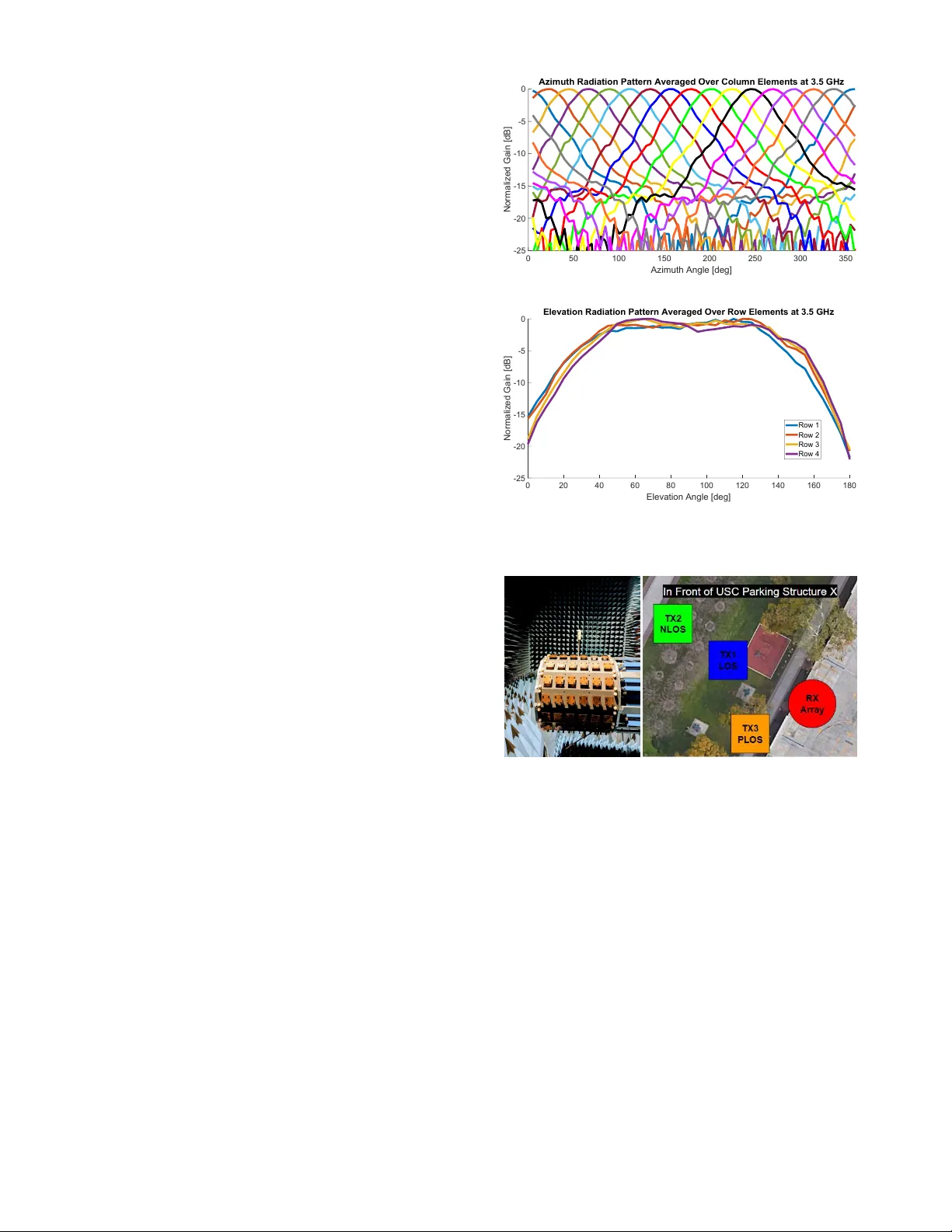
Channel Extrapolation for FDD Massi v e MIMO: Procedure and Experimental Results Thomas Choi ∗ , François Rottenberg ∗ , Jorge Gomez-Ponce ∗ , Akshay Ramesh ∗ , Peng Luo ∗ Jianzhong Zhang † , and Andreas F . Molisch ∗ ∗ Univ ersity of Southern California, Los Angeles, CA, USA † Samsung Research America, Richardson, TX, USA Abstract —Application of massive multiple-input multiple- output (MIMO) systems to frequency division duplex (FDD) is challenging mainly due to the considerable overhead r equired for downlink training and feedback. Channel extrapolation, i.e. , estimating the channel response at the downlink frequency band based on measurements in the disjoint uplink band, is a pr omising solution to over come this bottleneck. This paper presents measurement campaigns obtained by using a wideband (350 MHz) channel sounder at 3.5 GHz composed of a cali- brated 64 element antenna array , in both an anechoic chamber and outdoor en vironment. The Space Alternating Generalized Expectation-Maximization (SA GE) algorithm was used to extract the parameters (amplitude, delay , and angular information) of the multipath components fr om the attained channel data within the “training” (uplink) band. The channel in the downlink band is then reconstructed based on these path parameters. The performance of the extrapolated channel is evaluated in terms of mean squared error (MSE) and reduction of beamforming gain (RBG) in comparison to the “ground truth”, i.e. , the measured channel at th e downlink fr equency . W e find str ong sensitivity to calibration errors and model mismatch, and also find that performance depends on propagation conditions: LOS performs significantly better than NLOS. I . I N T RO D U C T I O N Massiv e multiple-input multiple-output (MIMO) will be an essential part of 5G and beyond wireless communications sys- tems. While massiv e MIMO performs generally better using time division duplex (TDD) than frequency division duplex (FDD) [1], frequency regulators ov er the world hav e assigned large swathes of v aluable spectrum as band pairs for FDD operation; furthermore backward compatibility considerations ( e.g . , with Long-T erm Ev olution (L TE)) also often require FDD operation. Enabling FDD massi ve MIMO has thus been a popular research topic in recent years [2]–[4]. The key challenge lies in the acquisition of channel state information for the downlink. Current systems use downlink training and feedback from the user equipment (UE) to the base station (BS), which leads to considerable ov erhead. An alternative is frequency extrapolation, i.e. , using channel information measured in the uplink frequency band to estimate channel information in the do wnlink frequency band. The idea of frequency extrapolation for MIMO systems has been studied in the past. One avenue of research was the e xtrapolation of second-order channel c haracteristics such as angular power spectra and correlation matrices. It can be argued from physical considerations that the directions from which the dominant powers are coming change only weakly with frequency . Angular power spectra deriv ed from Bartlett and Capon beamformers were used in [5] for 4 × 4 MIMO. The authors in [6] performed frequency extrapolation of ex- tracted dominant angles using maximum-likelihood directional estimators for 64-element arrays and combined them with an ingenious training/feedback scheme. Another , more difficult, goal is the extrapolation of the complex, instantaneous channel frequency response. Since the phases of the multipath components (MPCs) change rapidly ov er frequency , such an extrapolation is extremely sensitive to both measurement errors within the training band, and errors in the extrapolation algorithm. While theoretical in vestigations and e xperiments based on synthetic channel models have been performed for a while [7]–[10], ev aluations based on indoor and outdoor measurements hav e been done only recently . In particular , extrapolation based on a Fourier representation of the channel using uniform linear arrays for 4 to 16 antenna elements w as done in [11]. Deep learning based frequency extrapolation with 32 antenna elements showed sum-rates information for measured MIMO cases in [12]. In all these cases, the “training bandwidth” ( i.e . , the bandwidth in which the channel was measured for estimation), was between 10 to 20 MHz, while the extrapolation range was between 40 to 72 MHz. Most of these in vestigations present the results in terms of achiev able beamforming gain, SNR, or data rate. In this paper , we present results from a measurement campaign in both an anechoic chamber and a realistic outdoor scenarios. Results indicate error sources such as calibration errors lead to worse performance than theoretical bounds [10], [13]. As our in vestigation in [10], our e xtrapolation approach is based on (i) measuring with a calibrated array , (ii) extracting the MPC parameters with a high resolution parameter esti- mation (HRPE) algorithm (the Space Alternating Generalized Expectation-Maximization (SAGE) algorithm [14]), and (iii) synthesizing the channel response at the ne w band. Our measurements have the follo wing characteristics. First, channel measurements are done with a wideband (350 MHz), real-time time-domain channel sounder that allows to mimic operation of a 5G system. Second, we perform our measure- ments in an outdoor en vironment under a variety of setups, including line-of-sight (LOS), non-LOS (NLOS), and partial LOS (PLOS), encountering real channel conditions that might deviate from the model (finite sum of plane wav es) that forms the basis of the extrapolation. Third, calibration and measure- ments are done with different mountings (rotating positioner and measurement cart respecti vely), with some time between them, providing information about sensitivity to calibration “aging” and its impact on the extrapolation. Last b ut not least, we in vestigate dif ferent metrics to judge the quality of the extrapolation, especially comparing mean squared error (MSE) and reduction of beamforming gain (RBG). The paper is organized as follo ws. Section II describes channel sounder specifications, antenna array calibration, and measurement scenarios. Section III describes the process of applying SAGE to the measured data and extrapolating the channel. Measurement results in Section IV quantify the result- ing MSE and RBG of estimated channels in the extrapolated frequency bands, follo wed by their implications for practical channel extrapolation in the frequency domain. Section V provides the conclusions and indications of our future work. I I . S O U N D E R , C A L I B R AT I O N , A N D M E A S U R E M E N T A. Channel Sounder Specifications Massiv e MIMO usually refers to a BS with a large number of antenna elements communicating with a multitude of single- antenna UEs. Since the channel estimation errors for the different UEs are independent of each other provided that they use orthogonal training sequences, it is sufficient to analyze a single-input multiple-output (SIMO) setup; such a setup was used for our real-time channel sounder . Figure 1 and T able 1 show the photo and the specifications of the Univ ersity of Southern California (USC) SIMO channel sounder . W e chose the 3.5 GHz frequency band for the sounder because it will be used widely for 5G and beyond. USC obtained an experimental license to operate at the frequenc y from the Federal Communications Commission (FCC). On the transmitter (TX) side, the sounder uses a single omni-directional antenna. The antenna has a non-uniform beampattern in elev ation, with a beamwidth (full-width half- maximum, FWHM) of ∼ 90 °. Note that due to the SIMO setup, extraction of angles of departure is not possible, which may be one of the error sources in the extraction of the MPC parameters [15] when the antenna characteristics are not separable in angle and frequency; the campaign in this paper kept the error small by measuring in outdoor scenarios with limited elev ation spread. The receiver (RX) uses a cylindrical 64 element array . Patch antenna elements are put together in 16 columns, where each column contains 4 active patches in the middle (forming 4 rows), plus a dummy patch (terminated with 50 ohm loads) each at the top and bottom. Each element has one vertically polarized and one horizontally polarized port. While the measurements were conducted with all 128 ports, only 64 vertically polarized ports were used for ev aluation of the channel. The reason is because cross-polarized ports in RX had failed to provide consistent radiation patterns during calibration due to high noise sensitivity (TX is vertically polarized). Note that the lack of dual-polarization at TX and RX might also contribute to modeling errors [15]. Each vertically polarized port has azimuth beamwidth of 50 ° and elev ation beamwidth of 100 ° (see Fig. 2). The “stacked” patch design provides a wide bandwidth ( S 11 < − 10 dB), ∼ 10% of the center frequency ( ∼ 350 MHz of 3.5 GHz). The sounder operates according to the switched sounding principle, where a single Radio Frequency (RF) chain is sequentially connected to each of the 128 ports by a fast (100 ns switching time) electronic switch. The noise figure of the RX RF chain varies, with up to 11 dB when the variable attenuator (required for adjustments to large input lev el v ariations) in the chain is at 30 dB, and do wn to 2.5 dB when v ariable attenuator is at 0 dB. At the TX, an arbitrary wa veform generator (A WG) creates a 350 MHz bandwidth multitone signal containing 2801 sub- carriers (frequency spacing of 0 . 125 MHz). Using waveform from [16], the lo w peak-to-average po wer ratio (P APR) of 0 . 4 dB allows the system to transmit with power close to the 1 dB compression point of the power amplifier without saturation; the emitted equiv alent isotropically radiated power (EIRP) is 30 dBm. Each wav eform lasts 8 µ s. This wav eform is repeated 10 times to increase the signal to noise ratio (SNR) by av eraging, increasing the duration of one SISO measurement ( i.e. , between the TX antenna and one RX port) to 80 µ s. The total SIMO sounding duration is 128 × 0 . 08 = 10 . 24 ms. Hardware Specs Center frequency 3.5 GHz # of TX/RX ports 1/64 TX EIRP 30 dBm RX beamwidth az/el 50°/100° RX RF switch time 100 ns RX total noise figure < 11 dB Sounding W aveform Bandwidth 350 MHz Sample frequency 1.25GSps # of subcarriers 2801 P APR 0.4 dB W aveform duration 8 us W aveform repetition 10 SISO duration 80 us SIMO duration 10.24 ms Fig. 1 & T ABLE I: USC SIMO channel sounder B. Calibration of Antennas and RF Chains The wav eform measured at the analog to digital conv erter (ADC) at the RX contains the transmitted w av eform affected by antennas, RF chains, and the channel. Therefore, calibra- tions of the antennas and the RF chains are necessary in order obtain the true physical characteristics (amplitude, delay , and angular information) of the channel itself. This subsection discusses the calibration procedures; usage of the calibrated data for HRPE will be discussed in Sec. III. The TX antenna and the RX array (including the switches) are calibrated “together”. T wo ports on the vector network analyzer (VN A) are connected to the input port of the TX antenna and output port of the switch at RX. This setup is placed in the shielded anechoic chamber at USC. TX and RX were placed at least 5 m from each other, which is larger than the Rayleigh distance of the array at the highest considered frequency ( 2 D 2 /λ = 3 m), so that the far-field assumption holds. While TX antenna is fixed in one position, the RX array is on a rotating positioner that moves the array in 5 ° steps in both azimuth ( 360 °) and elev ation ( 180 °), providing 72 × 37 positions. The positioner was covered with absorbers to minimize its impact on the measured array patterns. For each position, the array switches through the 128 ports, and for each switch position, the VN A sweeps to get frequenc y response per port per position. During the calibration, the TX power was 10 dBm, and a low-noise amplifier (whose impact on the frequency characteristics was eliminated in post- processing) was placed in front of the VN A receiving port, in order to increase the SNR during calibration to 50 dB. The calibration provides a 4-Dimensional calibration matrix ( por t × az imuth × el evation × f r equency ) characterizing the antennas. This complex pattern a ( m, φ, θ , f ) , compensated by free space path loss, serves as a reference radiation pattern that is an input for the SA GE algorithm. Fig. 2 shows the av eraged azimuth pattern and ele vation pattern ov er column and row respectiv ely at 3.5 GHz. Because frequency points measured during the calibration are fewer than the frequency points used in channel sounder (every 1 MHz vs e very 0.125 MHz), the ef fectiv e aperture distribution function (EADF) was used to interpolate the pattern in ele vation and azimuth angles on unmeasured frequenc y points. [17]. Calibrating RF chain to obtain the so-called “RF back-to- back” frequency response, H b 2 b , is rather simple. The TX output (at the TX antenna connector) is connected directly (via a cable) to the RX input (at the point where normally the switch output would be connected), with attenuators in between to prev ent the high power output from the TX saturating the RF components in the RX. Frequenc y responses of the attenuators and cables are then measured separately , and compensated from the frequency response of the back-to-back measurements that include them. H b 2 b ( f ) is one-dimensional complex valued vector , depending only on frequenc y . C. Measur ement Scenarios For initial verification of the setup functionality , first mea- surements were conducted in the anechoic chamber right after the calibration. TX antenna and RX array remained in the same position as during calibration (RX array still attached to the positioner), as shown in Fig. 3 to minimize calibration error . Then, outdoor measurements were conducted, where a TX antenna was 1 m above ground at three dif ferent positions and the RX array was on top of a four stories high parking structure (USC PSX building) sitting on top of a cart. The three different positions for TX covered scenarios which were LOS, PLOS (where only parts of the arrays were at LOS due to a waist-high wall - example: only 1st row of all 4 rows was at LOS), and NLOS, where the LOS connection was blocked by trees. Lastly , the sounder was mov ed back onto 0 50 100 150 200 250 300 350 Azimuth Angle [deg] -25 -20 -15 -10 -5 0 Normalized Gain [dB] Azimuth Radiation Pattern Averaged Over Column Elements at 3.5 GHz (a) Azimuth 0 20 40 60 80 100 120 140 160 180 Elevation Angle [deg] -25 -20 -15 -10 -5 0 Normalized Gain [dB] Elevation Radiation Pattern Averaged Over Row Elements at 3.5 GHz Row 1 Row 2 Row 3 Row 4 (b) Elev ation Fig. 2: Calibrated radiation patterns for a 64 V -pol ports (a) Chamber (b) Outdoor Fig. 3: T wo dif ferent measurement scenarios the positioner , and another LOS measurement was done in the anechoic chamber . As the outdoor measurement studies were conducted two months after the calibration, the objective of this third experiment was to verify whether calibration has been retained, to narrow do wn potential error sources in our studies. I I I . F R E Q U E N C Y E X T R A P O L A T I O N This section re views the principle of HRPE-based channel extrapolation and defines the figures of merit of this study , MSE and RBG, from measurement data and calibration data. In brief, we extract from measurements within a “training bandwidth” the MPC parameters through HRPE, and use them to synthesize the transfer function in the desired frequency band; the figures of merit describe the difference between these extrapolated transfer functions and the ground truth, i.e. , the actually measured transfer function in the desired band. Figure 4 outlines the detailed steps. While the calibration data obtained with the VNA provides the frequency re- sponse directly , the (time-domain) measurement data recei ved from the ADC are Fourier -transformed (after cyclic prefix remov al) to provide the frequency response. It is av eraged ov er the wa veform repetitions to impro ve the SNR, providing H meas ( m, f ) where m is the port number and f is frequenc y in Hz (there are in total 64 ports and 2801 frequency points, as specified in T ABLE 1). The frequenc y response of the RF chain obtained through RF back-to-back calibration (see Sec- tion II-B), H b 2 b ( f ) , is remov ed from H meas ( m, f ) to provide H chan ( m, f ) , which is a combined response of channel, TX antenna, and RX array . In order to analyze channel extrapolation, a “training band- width”, i.e. , a subset of total measurement bandwidth, is se- lected (in a practical system this would be the bandwidth ov er which the BS can observe uplink pilots). Among all measured frequency points, those within this training bandwidth are referred as f tb . In this particular study , the first 35 MHz (3.325 - 3.360 GHz) of 350 MHz bandwidth was chosen, which corresponded to 281 of 2801 frequency points. The subset of H chan ( m, f ) , denoted as H chan ( m, f tb ) , and the calibrated complex pattern of TX antenna and RX array , a ( m, φ, θ , f ) (see Section II-B), are used as inputs for SAGE algorithm, a widely popular HRPE algorithm [14]. The SA GE algorithm models the transfer functions at the different antenna elements as the sum of plane wav es (MPCs): H S AGE ( m, f ) ∆ = L X l =1 ˆ α l a ( m, ˆ φ, ˆ θ , f ) e − 2 π jf ˆ τ l . (1) This model has a number of important implicit assumptions: e.g . , that the absolute amplitude of an MPC is constant across the different antenna elements, and that no wa ve- front curvature exists. A further important question is the number of modeled paths L . A larger L might be required to represent a sufficient percentage of the total field; yet increasing the number of estimated parameters might also increase the estimation errors due to ov er-fitting. Thus, while L ≤ 4 might be suf ficient for extrapolation if the scenario is very simple (example: LOS scenario in anechoic chamber), complicated scenarios may require as much as > 20 paths. Finally , we note that SA GE is an iterative algorithm that might con verge to a local minimum, depending on initialization and various iteration parameters; for more details see, e .g. , [14]. The output from SAGE are the parameters of the MPCs, which include complex amplitude, delay , azimuth and elev a- tion ( ψ l − S AGE = [ ˆ α l , ˆ τ l , ˆ φ l , ˆ θ l ]). From these parameters, the SIMO channel model is used to reconstruct the channel for each port at each frequency using equation (1). Note that this approach provides the extrapolated channel in the uplink . T o be used in an actual system, the channel and associated beamformer needs to be translated to the equiv alent downlink channel. Our measurement setup is not designed R e d u c ti on i n Be amfor mi n g G ai n F re que nc y re s pons e of c ha nne l , T X a nt e nna , a nd R X a rra y F re que nc y re s pons e of c ha nne l , T X a nt e nna , a nd RX a rra y for “ tr ai n i n g b an d w i d th ” Ca l i bra t e d F re que nc y re s pons e of T X a nt e nna a nd RX a rra y S A G E a l gori t hm F re que nc y re s pons e of m e a s ur e m e nt Mea s u reme n t Cal i b ra t i o n F re que nc y re s pons e of RF s ys t e m (Ba c k - to - Ba c k) # of pa t hs t o e s t i m a t e P a t h pa ra m e t e rs from S A G E S A G E c ha nne l m ode l M e an S q u ar e d Er r or     󰇛  󰇜     󰇛    󰇜              󰇛    󰇜     󰇛  󰇜   󰇛        󰇜                   󰇟                󰇠                󰇛            󰇜              󰇛  󰇜                  󰇛    󰇜           󰇛  󰇜   󰇛              󰇜      󰇛             󰇜                                   Fig. 4: Process of frequency extrapolation to include this step, which is also known as reciprocity calibration. Ho wever , it is the same as in TDD systems, where it has been widely explored [18]. Furthermore, any errors occurring in this step would be additive to, and essentially independent of, the errors from the extrapolation procedure. Lastly , both H chan ( m, f ) and H S AGE ( m, f ) are used to calculate both the MSE and the RBG for the extrapolated channel at any frequenc y f of interest. First, MSE is calculated as follow: M S E ( f ) ∆ = P M m =1 | H chan ( m, f ) − H S AGE ( m, f ) | 2 M (2) where M is the number of ports ev aluated (in our case, M = 64 ). If f lies within the training bandwidth, the MSE describes the classical accurac y of the SA GE-extracted MPCs for channel sounding; for f outside the training band, it describes the quality of the channel extrapolation. Also, the RBG refers to how much loss occurs with knowl- edge of estimated channel response assuming matched filter . Knowledge of H S AGE is compared to the perfect channel knowledge, which in our study refers to kno wledge of H chan (min RBG = 1 = 0 dB). RB G ( f ) ∆ = ( P M m 0 =1 | H S AGE ( m 0 , f ) | 2 )( P M m 00 | H chan ( m 00 , f ) | 2 ) | P M m 000 =1 H ∗ S AGE ( m 000 , f ) H chan ( m 000 , f ) | 2 (3) I V . R E S U LT S A N D D I S C U S S I O N S Fig. 5 and Fig. 6 show results of MSE and RBG in the outdoor and chamber environments (Fig. 3). W e see that outside the training bandwidth, the MSE is usually lar ger than − 10 dB, and often approaches or e ven e xceeds 0 dB for NLOS case. W e discuss in the follo wing some main insights on the channel properties the error depends on. First, we consider the error within the training bandwidth ( 3 . 325 − 3 . 36 GHz), henceforth called reconstruction err or . Its value depends on the particular scenario: for the LOS cases, MSE was < − 15 dB, but increases as the channel mo ves from LOS, to NLOS. This may be due both to a reduction of the SNR, and the fact that a richer multipath en vironment makes the estimation of the MPC parameters more difficult due to interpath interference. W e also see that the reconstruction error is e ven lar ger in the PLOS channel, where some rows are at LOS and other rows are at NLOS. This can be explained by the fact that PLOS violates the fundamental SAGE signal model, as the absolute amplitude of the MPCs across the antenna elements is not constant. The MSE outside the training bandwidth (henceforth called extr apolation err or ) remains, for the LOS case, < − 10 dB for up to 70 MHz distance from the 35 MHz training band. Furthermore, the extrapolation error in terms of MSE increases as the channel mov es from LOS, to NLOS, to PLOS for up to 40 MHz distance from the training band. W e also find that for all scenarios an increase in the number of estimated paths L leads to a lo wer reconstruction error - it is intuitiv e that a more sophisticated model can better represent the channel within the measured bandwidth; it can e ven correct partially for model mismatch, e.g., by approximating a curved wa vefront by a sum of plane wav es. This situation changes when we consider the extrapolation error . There, the MSE becomes worse as we increase L from 4 to 20. This is due to the fact that estimation errors in the delay are more pronounced for the additional, weaker (lower SNR) MPCs that are estimated in the latter case; delay estimation errors strongly impact the phase at extrapolated frequencies. The increase of the extrapolation error with increasing L is most pronounced in the LOS case, mostly because for NLOS the error is high ov erall anyway . Besides the MSE, we are also interested in the loss of beamforming gain. Fig. 5b shows the results for the different en vironments. W e see that for the LOS scenario, the loss is less than 1.2 dB over the whole 350 MHz bandwidth, while for NLOS, the loss in less than 2 dB until 165 MHz outside the band (3.325 - 3.525 GHz). It is worth remembering that the ideal beamforming g ain achieved in our system is 18 dB, so even a 3 dB loss is comparatively lo w . Still, the relativ ely high extrapolation error motiv ated us to in vestigate possible error sources. The key candidates were (i) model mismatch, and (ii) calibration errors. In terms of model mismatch, we already noted that the PLOS setup results in a violation of the model assumption of absolute amplitude of the MPCs across the antenna elements being constant, so 3.35 3.4 3.45 3.5 3.55 3.6 3.65 Frequency [Hz] 10 9 -20 -15 -10 -5 0 5 MSE [dB] MSE - Outdoor Measurement (06-03-19) LOS: 4 Paths NLOS: 4 Paths P-LOS: 4 Paths LOS: 20 Paths NLOS: 20 Paths PLOS: 20 Paths Training BW 3.325 - 3.36 GHz (a) MSE - outdoors 3.35 3.4 3.45 3.5 3.55 3.6 3.65 Frequency [Hz] 10 9 12 10 8 6 4 2 0 Reduction in Beamforming Gain [dB] RBG - Outdoor Measurement (06-03-19) LOS: 4 Paths NLOS: 4 paths PLOS: 4 paths LOS: 20 paths NLOS: 20 paths PLOS: 20 paths Training BW 3.325 - 3.36 GHz (b) Reduction in beamforming gain - outdoors Fig. 5: Results from outdoor measurements 3.35 3.4 3.45 3.5 3.55 3.6 3.65 Frequency [Hz] 10 9 -20 -15 -10 -5 0 MSE [dB] MSE - Chamber Measurement 04-04-19 06-07-19 Training BW 3.325 - 3.36 GHz (a) MSE - chamber 3.35 3.4 3.45 3.5 3.55 3.6 3.65 Frequency [Hz] 10 9 0.4 0.3 0.2 0.1 0 Reduction in Beamforming Gain [dB] RBG - Chamber Measurement 04-04-19 06-07-19 Training BW 3.325 - 3.36 GHz (b) Reduction of beamforming gain - chamber Fig. 6: Results from chamber measurements (LOS) that both reconstruction error and extrapolation error are high. Howe ver , this does not completely explain the extrapolation error for NLOS, since the reconstruction error for this scenario is smaller than in PLOS, but extrapolation error is much larger . T o test the calibration error , we had performed simple LOS measurements in the anechoic chamber, see Fig. 6. W e see that in the measurements conducted right after the calibration (see black line, denoted by 04-04), the extrapolation error is small - less than − 10 dB up to 200 MHz distance from the training band. Howe ver , for a measurement that was conducted after two months since the calibration (see purple plots, 06-07), performance degraded considerably (note that while the measurement was conducted in the same chamber, the measurements are not exactly comparable due to modified setups within the chamber , as indicated also by the fact that the reconstruction error of the later measurements is actually smaller than that of the earlier measurements). Furthermore, the MPC parameters extracted from the chamber measure- ments agree with the physical conditions, i.e . , directions and delay of the MPC components. RBG was actually less for (06- 07) in comparison to (04-04), despite worse performance in MSE, (in all cases the actual RBG is small anyways due to very simple and optimistic scenario). This indicates that calibration has been lost to a certain de- gree in those two months, despite the fact that the array/switch combination was not altered consciously . W e cannot exclude the possibility that aging of the material of the patches (copper oxidization), small mov ement of cables due to vibrations during transport, and other irreproducible effects lead to the change in calibration. W e stress that while such miniscule calibration change strongly affected the channel extrapolation error , it did not affect the HRPE parameters, so that it would not be noticed in a regular high-resolution channel sounding campaign. V . C O N C L U S I O N W e hav e provided e xperimental results for frequency e xtrap- olation of the channel transfer function based on HRPE. Our experiments resulted in an MSE that in most outdoor cases was above − 10 dB outside 35 Mhz training band, implying that the extrapolation of the instantaneous channel response is highly sensitiv e to calibration errors. On the other hand, in terms of beamforming gain, the results looked more promising. This implies that a large MSE does not necessarily induce a high loss in beamforming power . In conclusion, our results do not necessarily imply that the channel extrapolation for FDD massiv e MIMO cannot be used in practice. Other papers [6], [11], [12] showed its possibilities using other figures of merit and methods. For our future works, we will study other figures of merit to e valuate the performance of channel extrapolation using v arious HRPE algorithms. Also, the methods to keep calibration as consistent as possible will be studied. Lastly , the measurements will be extended to full MIMO system to see effects of number of antennas on both TX and RX ends. Acknowledgement: Part of this work was supported by NSF EECS-1731694, a gift from Samsung America, and the Bel- gian American Educational Foundation (B.A.E.F .). Measure- ment help from Zihang Cheng is gratefully acknowledged. R E F E R E N C E S [1] J. Flordelis, F . Rusek, F . Tufv esson, E. G. Larsson, and O. Edfors, “Mas- siv e MIMO Performance—TDD V ersus FDD: What Do Measurements Say?” IEEE T ransactions on Wir eless Communications , vol. 17, no. 4, pp. 2247–2261, April 2018. [2] Y . Nam, B. L. Ng, K. Sayana, Y . Li, J. Zhang, Y . Kim, and J. Lee, “Full- dimension MIMO (FD-MIMO) for next generation cellular technology, ” IEEE Communications Magazine , vol. 51, no. 6, pp. 172–179, June 2013. [3] J. Choi, D. J. Love, and P . Bidigare, “Downlink Training T echniques for FDD Massive MIMO Systems: Open-Loop and Closed-Loop Training W ith Memory, ” IEEE J ournal of Selected T opics in Signal Pr ocessing , vol. 8, no. 5, pp. 802–814, Oct 2014. [4] Z. Jiang, A. F . Molisch, G. Caire, and Z. Niu, “Achiev able Rates of FDD Massive MIMO Systems With Spatial Channel Correlation, ” IEEE T ransactions on Wir eless Communications , v ol. 14, no. 5, pp. 2868– 2882, May 2015. [5] M. Matthaiou, N. Razavi-Ghods, D. I. Laurenson, and S. Salous, “Dual frequency MIMO measurements in the 2.26-2.5 GHz band, ” W ir eless Communications and Mobile Computing , v ol. 8, no. 5, pp. 607–614, Nov 2008. [Online]. A vailable: https://doi.or g/10.1002/wcm.573 [6] X. Zhang, L. Zhong, and A. Sabharwal, “Directional Training for FDD Massiv e MIMO, ” IEEE T ransactions on W ireless Communications , vol. 17, no. 8, pp. 5183–5197, Aug 2018. [7] M. Pun, A. F . Molisch, P . Orlik, and A. Okazaki, “Super -Resolution Blind Channel Modeling, ” in 2011 IEEE International Confer ence on Communications (ICC) , June 2011, pp. 1–5. [8] U. Ugurlu, R. Wichman, C. B. Ribeiro, and C. Wijting, “A Multipath Extraction-Based CSI Acquisition Method for FDD Cellular Networks W ith Massiv e Antenna Arrays, ” IEEE T ransactions on W ireless Com- munications , v ol. 15, no. 4, pp. 2940–2953, April 2016. [9] W . Y ang, L. Chen, and Y . E. Liu, “Super-Resolution for Achieving Frequency Division Duplex (FDD) Channel Reciprocity , ” in 2018 IEEE 19th International W orkshop on Signal Pr ocessing Advances in W ireless Communications (SP A WC) , June 2018, pp. 1–5. [10] F . Rottenberg, R. W ang, J. Zhang, and A. F . Molisch, “Channel Extrap- olation in FDD Massiv e MIMO: Theoretical Analysis and Numerical V alidation, ” arXiv preprint:1902.06844 , Feb 2019. [11] D. V asisht, S. Kumar , H. Rahul, and D. Katabi, “Eliminating Channel Feedback in Next-Generation Cellular Networks, ” in Pr oceedings of the 2016 ACM SIGCOMM Confer ence , ser. SIGCOMM ’16. New Y ork, NY , USA: A CM, 2016, pp. 398–411. [12] M. Arnold, S. Dörner, S. Cammerer, S. Y an, J. Hoydis, and S. ten Brink, “Enabling FDD Massive MIMO through Deep Learning-based Channel Prediction, ” arXiv e-prints , p. arXi v:1901.03664, Jan 2019. [13] M. D. Larsen, A. L. Swindlehurst, and T . Svantesson, “Performance Bounds for MIMO-OFDM Channel Estimation, ” IEEE T ransactions on Signal Pr ocessing , vol. 57, no. 5, pp. 1901–1916, May 2009. [14] B. H. Fleury, M. Tschudin, R. Heddergott, D. Dahlhaus, and K. Ingeman Pedersen, “Channel Parameter Estimation in Mobile Radio Environ- ments Using the SAGE Algorithm, ” IEEE J. Sel. Areas Commun. , vol. 17, no. 3, pp. 434–450, March 1999. [15] M. Landmann, M. Kaske, and R. S. Thoma, “Impact of Incomplete and Inaccurate Data Models on High Resolution Parameter Estimation in Multidimensional Channel Sounding, ” IEEE T ransactions on Antennas and Pr opagation , v ol. 60, no. 2, pp. 557–573, Feb 2012. [16] M. Friese, “Multitone Signals with Low Crest Factor , ” IEEE T ransac- tions on Communications , vol. 45, no. 10, pp. 1338–1344, Oct 1997. [17] A. Richter , “Estimation of radio channel parameters: Models and al- gorithms, ” Ph.D. dissertation, Elektronische Messtechnik at T echnische Univ ersität Ilmenau, Ilmenau, Germany , 2005. [18] J. V ieira, F . Rusek, O. Edfors, S. Malkowsky, L. Liu, and F . T ufvesson, “Reciprocity Calibration for Massiv e MIMO: Proposal, Modeling, and V alidation, ” IEEE Tr ansactions on Wir eless Communications , v ol. 16, no. 5, pp. 3042–3056, May 2017.