Data augmentation in microscopic images for material data mining

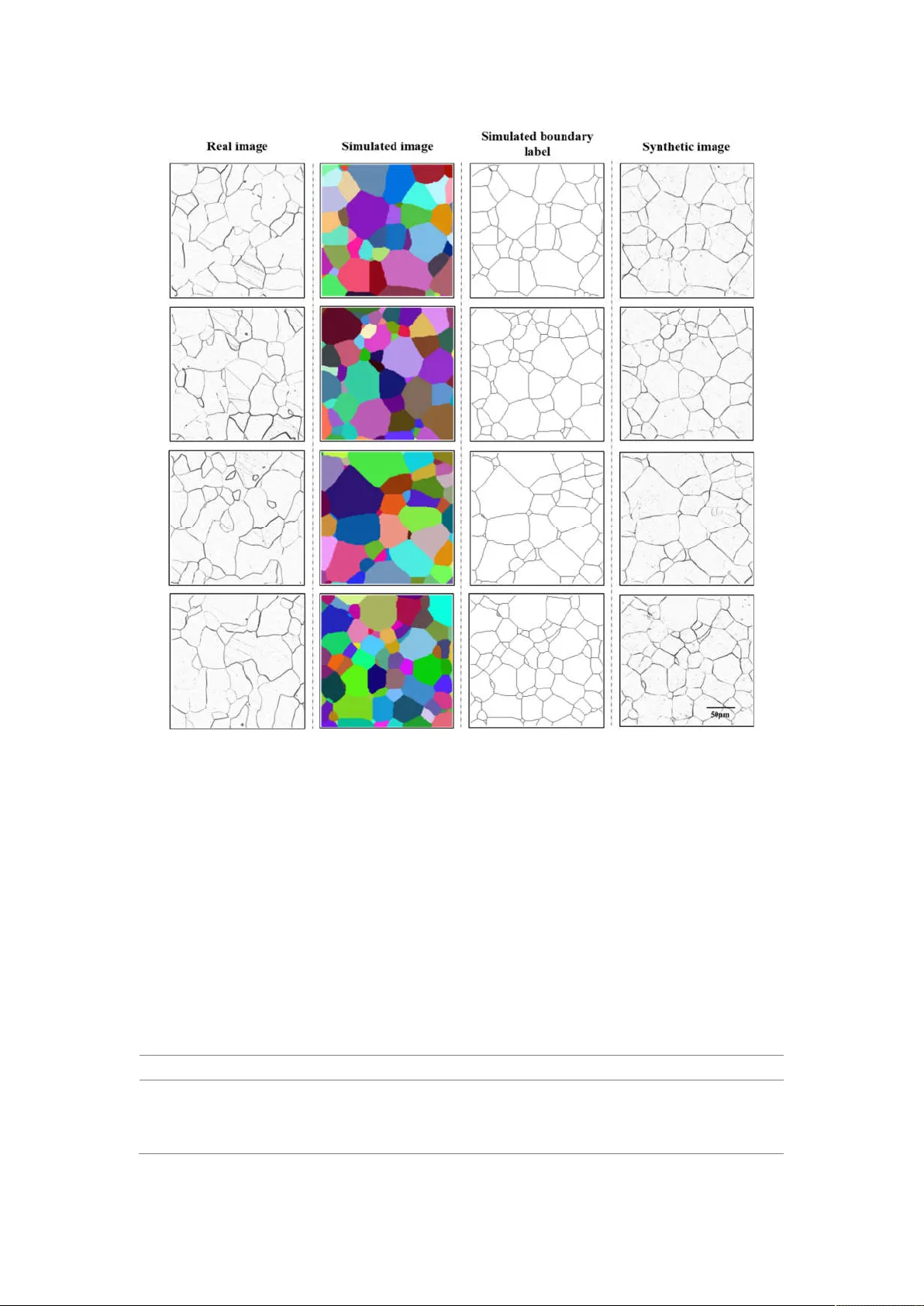
Data augm entation in m icroscopic images for material data m ining Boyuan Ma a, b, c , Xiaoyan W ei a, b, c , Chuni Liu a, b, c , Xiaojuan Ban a, b, c,* , Haiyou Huang a, c, d, ** , Hao W ang a, e , W eihua Xue e, f , Stephen W u g,*** , Mingfei Gao a, b, c , Qing Shen h , A dnan Omer Abuassba i , Haokai Shen j, k , Y anjing Su a, l a. Beijing Advanced Innovation Center for Materials Ge nome Engineeri ng, University of Sci ence and T echnology Beijing, Beij ing, 100083, China. b. School of Com puter and Communication Engineering, University of Science and T echnolog y Beijing, Beij ing, 100083, China. c. Beijing Key Labo ratory of Kno wledge Engineering for Mate rials Science, B eijing, 100 083, China. d. Institute for Advanced Materials and T echnology , Universit y of Science and T echnology B eijing, Beijing, 100 083, China. e. School of Materia ls Science and Engineering, University of Science and T echnology Beijing, Beijing, 100 083, China. f. School of Materials Scie nce and T echnology , Liaoning T echnical University , Liaoning, 114051, China. g. The Institute of Statistical Mathematics, Research Organization of Information and Systems, T achikawa, T oky o 190-85 62, Japan. h. National intellectual pr operty administratio n, Beijing, 100 088, China. i. Arab Open Univer sity , Palestine, Ra mallah, Palestine. j. College of Infor mation Science and E ngineering, China U niversity of Petro leum, Beijing, China. k. Key Lab of P etroleum Data Mining, China University of P etroleum, Beij ing, China. l. Corrosion and Protection Center , University of Science a nd T echnology Beijing, Beijing, 100083, China. * Corresponding author at: School of Computer and Communicat ion Engineering, University of Science and T echnology Beijing, Xuey uan Road 30, Haidian Dist rict, Beijing 1000 83, China. Email addresses: banxj@ustb.edu.cn. ** Corresponding author at: Institute for Advanced Materi als and T echnology , University of Science and T echnology Beijing, Xueyuan Road 30, Haidian District, Beijing 100083, China . Email a ddresses: huanghy @mater .ustb.edu.cn. *** Corresponding author at: Research Organi zation of Informat ion and Systems, The Inst itute of Statisti cal Mathem atics, T achikawa, T okyo 190- 8562, Japan; Email addresses: stewu@ism.ac. jp . Abstract Recent progress in material data mini ng has been driven by high-capaci ty model s trained on large datasets. However , collecting experim ental data (real data) has been extremely costly since the amount of human ef fort and expert ise required . Here, we dev elop a novel transfer l earning s trategy to addres s sm all or insuf ficient data problem . This strategy real izes the fusion of real and sim ulated data, and the augm entation of training data in data mini n g procedure. For a specific t ask of image segment ation, this s trategy can generate synthetic images by fusing physical mechanism of sim ulated i mages and “image style” of real i mages. The result shows that the m odel trained with the acquired syntheti c i mages and 35% of the real images outperform s the model trained on all real image s. As the time required to generate synthe tic data is almost negligible, this strategy is able to reduce the tim e cost of real data preparat ion by roughly 65%. Introduction There has been considerabl e interest over the last few years in accelerating the process of materials design and discovery [1]. In the past decade, accelerating discovery relied o n databases, computati on, m athe mat ics and information science has created more and more succe ssful cases in the materi a ls sciences [2-6]. In general, the larger the training dataset is, the more accurate the machine learni ng model becomes. Especial ly for deep neural networks, whic h have shown to have exceptional prediction performance when trained with a large amount of data. As a result, some accelerate methods for data accumulati on, such as high-throughput computation and high- throughput experi ment, hav e been developed to build lar ge databases. However , in many m aterials researches, especially for new materials, we still have to face the dilemma of lacking high- quality data due to a tim e-consum ing or technically diffi cult process of collecting experiment al data (real data) and a low ac curacy of com putational data. Material m icrostructure data is an important ty pe of material dat a to build the intrinsic relationship of com position, structure, process and properties, which is fundamental to materi al design. Therefore, the quantitativ e analysis of microstructures is essential for the control of the properties and performances of metal s or alloys [7-8]. One of the most important steps in this process is microscopi c image processing using comput ational algorithm s and tools [9-10]. For example , image segmentation [1 1], which outputs the pixel-wise label of original image, is commonly used to extract significant information in microscopic images at the field of materi al structure characterizat ion [12]. T ake polycryst alline iron for example , as shown in Figure 1(a) and (b), which is a basic and typical case in practical material research, the objective of image processi ng algorithm is to detect grain boundary fro m raw microscopic image in order to obtai n accurate micros tructure infor mation, such as geom etric and t opological chara cterist ics. Figure 1. Microscopic images of polycrystalline iron. (a) Raw real experimental image obtained by optical microscope. (b) Grain boundary detection result of (a) conducted by human, it was used as ground truth in our investigation. (c) A 3D simulated m od el. (d) One slice of image from the 3D model, the so-called simulated image. (e) Boundary detection label of (d). Recent progress in m aterial m icroscopic image segmentation [13-15] has been driven by high - capacity models trai ned on lar ge datasets. Unfortunately , the generalization performance of these models is hindered by the lack of la r ge dataset due to tim e-consuming labeling of m aterial micros copic images. Creating lar ge datasets with pixel- wise semant ic labels is known to be very challenging due to the amount of human effort and expertise required to trace ac curate object boundaries [16]. Therefore, such lar ge datasets with pixel-wise label for image segment ation are often hard to o btain. In this work, we develop a nov el tr ansfer learning strateg y to address smal l or insuffi cient data problem in material data mining. This strategy r ealizes the fusion of real data and sim ulated/calculat ed data based on transfer learning theory , and the aug ment ation of trai ning data in data m ining procedur e, so that classi fication or regression m odel with better per form ance can be established based o n only a sm all set of real data. W e explore the use of 3D si mulated model to create large- scale pixel- accurate data fo r training image segmentation systems. F or exa mple, as show n in F igure 1(c) , a Mont e Carlo P ott s model can represent poly crystalline microstruct ure of materials, which turns out to possess similar geometri cally and topological ly microstructure characterist ics of grains compared to the real grain structure [17- 18]. It is easy to get large slice (image) data with pixel-lev el label from sim ulated 3D model using computational methods , see Figure 1 (d) and (e). However , acquired contents in sim ulated im age data are too perfect, i.e., unrealistic, due to some theoret ical approxim a tions and sim plifications in the m odeling process, w hich causes a challenge t o sim ply apply simulated image data to real microscopic image processing sy stem. In order to fill in the missing information in sim ulated image data, we use image-to- image conversion technique to transfer sim u lated im age data into synthetic image which incorporates the inform ation from real images. This image-to-im age conversion can be simply described as a model that takes in input of one simula ted image, and output a realisti c one after processing [19- 20]. W e are more int erested in the fact that the output and input no longer look the sam e, but the underlying global structure remains unchanged, which is called image style transfer . And, it’s shown that condit ional Generativ e Adversarial Networks (condition G ANs) do a goo d job on the task of image sty l e transfer [ 21-25]. Figure 2. Flowchart of the proposed data augmentation strategy In general, our presented strategy can create s ynthe tic image data by fusing physical mechani sm (pixel-level label) of simulate d i mage data and “image style” of real image data, as shown in F igure 2. The acquired syntheti c image is more real istic t han simulated im age and can be used as a source task in transfer learning. On the quantitative analysis experiment of polycrystalline real im age datasets, w e show that using the acqui red sy nthetic images increases the perform ance of image segm entation. In addition, m odel trained with the acquired sy nthetic image data and 35% of the real image data outperform s the model trained on all real image data. As the ti me re quired to generate synthetic da ta is almost negligib le when co mpared with the time req uired to genera te real data, our strategy i s able to re duce the time cost of real data preparation b y rou ghly 6 5%. And, we believe that this strategy can be easily applied to ot her , or even outsi de mat erials data m in ing tasks. Results Data sets  Real image data The real image dataset includes a total of 136 serial section opti cal images of polycryst alline iron with resolution of 2800 × 1600 pixels, of which the ground truth has 2 semantic classes (grain and grain boun dary) and labeled by material sci entists. It is random ly split into 100 t raining and 36 test images. The ori ginal im ages were preprocesse d into small images (patches) with the si ze of 400 × 400 pixels, considering the com puter capacity and speed. Finally , the training set co nsists of 2800 patches with size 400 × 400, randomly cut from the original 100 training im ages, while the test set consists of 1008 patches with size 400 × 400 cut fr om the othe r 36 original im ages directly .  Simulated im age data W e est ablish a lar ge-size 3D simulated model of the polycrystalline m aterials by Mont e Carl o- Potts model. Then we obtain the normal section images from three dimensions, which we called sim ulated image data, as shown in Figure 1(d). W e also calcula ted the boundary label map, as shown in Figur e 1(e). A total of 288 00 sim ulated images were acquired, whic h are o ne order of magnitude more than the existing real microscopic image dataset. During the sim ulation process, we can ensure that the geometric and topolo gical informat ion of the simulated image is statistically consistent with the real im age. However , the sim ulated image data is si mple and perfect, i.e., containing only grain boundary information without any “defect” or “noise”. For the real image data, the range of pixel values obtained by optical microscope is [0, 255], and the specific pixel value is affected by grain appearance, the light intensity of micros cope and noise i ntroduced by sample preparation. For the sim ulated im age data, the range of pixel values is [0, N] with N denotes the number of grains in 3D sim ulated model, which is controll ed b y grain-growth simulated model. Therefore, si mulated im age data can’t be direct ly used in machine learning based algorithm , because there is di ffer ence in the nature of tw o image dat a.  Synthetic image data W e tr ain our image style transfer model using real image data and simulated boundary label. And we apply our model to transform all the simulated images into syntheti c i mages. As shown in Figure 3, there are 4 columns of im ages: from left to right is real image, simulated image, sim ulated boundary label and synthetic image. The synthe tic i mage has both label information and similar “image style” compared with the real i mage. I t can be used as dat a augm entation for the real im age in data m ining or m achine learning tasks. Figure 3. The dem onstration of different datasets. From left to right are real image , simulated i mage, sim u lated boundary label and synthetic image, respectively W e compare the time consumpti ons of the three ways of image production, i.e. experi ment, sim ulation and im age style transfer in T able 1. Due to co mplex experim ental procedur es, including sample preparation, polishing, etching, and photographi ng, the real image data costs the longest time, about 1200s per im age. It should be noted that here we do not consider the increase in time cost caused by failed experiment s, that is, the actual experim ental process is likely to require more time. While, the preparation of simulate d data includes design and establishment of simulated model. By virtue of high-speed compute r system, the simulated data costs only one percent of the experim ental time, about 12s per image. And the image style transfer takes only 0.1s during the inference of conditional generat ive adversari al network. Therefore, the time cost of setting up a syntheti c image dataset almost depends on the ti me it takes to obtain experi mental im ages. T able 1 Manufacture time of three image datasets Datasets Real image data Simulated image data Synthetic image data Operation time (s) per image with the size of 400 × 400 pixels 1200.00 12.00 0.10 Evaluation mode ls and m etri cs W e use U-net [26], an e ncoder -decoder network, to c arry out microscopi c i mage segmentati on. In encoder- decoder network, the input goes through a series of convolution-pooli ng-normalization group layers until the bottleneck lay er , where the underlying inform ation is shared with the output . U-net joins the layer -skip connection to transfer the features extracted from the down- sa mpli ng layers directly to the upper sampli ng layers. It makes the pixel location of the network more accurate. W e explore the use of these synthetic images as the data augmentation for the real images. During the training stage, we jointly trained the model on real and sy nthetic data using batch gradient descent with mini- b atches of 8 im ages, includi ng 4 real and 4 sy nthetic i mages, which is same with the work [16]. It takes 28K iterations to conver ge with a learning rate of 1 × 10  . Although the training pattern is i mport ant for network training, this paper don’t discuss this because it is be yond our topic. All models are trained with sa me pattern to ensure fairness. W e use two metrics to evaluat e our algori thm : Mean A verage Precision (MAP) [27- 28] and Adjusted Rand Index (ARI) [29- 31]. Mean A verage Precision (MAP) is a classical measure in im age segmentation and object detection task. In this paper , we evaluate it at different intersection over union (I oU) thresholds. The IoU of a propose d set of object pixels and a set of true object pixels is calculated as: (, ) =  ∩   ∪  (1) The metri c sweeps over a range of IoU thresh olds, at each point calculating an average precision value. The thr eshold values range from 0.5 to 0.95 with a step size of 0.05: (0.5, 0.55, 0.6, 0.65, 0.7, 0.75, 0.8, 0.85, 0.9, 0.95). In other words, at a threshold of 0.5, a predicted object is considered a “hit” if its intersection over union with a ground truth object is greater than 0.5. Generally , it can be considered that the segment is right when IoU beyond 0.5. The other higher value is aim to ensure the right resul ts. At each thr eshold value t , a precision value is calculated based on the number of true posi tives (TP), false negatives (FN), and false positives (FP) resulting from compari ng the predicted object to all ground truth objects. And the average precision of a single image is then calculated as the mean of t he above precis ion v alues at each IoU threshold.    =  ||  ()  (  ) +  (  ) + ()  (2) Finally , the Mean A verage Precision (MAP) score returned by the metric is the mean taken over the i ndividua l average precisions of each im age in the test dataset . Adjusted Rand index (ARI) is corrected- for- chance version of Rand Index (RI), which is a measur e of the sim ilarity between two data clustering’s [29-31] . From a mathematical standpoint, ARI or RI is rel ated to the accuracy . Besides, image segmentation can be co nsidered as a clust ering task, which spl it all pi xels in images int o n partitions or s egm ents. Given a set S of n elements (pixels), and two groupings or partitions of these elements, namely X = {  ,   , … ,   } (a partit ion of S into r subsets) and Y = {  ,   , … ,   } (a partit ion of S into s subse ts), the overlap between X and Y can be summ arized in a contingency table    where each entry   denotes the number of objects in com mon between   and   :   = |  ∩   | . For image segm entati on task, X and Y can be treated as ground truth and predicte d result, res pectiv ely . T able 2 Contingency table     …   Sums       …           …     … … … … … …       …     Sums     …   The AR I is defi ned as follows:      = ∑       −  ∑       ∑        /       ∑       + ∑        −  ∑       ∑        /    (3) Where   ,   ,   are values from the contingency table. And     is calculated as n(n − 1)/2 . The MAP is a strict metric because it is mean score on each threshold, so that the score is alway s smaller than ARI. For all of them, the higher the metrics, the better the models ar e. For fair co mpari son, all the models ar e eval uated on the sam e real test set. Our implem entation of this algorithm is derived from the publicly available Python [32], Pytorch framew ork [33], and OpenCV toolbox [34]. The image style transfer model and U-net’s training and testing are perform ed on a workstation using 4 NV IDI A 1080ti GPU with 44GB memory . Image Segm entation by the Pr oposed Augm enta tion Method At first, we explore to use sim ulated dataset as data augm entation directly . As shown in T able 3 , usi ng the real te st set, we compare the m odel’s perf ormance which tr ained on th e whole real data, named  % dataset, and that of the whole simulated data, named   % dataset. The subscript denotes the percentage of specific dataset used in tr aining set . W e find that simply use  % dat aset achieve poor performance when compared with  % dataset. Besides, the perform ance will be degraded if we mix these two datasets as training set . W e assum e that t here are two possible re asons. On e possi bility is that we did not have suf ficient sim ulated data to achiev e proper m odel training. However , additional ex perim ent in supplemental m a terial s shows that models trai ned with simulated data perf orm very well on the simula ted test set, so that we rule out this possibility . The other reason could be that the sim ulated data is unrealistic, i.e., containing only grain boundary inform a tion without any “defect” that may appear in real data. This problem can be addressed by image sty le transfer m odel. T able 3 The perform ance of real and simulated d ata in imag e seg mentation Data Sets MAP ARI  % 0.5845 0.8655  % 0.1 120 0.0778 Mixed (  % +  % ) 0.5036 0.7522 W e use im age sty le transf er model to create sy nthetic image dat a by fusing pixel leve l label of sim ulated image data and “im age style” of real image data. W e believe that this processing will make simulate d data more realistic and could be used as data au gmentat ion for real image data in material da ta mining . W e evaluat e the performance of image style transfer m ode l usi ng segm entation metrics. There are two stages of our approaches, image style transfer and im age segmentation, both of them need to be trained. I n order to figure out how m uch real image data i s needed to trai n a promising im age style transfer network, we start from s mal l set of real dataset (5%) and increase the amount by 5% each time continuously . F or example , we use   % as training set to train an image style transfer model. And then we use the trained image style transf er model to convert all simulated im ages to the sy nthetic dataset , called ℎ % % . The subscript denotes the percentage of specific dataset used in training set and the superscr ipt refers to the ratio of real images to train an image style transfer m odel. W e show the performance of syntheti c data as data augmentation in Experim ental results demonst rate that the proposed data augmentat ion m ethod im proves the performance according to quantitativ e assessment and result visual ization. T able 4 . W e compare the performance with real dataset and mixed dataset (real and sy nthetic). W e find that the mixed dataset performs better than single real dataset. If we onl y have 5% of real dataset, the perform ance will increase about 8% on MAP and 10% on ARI after using synthetic dataset as data augmentat ion. This suggests that usi ng synthetic dataset as data augmentation would bring significant performance im pro vement, especial ly when there’s only a s mall amount of real data. As shown in E xperim ental results demonstrat e that the proposed data augmentation m ethod improv es the perform ance according to quantit ative assessment and result v i sualization. T able 4 , with the increase of the amount of real data, the perform ance of model im pr oves for both cases of using only real image training set or mixed training set. When we use 35% of real data, the performance (MAP is 0.5860 and A RI is 0.8749) of mixed training ( R eal % + Synthetic % % ) outperform s that (MAP is 0.5845 and ARI is 0.8655) of the whole real data ( Real % ) on both metrics . I t pro ves that our method can significantly reduce the amount of real data by 6 5% in image segment ation, whic h can reduce pre ssure of getting and l abeling real im ages from experiment . The vis ualization of image s egmenta tion is show n in F igure 4. F ro m left to right is real image, real boundary label, the results of model training with r eal % and the result s of model training with mixed data ( Real % + Synth etic % % ). The red circles denote the areas that model trained with s mal l real data can’t close the grain boundary , but model trained with data augmentation can segment those areas correctly . Experimental results demonstrat e tha t the proposed data augmentat ion method i mprov es the performance according to quantitative assessment and result visual ization. T able 4 the performance of synthetic data in image segmentation Dataset MAP ARI Dataset MAP ARI  % 0.4808 0.7351 Mixed(  % + ℎ % % ) 0.5599 0.8368  % 0.5055 0.7740 Mixed(  % + ℎ % % ) 0.5721 0.8508  % 0.531 1 0.8002 Mixed(  % + ℎ % % ) 0.5742 0.8534  % 0.5418 0.8300 Mixed(  % + ℎ % % ) 0.5823 0.8577  % 0.5343 0.8316 Mixed(  % + ℎ % % ) 0.5792 0.8696  % 0.5479 0.8370 Mixed(  % + ℎ % % ) 0.5863 0.8630  % 0.5585 0.8358 Mixed(  % + ℎ % % ) 0.5860 0.8749 Figure 4 The result of image segmentation with differe nt training set. From left to right is real image, real boundary label, the result of model training with real % and the result of model training with mixed data ( real % + Synthetic % % ). Discussion In the past decade, data-driven materi al modeling has become a popular tool to accelerate material discovery . Generally , Modern machi ne models (especially deep learning models) ha ve outstanding prediction perf orm ance when trained with suffici ently large am ount of data. However , for most applications in materials science, there are alw ays a lack of experimental data for a specifi c task, i.e., the sm all data dilemm a. In present work, we devel oped a novel transfer learning strategy to address small or insuf ficient data problem in materi a l data mining. This strategy realizes the fusion of experimental data (real data) and simulated/c alculated data based on transfer learning theory , and the augmentat ion of training data in data mining procedure, so that cl assific ation or regression model with better perform ance can be establis hed based on only a small set of real data. Then, we applied this strategy to a specific task of image segmentation. First, it transfers “image style” of real experiment image to simula ted image in order to gener ate sy nthetic i mage. By fusing phy sical mechanism of simulated image and “image style” of real image, synthetic image is more realistic than simulated image and can be used as a source task in transfer learning [35]. Second, by supplementing machine learning model with synthetic images, the model captures useful features from simulated data that are transferabl e to the real data and achi eves the prom ising perform ance. Computati onal simulation is a good way to acquire data effici ently . W e assume that Monte Carlo P otts model could generate simula ted data which mimic the pattern of grain growth in ideal condition. In materials science, simulated data partially captures the actual physi cal mechanism. However , Monte Carlo Potts m odel could not simulate the perturbation of data in pract ical experim ents. As shown in T able 3, when there is a big differ ence between the simulated data and the real data, it is not enough to simply m ix the simulated data into the real data, which may somet imes lead t o a negativ e effect . Generative adversari al net, which is the primary architecture behind our im age style transfer model, can learn a loss that tries to cl assify if the output image is real or fake, whil e simult aneously training a ge nerative model to minim ize this los s. W e think that, during this pro cessing, the generativ e model will become m ore and more powerful that it can learn the s mall perturbation of data which commonly occurs in actual experiment s. Therefore, we could use it gener ate syntheti c data. By treating synthetic images as data augmentat ion for machine learning model, it achieves promis ing performance when trai ned on a mix of 35% real im ages and the acquired synthetic images, which is better than the model trained on the whole set of real images. In addition, as the time required to generate sy nthetic data is alm ost negligible when compared with the time requi red to generate real data, our method is able to reduce the tim e cost of real data preparat ion by roughly 65%. This pap er has demonstrat ed the v iability of the combination of simulate d and real exp erim ent data, sugges ting tha t si mula ted data (after performing image sty le transfer to the real dat a) coul d b e proved useful in data mining or machine learning s y stem. And we believ e that the proposed strategy can be easily applied to other , or even out side m aterial s data mini ng tasks. Our next step would be to investigate a more effici ent transfer learning technique for this segment ation task i n order to fully suppress the need of us ing real experi ment al data for tr aining. Method Experimental A com merci a l hot-rol led ir on plate with purity of >99.9 w t.% was used in this w ork. T he plate was forged into a round bar with a diameter of 30 mm , and then was fully recrystal lized by annealing at 1 153K for 3 hours . The sa mple s for metal lographic char acterizat ion were spar k cut from the bar . One surface of the samples was mechanically polished for a fixed time and th en was ta ken metallographi c photogr aphs with an optical microscope after etched using 4vol% nital solution. The steps of polish- etching- photograph above were repeated to obtain serials section photographs. The average thi ckness interv al is about 1.8μm between t wo sections. Monte Carlo Pott s simulated model Monte Carlo-Potts model [17-18] is used to simulate three-dimensional normal grain growth. W e use a 400×400×400 cubic lattice with full peri odic boundary conditions to represent the continuum microstruct ure. A posi tive integer   , termed as an index number , is assigned to each site in the lattice sequentially . Th e inde x num ber of a site corresponds to th e ori entation of the grain that it belongs to. Sites with the same index are considered to be part of the same grain and grain boundary only exists between neigh bors with dif ferent orientation. The Potts m odel serves as the grain boundary energy function:  = −         −   ,          =  ,   =   ,   ≠   (4) where E is the boundary energy , N is the system size (the t otal sites in the syst em), J is the positive constant whic h scales the boundary energy , NN is the num ber of nearest nei ghbors j of site i , and δ is the Kronec ker function with      = 1 if   =   and 0 otherw ise. Here, NN=26 which means that the int eractions between a given site and it s 6 first -nearest neighboring site s, 1 2 sec ond-nearest neighboring sites and 8 third-neare st neighboring sites are considered in the calculation of grain boundary ener gy . Simulation of grain growth involv es reorientati on at tem pt of each site. The reorientati on attempt is restricted to the random site which is adjacent to the selected site. Thus the net ener gy change associated with the reorienta tion tria l can be expressed by : ∆  =   −   (5) Where   and   are boundary energy of site i before and after reorientati on trial. The possibility of this reorientation is giv en by:  =   , ∆ ≤   − ∆     , ∆ >  (6) where   is the Bolt zmann constant and T is the Monte Carlo tem perature. The term    defines the therm al fluctuations within the simulate d syst em. T i me is scaled by Monte Carlo step (MCS) which corresponds to as many orientation trials as there are lattice sites. The following shows the iterativ e procedure of Mo nte Carl o sim ulation of the normal grain growth : 1) Each site is sel ected as a tar get at the same t ime. 2) One of the site s in the range of the first-neare st and secon d-nearest nei ghbors of the target is randomly selected and the orientation of the selected neighboring site is referred to a trial orie ntation of t he target. The probability of the trial reorie ntation for tar get is determ ined b y eq. (3) with the constant       = 0.5 , which is lar ge enough to reduce lattice pinning, but small enough to avoid lattice break-up. Figure 1 (c) shows the Monte Carlo simula tion struct ure . Figure 5 shows the distribution of grain area and the distribut ion of the number of grai n edge. It can be seen that pure iron structure and Monte Carlo simula tion structure has sim ilar features in grain morphology , grain area distribut ion and edge num ber distribution. 0 1 2 3 4 5 6 7 0.00 0.05 0.10 0.15 0.20 0.25 0.30 0.35 Relative Frequency Experimental data Simulated data Normalized grain Area 2 4 6 8 10 12 14 16 18 20 22 0.00 0.05 0.10 0.15 0.20 0.25 Relative Frequency Experimental data Simulated data Grain edge number Figure 5. (a) the distribution of grain area (b) the distribution of grain edge Image Style T ransfer Figure 6. The structure of style transf er model. The primary model behind this model is generative adversarial net. The discriminator D learns to distinguish  (  ) from y , the generator G learns to fool the D. W e use image style transfer algorithm to make simulate d image data acquiring the “image style” of real image data, as shown in Figure 6, where x is simulated boundary label,  (  ) is synthetic result and y is the real image. Specifically , we use conditional GANs to carry out transform ation, the so- called pix2pix [21] [36]. Condit ional GANs conve rt im age x to im age y . The given im age x is called the condition, as the input of the generator G. During training, the generator G produces the output  (  ) . While , the discriminator D distinguis h  (  ) from y . Both modules are optimized by adversarial training to m ake “fake”  (  ) closer to “tr ue”  More im portantly , the output  (  ) must ret ain the underlying structural sim ilarity to the condition x. I n other word, thi s condition can for ge the net to ret ain the label of the sim ulated image. The objectiv e function of a condit ional GA N can be ex pressed as :   ( ,  ) =  , [   ( ,  ) ] +    − ,  (  )  (7) where G tries t o minim ize this objective, w hile D tri es to maxim ize it.  ∗ =        ( ,  ) (8) The article [19] explored that generator has to not only fool the discriminat or but also be near the ground truth output in an L1 sense, using L1 distance to mix the objectiv e. The L1 loss is described as bellow :   (  ) =  , [ ‖  −  (  )‖  ] (9) The final object ive i s:  ∗ =        ( ,  ) +   (  ) (10) In order to real ize co nversion from simulated images to real microscopic images, our generator uses the encoding-decoding network U -net [26]. And that network structure enables the input and output to be shared on the bottleneck layer , which helps to retain underlying struct ur al similarity . The discrimina tor calculates the loss of local patches between output and ground truth to represent the consistency of high-level detai ls. Data availa bility The dataset s generated and/or analyzed duri ng the cu rrent study are av ailable from the corresponding author on reasonable request . And the third- party image style transfer codes that w e used are avai lable onli ne [36]. Refer ences 1. Inform ation Science for Materials Discovery and Design. Edited by Turab Lookman, Francis Alexander and K rishna Rajan. Springer , 2016. 2. Butler K T , Davies D W , Cartwright H, et al. Machine learning for molecul ar and materials science[J]. Nature, 2018, 559(7715): 54 7. 3. Raccuglia P , Elbert K C, Adler P D F , et al. Machine-learning- assisted materials discovery using failed experi ment s [J]. Nature, 2016 , 533(7601): 73. 4. De Luna P , W ei J, Bengio Y , et al. Use m achine learning to fi nd ener gy materi als [J]. 2017. 5. Sanchez-L engeling B, Aspuru-Guzik A. Inv erse molecular design using machine learning: Generative m odels for matter engineeri ng [J]. Scie nce, 2018, 361(6400): 360-365. 6. W u S, Kondo Y , K akimoto M , et al. Machine-learni ng-assisted discov ery of polymers with high therm al conductivity using a molecular design algorithm [ J]. npj Computational Materials, 2019, 5(1): 5. 7. Dursun, T .; Soutis, C. Recent development s in advanced a ircraft aluminium alloys. Mater . Des. 2014, 56, 862–87 1. 8. Hu, J.; Shi, Y .N.; Sauvage, X. Grain boundary stability governs hardening and softening in extrem ely fine nanograine d m etals. Science 2017, 355, 1 292–1296. 9. Sonka, M.; Hlavac, V .; Boyle, R. Image Processing, Analysis, and Machine V ision, 4th ed.; Cengage L earning: Stamford, CT , USA, 2014; I SBN 1 133593607. 10. Krizhevsky , A., S utskever , I., Hinton, G.E.: I mageNet cl assific ation wit h deep convolut ional neural networks . In: NI P S (2012). 11. Long, J., Shelham er , E., D arrel l, T .: Fully convolutional ne tworks for im age segment ation. In: CVPR (2015) . 12. Lewis, A.C ., Howe, D. Future Directions in 3D Materials Science: Outlook from the Fir st Internat ional Conference on 3D M aterial s Science. JOM 2014, 66, 670–673. 13. Li W , Field K G, Morgan D. Automated defect analysis in electron microscopic im ages [J]. npj Computati onal Materi als, 2018, 4(1): 36. 14. Azimi S M, Brit z D, Engst ler M, et al. Advanced steel mic rostructural classification by deep learning m ethods [J]. Scientific repor ts, 2018, 8(1): 2128. 15. Ma B, Ban X, Hua ng H, et al. Deep learni ng-based image segm entation for al-la al loy micros copic images [ J ]. Symm etry , 2018, 10(4): 107. 16. Richter S R, V ineet V , Roth S, et al. Playing for data: Ground truth from c omputer games[ C]//European Conference on Compute r V ision. Springer , Cham, 2016: 102- 1 18. 17. Anderson M P ,Grest G S,Srolovit z D J . Computer simulation of norm al grain growth in three dimensi ons. 1989(03). 18. Radhakrishnan B, Zachar ia T : Simulati on of curvaturedriven grai n growth by using a m odified monte carl o algorithm 1995(01). 19. Gatys L A, Ecker A S, Bethge M. Image Style Transfer Using Convolution al Neural Networks[C]// 2016 IEEE Conference on Com puter V ision and P attern Recognition (CVPR). IEEE, 2016. 20. Gatys L A , Eck er A S , Bethge M . A Neural Algorithm of Artistic Style [J]. Com puter Science , 2015. 21. Isola P , Zhu J Y , Zhou T , et al. Image-to-Im age Trans lation with Conditional Adversari al Networks[ J]. 2016. 22. Zhu J Y , Park T , Isol a P , et al. Unpaired Im age -to-Im ag e Transla tion Using Cycle-Consis tent Adversarial Networks[C]/ / IEEE I nternationa l Conferenc e on Com puter V ision. 2017. 23. Shrivastav a A, Pfister T , T uzel O, et al. Learning from simulated and unsuperv ised images through advers arial training[C]//Proceedi ngs of the IEEE conference on com puter v ision and pattern recogni tion. 20 17: 2107- 2116. 24. Choi Y , Choi M , Kim M , et al. StarGAN: Unified Generati ve Adversarial Networks for Multi- Domain Im age -to-Im age T ranslation[J]. 2017. 25. Zhu J Y , Zha ng R , Pathak D , et al. T oward Multim odal Image-to-Im age T ranslation[J]. 20 17. 26. Ronneber ger O, Fischer P , Brox T . U -Net: Convolutio nal Networks for Biomedical Im age Segmentat ion[C]// International Conference on Medic al Image Computing & Computer- assisted I ntervention. 2015. 27. Booz Allen Hamilton. 2018 data science bowl, 2018. https: //www .kaggle.com /c/data-sci ence - bowl- 2018/overvie w/evaluation (acc essed on 15 July 2019). 28. T sungy i Lin, Michael Maire, Ser ge J Belongie, James Hays, P ietro P erona, Deva Ramanan, Piotr Dollar , and C Lawrence Zitnic k. Microsoft coco: Common objects in context. Pa ges 740– 755, 2014. 29. Rand W M. Objective criteria for the evaluation of clustering methods [J]. J ournal of the American St atisti cal association, 1971 , 66(336): 846-850. 30. Hubert L, Arabie P . Comparing part itions [J]. Journal of c lassification, 1985, 2(1): 193-218. 31. V inh N X, Epps J, Bailey J. Information theoretic measures for clusteri ngs comparis on: V ariants, properties, normalizat ion and correction for ch ance [J]. Journal of Machine L earning Researc h, 2010, 1 1(Oct): 2837- 2854. 32. Python language referenc e. A vai lable online: http://www .python.or g (accessed on 8 April 2019). 33. Pytorch. A vaila ble online: https://pytor ch.or g/ (accessed on 8 April 2019). 34. Laganière, R. OpenCV 3 Co mputer V ision Application Progr amm ing Cookbook, 3rd ed. P ackt Publishing L td, 2017; ISBN: 17864 9715. 35. Y amada H, Liu C, W u S, et al. Predicting Materi als Properties wit h Little Data Using Shotgun T ransfer Learning[J]. ACS Central Science, 2019. 36. Pix2Pix in Pytor ch. https://git hub.com/junyanz/ pytorch-Cy cleGA N-and- pix2pix (access ed on 15 July 2019). Acknow ledge The authors acknowle dge the financial support from the National Key Research and Developm ent Program of China (No. 2016YF B0700500), and the National Science F oundation of China (No. 51574027, No. 61572075, No. 6170203, No. 61873299), and Key Research Plan of Hainan Province (No. ZDY F 2018139), and Fundam ental Research Funds for the University of Science and T echnology Beijing (No. FRF -BD- 19-012A). Author contributions B.M. conceiv ed the idea, designed the experiment and wrote the paper; X.W participated in paper writing and conducted experiment with C.L.; H.H . participated in experimental designing and discussion with S.W .; H.W . and W .X. prepared the data for the experiments. M.G. prepared the computati onal envir onment of experiment. Q.S., A.O.A. and H.S. were involv ed in the analy ses of data. X.B and Y .S coordinate d research project and prov ided financial support . Competing interests B.M., X.W ., X.B., H.H., H.W . and W .X. declare the follow ing competing interests that one patent has bee n registered ( 201910243002.6). Supplemental Ma terials In experimental section, we find tha t the model trained with whole simulated data achieve very poor performance on real test set. W e assume that there are two possible reasons. One is that insuf ficient simulated data might lead to insuffici ent model training. Therefore, we conduct an experim ent using simulate d data as training set and testing set. The simulated train set a nd simula ted test set w ere div ided from the whole simula ted data according t o the proportion of 2.8:1, consist ent with the partitioning ratio of real data sets. As shown in T able 1, the MAP and ARI are very high which m eans that the simulated data is enough to tr ain a promising model . Besides, both values are near to 1, which denotes that the simulated data is too perfect and sim ple. Thus, simulated data needs to be add ed im age sty le from real image before it use as data augmentation for material data mining. T able 1 The image segmentation performance of simulated data in the simulated test set Data Sets MAP ARI Simula ted (for t raining and test ing) 0.9591 0.9986