Object condensation: one-stage grid-free multi-object reconstruction in physics detectors, graph and image data

EPJ man uscript No. (will b e inserted b y the editor) Object condensation: one-stage grid-free multi-object reconstruction in physics detecto rs, graph, and image data Jan Kieseler 1 ( jan.kieseler@cern.ch ) CERN, Experimental Ph ysics Departmen t, Genev a, Switzerland the d ate of receipt and acceptance should be inserted later Abstract. High-energy ph ysics detectors, images, and p oint clouds share many similarities in terms of ob ject detection. How ev er, while detecting an unknown num ber of ob jects in an image is well established in computer vision, even machine learning assisted ob ject reconstruction algorithms in particle physics almost exclusiv ely predict prop erties on an ob ject-b y-ob ject basis. T raditional approaches from computer vision either impose implicit constraints on the ob ject size or density and are not w ell suited for sparse detector data or rely on ob jects b eing dense and solid. The ob ject condensation metho d prop osed here is indep enden t of assumptions on ob ject size, sorting or ob ject density , and further generalises to non-image-lik e data structures, such as graphs and p oin t clouds, which are more suitable to represent detector signals. The pixels or vertices themselves serve as representations of the entire ob ject, and a combination of learnable lo cal clustering in a latent space and confidence assignment allows one to collect condensates of the predicted ob ject prop erties with a simple algorithm. As pro of of concept, the ob ject condensation metho d is applied to a simple ob ject classification problem in images and used to reconstruct m ultiple particles from detector signals. The latter resul ts are also compared to a classic particle flo w approac h. 1 Intro duction A ccurately detecting a large num ber of ob jects b elonging to a v ariet y of classes within the same image has triggered v ery successful developmen ts of deep neural net work ar- c hitectures and training methods [ 1 , 2 , 3 , 4 , 5 , 6 , 7 ]. Among these are tw o-stage detectors, where a first stage generates a set of candidate proposals, comparable to seeds, and in a second stage the ob ject prop erties are determined. Ev en though t wo-stage approac hes yield high accuracy , they are v ery resource demanding and comparably slo w. One-stage arc hitectures, how ever, ha v e prov en to be just as pow erful but with significan tly lo w er resource requiremen ts [ 5 , 8 , 9 , 10 , 11 ]. Man y one- and tw o-stage detectors use a grid of anc hor b oxes to attach ob ject prop osals directly to the anc hors corresp onding to the ob ject in question. Ambigui- ties are usually resolved in a second step b y ev aluating the in tersection ov er union score of the b ounding b oxes [ 12 ]. Recen t anchor free approac hes identify k ey p oin ts instead of using anchor boxes, whic h are tigh tly coupled to the cen tre of the ob ject [9, 10]. Reconstructing and iden tifying ob jects (e.g. particles) from detector hits in e.g. a high-energy physics exp eriment are, in principle, similar tasks, in the sense that b oth rely on a finely grained set of individual inputs (e.g. pixels or detector hits) and infer higher-level ob ject prop erties from them. Ho wev er, a detector is made of sev eral detector subsystems, each with their o wn signal in terpretation and gran ularity . This and the fact that particles often ov erlap, ev en suc h that certain hits are only fractionally assigned to a certain ob ject, p ose additional challenges. The recon- struction of individual particles often starts b y identifying seeds, adding remaining hits using a certain class or quality h yp othesis, and then assigning suc h clusters or hits to one or another ob ject, such as in particle flow (PF) algorithms, whic h hav e b een prov en to provide goo d p erformance for future colliders in simulation and hardware prototypes [ 13 , 14 , 15 , 16 , 17 , 18 , 19 ] as well as at running Large Hadron Collider [20] exp erimen ts [21, 22]. Only after this step, neural net w ork based algorithms are applied to eac h individual ob ject to either improv e the momen tum resolution (regression) or the identification p er- formance; recent examples are describ ed in Refs. [ 23 , 24 , 25 , 26 , 27 , 28 , 29 , 30 , 31 ]. Ho wev er, there is a large ov erlap in all these steps as far as the requiremen ts on the algorithms are concerned, since all of them rely hea vily on iden tifying the same patterns: the seed finding algorithm needs to employ pattern recognition with high efficiency , and the segmen- tation (clustering) algorithm uses the same patterns to assign the right detector signals to the right ob jects on an ob ject by ob ject basis, driv en by the seeds; the subsequent iden tification and momentum impro vemen t algorithms also emplo y pattern recognition, but with higher-purit y thre sh- olds. Every individual step usually comes with a set of thresholds. After each threshold that is applied, the infor- mation av ailable to the next step usually decreases. In an ideal case, how ev er, the information should b e retained 2 Jan Kieseler: Ob ject condensation and av ailable until the ob ject with all its properties is fully iden tified, since it migh t pro vide v aluable input to the last reconstruction steps. Neural net w ork based algorithms offer the p ossibility of retaining the information, and furthermore, there is a trend to w ards emplo ying suc h algorithms for more tasks in high energy physics further tow ards the beginning of the reconstruction sequence. In this con text, graph neural net works [ 32 ] are receiving increasing attention because they allo w direct processing of detector inputs or particles, whic h are both sparse and irregular in structure [ 33 , 34 , 35 ]. Ho wev er, when attempting to also incorporate the seeding step together with subsequent steps, the ab o ve men tioned metho ds from computer vision are not directly applicable. F or anc hor-based approac hes, it has already b een shown for image data that the detection performance is v ery sen- sitiv e to the anc hor b ox sizes, aspect ratios, and densit y [ 5 , 3 ]. F or detector signals, these factors are ev en more pro- nounced: the high dimensional ph ysical input space, v ery differen t ob ject sizes, ov erlaps, and the highly v ariable information density are not w ell suited for anc hor-based neural net w ork arc hitectures. Some shortcomings can be addressed by pixel based ob ject detection, such as e.g. prop osed in Refs. [ 9 , 10 ]; ho wev er, these approaches hea v- ily rely on using the ob ject cen tre as a key p oint. This k ey p oint is required to b e well separated from other k ey p oin ts, whic h is not applicable to detector signals, where t wo ob jects that hav e an identical central point can b e w ell resolv able. Therefore, edge classifiers hav e b een used so far in par- ticle ph ysics to separate an unknown num b er of ob jects from eac h other in the data [ 36 , 37 , 38 ]. Here, an ob ject is represen ted b y a set of v ertices in a graph that are con- nected with edges, each carrying a high connectivity score. While this metho d in principle resolv es the issues men- tioned ab o ve, it comes with stringent requiremen ts: The neural net work architecture needs to be chosen suc h that it can predict properties of static edges, whic h limits the p ossible c hoices to graph neural netw orks; all possib ly true edges need to be inserted in the graph at the preprocessing stage, such that they can b e classified b y the net work; the same connections need to b e ev aluated once more to build the ob ject under question b y applying a threshold on the connection score. This binary nature of an edge classifica- tion mak es this approac h less applicable to situations with large o v erlaps and fractional assignmen ts, and it requires rather resource demanding pre- and p ost pro cessing steps. Edge building, classification, an d ev aluation can b e a voided by adapting a metho d originally prop osed for image or p oin t cloud segmentation [ 39 , 40 ]. In principle this method already satisfies many requiremen ts, but fo- cuses solely on segmen tation and still relies on ob ject cen tres. Ob jects are identified by clustering those pixels or 3-dimensional p oints b elonging to a certain ob ject by learn- ing offsets to minimise the distance betw een the p oint and the ob ject centre. Also the expected spatial extent of the ob ject in the clustering space after applying this offset is learn t and inferred from the p oint or pixel with the highest seed score to eliminate ambiguities during inference. This seed score is also learnt and tigh tly coupled to the predicted distance to the ob ject centre. Ev en though these methods rely on centre points and the natural space represen tation of the data (2 dimensional images or 3 dimensional p oin t clouds), the general idea can be adapted to more complex inputs, suc h as physics detector signals, or other data with a large amount of o v erlap or only fractional assignment of p oin ts or pixels to ob jects. This pap er describ es this extension of the ideas sum- marized in Refs. [ 39 ] and [ 40 ] to ob jects without a clear definition of a cen tre b y in terpreting the segmen tation in terms of physics p otentials in a low er dimensional space than the input space. Moreo ver, the obje ct c ondensation metho d prop osed here allo ws simultaneous inference of ob ject prop erties, such as its class or a particle momen- tum, by condensing the full information to b e determined in to one representativ e condensation point p er ob ject. The segmen tation strength can b e tuned and do es not need to b e exact. Therefore, the ob ject condensation metho d can also b e applied to o verlapping ob jects without clear spatial b oundaries. Ob ject condensation can b e implemented through a dedicated loss function and truth definition as detailed in the follo wing. Since these definitions are mostly indepen- den t of the netw ork architecture, this pap er fo cuses on describing the training method in detail and provides an application to ob ject iden tification and segmen tation in an image as proof of concept together with an example application to a particle flo w problem. 2 Enco ding in neural net w ork training The ob ject condensation method relies on the fact that a reasonable upp er bound on the num b er of ob jects in an image, p oin t cloud, or graph is the n umber of pixels, p oin ts or v ertices (or edges), resp ectively . This means that in this limit an individual pixel, p oin t, or vertex can accum ulate and represent all features of an entire ob ject. Even with a smaller num b er of ob jects, this idea is a cen tral ingredient to the ob ject condensation metho d and used to define the ground truth. A t the same time, the n umber of ob jects can b e as small as one. T o define the ground truth, every pixel, point, edge, or v ertex (in the follo wing referred to as vertex only) is assigned to exactly one ob ject to be iden tified. This assign- men t should b e as simple as p ossible, e.g. a simple pixel assignmen t for image data, or an assignmen t by highest fraction for fractional affinit y b et ween ob jects and vertices. Keeping this assignment algorithm simple is crucial for fast training conv ergence, and more imp ortant than assigning a similar n um b er of v ertices to eac h ob ject. In practice, e.g. an ob ject in an image that is mostly behind another ob ject migh t hav e just a few v ertices assigned to it. The suc h assigned vertices no w carry all ob ject properties to b e predicted, such as ob ject class, p osition, b ounding b ox dimensions or shape, etc., in the following referred to as t i for vertex i . The deep neural netw ork should b e trained to predict these features, denoted b y p i . Subsets of these Jan Kiesele r: Ob ject condensation 3 features might require different loss functions. F or sim- plicit y their combination is generalised as L i ( t i , p i ) in the follo wing. Those N B v ertices that are not assigned to an ob ject out of N total v ertices are mark ed as bac kground or noise, with n i = 1 for i b eing a noise vertex and 0 otherwise. The total num ber of ob jects is annotated with K , and the total n umber of vertices associated to an ob ject with N F . T o assign a vertex to the corresp onding ob ject and ag- gregate its prop erties in a condensation p oint, the netw ork is trained to predict a scalar quan tit y p er v ertex 0 < β i < 1 , whic h is a measure of i b eing a condensation p oint, mapp ed through a sigmoid activ ation 1 . The v alue of β i is also used to define a charge q i p er v ertex i through a function with zero gradien t at 0 and monotonically increasing gradien t to wards a pole at 1. Here, the function is chosen to be q i = arctanh 2 β i + q min . (1) The strictly concav e b ehaviour also assures a well defined minim um for β i , whic h will b e discussed later. The scalar q min > 0 should b e chosen b et ween 0 and O (1) and is a hyperparameter representing a minimum c harge. The c harge q i of eac h v ertex belonging to an ob ject k defines a potential V ik ( x ) ∝ q i , where x are coordinates in a fully learnable clustering space. The force affecting vertex j b elonging to an ob ject k can, for example, then b e describ ed b y q j · ∇ V k ( x j ) = q j ∇ N X i =1 M ik V ik ( x j , q i ) , (2) with M ik b eing 1 if v ertex i b elongs to ob ject k and 0 oth- erwise. In principle, this introduces matrices with N × N dimensions in the loss, whic h can easily b e v ery resource demanding. Therefore, the p otential of ob ject k is appro xi- mated b y the potential of the vertex α b elonging to ob ject k that has the highest c harge: V k ( x ) ≈ V αk ( x, q αk ) , with q αk = max i q i M ik . (3) Finally an attractiv e ( ˘ V k ( x ) ) and a repulsiv e ( ˆ V k ( x ) ) po- ten tial are defined as: ˘ V k ( x ) = || x − x α || 2 q αk , and (4) ˆ V k ( x ) = max(0 , 1 − || x − x α || ) q αk . (5) Here || · || is the L2 norm. The attractiv e potential acts on a vertex i b elonging to ob ject k , while the repulsive p oten tial applies if the v ertex do es not b elong to ob ject k . The attractiv e term ensures a monotonically growing gradien t with resp ect to || x − x α || . The repulsive term is a hinge loss that scales with the c harge, a voiding a p oten tial saddle p oint at x = x α , and creating a gradien t 1 In cases where the neural netw ork reduces the n um b er of output vertices, e.g. through max po oling or edge con traction, the re mov ed v ertices need to be assigned β =  ,  > 0 . up to || x − x α || = 1 . By com bining b oth terms, the total p oten tial loss L V tak es the form: L V = 1 N N X j =1 q j K X k =1  M j k ˘ V k ( x j ) + (1 − M j k ) ˆ V k ( x j )  . (6) In this form, the p otentials ensure that v ertices belong- ing to the same ob ject are pulled tow ards the condensation p oin t with highest charge, and v ertices not b elonging to the ob ject are pushed aw ay up to a distance of 1 until the system is in the state of low est energy . The property ˘ V k ( x ) → inf for x → inf allo ws the clustering space to completely detach from the input space, since wrongly assigned vertices receiv e a p enalty that increases with the separabilit y of the remaining vertices b elonging to the differen t ob jects. F urthermore, the in terpretation as p o- ten tials circumv ents class imbalance effects e.g. from a large con tribution of bac kground v ertices with respect to foreground vertices. Since b oth p otentials are rotation- ally symmetric in x , the lo w est dimensionalit y for x that ensures a monotonically falling path to the minimum is 2. As illustrated in Figure 1, apart from a few saddle p oin ts, the v ertex is pulled consisten tly to w ards the ob ject condensation p oin t. Besides its adv antages with respect to computational resources, building the p oten tials from the highest charge condensation point has another adv antage: if instead, e.g. the mean of the vertices would b e used as an effectiv e clustering p oint, this p oint w ould b e the same for all ob jects initially . F or large N , a local minim um is then given by a ring or h yp ersphere (depending on the dimensionality of x ) in which all vertices hav e the same distance to the cen tre. This symmetry is immediately brok en by focusing on only the highest charge v ertices. An ob vious minimum of L V is giv en for q i = q min +  ∀ i , or equiv alently β i =  ∀ i . T o counteract this b ehaviour and to enforce one condensation p oin t p er ob ject, and none for bac kground or noise v ertices, the follo wing additional loss term L β is in tro duced, with: L β = 1 K X k (1 − β αk ) + s B 1 N B N X i n i β i , (7) where s B is a h yp erparameter describing the bac kground suppression strength, which needs to b e tuned corresp ond- ing to the dataset 2 . It should b e lo w, e.g. in case where not all ob jects are correctly lab elled as suc h. The linear scaling of these p enalty terms together with Eq. 1 helps to balance the individual loss terms. In some cases, it can b e useful to omit the normalisation term 1 /K while increasing the batc h size to increase the detection efficiency . Finally , the loss terms L ( t, p ) are also weigh ted b y arctanh 2 β i suc h that they scale similarly with β as the 2 In rare cases where vertices that are not noise cannot be asso ciated to a sp ecific ob ject on truth level, they can b e treated as noise, but the p otential loss should be set to zero, suc h that they c an attac h to any ob ject. 4 Jan Kieseler: Ob ject condensation Fig. 1. Illustration of the effective p otential that is affecting a vertex b elonging to the condensation point of the ob ject in the centre, in the presence of three other condensation p oints around it. c harge: L p = 1 P N i =1 ξ i · N X i =1 L i ( t i , p i ) ξ i , with (8) ξ i = (1 − n i ) arctanh 2 β i . (9) As a consequence of this scaling, a condensation point will form the centre of the ob ject in x through L V and sim ultaneously carry the most precise estimate of the ob- ject’s prop erties through L p . Dep ending on the task, also other scaling schemes might b e useful, e.g. only taking into accoun t the highest c harge vertices. If high efficiency in- stead of high purit y is required, the term can b e ev aluated individually for eac h ob ject k and then av eraged: L 0 p = 1 K K X k =1 1 P N i =1 M ik ξ i · N X i =1 M ik L i ( t i , p i ) ξ i . (10) F or both v ariants, it is crucial to a v oid adding a constant  in the denominator, and instead protect against divisions b y zero by other means, suc h as enforcing strictly β i > 0 . In practice, individual loss terms might need to b e w eighted differen tly , which leads to the total loss of: L = L p + s c ( L β + L V ) . (11) The terms L β and L V out weigh each other through β with the exception of the weigh t s B . This leads to the following h yp erparameters: – The minim um charge q min , whic h can b e used to in- crease the gradient p erforming segmentation, and there- fore allows a smo oth transition b etw een a fo cus on predicting ob ject properties (lo w q min ) or a focus on segmen tation (high q min ). – The bac kground suppression strength s B ≈ O (1) . – The relativ e w eight of the condensation loss with re- sp ect to the property loss terms s c , whic h is partially correlated with q min . 3 Inference During inference, the calculation of the loss function is not necessary . Instead, p oten tial condensation p oin ts are iden tified by considering only vertices with β ab o ve t β ≈ 0 . 1 as condensation p oin t candidates, leaving a similar n umber of condensation points as ob jects. The latter are sorted in descending order in β . Starting from the highest β v ertex, all vertices within a distance of t d ≈ [0 . 1 , 1] in x are assigned to that condensation p oin t, and the ob ject properties are taken from that condensation point. Eac h subsequent v ertex is considered for the final list of condensation p oin ts if it has a distance of at least t d in x to each vertex that has already b een added to this list. The threshold t d is closely coupled to the repulsiv e potential defined in Eq. 5, whic h has a sharp gradien t turn on at a distance of 1 with resp ect to the condensation p oint. The condensation thresholds t β and t d do not require a high lev el of fine tuning, since p otentially double-coun ted ob jects b y setting t β to a too low v alue are remo ved b y an adequate c hoice of t d . 4 Example application to image data As a pro of of concept, the metho d is applied to image data, aiming to classify ob jects in a 64 × 64 pixel image. Eac h image is generated using the skimage pac k age [ 41 ] and con tains up to 9 ob jects (circles, triangles, and rectangles). All ob jects are required to ha ve a maximum ov erlap of 90%, and to hav e a width and height b etw een 21 and 32 pixels. F or the classification, a standard categorical cross-en tropy loss is used and weigh ted per pixel according to Equation 10. The clustering space is chosen to b e 2 dimensional, and all other loss parameters also follo w the description in Section 2. Since this is a proof of concept example, the architec- ture of the deep neural net w ork is simple: It consists of 2 main blo cks of standard conv olutional lay ers [ 42 ] and max p o oling to increase the receptiv e field. The three con volu- tional la yers in the b eginning of each block ha v e a k ernel size of 3 × 3 , and 32, 48, and 64 filters, respectively . Max p o oling is applied on the output of the conv olutional la yers four times on blo cks of 2 × 2 pixels. The output of eac h max p o oling step is concatenated to the output of the last con volutional la yer, thereb y increasing the receptive field. This configuration blo ck is rep eated a second time and its output is concatenated to the output of the first block together with the original inputs b efore it is fed to t wo dense lay ers with 128 nodes, and t wo dense la y ers with 64 no des. All la yers use ELU activ ation functions [43]. Jan Kiesele r: Ob ject condensation 5 In total, 750,000 training images are generated and the net work is built and trained using T ensorFlow [ 44 ] and Keras [ 45 ] within the DeepJetCore framew ork [ 46 ] with a batch size of 200 using the Adam [ 47 ] optimiser with Nestero v momentum [ 48 , 49 ]. The training is p erformed for 50 epo chs with a cyclical learning rate [ 50 ] betw een 10 − 5 and 10 − 4 , follo wing a triangular pattern with a p erio d of 20 batc hes. The thresholds for the selection of condensation points after inference are chosen as t d = 0 . 7 and t β = 0 . 1 . An example image is shown in Figure 2 with predicted classes, alongside a visualisation of the clustering space spanned b y x . The clustering space dimensions and the absolute p ositions of the condensation p oints are arbitrary , since the condensation loss only constrains their relativ e euclidean distances. The individual ob jects in this pro of of principle applica- tion are well identified, with similar results for images with differen t num b ers of ob jects. The condensation p oints are clearly visible and w ell separated in the clustering space, whic h underlines the fact that the v alues of t d and t β do not require particular fine tuning. As a result, the ob ject segmen tation also works very well. Particularly noteworth y is that the cen tre of the ob ject is not iden tified as the best condensation p oin t for any of the cases, but rather points at the edges, generally with larger distance to other similar ob jects, are c hosen. 5 Application to pa rticle flow Mac hine learning-based approaches ha v e prov en to b e p ow- erful even in the con text of complex hadronic sho wers, e.g. when assigning hit energy fractions to a kno wn num b er of sho wers [ 33 ], when discriminating b etw een neutral and c harged energy dep osits [ 51 ], or when separating noise from the real sho wer dep osits [38]. Moreov er, these approac hes sho w excellen t softw are comp ensation capabilities [ 52 , 53 , 54 ] for single particles. In this section, it is shown that the ob ject condensation method can also be used to train similar deep neural net w orks to reconstruct an unkno wn n umber of particles directly , using inputs from different detector subsystems. The ob ject condensation approach is compared to a baseline PF algorithm inspired b y Ref. [ 21 ] with resp ect to the correct reconstruction of individual particles and cumulativ e quantities, suc h as the jet mo- men tum. As softw are comp ensation has b een prov en to b e achiev- able with deep neural net w orks, the fo cus here is the correct iden tification of individual particles. Therefore, the com- parison b etw een the metho ds is based solely on photons and electrons, hence electromagnetic show ers and corre- sp onding tracks. This simplification also mirrors the ideal assumptions of the baseline PF algorithm. 5.1 Detecto r and data set The data set used in this paper is based on a calorimeter and a simplified trac k er, built in GEANT4 [ 55 ] and sho wn 0 10 20 30 40 50 60 0 10 20 30 40 50 60 0 20 40 60 80 100 0 20 40 60 80 100 Fig. 2. T op: input image with prediction ov erla y . The represen- tativ e pixels are highligh ted, and their colour co ding indicates the predicted classification: green (triangle), red (rectangle), blue (circle). Bottom: clustering space. The ob ject colours are the same as in the top image, while the bac kground pixels are coloured in gray . The alpha v alue indicates β , with a minim um alpha of 0.05, such that bac kground pixels are visible. in Figure 3. Since this study is based on electromagnetic ob jects, the calorimeter only comprises an electromagnetic la yer with prop erties similar to the CMS barrel calorime- ter [ 56 , 21 ]: it is made of a grid of 16 × 16 lead tungstate crystals, eac h cov ering an area of 22 × 22 mm 2 in x and y and with a length of 23.2 cm in z, corresp onding to 26 radi- ation lengths. The fron t face of the calorimeter is placed at z = 0 . The track er is approximated b y one lay er of 300 µ m silicon sensors placed 50 mm in fron t of the calorimeter with a total size of 35 . 2 × 35 . 2 cm 2 . With 64 × 64 sensors, the track er granularit y is 4 times finer than the calorimeter gran ularity in eac h direction. Electrons and photons are generated at z = − 10 cm with momen ta b et ween 1 and 200 Ge V in the z direction. Their p osition in x and y is randomly chosen following 6 Jan Kieseler: Ob ject condensation x [mm] 150 100 50 0 50 100 150 z [mm] 50 0 50 100 150 200 y [mm] 150 100 50 0 50 100 150 Fig. 3. Detector la yout. The calorimeter comprises 16 × 16 lead tungstate cells and its fron t face is placed at z = 0 , while the track er is appro ximated by a grid of 64 × 64 silicon sensors, placed at z = − 5 cm. The colour palette indicates logarithmic energy deposits of an electron, scaled for the track er sensors, where black corresp onds to zero, red to intermediate, and white to th e maximum energy . a uniform distribution and constraining x and y to b e b et ween -14 and 14 cm, suc h that the sho w ers of the particles are fully con tained in the calorimeter. The trac k momen tum p track is determined b y smearing the true particle momentum p ( t ) with an assumed Gaussian trac k resolution σ T of: σ T p track = 0 . 04  p ( t ) 100 GeV  2 + 0 . 01 , (12) and the track position is inferred from the p osition of the highest energy hit belonging to eac h particle in the trac k er la yer. F or the calorimeter the simulated dep osited energy is recorded resulting in a resolution σ C that amounts to [ 21 , 56]: σ C E = 2 . 8% p E / Ge V ⊕ 12% E / Ge V ⊕ 0 . 3% . (13) Since multiple particles are considered in each even t, t wo or more particles migh t b e generated with a distance that is not resolv able given the detector gran ularity . Here, a resolv able particle is defined as a particle that has the highest energy fraction in at least one of the calorimeter cells or the trac k er sensors. If a particle is not resolv able, it is remov ed, which leads to the same effect as merging b oth particles to one. The only difference b etw een both approac hes is that the maxim um energy per particle stays within the considered range b etw een 1 and 200 Ge V when remo ving the o verlapping particle and therefore pro vides a b etter con trolled environmen t for this study . 5.2 Baseline pa rticle flo w app roach The baseline PF algorithm that is used here follows closely Ref. [ 21 ] and the energy thresholds are iden tical. How ever, giv en the ideal tracking in this study , there are no fak e or wrongly reconstructed trac ks nor any bremsstrahlung effects in the absence of a magnetic field. Therefore, elec- tron and photon sho w ers in the calorimeters can b e treated on the same fo oting. This simplified PF algorithm con- sists of four steps: seeding of calorimeter clusters, finding calorimeter clusters, linking of trac ks and clusters, and fi- nally creating PF candidates. Each of these steps is detailed in the follo wing together with small adjustments made with resp ect to Ref. [ 21 ] that impro v e the performance on the studied data set. Seeds for calorimeter clusters are built from each cell that con tains a dep osit ab ov e 230 Me V. The cell is pro- moted to a seed if all adjacent 8 cells ha v e low er energy than the seed cell. In addition, any cell with a trac k within the cell area is considered a seed. Eac h seed can lead to a calorimeter cluster. The clusters are determined in the same iterative analytic likelihoo d maximisation detailed in Ref. [ 21 ]. Only energy deposits ab o ve 80 Me V are considered for the clustering. The cluster p osition and energy are determined simultaneously for all clusters assuming a Gaussian energy distribution in x and y for each cluster with a width of 15 mm. The iterative pro cedure is rep eated until the maxim um difference in p osition from one iteration to the next iteration is below 0.2 mm. This clustered energy do es not corresp ond directly to the true energy , in particular at low er energies. This bias is corrected by deriving correction factors in steps of one Ge V using 100,000 single photon even ts, calibrating the clustering resp onse to unit y . The linking step is differen t with resp ect to Ref. [ 21 ]. Since eac h track in this data set corresp onds to a truth particle, and eac h trac k leav es a calorimeter deposit, the linking is performed starting from the tracks. Eac h trac k is link ed to the calorimeter cluster that is closest in the (x,y) plane if the distance is not larger than the calorimeter cell size. This w a y , more than one trac k can be linked to one calorimeter cluster. This am biguity is resolv ed when building the PF candidates. The PF candidates are reconstructed from calorimeter clusters linked to trac ks. If no track is link ed to the cluster, a photon is built. If a track is link ed to the cluster and the trac k momen tum and the calibrated cluster energy are com- patible within one sigma ( σ T ⊕ σ C ), the track momen tum and cluster energy are combined using a weigh ted mean, and the particle p osition is determined from a w eigh ted mean of trac k and cluster p osition. In the case where the cluster energy exceeds the trac k momen tum significan tly , a candidate is built using the track information only , and the trac k momentum is subtracted from the cluster energy . The remaining energy pro duces a photon if there are no more tracks linked to the cluster and its energy exceeds 500 Me V. In case of additional link ed tracks, this pro cedure is repeated until either no cluster energy is left or a final photon is created. Jan Kiesele r: Ob ject condensation 7 5.3 Neural net wo rk mo del and training F or the ob ject condensation approach, eac h cell or track er sensor is assigned to exactly one truth particle or labelled as noise. The sensor is assigned to the truth particle that lea ves the largest amount of energy in that sensor. If the energy dep osit in a cell or track er sensor is smaller than 5% of the total true energy dep osit of that particle in the subdetector, the sensor hit is labelled as noise. The 200 highest-energy hits are interpreted as vertices in a graph. In consequence, a graph neural netw ork is chosen to predict the momentum and p osition of each particle alongside the ob ject condensation parameters. After one batc h normalisation la y er, directly applied to the inputs, whic h are the energy and p osition information of each v ertex, the neural net w ork arc hitecture consists of 6 sub- sequen t blo c ks. In eac h block, the mean of all features is concatenated to the blo ck input, follo w ed by t wo dense la yers, one batch normalisation la y er and another dense la yer. The dense lay ers hav e 64 nodes each and use ELU activ ation functions. The output of the dense la y ers is fed through one GravNet [ 33 ] la yer. This la y er is configured to pro ject the input features to 4 latent space dimensions and 64 features to be propagated from 10 neigh b our v ertices in the laten t space. After aggregation, 128 output filters are applied. This output is then passed on to the next block and sim ultaneously compressed b y one dense lay er with 32 no des and ELU activ ation before it is added to a list of all blo c k outputs. After 6 blocks, this final list, no w with 192 features per vertex, is processed by one dense la yer with 64 no des and ELU activ ation b efore the final neural net work outputs are predicted. F or training this model, the ob ject condensation loss is used as described in Section 2. The minimum c harge for clustering is set to q min = 0 . 1 . Instead of predicting the momen tum directly , a correction c E ,i with resp ect to the reconstructed energy E i assigned to the vertex is learn t b y minimising L E ,i =  c E E i − E i ( t ) E i ( t )  2 . (14) Here, E i ( t ) corresp onds to the true energy assigned to v ertex i . F or the particle p osition, an offset with respect to the vertex p osition is predicted in units of mm and trained using a standard mean-squared error loss L x,i p er v ertex i . T o determine the final loss L , the individual terms are w eighted as: L = L β + L V + 20 · L E + 0 . 01 · L x , (15) where L E and L x are the β i w eighted sums of the loss terms L E ,i and L x,i follo wing Equation 8. The data set for training contains 1–9 particles p er ev ent, out of which 50% are electrons and 50% are pho- tons. In total, 1.5 million even ts are used for training and 250,000 for v alidation. The mo del is trained with T ensor- Flo w, Keras, and the DeepJetCore framew ork for 20 ep o c hs with a learning rate of 3 · 10 − 4 and for 90 ep ochs with a learning rate of 3 · 10 − 5 using the A dam optimiser. The p erformance is ev aluated on a statistically indep endent test sample described in the next section. The condensation thresholds are set to t β = 0 . 1 and t d = 0 . 8 . 5.4 Results The p erformance of the baseline PF algorithm and the ob ject condensation metho d are ev aluated with respect to single particle quantities and cum ulative quantities. F or the single particle performance, the reconstructed parti- cles need to be matched to their generated counterpart. F or ob ject condensation, this matc hing is p erformed by ev aluating the truth information asso ciated to the chosen condensation point. While in principle also different p oints could hav e been chosen by the net work to represent the ob- ject properties, the p erformance suggests that in most cases this matching is successful. F or the baseline PF algorithm, electrons can be matched unam biguously using the truth particle asso ciated to the electron trac k. The matc hed elec- trons and the corresponding truth particles are remo ved when matc hing the photons in a second step. A more so- phisticated matching of truth photons to reconstructed photons is required since the direct connection b et ween energy dep osits in cells and the clusters is lost due to the sim ultaneous likelihoo d maximisation used to construct the electromagnetic clusters in the baseline PF algorithm, whic h yields only energies and p ositions. Therefore, a re- constructed photon is matc hed to one of the remaining truth photons within a distance of 3 calorimeter cells if it satisfies | p ( t ) − p ( r ) | /p ( t ) < 0 . 9 , with p ( t ) b eing the true momen tum and p ( r ) the reconstructed momentum. In case more than one reconstructed candidate satisfying these requiremen ts is found, the one with the closest distance parameter d is c hosen, with d b eing defined as: d = ∆x 2 + ∆y 2 +  22 0 . 05  p ( r ) p ( t ) − 1  2 . (16) Here, ∆x and ∆y are the differences betw een truth and reconstructed p osition in x and y , respectively . The addi- tional factor 22 / 0 . 05 scales the momen tum compatibilit y term suc h that a 5% momentum difference corresponds to a distance of one calorimeter cell. Ev en though the matc hing is not strongly affected b y small changes in the relativ e w eigh t of the terms, other v alues were studied and w ere found to lead to worse results for the baseline PF algorithm. Individual particle prop erties are ev aluated on a test data set con taining 100,000 particles, distributed in to ev ents suc h, that for each particle, the num b er of addi- tional particles in the same even t is uniformly distributed b et ween 0 and 14. Otherwise the particles are generated in the same w ay as for the training data set. The efficiency is defined as the fraction of particles that are reconstructed and truth matc hed with resp ect to the n umber of truth particles that are generated. The fake rate is defined conv ersely as the fraction of particles that are reconstructed, but without having a truth particle assigned to them. Both quantities are shown as a function of the particle momen tum in Figure 4. 8 Jan Kieseler: Ob ject condensation 0 20 40 60 80 100 120 140 160 180 200 p(t) [GeV] 0.86 0.88 0.9 0.92 0.94 0.96 0.98 1 efficiency Condensation Baseline PF 1-5 particles 6-10 particles 0 20 40 60 80 100 120 140 160 180 200 p(r) [GeV] 3 − 10 2 − 10 1 − 10 1 fake rate Condensation Baseline PF 1-5 particles 6-10 particles 11-15 particles Fig. 4. T op: efficiency to reconstruct an individual particle as a function of its true momen tum p ( t ) . Bottom: fraction of reconstructed particles that cannot b e assigned to a truth particle as a function of the reconstructed particle momentum p ( r ) . Both quan tities are shown for different n um b ers of particles p er even t. P articularly for higher particle densities p er ev ent, the ob ject condensation method shows higher efficiency than the baseline PF algorithm. Also the fake rate is sev eral orders of magnitude low er for the condensation approach, whic h pro duces only a small fraction of fak es at very lo w momen ta. F or the baseline PF algorithm, having some fakes is in tentional, since they ensure local energy conserv ation in case of wrongly linked trac ks and calorimeter clusters 3 . F or eac h reconstructed and truth matched particle, the energy resp onse is also studied. As sho wn in Figure 5, the momen tum resolution for individual particles is strongly impro ved when using ob ject condensation paired with a Gra vNet based neural netw ork. While the response is comparable for a small num b er of particles p er ev ent, it decreases rapidly for the baseline PF algorithm with higher particle densities. One of the known strengths of the baseline PF algo- rithm is its built-in energy conserv ation, which t ypically leads to v ery go o d p erformance for cum ulative quantities 3 This will b e discussed in the context of the jet momen tum resolution below. 0.8 0.85 0.9 0.95 1 1.05 1.1 1.15 1.2 p(r)/p(t) 0 0.05 0.1 0.15 0.2 0.25 0.3 0.35 0.4 0.45 A.U. 1-5 particles 6-10 particles 11-15 particles 0.8 0.85 0.9 0.95 1 1.05 1.1 1.15 1.2 p(r)/p(t) 0 0.05 0.1 0.15 0.2 0.25 0.3 0.35 0.4 0.45 A.U. 1-5 particles 6-10 particles 11-15 particles Fig. 5. Momen tum resp onse with ob ject condensation (top) and the baseline PF algorithm (bottom) for different num bers of particles p er even t. The first and last bin include the particles outside o f the x-axis range. suc h as when reconstructing the momen tum of a whole jet. A t the same time, the fact that individual PF candidates are built allows remo ving those charged particles that are not asso ciated to the primary even t vertex, thereb y reduc- ing the impact of additional interactions p er bunch crossing (pileup). The performance of the ob ject condensation ap- proac h and the baseline PF algorithm in such environmen ts is studied using a sample of jet pro xies. These jet proxies (referred to as jets in the follo wing) contain only electrons and photons, but ha ve jet-lik e prop erties as far as the num- b er of particles and the momen tum of the jet constituen ts are concerned. The jets are generated b y randomly pick- ing electrons and photons from an exp onentially falling momen tum sp ectrum following exp ( − ln (300) · p ( t ) / Ge V ) , with the additional constraint of 1 Ge V < p ( t ) < 200 Ge V . F or each jet, an in teger v alue is c hosen b etw een 1 and 15, whic h determines the expectation v alue of a P oisson distri- bution determining the num b er of particles in the jet. This results in jets with momenta ranging from ab out 1 Ge V up to about 300 Ge V. F or fixed jet momen ta, the constituen ts follo w an exponentially falling momen tum sp ectrum and their n umber is Poisson distributed. Jan Kiesele r: Ob ject condensation 9 Within this jet sample, particle m ultiplicities can be as high as 22 p er even t while the training sample extends to up to 9 particles in each ev ent. In a realistic en vironment it is very lik ely that some even ts do not corresp ond to the configuration that has b een used for training. Therefore the abilit y of a neural netw ork to extrapolate to such regimes is crucial and strongly influenced b y the training method. As shown in Figure 6, the reconstruction efficiency with Gra vNet and ob ject condensation extends smo othly w ell b ey ond 9 particles p er ev en t, whic h is similarly true for other predicted quan tities. 2 4 6 8 10 12 14 16 18 20 22 particles per event 0.65 0.7 0.75 0.8 0.85 0.9 0.95 1 efficiency Condensation Baseline PF Fig. 6. Reconstruction efficiency as a function of the particle m ultiplicity in the even t. The apparent increase in efficiency for the baseline PF algorithm for higher particle multiplicities is likely caused b y the fact that the truth matc hing criteria are not strin- gen t enough to a void mismatching in the presence of man y close-b y particles. How ev er, inclusiv e quan tities suc h as the total jet momentum are not affected b y this truth matching. F or the purp ose of simulating the effect of pileup on the jet momen tum, a fraction of c harged particles is remo ved for each jet (referred to as PU fraction in the following). Up to large PU fractions are realistic in the up coming runs at the Large Hadron Collider. The same particles are remov ed when determining the true jet momentum as for the reconstructed jet momen tum. Since the truth matc hing of electrons through their trac k is unam biguous, this procedure does not introduce a bias to the compar- ison. The true jet momentum p j ( t ) is compared to the reconstructed jet momen tum p j ( r ) for w ell reconstructed jets only . Here, well reconstructed refers to jets fulfilling | p j ( r ) − p j ( t ) | /p j ( t ) < 0 . 5 . The remaining jets are labelled as mis-reconstructed. As sho wn in Figure 7, the fraction of mis-reconstructed jets increases with larger PU fractions in particular at lo w p j ( t ) , but remains small for the ob- ject condensation approac h throughout the sp ectrum and ev en at a PU fraction of 0.8. Within the sample of well reconstructed jets, the response mean is comparable for ob ject condensation and the baseline PF algorithm at lo w PU fractions and high momen ta, how ever the differences increase in fav our of the ob ject condensation approac h for larger PU fractions and lo wer jet momen ta. While this bias can b e corrected a posteriori, the most imp ortan t metric is the width of the jet momentum resolu- tion distribution, whic h is here determined as the square- ro ot of the v ariance for all well reconstructed jets. F or zero PU fraction, the built-in energy conserv ation in the baseline PF algorithm pro vides the b est p erformance for reasonably high jet momen ta and outp erforms the ob ject condensation approac h. How ever, once the PU fraction is increased, the iden tification and correct reconstruction of eac h individual particle b ecomes increasingly imp ortan t, and therefore the ob ject condensation approac h in combina- tion with the Gra vNet-based neural netw ork outp erforms the baseline PF algorithm significan tly . The p erformance difference for single particles and at high PU fractions is particularly noteworth y since the detec- tor configuration and the selection of only electromagnetic ob jects in principle reflect the more idealistic assumptions made in the baseline PF algorithm. Therefore, more realis- tic and complex en vironments, such as in a real particle ph ysics experiment, are likely to increase the discrepancies b et ween the methods in fav our of machine-learning based approac hes. 6 Summa ry The ob ject condensation metho d describ ed in this paper allo ws us to detect the prop erties of an unknown n umber of ob jects in an image, p oint cloud, or particle physics detector without explicit assumptions on the ob ject size or the sorting of the ob jects. The metho d do es not require any anc hor b oxes, a prediction of cardinalit y , or an y specific p erm utation. Moreo ver, it generalises naturally to point cloud or graph data by using the input structure itself to determine p otential condensation points. The inference algorithm does not add any significant o v erhead with re- sp ect to the deep neural netw ork itself and is therefore also suited for time-critical applications. The application to particle reconstruction in a simplified detector setup sho ws that ev en in a w ell con trolled en vironmen t that is close to the algorithmic model used in classic particle flo w approac hes, ob ject condensation allows training neural net works that hav e the p otential to outp erform classic approac hes, and thereby enables multi-particle end-to-end reconstruction using mac hine learning. F urthermore, the metho d in com bination with the right graph neural net- w orks shows excellen t extrap olation prop erties to regimes b ey ond the training conditions. 7 A ckno wledgements I thank my colleagues, in particular Marcel Rieger, for man y suggestions in the developmen t of this work, and Juliette Alimena, Paul Lujan, and Jan Steggemann for v ery helpful commen ts on the paper. The training of the mo dels w as p erformed on the GPU clusters of the CERN T echLab and the CERN EP/CMG group. 10 Jan Kieseler: Ob ject condensation 0 20 40 60 80 100 120 140 160 180 200 (t) [GeV] j p 3 − 10 2 − 10 1 − 10 mis-reco. fraction Condensation Baseline PF PU frac = 0.0 PU frac = 0.2 PU frac = 0.8 0 20 40 60 80 100 120 140 160 180 200 (t) [GeV] j p 0.95 1 1.05 1.1 1.15 1.2 1.25 1.3 1.35 (t)> j (r)/p j

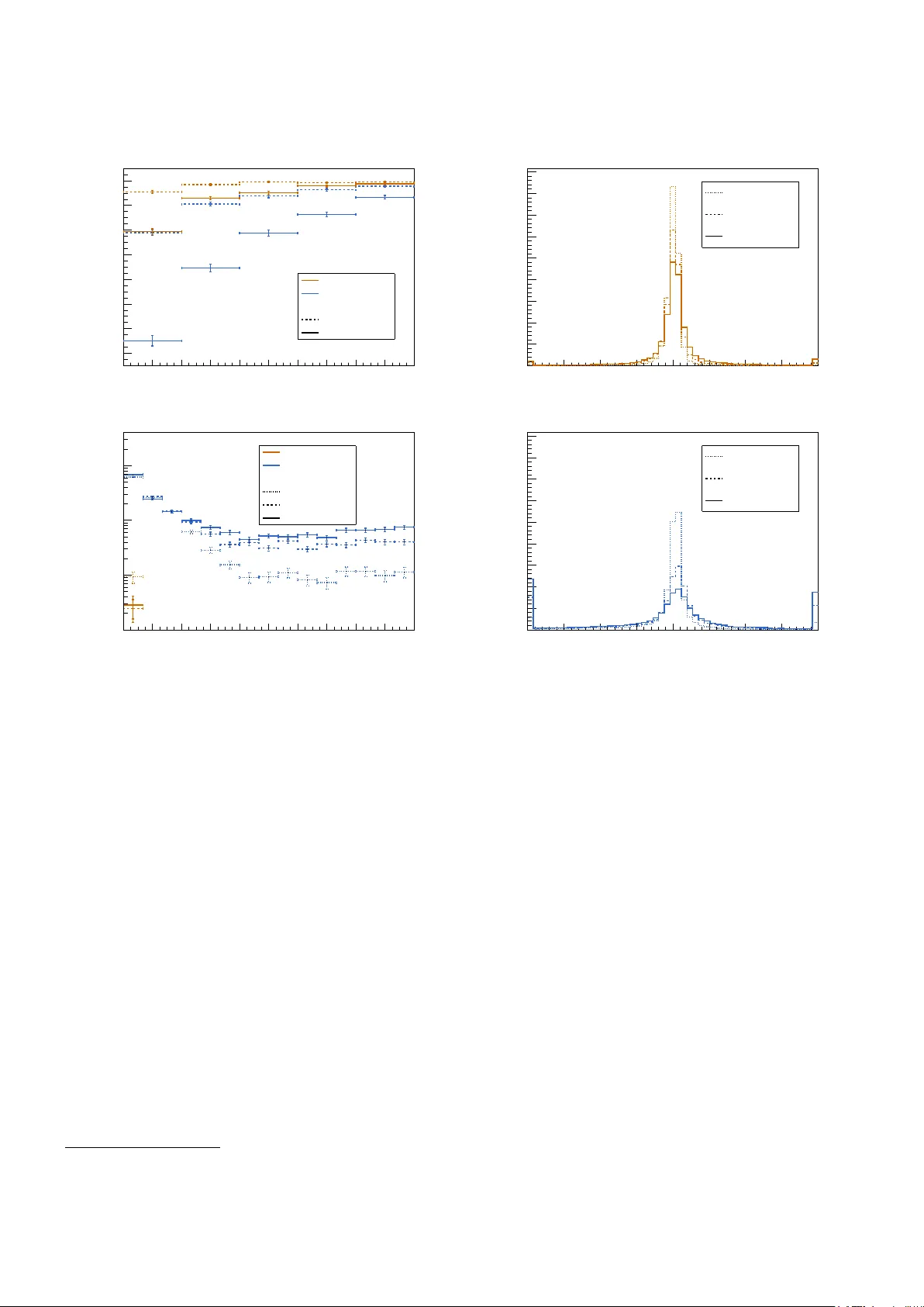
j (r)/

0 . 5 . The bottom plots only con tain jets not falling into this category . Left: mean of the jet momen tum resp onse. Righ t: width of the jet momentum resp onse. All distributions are shown for differen t fractions of c harged particles associated to pileup (PU frac.). All distributions are sho wn as a function of the true jet momentum. References 1. J. Redmon, S. K. Divv ala, R. B. Girshick, A. F arhadi, “Y ou Only Lo ok Once: Unified, Real-Time Ob ject Detection,” CoRR , abs/1506.02640 (2015), 1506.02640 , URL http:// arxiv.org/abs/1506.02640 . 2. J. Redmon, A. F arhadi, “ YOLO9000: Better, F aster, Stronger,” CoRR , abs/1612.08242 (2016), 1612.08242 , URL . 3. S. Ren, K. He, R. B. Girshic k, J. Sun, “F aster R-CNN: T o- w ards Real-Time Ob ject Detection with Region Prop osal Net works,” CoRR , abs/1506.01497 (2015), 1506.01497 , URL . 4. W. Liu, D. Anguelo v, D. Erhan, C. Szegedy , et al., “ SSD: Single Shot MultiBo x Detector,” CoRR , abs/1512.02325 (2015), 1512.02325 , URL 02325 . 5. T. Lin, P . Go yal, R. B. Girshic k, K. He, et al., “F ocal Loss for Dense Ob ject Detection,” CoRR , abs/1708.02002 (2017), 1708.02002 , URL http://arxiv.org/abs/1708.02002 . 6. K. He, G. Gkio xari, P . Dollár, R. B. Girshic k, “Mask R- CNN,” CoRR , abs/1703.06870 (2017), 1703.06870 , URL http://arxiv.org/abs/1703.06870 . 7. S. Shi, X. W ang, H. Li, “Poin tRCNN: 3D Ob ject Pro- p osal Generation and Detection from P oint Cloud,” CoRR , abs/1812.04244 (2018), 1812.04244 , URL http://arxiv. org/abs/1812.04244 . 8. C. Zh u, Y. He, M. Savvides, “F eature Selectiv e Anc hor- F ree Module for Single-Shot Ob ject Detection,” CoRR , abs/1903.00621 (2019), 1903.00621 , URL http://arxiv. org/abs/1903.00621 . 9. Z. Tian, C. Shen, H. Chen, T. He, “ FCOS: F ully Con v olu- tional One-Stage Ob ject Detection,” CoRR , abs/1904.01355 (2019), 1904.01355 , URL 01355 . 10. X. Zhou, D. W ang, P . Krähenbühl, “Ob jects as P oints,” CoRR , abs/1904.07850 (2019), 1904.07850 , URL http:// arxiv.org/abs/1904.07850 . 11. B. Li, Y. Liu, X. W ang, “Gradien t Harmonized Single- Stage Detector,” Pr o c e e dings of the AAAI Confer enc e on Artificial Intel ligenc e , 33 8577 (2019), doi:10.1609/aaai. v33i01.33018577. 12. N. Bodla, B. Singh, R. Chellappa, L. Davis, “Improv- ing Ob ject Detection With One Line of Co de,” CoRR , abs/1704.04503 (2017), 1704.04503 , URL http://arxiv. org/abs/1704.04503 . 13. M. Ruan, H. Videau, “ Arbor, a new approach of the P article Flo w Algorithm,” “ Pro ceedings, International Conference on Calorimetry for the High Energy F rontier (CHEF 2013): Jan Kiesele r: Ob ject condensation 11 P aris, F rance, April 22-25, 2013,” 316–324 (2013), 1403. 4784 . 14. M. Thomson, “P article flow calorimetry and the Pan- doraPF A algorithm,” Nucle ar Instruments and Metho ds in Physics R ese ar ch Se ction A: A c c eler ators, Sp e ctr om- eters, Dete ctors and Associate d Equipment , 611 25–40 (2009), ISSN 0168-9002, doi:10.1016/j.nima.2009.09.009, URL http://dx.doi.org/10.1016/j.nima.2009.09.009 . 15. J. Marshall, A. Münnic h, M. Thomson, “Performa nce of particle flo w calorimetry at CLIC,” Nucle ar Instruments and Metho ds in Physics R esea r ch Se ction A: A c c eler ators, Sp e ctr ometers, Dete ctors and Asso ciate d Equipment , 700 153–162 (2013), ISSN 0168-9002, doi:10.1016/j.nima.2012. 10.038, URL http://dx.doi.org/10.1016/j.nima.2012. 10.038 . 16. J. S. Marshall, M. A. Thomson, “ P andora Particle Flo w Algorithm,” “ Pro ceedings, International Conference on Calorimetry for the High Energy F rontier (CHEF 2013): P aris, F rance, April 22-25, 2013,” 305–315 (2013), 1308. 4537 . 17. J. S. Marshall, M. A. Thomson, “The P andora soft ware dev elopment kit for pattern recognition,” The Eur op e an Physic al Journal C , 75 (2015), ISSN 1434-6052, doi:10. 1140/ep jc/s10052- 015- 3659- 3, URL http://dx.doi.org/ 10.1140/epjc/s10052- 015- 3659- 3 . 18. F. Sefko w, A. White, K. Kaw ago e, R. Pösc hl, J. Re- p ond, “Exp erimental tests of particle flo w calorimetry ,” R eviews of Mo dern Physics , 88 (2016), ISSN 1539-0756, doi:10.1103/revmo dph ys.88.015003, URL http://dx.doi. org/10.1103/RevModPhys.88.015003 . 19. H. L. T ran, K. Krüger, F. Sefk o w, S. Green, J. Mar- shall, M. Thomson, F. Simon, “Soft ware compensation in particle flow reconstruction,” The Eur op e an Physic al Journal C , 77 (2017), ISSN 1434-6052, doi:10.1140/ep jc/ s10052- 017- 5298- 3, URL http://dx.doi.org/10.1140/ epjc/s10052- 017- 5298- 3 . 20. L. Ev ans, P . Bry ant, “ LHC Mac hine,” Journal of Instru- mentation , 3 S08001 (2008), doi:10.1088/1748- 0221/3/08/ s08001, URL https://doi.org/10.1088%2F1748- 0221% 2F3%2F08%2Fs08001 . 21. CMS Collab oration, “P article-flo w reconstruction and global even t description with the CMS detector,” Journal of Instrumentation , 12 P10003–P10003 (2017), ISSN 1748- 0221, doi:10.1088/1748- 0221/12/10/p10003, URL http: //dx.doi.org/10.1088/1748- 0221/12/10/P10003 . 22. A TLAS Collab oration (A TLAS), “ Jet reconstruction and p erformance using particle flow with the A TLAS De- tector,” Eur. Phys. J. , C77 (2017), doi:10.1140/ep jc/ s10052- 017- 5031- 2, 1703.10485 . 23. D. Guest, K. Cranmer, D. Whiteson, “ Deep Learning and its Application to LHC Ph ysics,” A nn. R ev. Nucl. Part. Sci. , 68 (2018), doi:10.1146/annurev- nucl- 101917- 021019, 1806.11484 . 24. L. de Oliveira, B. Nachman, M. Paganini, “Electromagnetic sho wers b eyond show er shapes,” Nucle ar Instruments and Metho ds in Physics R ese ar ch Se ction A: A c c eler ators, Sp e c- tr ometers, Dete ctors and Asso ciate d Equipment , 951 162879 (2020), ISSN 0168-9002, doi:10.1016/j.nima.2019.162879, URL http://dx.doi.org/10.1016/j.nima.2019.162879 . 25. D. Belayneh, F. Carminati, A. F arbin, B. Hoob erman, et al., “Calorimetry with deep learning: particle classification, en- ergy regression, and simulation for high-energy ph ysics,” (2019), 1912.06794 . 26. P . K omiske, E. Meto diev, B. Nac hman, M. Sc hw artz, “Pileup Mitigation with Mac hine Learning (PUMML),” Journal of High Ener gy Physics , 2017 (2017), ISSN 1029- 8479, doi:10.1007/jhep12(2017)051, URL http://dx.doi. org/10.1007/JHEP12(2017)051 . 27. CMS Collab oration, “ CMS Phase 1 heavy flav our iden- tification p erformance and developmen ts,” (2017), URL https://cds.cern.ch/record/2263802 . 28. CMS Collab oration, “ New Developmen ts for Jet Sub- structure Reconstruction in CMS,” (2017), URL https: //cds.cern.ch/record/2275226 . 29. A TLAS Collaboration, “ Iden tification of Jets Con taining b -Hadrons with Recurrent Neural Net w orks at the A TLAS Exp erimen t,” (2017), URL https://cds.cern.ch/record/ 2255226 . 30. T. Q. Nguy en, et al., “ T opology classification with deep learning to improv e real-time even t selection at the LHC,” (2018), arXiv:1807.00083 [hep-ex]. 31. A. Butter, K. Cranmer, D. Debnath, B. M. Dillon, et al., “ The Mac hine Learning Landscap e of T op T aggers,” Sci- Post Phys. , 7 014 (2019), doi:10.21468/SciPostPh ys.7.1.014, 1902.09914 . 32. F. Scarselli, M. Gori, A. T soi, M. Hagenbuc hner, et al., “The graph neural net w ork model,” IEEE T r ansactions on Neur al Networks , 20 (2009). 33. S. Qasim, J. Kieseler, Y. Iiyama, M. Pierini, “ Learning represen tations of irregular particle-detector geometry with distance-w eighted graph netw orks,” Eur. Phys. J. , C79 608 (2019), doi:10.1140/ep jc/s10052- 019- 7113- 9, 1902.07987 . 34. E. Moreno, O. Cerri, J. Duarte, H. Newman, et al., “ JEDI- net: a jet iden tification algorithm based on in teraction net works,” Eur. Phys. J. , C80 58 (2020), doi:10.1140/ep jc/ s10052- 020- 7608- 4, 1908.05318 . 35. H. Qu, L. Gousk os, “ P articleNet: Jet T agging via Particle Clouds,” (2019), 1902.08570 . 36. S. F arrell, P . Calafiura, M. Mudigonda, Prabhat, et al., “ Nov el deep learning metho ds for track reconstruction,” “ 4th International W orkshop Connecting The Dots 2018 (CTD2018) Seattle, W ashington, USA, Marc h 20-22, 2018,” (2018), 1810.06111 , URL http://lss.fnal.gov/archive/ 2018/conf/fermilab- conf- 18- 598- cd.pdf . 37. S. F arrel, D. Anderson, P . Calafiura, G. Cerati, et al., “The HEP .T rkX Pro ject: deep neural netw orks for HL-LHC online and offline trac king,” EPJ W eb Conf. , 150 00003 (2017), doi:10.1051/ep jconf/201715000003, URL https:// doi.org/10.1051/epjconf/201715000003 . 38. X. Ju, S. F arrell, P . Calafiura, D. Murnane, et al., “ Graph Neural Net w orks for P article Reconstruction in High Energy Ph ysics detectors,” “ Thirt y-third Conference on Neural In- formation Pro cessing Systems (NeurIPS2019), V ancouver, Canada,” (2019), URL https://ml4physicalsciences. github.io/files/NeurIPS_ML4PS_2019_83.pdf . 39. D. Neven, B. D. Brabandere, M. Pro esmans, L. V. Go ol, “In- stance Segmentation by Jointly Optimizing Spatial Embed- dings and Clustering Bandwidth,” CoRR , abs/1906.11109 (2019), 1906.11109 , URL 11109 . 40. B. Zhang, P . W onk a, “P oint Cloud Instance Segmentation using Probabilistic Em b eddings,” ArXiv , abs/1912.00145 (2019). 41. S. v an der W alt, J. Schön berger, J. Nunez-Iglesias, F. Boulogne, et al., “scikit-image: image pro cessing in Python,” Pe erJ , 2 e453 (2014), ISSN 2167-8359, doi:10. 12 Jan Kieseler: Ob ject condensation 7717/p eerj.453, URL https://doi.org/10.7717/peerj. 453 . 42. Y. LeCun, L. Bottou, Y. Bengio, P . Haffner, “Gradien t- Based Learning Applied to Document Recognition,” “Intel- ligen t Signal Pro cessing,” 306–351, IEEE Press (2001). 43. D.-A. Clevert, T. Un terthiner, S. Ho c hreiter, “ F ast and A ccurate Deep Net work Learning by Exponential Linear Units (ELUs),” (2015), 1511.07289 . 44. M. Abadi, A. Agarwal, P . Barham, E. Brevdo, Z. Chen, C. Citro, other, “ T ensorFlow: Large-Scale Machine Learning on Heterogeneous Systems,” (2015), softw are av ailable from tensorflo w.org, URL https://www.tensorflow.org/ . 45. F. Chollet, et al., “Keras,” (2015), URL https://github. com/fchollet/keras . 46. J. Kieseler, M. Stoy e, M. V erzetti, P . Silv a, S. S. Meh ta, A. Stakia, Y. Iiy ama, E. Bols, S. R. Qasim, H. Kirsc hen- mann, et al., “DeepJetCore,” (2020), doi:10.5281/zenodo. 3670882. 47. D. P . Kingma, J. Ba, “Adam: A Metho d for Sto c hastic Optimization,” “3rd In ternational Conference on Learning Represen tations, ICLR 2015, San Diego, CA, USA, May 7-9, 2015, Conference T rack Pro ceedings,” (2015), URL http://arxiv.org/abs/1412.6980 . 48. Y. Nestero v, “A metho d of solving a conv ex programming problem with conv ergence rate O (1 /k 2 ) ,” Soviet Mathemat- ics. Doklady , 27 372 (1983). 49. T. Dozat, “Incorp orating Nesterov Momentum into Adam,” Pr o c ee dings of the International Confer enc e on L e arning R epr esentations 2016 (2016). 50. L. N. Smith, “No More P esky Learning Rate Guessing Games,” CoRR , abs/1506.01186 (2015), 1506.01186 , URL http://arxiv.org/abs/1506.01186 . 51. F. A. D. Bello, S. Ganguly , E. Gross, M. Kado, M. Pitt, J. Shlomi, L. Santi, “T ow ards a Computer Vision Particle Flo w,” (2020), 2003.08863 . 52. A. Abada, et al., “FCC-hh: The Hadron Collider,” The Eu- r op e an Physic al Journal Sp e cial T opics , 228 755 (2019), doi: 10.1140/ep jst/e2019- 900087- 0, URL https://doi.org/10. 1140/epjst/e2019- 900087- 0 . 53. M. Aleksa, P . Allport, R. Bosley , J. F altov a, J. Gen til, R. Goncalo, C. Helsens, A. Henriques, A. Karyukhin, J. Kieseler, C. Neubüser, H. F. P . D. Silv a, T. Price, J. Sc hliwinski, M. Selv aggi, O. Solovy anov, A. Zab oro wsk a, “Calorimeters for the FCC-hh,” (2019), 1912.09962 . 54. CMS Collab oration, “ The Phase-2 Upgrade of the CMS Endcap Calorimeter,” T echnical Rep ort CERN-LHCC-2017- 023. CMS-TDR-019 (2017), URL https://cds.cern.ch/ record/2293646 . 55. S. Agostinelli, et al. (GEANT4), “ GEANT4: A Simulation to olkit,” Nucl. Instrum. Meth. , A506 (2003), doi:10.1016/ S0168- 9002(03)01368- 8. 56. CMS Collab oration (CMS), “The CMS exp eriment at the CERN LHC,” JINST , 3 S08004 (2008), doi:10.1088/ 1748- 0221/3/08/S08004.