Tomographic and entropic analysis of modulated signals

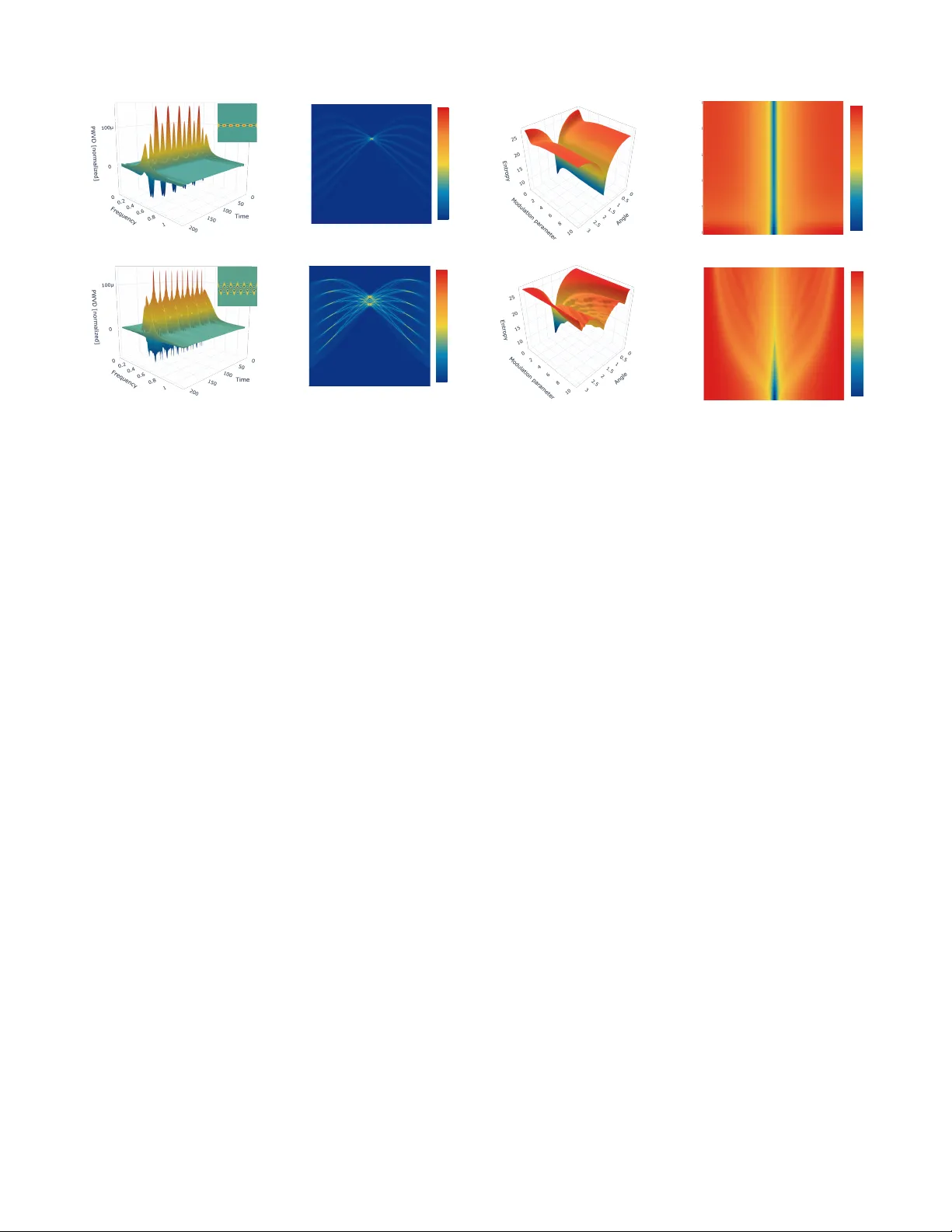
T omographic and en tropic analysis of mo dulated signals A.S. Mastiuk ov a, 1, 2 M.A. Ga vreev, 1, 2 E.O. Kiktenk o, 1, 2, 3 and A.K. F edoro v 1, 2 1 Russian Quantum Center, Skolkovo, Mosc ow 143025, Russia 2 Mosc ow Institute of Physics and T e chnolo gy, Dolgoprudny, Mosc ow R e gion 141700, Russia 3 Dep artment of Mathematic al Metho ds for Quantum T e chnolo gies, Steklov Mathematic al Institute of Russian A c ademy of Sciences, Mosc ow 119991, Russia (Dated: Septem b er 29, 2020) W e study an application of the quantum tomography framew ork for the time-frequency analysis of mo dulated signals. In particular, we calculate optical tomographic represen tations and Wigner-Ville distributions for signals with amplitude and frequency modulations. W e also consider t ime-frequency en tropic relations for mo dulated signals, which are naturally associated with the F ourier analysis. A n umerical to olbox for calculating optical time-frequency tomograms based on pseudo Wigner-Ville distributions for mo dulated signals is provided. I. INTR ODUCTION Time-frequency analysis is a pow erful to ol of modern signal processing [ 1 – 4 ]. Complemen tary to the informa- tion that can be extracted from the frequency domain via F ourier analysis, time-frequency analysis pro vides a wa y for studying a signal in b oth time and frequency repre- sen tations simultaneously . This is useful, in particular, for signals of a sophisticated structure that change signifi- can tly ov er their duration, for example, m usic signals [ 5 ]. Existing approaches to time-frequency analysis use lin- ear canonical transformations preserving the symplectic form [ 1 ]. Geometrically this can b e illustrated as follows: the F ourier transform can b e view ed as a π / 2 rotation in the asso ciated time-frequency plane, whereas other time-frequency representations allo w arbitrary symplec- tic transformations in the time-frequency plane. There is a num b er of wa ys for defining a time-frequency distribu- tion function with required properties (for a review, see Ref. [ 4 ]). T ransformations b et ween v arious distributions in time-frequency analysis are quite well-understoo d [ 1 ]. The idea behind time-frequency analysis is v ery close to the motiv ation for studying phase-space representa- tions in quantum physics. As it is w ell known, the re- lation b et ween position and momentum represen tations of the wa v e function is giv en b y the F ourier transform, whic h is similar to the relation betw een signals in time and frequency domains. This analogy b ecomes ev en more transparen t in the framework of analytic signals, which are complex as well as wa v e functions. One of the possible w ays to characterize a quantum state in the phase space are to use the Wigner quasiprobabilit y distribution [ 6 ]. The Wigner quasiprobability distribution resem bles clas- sical phase space probability distributions that is used in statistical mec hanics. How ev er, it cannot b e fully inter- preted as a probability distribution since it takes nega- tiv e v alues [ 6 – 8 ]. W e also note the Wigner quasiprobabil- it y distribution is successfully used for analyzing v arious phenomena in quantum optics and quantum statistical ph ysics [ 8 ]. In the field of signal pro cessing, the Wigner distribution function often referred to as the Wigner– Ville distribution [ 9 , 10 ]. The application of the Wigner distribution mak es an in teresting connection b et ween the metho ds in quantum physics and signal pro cessing, es- p ecially in the context of time-frequency and p osition- momen tum uncertaint y relations. Recen t decades, the link b et ween phase space form ula- tion of quan tum mec hanics and time-frequency analysis in tensively studied in the context of quan tum tomogra- ph y [ 11 ]. Quan tum tomography appears as a tec hnique for the reconstruction of the Wigner function (densit y matrix) in quantum-optical exp erimen ts [ 12 ]. The re- sults of tomographic measurements in principle contain all the information ab out the measured system, so they can b e considered as a quantities for the description of quan tum states [ 11 ]. This is the core idea b ehind the omographic representation of quantum states. In par- ticular, symplectic tomography proto cols use a marginal probabilit y distribution of shifted and squeezed p osition and momentum v ariables. This approac h has b een used in the con text of time-frequency analysis [ 13 ] and time- frequency en tropic analysis [ 14 ] for v arious t ypes of sig- nals, suc h as complex Gaussian signals [ 13 – 18 ] and reflec- tometry data [ 19 , 20 ]. A general analysis of the relation b et w een time-frequency tomograms and other transfor- mations (including w av elets) is presented in Ref. [ 15 ]. Ho wev er, the considered examples of signals lack ana- lyzing mo dulated signals, which are intensiv ely used in telecomm unication signals. Moreov er, the Wigner-Ville distribution has been considered in the con text of diag- nostics of features of mo dulated signals [ 21 ], so one can exp ect that tomograms are helpful for such an analysis. In this work, we consider tomographic representations for mo dulated signals. W e calculate optical tomographic represen tations and Wigner-Ville distributions for signals with amplitude and frequency m odulations. In particu- lar, we study the method of the optical time-frequency tomograms via pseudo Wigner-Ville distributions, and discuss adv antages of suc h an approach. W e also consider time-frequency en tropic relations for mo dulated signals. Our work is organized as follo ws. In Sec. I I , w e in tro- duce general relations for tomographic analysis of ana- lytic signals. In Sec. I II , w e calculate optical tomographic represen tations for signals with amplitude and frequency 2  0 1 0 0 1 2 0 0 . 3 5 0 . 4 0 . 4 5 0 . 5 0 . 5 5 0 . 6 0 2 0 0  4 0 0  6 0 0   0 0   0  0 1 0 0 1 1 0 1 2 0 0 . 3 5 0 . 4 0 . 4 5 0 . 5 0 . 5 5 0 . 6 0 0 . 0 0 0 2 0 . 0 0 0 4 0 . 0 0 0 6 0 . 0 0 0  0 . 0 0 1 0 100 120 0 . 3 5 0 . 4 0 . 4 5 0 . 5 0 . 5 5 0 . 6 0 5 10 15 20 25 0 1 2  0 0.0 0.1 0.1 0 1 2  0 0.0 0.1 0.1 0 1 2  0 0.001 0.002 0.00 0.00 0.00 (a) (c) (d) (e) (f) (b) ✓ AAAB7XicbVBNS8NAEJ3Ur1q/qh69LBbBU0mqoMeiF48V7Ae0oWy2m3btZhN2J0IJ/Q9ePCji1f/jzX/jts1BWx8MPN6bYWZekEhh0HW/ncLa+sbmVnG7tLO7t39QPjxqmTjVjDdZLGPdCajhUijeRIGSdxLNaRRI3g7GtzO//cS1EbF6wEnC/YgOlQgFo2ilVg9HHGm/XHGr7hxklXg5qUCORr/81RvELI24QiapMV3PTdDPqEbBJJ+WeqnhCWVjOuRdSxWNuPGz+bVTcmaVAQljbUshmau/JzIaGTOJAtsZURyZZW8m/ud1Uwyv/UyoJEWu2GJRmEqCMZm9TgZCc4ZyYgllWthbCRtRTRnagEo2BG/55VXSqlW9i2rt/rJSv8njKMIJnMI5eHAFdbiDBjSBwSM8wyu8ObHz4rw7H4vWgpPPHMMfOJ8/pUWPLA== ✓ AAAB7XicbVBNS8NAEJ3Ur1q/qh69LBbBU0mqoMeiF48V7Ae0oWy2m3btZhN2J0IJ/Q9ePCji1f/jzX/jts1BWx8MPN6bYWZekEhh0HW/ncLa+sbmVnG7tLO7t39QPjxqmTjVjDdZLGPdCajhUijeRIGSdxLNaRRI3g7GtzO//cS1EbF6wEnC/YgOlQgFo2ilVg9HHGm/XHGr7hxklXg5qUCORr/81RvELI24QiapMV3PTdDPqEbBJJ+WeqnhCWVjOuRdSxWNuPGz+bVTcmaVAQljbUshmau/JzIaGTOJAtsZURyZZW8m/ud1Uwyv/UyoJEWu2GJRmEqCMZm9TgZCc4ZyYgllWthbCRtRTRnagEo2BG/55VXSqlW9i2rt/rJSv8njKMIJnMI5eHAFdbiDBjSBwSM8wyu8ObHz4rw7H4vWgpPPHMMfOJ8/pUWPLA== ✓ AAAB7XicbVBNS8NAEJ3Ur1q/qh69LBbBU0mqoMeiF48V7Ae0oWy2m3btZhN2J0IJ/Q9ePCji1f/jzX/jts1BWx8MPN6bYWZekEhh0HW/ncLa+sbmVnG7tLO7t39QPjxqmTjVjDdZLGPdCajhUijeRIGSdxLNaRRI3g7GtzO//cS1EbF6wEnC/YgOlQgFo2ilVg9HHGm/XHGr7hxklXg5qUCORr/81RvELI24QiapMV3PTdDPqEbBJJ+WeqnhCWVjOuRdSxWNuPGz+bVTcmaVAQljbUshmau/JzIaGTOJAtsZURyZZW8m/ud1Uwyv/UyoJEWu2GJRmEqCMZm9TgZCc4ZyYgllWthbCRtRTRnagEo2BG/55VXSqlW9i2rt/rJSv8njKMIJnMI5eHAFdbiDBjSBwSM8wyu8ObHz4rw7H4vWgpPPHMMfOJ8/pUWPLA== ⇡ AAAB6nicbVBNS8NAEJ3Ur1q/qh69LBbBU0mqoMeiF48V7Qe0oWy2k3bpZhN2N0IJ/QlePCji1V/kzX/jts1BWx8MPN6bYWZekAiujet+O4W19Y3NreJ2aWd3b/+gfHjU0nGqGDZZLGLVCahGwSU2DTcCO4lCGgUC28H4dua3n1BpHstHM0nQj+hQ8pAzaqz00Et4v1xxq+4cZJV4OalAjka//NUbxCyNUBomqNZdz02Mn1FlOBM4LfVSjQllYzrErqWSRqj9bH7qlJxZZUDCWNmShszV3xMZjbSeRIHtjKgZ6WVvJv7ndVMTXvsZl0lqULLFojAVxMRk9jcZcIXMiIkllClubyVsRBVlxqZTsiF4yy+vklat6l1Ua/eXlfpNHkcRTuAUzsGDK6jDHTSgCQyG8Ayv8OYI58V5dz4WrQUnnzmGP3A+fwBRC43R ⇡ AAAB6nicbVBNS8NAEJ3Ur1q/qh69LBbBU0mqoMeiF48V7Qe0oWy2k3bpZhN2N0IJ/QlePCji1V/kzX/jts1BWx8MPN6bYWZekAiujet+O4W19Y3NreJ2aWd3b/+gfHjU0nGqGDZZLGLVCahGwSU2DTcCO4lCGgUC28H4dua3n1BpHstHM0nQj+hQ8pAzaqz00Et4v1xxq+4cZJV4OalAjka//NUbxCyNUBomqNZdz02Mn1FlOBM4LfVSjQllYzrErqWSRqj9bH7qlJxZZUDCWNmShszV3xMZjbSeRIHtjKgZ6WVvJv7ndVMTXvsZl0lqULLFojAVxMRk9jcZcIXMiIkllClubyVsRBVlxqZTsiF4yy+vklat6l1Ua/eXlfpNHkcRTuAUzsGDK6jDHTSgCQyG8Ayv8OYI58V5dz4WrQUnnzmGP3A+fwBRC43R ⇡ AAAB6nicbVBNS8NAEJ3Ur1q/qh69LBbBU0mqoMeiF48V7Qe0oWy2k3bpZhN2N0IJ/QlePCji1V/kzX/jts1BWx8MPN6bYWZekAiujet+O4W19Y3NreJ2aWd3b/+gfHjU0nGqGDZZLGLVCahGwSU2DTcCO4lCGgUC28H4dua3n1BpHstHM0nQj+hQ8pAzaqz00Et4v1xxq+4cZJV4OalAjka//NUbxCyNUBomqNZdz02Mn1FlOBM4LfVSjQllYzrErqWSRqj9bH7qlJxZZUDCWNmShszV3xMZjbSeRIHtjKgZ6WVvJv7ndVMTXvsZl0lqULLFojAVxMRk9jcZcIXMiIkllClubyVsRBVlxqZTsiF4yy+vklat6l1Ua/eXlfpNHkcRTuAUzsGDK6jDHTSgCQyG8Ayv8OYI58V5dz4WrQUnnzmGP3A+fwBRC43R 0 AAAB6HicbVBNS8NAEJ3Ur1q/qh69LBbBU0mqoMeiF48t2FpoQ9lsJ+3azSbsboQS+gu8eFDEqz/Jm//GbZuDtj4YeLw3w8y8IBFcG9f9dgpr6xubW8Xt0s7u3v5B+fCoreNUMWyxWMSqE1CNgktsGW4EdhKFNAoEPgTj25n/8IRK81jem0mCfkSHkoecUWOlptsvV9yqOwdZJV5OKpCj0S9/9QYxSyOUhgmqdddzE+NnVBnOBE5LvVRjQtmYDrFrqaQRaj+bHzolZ1YZkDBWtqQhc/X3REYjrSdRYDsjakZ62ZuJ/3nd1ITXfsZlkhqUbLEoTAUxMZl9TQZcITNiYgllittbCRtRRZmx2ZRsCN7yy6ukXat6F9Va87JSv8njKMIJnMI5eHAFdbiDBrSAAcIzvMKb8+i8OO/Ox6K14OQzx/AHzucPemeMuA== 0 AAAB6HicbVBNS8NAEJ3Ur1q/qh69LBbBU0mqoMeiF48t2FpoQ9lsJ+3azSbsboQS+gu8eFDEqz/Jm//GbZuDtj4YeLw3w8y8IBFcG9f9dgpr6xubW8Xt0s7u3v5B+fCoreNUMWyxWMSqE1CNgktsGW4EdhKFNAoEPgTj25n/8IRK81jem0mCfkSHkoecUWOlptsvV9yqOwdZJV5OKpCj0S9/9QYxSyOUhgmqdddzE+NnVBnOBE5LvVRjQtmYDrFrqaQRaj+bHzolZ1YZkDBWtqQhc/X3REYjrSdRYDsjakZ62ZuJ/3nd1ITXfsZlkhqUbLEoTAUxMZl9TQZcITNiYgllittbCRtRRZmx2ZRsCN7yy6ukXat6F9Va87JSv8njKMIJnMI5eHAFdbiDBrSAAcIzvMKb8+i8OO/Ox6K14OQzx/AHzucPemeMuA== 0 AAAB6HicbVBNS8NAEJ3Ur1q/qh69LBbBU0mqoMeiF48t2FpoQ9lsJ+3azSbsboQS+gu8eFDEqz/Jm//GbZuDtj4YeLw3w8y8IBFcG9f9dgpr6xubW8Xt0s7u3v5B+fCoreNUMWyxWMSqE1CNgktsGW4EdhKFNAoEPgTj25n/8IRK81jem0mCfkSHkoecUWOlptsvV9yqOwdZJV5OKpCj0S9/9QYxSyOUhgmqdddzE+NnVBnOBE5LvVRjQtmYDrFrqaQRaj+bHzolZ1YZkDBWtqQhc/X3REYjrSdRYDsjakZ62ZuJ/3nd1ITXfsZlkhqUbLEoTAUxMZl9TQZcITNiYgllittbCRtRRZmx2ZRsCN7yy6ukXat6F9Va87JSv8njKMIJnMI5eHAFdbiDBrSAAcIzvMKb8+i8OO/Ox6K14OQzx/AHzucPemeMuA== X AAAB6HicbVBNS8NAEJ3Ur1q/qh69LBbBU0mqoMeiF48t2FpoQ9lsJ+3azSbsboQS+gu8eFDEqz/Jm//GbZuDtj4YeLw3w8y8IBFcG9f9dgpr6xubW8Xt0s7u3v5B+fCoreNUMWyxWMSqE1CNgktsGW4EdhKFNAoEPgTj25n/8IRK81jem0mCfkSHkoecUWOlZqdfrrhVdw6ySrycVCBHo1/+6g1ilkYoDRNU667nJsbPqDKcCZyWeqnGhLIxHWLXUkkj1H42P3RKzqwyIGGsbElD5urviYxGWk+iwHZG1Iz0sjcT//O6qQmv/YzLJDUo2WJRmApiYjL7mgy4QmbExBLKFLe3EjaiijJjsynZELzll1dJu1b1Lqq15mWlfpPHUYQTOIVz8OAK6nAHDWgBA4RneIU359F5cd6dj0VrwclnjuEPnM8ftweM4A== X AAAB6HicbVBNS8NAEJ3Ur1q/qh69LBbBU0mqoMeiF48t2FpoQ9lsJ+3azSbsboQS+gu8eFDEqz/Jm//GbZuDtj4YeLw3w8y8IBFcG9f9dgpr6xubW8Xt0s7u3v5B+fCoreNUMWyxWMSqE1CNgktsGW4EdhKFNAoEPgTj25n/8IRK81jem0mCfkSHkoecUWOlZqdfrrhVdw6ySrycVCBHo1/+6g1ilkYoDRNU667nJsbPqDKcCZyWeqnGhLIxHWLXUkkj1H42P3RKzqwyIGGsbElD5urviYxGWk+iwHZG1Iz0sjcT//O6qQmv/YzLJDUo2WJRmApiYjL7mgy4QmbExBLKFLe3EjaiijJjsynZELzll1dJu1b1Lqq15mWlfpPHUYQTOIVz8OAK6nAHDWgBA4RneIU359F5cd6dj0VrwclnjuEPnM8ftweM4A== X AAAB6HicbVBNS8NAEJ3Ur1q/qh69LBbBU0mqoMeiF48t2FpoQ9lsJ+3azSbsboQS+gu8eFDEqz/Jm//GbZuDtj4YeLw3w8y8IBFcG9f9dgpr6xubW8Xt0s7u3v5B+fCoreNUMWyxWMSqE1CNgktsGW4EdhKFNAoEPgTj25n/8IRK81jem0mCfkSHkoecUWOlZqdfrrhVdw6ySrycVCBHo1/+6g1ilkYoDRNU667nJsbPqDKcCZyWeqnGhLIxHWLXUkkj1H42P3RKzqwyIGGsbElD5urviYxGWk+iwHZG1Iz0sjcT//O6qQmv/YzLJDUo2WJRmApiYjL7mgy4QmbExBLKFLe3EjaiijJjsynZELzll1dJu1b1Lqq15mWlfpPHUYQTOIVz8OAK6nAHDWgBA4RneIU359F5cd6dj0VrwclnjuEPnM8ftweM4A== t AAAB6HicbVBNS8NAEJ3Ur1q/qh69LBbBU0mqoMeiF48t2FpoQ9lsN+3azSbsToQS+gu8eFDEqz/Jm//GbZuDtj4YeLw3w8y8IJHCoOt+O4W19Y3NreJ2aWd3b/+gfHjUNnGqGW+xWMa6E1DDpVC8hQIl7ySa0yiQ/CEY3878hyeujYjVPU4S7kd0qEQoGEUrNbFfrrhVdw6ySrycVCBHo1/+6g1ilkZcIZPUmK7nJuhnVKNgkk9LvdTwhLIxHfKupYpG3PjZ/NApObPKgISxtqWQzNXfExmNjJlEge2MKI7MsjcT//O6KYbXfiZUkiJXbLEoTCXBmMy+JgOhOUM5sYQyLeythI2opgxtNiUbgrf88ipp16reRbXWvKzUb/I4inACp3AOHlxBHe6gAS1gwOEZXuHNeXRenHfnY9FacPKZY/gD5/MH4XeM/A== ! AAAB7XicbVDLSgNBEJyNrxhfUY9eBoPgKexGQY9BLx4jmAckS5id9CZj5rHMzAphyT948aCIV//Hm3/jJNmDJhY0FFXddHdFCWfG+v63V1hb39jcKm6Xdnb39g/Kh0cto1JNoUkVV7oTEQOcSWhaZjl0Eg1ERBza0fh25refQBum5IOdJBAKMpQsZpRYJ7V6SsCQ9MsVv+rPgVdJkJMKytHol796A0VTAdJSTozpBn5iw4xoyyiHaamXGkgIHZMhdB2VRIAJs/m1U3zmlAGOlXYlLZ6rvycyIoyZiMh1CmJHZtmbif953dTG12HGZJJakHSxKE45tgrPXscDpoFaPnGEUM3crZiOiCbUuoBKLoRg+eVV0qpVg4tq7f6yUr/J4yiiE3SKzlGArlAd3aEGaiKKHtEzekVvnvJevHfvY9Fa8PKZY/QH3ucPkX+PHw== T ( X, ✓ ) AAAB/nicbVDLSsNAFJ34rPUVFVduBotQQUpSBV0W3bis0Bc0oUymk3boZBJmboQSCv6KGxeKuPU73Pk3TtoutPXAwOGce7lnTpAIrsFxvq2V1bX1jc3CVnF7Z3dv3z44bOk4VZQ1aSxi1QmIZoJL1gQOgnUSxUgUCNYORne5335kSvNYNmCcMD8iA8lDTgkYqWcfexGBISUia0zKnQsPhgzIec8uORVnCrxM3DkpoTnqPfvL68c0jZgEKojWXddJwM+IAk4FmxS9VLOE0BEZsK6hkkRM+9k0/gSfGaWPw1iZJwFP1d8bGYm0HkeBmczD6kUvF//zuimEN37GZZICk3R2KEwFhhjnXeA+V4yCGBtCqOImK6ZDoggF01jRlOAufnmZtKoV97JSfbgq1W7ndRTQCTpFZeSia1RD96iOmoiiDD2jV/RmPVkv1rv1MRtdseY7R+gPrM8fq+2VSg== T p ( X, ✓ ) AAACAHicbVBNS8NAEN34WetX1IMHL8EiVJCSVEGPRS8eK/QLmhA22027dLMJuxOhhF78K148KOLVn+HNf+OmzUFbHww83pthZl6QcKbAtr+NldW19Y3N0lZ5e2d3b988OOyoOJWEtknMY9kLsKKcCdoGBpz2EklxFHDaDcZ3ud99pFKxWLRgklAvwkPBQkYwaMk3j90Iw4hgnrWmflLtXbgwooDPfbNi1+wZrGXiFKSCCjR988sdxCSNqADCsVJ9x07Ay7AERjidlt1U0QSTMR7SvqYCR1R52eyBqXWmlYEVxlKXAGum/p7IcKTUJAp0Z36uWvRy8T+vn0J442VMJClQQeaLwpRbEFt5GtaASUqATzTBRDJ9q0VGWGICOrOyDsFZfHmZdOo157JWf7iqNG6LOEroBJ2iKnLQNWqge9REbUTQFD2jV/RmPBkvxrvxMW9dMYqZI/QHxucPQZiWLQ== D ( X, ✓ ) AAAB/nicbVDLSsNAFJ3UV62vqLhyM1iEClKSKuiyqAuXFewDmlAm02k7dDIJMzdCCQV/xY0LRdz6He78GydtFlo9MHA4517umRPEgmtwnC+rsLS8srpWXC9tbG5t79i7ey0dJYqyJo1EpDoB0UxwyZrAQbBOrBgJA8Hawfg689sPTGkeyXuYxMwPyVDyAacEjNSzD7yQwIgSkd5MK51TD0YMyEnPLjtVZwb8l7g5KaMcjZ796fUjmoRMAhVE667rxOCnRAGngk1LXqJZTOiYDFnXUElCpv10Fn+Kj43Sx4NImScBz9SfGykJtZ6EgZnMwupFLxP/87oJDC79lMs4ASbp/NAgERginHWB+1wxCmJiCKGKm6yYjogiFExjJVOCu/jlv6RVq7pn1drdebl+lddRRIfoCFWQiy5QHd2iBmoiilL0hF7Qq/VoPVtv1vt8tGDlO/voF6yPb5L9lTo= D ( t, ! ) AAAB/nicbVDLSgMxFM3UV62vUXHlJliEClJmqqDLoi5cVrAP6Awlk6ZtaB5DkhHKUPBX3LhQxK3f4c6/MdPOQqsHAodz7uWenChmVBvP+3IKS8srq2vF9dLG5tb2jru719IyUZg0sWRSdSKkCaOCNA01jHRiRRCPGGlH4+vMbz8QpakU92YSk5CjoaADipGxUs89CDgyI4xYejOtmNNAcjJEJz237FW9GeBf4uekDHI0eu5n0Jc44UQYzJDWXd+LTZgiZShmZFoKEk1ihMdoSLqWCsSJDtNZ/Ck8tkofDqSyTxg4U39upIhrPeGRnczC6kUvE//zuokZXIYpFXFiiMDzQ4OEQSNh1gXsU0WwYRNLEFbUZoV4hBTCxjZWsiX4i1/+S1q1qn9Wrd2dl+tXeR1FcAiOQAX44ALUwS1ogCbAIAVP4AW8Oo/Os/PmvM9HC06+sw9+wfn4Bqp6lUk= W p ( t, ! ) AAAB9HicbVDLSgNBEJyNrxhfUY9eFoMQQcJuFPQY9OIxgnlAsoTZyWwyZB7rTG8gLPkOLx4U8erHePNvnCR70MSChqKqm+6uMObMgOd9O7m19Y3Nrfx2YWd3b/+geHjUNCrRhDaI4kq3Q2woZ5I2gAGn7VhTLEJOW+Hobua3xlQbpuQjTGIaCDyQLGIEg5WCVi8uw0VXCTrA571iyat4c7irxM9ICWWo94pf3b4iiaASCMfGdHwvhiDFGhjhdFroJobGmIzwgHYslVhQE6Tzo6fumVX6bqS0LQnuXP09kWJhzESEtlNgGJplbyb+53USiG6ClMk4ASrJYlGUcBeUO0vA7TNNCfCJJZhoZm91yRBrTMDmVLAh+Msvr5JmteJfVqoPV6XabRZHHp2gU1RGPrpGNXSP6qiBCHpCz+gVvTlj58V5dz4WrTknmzlGf+B8/gDUbZF8 W ( t, ! ) AAAB8nicbVBNSwMxEM3Wr1q/qh69BItQQcpuFfRY9OKxgv2A7VKyabYNTTZLMiuUpT/DiwdFvPprvPlvTNs9aOuDgcd7M8zMCxPBDbjut1NYW9/Y3Cpul3Z29/YPyodHbaNSTVmLKqF0NySGCR6zFnAQrJtoRmQoWCcc3838zhPThqv4ESYJCyQZxjzilICV/E4VLnpKsiE575crbs2dA68SLycVlKPZL3/1BoqmksVABTHG99wEgoxo4FSwaamXGpYQOiZD5lsaE8lMkM1PnuIzqwxwpLStGPBc/T2REWnMRIa2UxIYmWVvJv7n+SlEN0HG4yQFFtPFoigVGBSe/Y8HXDMKYmIJoZrbWzEdEU0o2JRKNgRv+eVV0q7XvMta/eGq0rjN4yiiE3SKqshD16iB7lETtRBFCj2jV/TmgPPivDsfi9aCk88coz9wPn8AR42QmQ== Figure 1. time-frequency analysis for the c hirp signal for the follo wing set of parameters ( A ≈ 0 . 166, φ 0 = 0, α = 0 . 03, t 0 = 100, and ω = π ) given b y Eq. ( 13 ): (a) the Wigner-Ville distribution is presen ted (the 2D representation in the time-frequency plane is in insert); (b) the pseudo Wigner-Ville distribution is presented (the 2D representation in the time-frequency plane is in insert); (c) the difference b etw een Wigner-Ville and pseudo Wigner-Ville distributions is illustrated; (d) the optical time- frequency tomogram is presented; (e) the optical time-frequency tomogram based on the calculation of the pseudo Wigner-Ville distributions is presented; (f ) the difference b etw een tomograms is illustrated. mo dulations. In Sec. IV , we analyze time-frequency en- tropic relations. W e conclude in Sec. V . I I. TOMOGRAPHIC ANAL YSIS Here we introduce basic to ols for the tomographic anal- ysis of signals. W e consider a time-dep endent signal s ( t ), whose representation in the frequency domain ˜ s ( ω ) can b e obtained via the F ourier transform. Conv en tionally , w e use an analytical representation of signals in the fol- lo wing form: S ( t ) = s ( t ) + iH [ s ( t )] , (1) where H [ s ( t )] = 1 π Z R dp s ( p ) t − p (2) is the Hilbert transform of the signal. T he adv antage of using the analytic signal is that in the frequency do- main the amplitude of negative frequency comp onents are zero. This satisfies mathematical completeness of the problem b y accoun ting for all frequencies, yet do es not limit the practical application since only p ositive fre- quency components hav e a practical in terpretation. The metho d based on the use of analytic signals also mak es a clear analogy b etw een time-frequency distributions in signal pro cessing and phase-space distributions in quan- tum mec hanics [ 1 ]. The family of marginal distributions, which contains complete information on the analytical signal, has been in tro duced in Ref. [ 11 ]. It has the following form: T ( X , θ ) = 1 2 π | sin θ | |I ( X, θ ) | 2 , (3) where I ( X, θ ) = Z R dt S ( t ) exp  it 2 cos θ 2 sin θ − itX sin θ  . (4) Here X = t cos θ + ω sin θ is the dimensionless quadrature v ariable. This representation is referred to as the optical time-frequency tomogram of the signal S ( t ). The inte- gral transformation in Eq. ( 4 ) is the fractional F ourier transform. The tomogram is normalized as follows: Z R dX T ( X, θ ) = 1 . (5) It also giv es the distribution of the signal in time and frequency domains, corresp ondingly: T ( X = t, 0) = |S ( t ) | 2 , T ( X = ω, π / 2) = | ˜ S ( ω ) | 2 . (6) The optical time-frequency tomogram is a particular case of the symplectic time-frequency tomogram T ( X , µ, ν ) 3 of the signal S ( t ), where µ = cos θ and ν = sin θ . In some cases, another v ariations of tomographic represen- tation, suc h as time-scale tomograms, frequency-scale to- mograms, and time-conformal tomograms, are used [ 20 ]. W e restrict ourselv es to the consideration of optical time- frequency tomograms only . It seems to be quite straigh tforw ard to calculate opti- cal time-frequency tomograms using Eq. ( 3 ). Ho wev er, there are well-kno wn problems in the field of signal pro- cessing, such as, for example, aliasing, whic h give rise to distortions during the signal reconstruction and com- putational difficulties. These problems also o ccur dur- ing the calculation of the Wigner-Ville distribution for analytic signals [ 10 ]. W e remind that the Wigner-Ville distribution of the signal has the following form: W ( t, ω ) = Z R dτ S  t + τ 2  S ∗  t − τ 2  e − iω τ . (7) The Wigner-Ville distribution is normalized as follows: 1 2 π Z R 2 dtdω W ( t, ω ) = 1 . (8) When the Wigner-Ville distribution is applied to a sig- nal with multi frequency components, cross-terms app ear due to its quadratic nature. In order to a v oid the effect of cross-terms the windo w ed version of the Wigner-Ville distribution, which is known as pseudo Wigner-Ville dis- tribution, is used. The pseudo Wigner-Ville distribution is defined as follows: W p ( t, ω ) = Z R dτ h ( τ ) S  t + τ 2  S ∗  t − τ 2  e − iω τ , (9) where h ( τ ) is the window function in the time domain. The windo w function h ( τ ) can b e used, for example, in the Hamming window form: h M ( τ )=0 . 54 − 0 . 46 cos  2 π τ M − 1  , 0 ≤ τ ≤ M − 1 . (10) Pseudo Wigner-Ville distributions [ 22 – 25 ] and their mo difications are actively used in v arious fields, such as the disp ersion analysis of wa veguides [ 26 ] and study- ing oil-in-water flow patterns [ 27 ]. W e note that v ari- ous time-frequency filters are employ ed for eliminating cross-terms in the Wigner-Ville distribution, whic h is of high imp ortance for the analysis of non-stationary sys- tems. Another approach for reducing cross-terms in the Wigner-Ville distribution uses a tunable-Q w av elet trans- form [ 28 ]. In our consideration b elo w, w e use the sim- plest case of the pseudo Wigner-Ville distribution with the simplest form of the window function. Using the relation betw een Wigner-Ville distributions and optical time-frequency tomograms, whic h is given b y the Radon transform, one can reconstruct the optical tomogram of the signal as follows: T ( X , θ ) = Z R 3 dk dtdω (2 π ) 2 W ( t, ω ) e − ik ( X − t cos θ − ω sin θ ) . (11) 0 5 0 1 0 0 1 5 0  1  0 . 5 0 0 . 5 1 0 0 . 2 0 . 4 0 . 6 0 .  0 0 . 1 0 . 2 0 . 3 0 . 4 0 50 10 0 1 5 0  1  0 . 5 0 0 . 5 1 0 0 . 2 0 . 4 0 . 6 0 . 8 0 0 . 2 0 . 4 t AAAB6HicbVBNS8NAEJ3Ur1q/qh69LBbBU0mqoMeiF48t2FpoQ9lsN+3azSbsToQS+gu8eFDEqz/Jm//GbZuDtj4YeLw3w8y8IJHCoOt+O4W19Y3NreJ2aWd3b/+gfHjUNnGqGW+xWMa6E1DDpVC8hQIl7ySa0yiQ/CEY3878hyeujYjVPU4S7kd0qEQoGEUrNbFfrrhVdw6ySrycVCBHo1/+6g1ilkZcIZPUmK7nJuhnVKNgkk9LvdTwhLIxHfKupYpG3PjZ/NApObPKgISxtqWQzNXfExmNjJlEge2MKI7MsjcT//O6KYbXfiZUkiJXbLEoTCXBmMy+JgOhOUM5sYQyLeythI2opgxtNiUbgrf88ipp16reRbXWvKzUb/I4inACp3AOHlxBHe6gAS1gwOEZXuHNeXRenHfnY9FacPKZY/gD5/MH4XeM/A== ! AAAB7XicbVDLSgNBEJyNrxhfUY9eBoPgKexGQY9BLx4jmAckS5id9CZj5rHMzAphyT948aCIV//Hm3/jJNmDJhY0FFXddHdFCWfG+v63V1hb39jcKm6Xdnb39g/Kh0cto1JNoUkVV7oTEQOcSWhaZjl0Eg1ERBza0fh25refQBum5IOdJBAKMpQsZpRYJ7V6SsCQ9MsVv+rPgVdJkJMKytHol796A0VTAdJSTozpBn5iw4xoyyiHaamXGkgIHZMhdB2VRIAJs/m1U3zmlAGOlXYlLZ6rvycyIoyZiMh1CmJHZtmbif953dTG12HGZJJakHSxKE45tgrPXscDpoFaPnGEUM3crZiOiCbUuoBKLoRg+eVV0qpVg4tq7f6yUr/J4yiiE3SKzlGArlAd3aEGaiKKHtEzekVvnvJevHfvY9Fa8PKZY/QH3ucPkX+PHw== A AAAB6HicbVDLTgJBEOzFF+IL9ehlIjHxRHbRRI+oF4+QyCOBDZkdemFkdnYzM2tCCF/gxYPGePWTvPk3DrAHBSvppFLVne6uIBFcG9f9dnJr6xubW/ntws7u3v5B8fCoqeNUMWywWMSqHVCNgktsGG4EthOFNAoEtoLR3cxvPaHSPJYPZpygH9GB5CFn1FipftMrltyyOwdZJV5GSpCh1it+dfsxSyOUhgmqdcdzE+NPqDKcCZwWuqnGhLIRHWDHUkkj1P5kfuiUnFmlT8JY2ZKGzNXfExMaaT2OAtsZUTPUy95M/M/rpCa89idcJqlByRaLwlQQE5PZ16TPFTIjxpZQpri9lbAhVZQZm03BhuAtv7xKmpWyd1Gu1C9L1dssjjycwCmcgwdXUIV7qEEDGCA8wyu8OY/Oi/PufCxac042cwx/4Hz+AJQrjMk= A AAAB6HicbVDLTgJBEOzFF+IL9ehlIjHxRHbRRI+oF4+QyCOBDZkdemFkdnYzM2tCCF/gxYPGePWTvPk3DrAHBSvppFLVne6uIBFcG9f9dnJr6xubW/ntws7u3v5B8fCoqeNUMWywWMSqHVCNgktsGG4EthOFNAoEtoLR3cxvPaHSPJYPZpygH9GB5CFn1FipftMrltyyOwdZJV5GSpCh1it+dfsxSyOUhgmqdcdzE+NPqDKcCZwWuqnGhLIRHWDHUkkj1P5kfuiUnFmlT8JY2ZKGzNXfExMaaT2OAtsZUTPUy95M/M/rpCa89idcJqlByRaLwlQQE5PZ16TPFTIjxpZQpri9lbAhVZQZm03BhuAtv7xKmpWyd1Gu1C9L1dssjjycwCmcgwdXUIV7qEEDGCA8wyu8OY/Oi/PufCxac042cwx/4Hz+AJQrjMk= t AAAB6HicbVBNS8NAEJ3Ur1q/qh69LBbBU0mqoMeiF48t2FpoQ9lsN+3azSbsToQS+gu8eFDEqz/Jm//GbZuDtj4YeLw3w8y8IJHCoOt+O4W19Y3NreJ2aWd3b/+gfHjUNnGqGW+xWMa6E1DDpVC8hQIl7ySa0yiQ/CEY3878hyeujYjVPU4S7kd0qEQoGEUrNbFfrrhVdw6ySrycVCBHo1/+6g1ilkZcIZPUmK7nJuhnVKNgkk9LvdTwhLIxHfKupYpG3PjZ/NApObPKgISxtqWQzNXfExmNjJlEge2MKI7MsjcT//O6KYbXfiZUkiJXbLEoTCXBmMy+JgOhOUM5sYQyLeythI2opgxtNiUbgrf88ipp16reRbXWvKzUb/I4inACp3AOHlxBHe6gAS1gwOEZXuHNeXRenHfnY9FacPKZY/gD5/MH4XeM/A== ! AAAB7XicbVDLSgNBEJyNrxhfUY9eBoPgKexGQY9BLx4jmAckS5id9CZj5rHMzAphyT948aCIV//Hm3/jJNmDJhY0FFXddHdFCWfG+v63V1hb39jcKm6Xdnb39g/Kh0cto1JNoUkVV7oTEQOcSWhaZjl0Eg1ERBza0fh25refQBum5IOdJBAKMpQsZpRYJ7V6SsCQ9MsVv+rPgVdJkJMKytHol796A0VTAdJSTozpBn5iw4xoyyiHaamXGkgIHZMhdB2VRIAJs/m1U3zmlAGOlXYlLZ6rvycyIoyZiMh1CmJHZtmbif953dTG12HGZJJakHSxKE45tgrPXscDpoFaPnGEUM3crZiOiCbUuoBKLoRg+eVV0qpVg4tq7f6yUr/J4yiiE3SKzlGArlAd3aEGaiKKHtEzekVvnvJevHfvY9Fa8PKZY/QH3ucPkX+PHw== 0 5 0 1 0 0 1 5 0  1  0 . 5 0 0 . 5 1 0 0 . 2 0 . 4 0 . 6 0 .  0 0 . 1 0 . 2 0 . 3 0 . 4 0 5 0 1 0 0 1 5 0  1  0 . 5 0 0 . 5 1 0 0.2 0.4 0.6 0.8 0 0 . 2 0 . 4 A AAAB6HicbVDLTgJBEOzFF+IL9ehlIjHxRHbRRI+oF4+QyCOBDZkdemFkdnYzM2tCCF/gxYPGePWTvPk3DrAHBSvppFLVne6uIBFcG9f9dnJr6xubW/ntws7u3v5B8fCoqeNUMWywWMSqHVCNgktsGG4EthOFNAoEtoLR3cxvPaHSPJYPZpygH9GB5CFn1FipftMrltyyOwdZJV5GSpCh1it+dfsxSyOUhgmqdcdzE+NPqDKcCZwWuqnGhLIRHWDHUkkj1P5kfuiUnFmlT8JY2ZKGzNXfExMaaT2OAtsZUTPUy95M/M/rpCa89idcJqlByRaLwlQQE5PZ16TPFTIjxpZQpri9lbAhVZQZm03BhuAtv7xKmpWyd1Gu1C9L1dssjjycwCmcgwdXUIV7qEEDGCA8wyu8OY/Oi/PufCxac042cwx/4Hz+AJQrjMk= (a) (b) (c) (d) s FM ( ! ) AAAB+3icbVDLSsNAFJ34rPUV69LNYBHqpiRV0GVREDdCBfuAJoTJdNIOnZmEmYlYQn7FjQtF3Poj7vwbp20W2nrgwuGce7n3njBhVGnH+bZWVtfWNzZLW+Xtnd29ffug0lFxKjFp45jFshciRRgVpK2pZqSXSIJ4yEg3HF9P/e4jkYrG4kFPEuJzNBQ0ohhpIwV2RQWZJzm8uctrXszJEJ0GdtWpOzPAZeIWpAoKtAL7yxvEOOVEaMyQUn3XSbSfIakpZiQve6kiCcJjNCR9QwXiRPnZ7PYcnhhlAKNYmhIaztTfExniSk14aDo50iO16E3F/7x+qqNLP6MiSTUReL4oShnUMZwGAQdUEqzZxBCEJTW3QjxCEmFt4iqbENzFl5dJp1F3z+qN+/Nq86qIowSOwDGoARdcgCa4BS3QBhg8gWfwCt6s3Hqx3q2PeeuKVcwcgj+wPn8AFlST0Q== s FM ( t ) AAAB9HicbVBNSwMxEM36WetX1aOXYBHqpexWQY9FQbwIFewHtEvJptk2NMmuyWyhLP0dXjwo4tUf481/Y9ruQVsfDDzem2FmXhALbsB1v52V1bX1jc3cVn57Z3dvv3Bw2DBRoimr00hEuhUQwwRXrA4cBGvFmhEZCNYMhjdTvzli2vBIPcI4Zr4kfcVDTglYyTfdtKMlvr2flOCsWyi6ZXcGvEy8jBRRhlq38NXpRTSRTAEVxJi258bgp0QDp4JN8p3EsJjQIemztqWKSGb8dHb0BJ9apYfDSNtSgGfq74mUSGPGMrCdksDALHpT8T+vnUB45adcxQkwReeLwkRgiPA0AdzjmlEQY0sI1dzeiumAaELB5pS3IXiLLy+TRqXsnZcrDxfF6nUWRw4doxNUQh66RFV0h2qojih6Qs/oFb05I+fFeXc+5q0rTjZzhP7A+fwB2GKRfQ== s AM ( t ) AAAB9HicbVBNSwMxEM36WetX1aOXYBHqpexWQY9VL16ECvYD2qVk02wbmmTXZLZQlv4OLx4U8eqP8ea/MW33oK0PBh7vzTAzL4gFN+C6387K6tr6xmZuK7+9s7u3Xzg4bJgo0ZTVaSQi3QqIYYIrVgcOgrVizYgMBGsGw9up3xwxbXikHmEcM1+SvuIhpwSs5Jtu2tESX99PSnDWLRTdsjsDXiZeRoooQ61b+Or0IppIpoAKYkzbc2PwU6KBU8Em+U5iWEzokPRZ21JFJDN+Ojt6gk+t0sNhpG0pwDP190RKpDFjGdhOSWBgFr2p+J/XTiC88lOu4gSYovNFYSIwRHiaAO5xzSiIsSWEam5vxXRANKFgc8rbELzFl5dJo1L2zsuVh4ti9SaLI4eO0QkqIQ9doiq6QzVURxQ9oWf0it6ckfPivDsf89YVJ5s5Qn/gfP4A0LWReA== s AM ( ! ) AAAB+3icbVDLSsNAFJ34rPUV69LNYBHqpiRV0GXVjRuhgn1AE8JkOmmHzkzCzEQsIb/ixoUibv0Rd/6N0zYLbT1w4XDOvdx7T5gwqrTjfFsrq2vrG5ulrfL2zu7evn1Q6ag4lZi0ccxi2QuRIowK0tZUM9JLJEE8ZKQbjm+mfveRSEVj8aAnCfE5GgoaUYy0kQK7ooLMkxxe3eU1L+ZkiE4Du+rUnRngMnELUgUFWoH95Q1inHIiNGZIqb7rJNrPkNQUM5KXvVSRBOExGpK+oQJxovxsdnsOT4wygFEsTQkNZ+rviQxxpSY8NJ0c6ZFa9Kbif14/1dGln1GRpJoIPF8UpQzqGE6DgAMqCdZsYgjCkppbIR4hibA2cZVNCO7iy8uk06i7Z/XG/Xm1eV3EUQJH4BjUgAsuQBPcghZoAwyewDN4BW9Wbr1Y79bHvHXFKmYOwR9Ynz8OjpPM Figure 2. Considered modulated signals: (a) AM signal in the time domain and (b) in the frequency domain; (c) FM signal in the time domain and (d) in the frequency domain. Then in order to reduce the complexit y of calculating op- tical time-frequency tomograms it is p ossible to redefine it via pseudo Wigner-Ville distributions as follows: T p ( X, θ ) = Z R 3 dk dtdω (2 π ) 2 W p ( t, ω ) e − ik ( X − t cos θ − ω sin θ ) . (12) This relation giv e rise to the modification of the in- tegral relation betw een analytic signal and its time- frequency optical tomogram, which is given b y Eq. ( 3 ). In our w ork, we use the pseudo time-frequency optical tomogram T p ( X, θ ) for analyzing prop erties of signals. W e note that this consideration is related to the estab- lishing a corresp ondence b etw een the fractional F ourier transform and the Wigner distribution [ 29 , 30 ]. In order to see a difference in calculating original and pseudo time-frequency optical tomograms, w e consider an example of a chirp signal of the following form: s ( t ) = A sin ( ω t + φ 0 ) e − α ( t − t 0 ) 2 , (13) where A is the fixed amplitude, φ 0 , α , and t 0 are fixed constan ts. F or this c hirp signal in the analytic form giv en b y Eq. ( 1 ) we calculate first original Wigner-Ville distribution (Fig. 1 a) and pseudo Wigner-Ville distri- bution (Fig. 1 b). One can capture a difference b e- t ween D ( t, ω ) = | W ( t, ω ) − W p ( t, ω ) | original Wigner- Ville distribution and pseudo Wigner-Ville distribution (see Fig. 1 c). This difference manifests in calculat- ing original and pseudo time-frequency optical tomo- grams (Fig. 1 d, Fig. 1 e, and Fig. 1 f ), where D ( X , θ ) = |T ( X , θ ) − T p ( X, θ ) | . The differences D ( t, ω ) and D ( X , θ ) are non-zero. This can be a signature of the fact that the signal can b e sensitive to the presence of the time- windo w, which is of importance for capturing prop erties of non-stationary signals. 4 0 5 0 1 0 0 1 5 0 0 0 . 2 0 . 4 0 . 6 0 . 8 1  5 0  0 5 0  1 0 0  1 5 0  0 1 2  0 0.0 0.1 0.1 0.2 0.2 0. 0. 0. ✓ AAAB7XicbVBNS8NAEJ3Ur1q/qh69LBbBU0mqoMeiF48V7Ae0oWy2m3btZhN2J0IJ/Q9ePCji1f/jzX/jts1BWx8MPN6bYWZekEhh0HW/ncLa+sbmVnG7tLO7t39QPjxqmTjVjDdZLGPdCajhUijeRIGSdxLNaRRI3g7GtzO//cS1EbF6wEnC/YgOlQgFo2ilVg9HHGm/XHGr7hxklXg5qUCORr/81RvELI24QiapMV3PTdDPqEbBJJ+WeqnhCWVjOuRdSxWNuPGz+bVTcmaVAQljbUshmau/JzIaGTOJAtsZURyZZW8m/ud1Uwyv/UyoJEWu2GJRmEqCMZm9TgZCc4ZyYgllWthbCRtRTRnagEo2BG/55VXSqlW9i2rt/rJSv8njKMIJnMI5eHAFdbiDBjSBwSM8wyu8ObHz4rw7H4vWgpPPHMMfOJ8/pUWPLA== ⇡ AAAB6nicbVBNS8NAEJ3Ur1q/qh69LBbBU0mqoMeiF48V7Qe0oWy2k3bpZhN2N0IJ/QlePCji1V/kzX/jts1BWx8MPN6bYWZekAiujet+O4W19Y3NreJ2aWd3b/+gfHjU0nGqGDZZLGLVCahGwSU2DTcCO4lCGgUC28H4dua3n1BpHstHM0nQj+hQ8pAzaqz00Et4v1xxq+4cZJV4OalAjka//NUbxCyNUBomqNZdz02Mn1FlOBM4LfVSjQllYzrErqWSRqj9bH7qlJxZZUDCWNmShszV3xMZjbSeRIHtjKgZ6WVvJv7ndVMTXvsZl0lqULLFojAVxMRk9jcZcIXMiIkllClubyVsRBVlxqZTsiF4yy+vklat6l1Ua/eXlfpNHkcRTuAUzsGDK6jDHTSgCQyG8Ayv8OYI58V5dz4WrQUnnzmGP3A+fwBRC43R 0 AAAB6HicbVBNS8NAEJ3Ur1q/qh69LBbBU0mqoMeiF48t2FpoQ9lsJ+3azSbsboQS+gu8eFDEqz/Jm//GbZuDtj4YeLw3w8y8IBFcG9f9dgpr6xubW8Xt0s7u3v5B+fCoreNUMWyxWMSqE1CNgktsGW4EdhKFNAoEPgTj25n/8IRK81jem0mCfkSHkoecUWOlptsvV9yqOwdZJV5OKpCj0S9/9QYxSyOUhgmqdddzE+NnVBnOBE5LvVRjQtmYDrFrqaQRaj+bHzolZ1YZkDBWtqQhc/X3REYjrSdRYDsjakZ62ZuJ/3nd1ITXfsZlkhqUbLEoTAUxMZl9TQZcITNiYgllittbCRtRRZmx2ZRsCN7yy6ukXat6F9Va87JSv8njKMIJnMI5eHAFdbiDBrSAAcIzvMKb8+i8OO/Ox6K14OQzx/AHzucPemeMuA== X AAAB6HicbVBNS8NAEJ3Ur1q/qh69LBbBU0mqoMeiF48t2FpoQ9lsJ+3azSbsboQS+gu8eFDEqz/Jm//GbZuDtj4YeLw3w8y8IBFcG9f9dgpr6xubW8Xt0s7u3v5B+fCoreNUMWyxWMSqE1CNgktsGW4EdhKFNAoEPgTj25n/8IRK81jem0mCfkSHkoecUWOlZqdfrrhVdw6ySrycVCBHo1/+6g1ilkYoDRNU667nJsbPqDKcCZyWeqnGhLIxHWLXUkkj1H42P3RKzqwyIGGsbElD5urviYxGWk+iwHZG1Iz0sjcT//O6qQmv/YzLJDUo2WJRmApiYjL7mgy4QmbExBLKFLe3EjaiijJjsynZELzll1dJu1b1Lqq15mWlfpPHUYQTOIVz8OAK6nAHDWgBA4RneIU359F5cd6dj0VrwclnjuEPnM8ftweM4A== 0 5 0 1 0 0 1 5 0 0 0 . 2 0 . 4 0 . 6 0 . 8 1  5 0  0 5 0  1 0 0  0 1 2 3 0 0.02 0.04 0.06 0.08 ✓ AAAB7XicbVBNS8NAEJ3Ur1q/qh69LBbBU0mqoMeiF48V7Ae0oWy2m3btZhN2J0IJ/Q9ePCji1f/jzX/jts1BWx8MPN6bYWZekEhh0HW/ncLa+sbmVnG7tLO7t39QPjxqmTjVjDdZLGPdCajhUijeRIGSdxLNaRRI3g7GtzO//cS1EbF6wEnC/YgOlQgFo2ilVg9HHGm/XHGr7hxklXg5qUCORr/81RvELI24QiapMV3PTdDPqEbBJJ+WeqnhCWVjOuRdSxWNuPGz+bVTcmaVAQljbUshmau/JzIaGTOJAtsZURyZZW8m/ud1Uwyv/UyoJEWu2GJRmEqCMZm9TgZCc4ZyYgllWthbCRtRTRnagEo2BG/55VXSqlW9i2rt/rJSv8njKMIJnMI5eHAFdbiDBjSBwSM8wyu8ObHz4rw7H4vWgpPPHMMfOJ8/pUWPLA== ⇡ AAAB6nicbVBNS8NAEJ3Ur1q/qh69LBbBU0mqoMeiF48V7Qe0oWy2k3bpZhN2N0IJ/QlePCji1V/kzX/jts1BWx8MPN6bYWZekAiujet+O4W19Y3NreJ2aWd3b/+gfHjU0nGqGDZZLGLVCahGwSU2DTcCO4lCGgUC28H4dua3n1BpHstHM0nQj+hQ8pAzaqz00Et4v1xxq+4cZJV4OalAjka//NUbxCyNUBomqNZdz02Mn1FlOBM4LfVSjQllYzrErqWSRqj9bH7qlJxZZUDCWNmShszV3xMZjbSeRIHtjKgZ6WVvJv7ndVMTXvsZl0lqULLFojAVxMRk9jcZcIXMiIkllClubyVsRBVlxqZTsiF4yy+vklat6l1Ua/eXlfpNHkcRTuAUzsGDK6jDHTSgCQyG8Ayv8OYI58V5dz4WrQUnnzmGP3A+fwBRC43R 0 AAAB6HicbVBNS8NAEJ3Ur1q/qh69LBbBU0mqoMeiF48t2FpoQ9lsJ+3azSbsboQS+gu8eFDEqz/Jm//GbZuDtj4YeLw3w8y8IBFcG9f9dgpr6xubW8Xt0s7u3v5B+fCoreNUMWyxWMSqE1CNgktsGW4EdhKFNAoEPgTj25n/8IRK81jem0mCfkSHkoecUWOlptsvV9yqOwdZJV5OKpCj0S9/9QYxSyOUhgmqdddzE+NnVBnOBE5LvVRjQtmYDrFrqaQRaj+bHzolZ1YZkDBWtqQhc/X3REYjrSdRYDsjakZ62ZuJ/3nd1ITXfsZlkhqUbLEoTAUxMZl9TQZcITNiYgllittbCRtRRZmx2ZRsCN7yy6ukXat6F9Va87JSv8njKMIJnMI5eHAFdbiDBrSAAcIzvMKb8+i8OO/Ox6K14OQzx/AHzucPemeMuA== X AAAB6HicbVBNS8NAEJ3Ur1q/qh69LBbBU0mqoMeiF48t2FpoQ9lsJ+3azSbsboQS+gu8eFDEqz/Jm//GbZuDtj4YeLw3w8y8IBFcG9f9dgpr6xubW8Xt0s7u3v5B+fCoreNUMWyxWMSqE1CNgktsGW4EdhKFNAoEPgTj25n/8IRK81jem0mCfkSHkoecUWOlZqdfrrhVdw6ySrycVCBHo1/+6g1ilkYoDRNU667nJsbPqDKcCZyWeqnGhLIxHWLXUkkj1H42P3RKzqwyIGGsbElD5urviYxGWk+iwHZG1Iz0sjcT//O6qQmv/YzLJDUo2WJRmApiYjL7mgy4QmbExBLKFLe3EjaiijJjsynZELzll1dJu1b1Lqq15mWlfpPHUYQTOIVz8OAK6nAHDWgBA4RneIU359F5cd6dj0VrwclnjuEPnM8ftweM4A== T FM p ( X, ✓ ) AAACC3icbVDJSgNBEO1xjXEb9eilSRAiSJiJgh6DgngRImSDTBx6Oj1Jk56F7hohDHP34q948aCIV3/Am39jZzlo4oOCx3tVVNXzYsEVWNa3sbS8srq2ntvIb25t7+yae/tNFSWSsgaNRCTbHlFM8JA1gINg7VgyEniCtbzh1dhvPTCpeBTWYRSzbkD6Ifc5JaAl1yw4AYEBJSKtZ/epIwN8fZu5aZyV2icODBiQY9csWmVrArxI7Bkpohlqrvnl9CKaBCwEKohSHduKoZsSCZwKluWdRLGY0CHps46mIQmY6qaTXzJ8pJUe9iOpKwQ8UX9PpCRQahR4unN8uZr3xuJ/XicB/6Kb8jBOgIV0ushPBIYIj4PBPS4ZBTHShFDJ9a2YDogkFHR8eR2CPf/yImlWyvZpuXJ3VqxezuLIoUNUQCVko3NURTeohhqIokf0jF7Rm/FkvBjvxse0dcmYzRygPzA+fwC/MZrX T AM p ( X, ✓ ) AAACC3icbVDJSgNBEO1xjXEb9eilSRAiSJiJgh6jXrwIEbJBJg49nZ6kSc9Cd40Qhrl78Ve8eFDEqz/gzb+xsxw08UHB470qqup5seAKLOvbWFpeWV1bz23kN7e2d3bNvf2mihJJWYNGIpJtjygmeMgawEGwdiwZCTzBWt7weuy3HphUPArrMIpZNyD9kPucEtCSaxacgMCAEpHWs/vUkQG+vM3cNM5K7RMHBgzIsWsWrbI1AV4k9owU0Qw11/xyehFNAhYCFUSpjm3F0E2JBE4Fy/JOolhM6JD0WUfTkARMddPJLxk+0koP+5HUFQKeqL8nUhIoNQo83Tm+XM17Y/E/r5OAf9FNeRgnwEI6XeQnAkOEx8HgHpeMghhpQqjk+lZMB0QSCjq+vA7Bnn95kTQrZfu0XLk7K1avZnHk0CEqoBKy0TmqohtUQw1E0SN6Rq/ozXgyXox342PaumTMZg7QHxifP7dNmtI= W AM p ( t, ! ) AAAB/3icbVDLSgMxFM3UV62vUcGNm2ARKkiZqYIuq27cCBXsAzpjyaSZNjTJDElGKGMX/oobF4q49Tfc+Tem7Sy09cCFwzn3cu89Qcyo0o7zbeUWFpeWV/KrhbX1jc0te3unoaJEYlLHEYtkK0CKMCpIXVPNSCuWBPGAkWYwuBr7zQciFY3EnR7GxOeoJ2hIMdJG6th7zU58n3qSw4ubUUkfexEnPXTUsYtO2ZkAzhM3I0WQodaxv7xuhBNOhMYMKdV2nVj7KZKaYkZGBS9RJEZ4gHqkbahAnCg/ndw/godG6cIwkqaEhhP190SKuFJDHphOjnRfzXpj8T+vnejw3E+piBNNBJ4uChMGdQTHYcAulQRrNjQEYUnNrRD3kURYm8gKJgR39uV50qiU3ZNy5fa0WL3M4siDfXAASsAFZ6AKrkEN1AEGj+AZvII368l6sd6tj2lrzspmdsEfWJ8/vmKVRg== W FM p ( t, ! ) AAAB/3icbVDLSgMxFM3UV62vUcGNm2ARKkiZqYIui4K4ESrYB3TGkkkzbWiSGZKMUMYu/BU3LhRx62+4829M21lo64ELh3Pu5d57gphRpR3n28otLC4tr+RXC2vrG5tb9vZOQ0WJxKSOIxbJVoAUYVSQuqaakVYsCeIBI81gcDn2mw9EKhqJOz2Mic9RT9CQYqSN1LH3mp34PvUkh1c3o5I+9iJOeuioYxedsjMBnCduRoogQ61jf3ndCCecCI0ZUqrtOrH2UyQ1xYyMCl6iSIzwAPVI21CBOFF+Orl/BA+N0oVhJE0JDSfq74kUcaWGPDCdHOm+mvXG4n9eO9HhuZ9SESeaCDxdFCYM6giOw4BdKgnWbGgIwpKaWyHuI4mwNpEVTAju7MvzpFEpuyflyu1psXqRxZEH++AAlIALzkAVXIMaqAMMHsEzeAVv1pP1Yr1bH9PWnJXN7II/sD5/AMYylUs= (a) (b) (d) (c) Figure 3. Results for mo dulated signals: (a) Pseudo Wigner- Ville distribution and (b) optical time-frequency tomograms for AM signals are presented; (a) Pseudo Wigner-Ville dis- tribution and (b) optical time-frequency tomograms for FM signals are illustrated. I II. TOMOGRAPHIC REPRESENT A TION FOR MODULA TED SIGNALS Sev eral types of signals hav e b een considered in the con text of tomographic analysis [ 13 – 18 ]. Ho wev er, exist- ing examples lack of analyzing mo dulated signals, which are intensiv ely used in telecommunication tasks. A gen- eral mo del of signals that we are in terested in has the follo wing form: s ( t ) = A ( t ) cos( ω ( t ) t + φ 0 ) , (14) where A ( t ) is the amplitude of the signal, ω ( t ) is the frequency and φ 0 is the phase. The fact that the am- plitude and frequency are time-dep enden t indicates that they can b e used for mo dulation purposes. Most radio systems in the 20th century used frequency mo dulation (FM) or amplitude mo dulation (AM) for radio broadcast. W e start from the simplest case of signals with AM. A signal with amplitude mo dulation is as follo ws: s AM ( t ) = A ( t ) cos( ω t + φ 0 ) , (15) where A ( t ) is a law of change of amplitude with time. In amplitude mo dulation, the amplitude (signal strength) of the carrier w av e is v aried in prop ortion to that of the message signal b eing transmitted. W e consider the fol- lo wing case: A ( t ) = 1 + ms m ( t ) , s m ( t ) = cos(Ω t ) , (16) where m is the mo dulation co efficien t and Ω is the fre- quency of the signal. W e illustrate mo dulated signals and their F ourier transforms in Fig. 2 a and Fig. 2 b. 0 0 . 2 0 . 4 0 2 4 6 8 1 0 10 15 20 25 0 0 . 2 0 . 4 0 2 4 6 8 1 0 10 15 20 25 ✓ AAAB7XicbVBNS8NAEJ3Ur1q/qh69LBbBU0mqoMeiF48V7Ae0oWy2m3btZhN2J0IJ/Q9ePCji1f/jzX/jts1BWx8MPN6bYWZekEhh0HW/ncLa+sbmVnG7tLO7t39QPjxqmTjVjDdZLGPdCajhUijeRIGSdxLNaRRI3g7GtzO//cS1EbF6wEnC/YgOlQgFo2ilVg9HHGm/XHGr7hxklXg5qUCORr/81RvELI24QiapMV3PTdDPqEbBJJ+WeqnhCWVjOuRdSxWNuPGz+bVTcmaVAQljbUshmau/JzIaGTOJAtsZURyZZW8m/ud1Uwyv/UyoJEWu2GJRmEqCMZm9TgZCc4ZyYgllWthbCRtRTRnagEo2BG/55VXSqlW9i2rt/rJSv8njKMIJnMI5eHAFdbiDBjSBwSM8wyu8ObHz4rw7H4vWgpPPHMMfOJ8/pUWPLA== ✓ AAAB7XicbVBNS8NAEJ3Ur1q/qh69LBbBU0mqoMeiF48V7Ae0oWy2m3btZhN2J0IJ/Q9ePCji1f/jzX/jts1BWx8MPN6bYWZekEhh0HW/ncLa+sbmVnG7tLO7t39QPjxqmTjVjDdZLGPdCajhUijeRIGSdxLNaRRI3g7GtzO//cS1EbF6wEnC/YgOlQgFo2ilVg9HHGm/XHGr7hxklXg5qUCORr/81RvELI24QiapMV3PTdDPqEbBJJ+WeqnhCWVjOuRdSxWNuPGz+bVTcmaVAQljbUshmau/JzIaGTOJAtsZURyZZW8m/ud1Uwyv/UyoJEWu2GJRmEqCMZm9TgZCc4ZyYgllWthbCRtRTRnagEo2BG/55VXSqlW9i2rt/rJSv8njKMIJnMI5eHAFdbiDBjSBwSM8wyu8ObHz4rw7H4vWgpPPHMMfOJ8/pUWPLA== m AAAB6HicbVBNS8NAEJ3Ur1q/qh69LBbBU0mqoMeiF48t2FpoQ9lsJ+3a3STsboQS+gu8eFDEqz/Jm//GbZuDtj4YeLw3w8y8IBFcG9f9dgpr6xubW8Xt0s7u3v5B+fCoreNUMWyxWMSqE1CNgkfYMtwI7CQKqQwEPgTj25n/8IRK8zi6N5MEfUmHEQ85o8ZKTdkvV9yqOwdZJV5OKpCj0S9/9QYxSyVGhgmqdddzE+NnVBnOBE5LvVRjQtmYDrFraUQlaj+bHzolZ1YZkDBWtiJD5urviYxKrScysJ2SmpFe9mbif143NeG1n/EoSQ1GbLEoTAUxMZl9TQZcITNiYgllittbCRtRRZmx2ZRsCN7yy6ukXat6F9Va87JSv8njKMIJnMI5eHAFdbiDBrSAAcIzvMKb8+i8OO/Ox6K14OQzx/AHzucP1tuM9Q== S AM ( m, ✓ ) AAAB/XicbVDLSgNBEJyNrxhf6+PmZTAIESTsRkGPUS9ehIjmAdkYZieTZMjM7jLTK8Ql+CtePCji1f/w5t84Sfag0YKGoqqb7i4/ElyD43xZmbn5hcWl7HJuZXVtfcPe3KrpMFaUVWkoQtXwiWaCB6wKHARrRIoR6QtW9wcXY79+z5TmYXALw4i1JOkFvMspASO17Z2bu8RTEp9djQry0IM+A3LQtvNO0ZkA/yVuSvIoRaVtf3qdkMaSBUAF0brpOhG0EqKAU8FGOS/WLCJ0QHqsaWhAJNOtZHL9CO8bpYO7oTIVAJ6oPycSIrUeSt90SgJ9PeuNxf+8Zgzd01bCgygGFtDpom4sMIR4HAXucMUoiKEhhCpubsW0TxShYALLmRDc2Zf/klqp6B4VS9fH+fJ5GkcW7aI9VEAuOkFldIkqqIooekBP6AW9Wo/Ws/VmvU9bM1Y6s41+wfr4Bix8lGU= ! d AAAB73icbVDLSgNBEJyNrxhfUY9eBoPgKexGQY9BLx4jmAckS5id7U2GzGOdmRVCyE948aCIV3/Hm3/jJNmDJhY0FFXddHdFKWfG+v63V1hb39jcKm6Xdnb39g/Kh0ctozJNoUkVV7oTEQOcSWhaZjl0Ug1ERBza0eh25refQBum5IMdpxAKMpAsYZRYJ3V6SsCA9ON+ueJX/TnwKglyUkE5Gv3yVy9WNBMgLeXEmG7gpzacEG0Z5TAt9TIDKaEjMoCuo5IIMOFkfu8UnzklxonSrqTFc/X3xIQIY8Yicp2C2KFZ9mbif143s8l1OGEyzSxIuliUZBxbhWfP45hpoJaPHSFUM3crpkOiCbUuopILIVh+eZW0atXgolq7v6zUb/I4iugEnaJzFKArVEd3qIGaiCKOntErevMevRfv3ftYtBa8fOYY/YH3+QMIMI/2 (b) (d) S FM ( ! d , ✓ ) AAACBHicbVBNS8NAEN34WetX1WMvi0VQkJKooEdREC9CRatCU8NmO22X7iZhdyKU0IMX/4oXD4p49Ud489+4bXPw68HA470ZZuaFiRQGXffTmZicmp6ZLcwV5xcWl5ZLK6tXJk41hzqPZaxvQmZAigjqKFDCTaKBqVDCddg7HvrXd6CNiKNL7CfQVKwTibbgDK0UlMoXt5mvFT05G2z6sYIOC1rbPnYB2VZQqrhVdwT6l3g5qZActaD04bdiniqIkEtmTMNzE2xmTKPgEgZFPzWQMN5jHWhYGjEFppmNnhjQDau0aDvWtiKkI/X7RMaUMX0V2k7FsGt+e0PxP6+RYvugmYkoSREiPl7UTiXFmA4ToS2hgaPsW8K4FvZWyrtMM442t6INwfv98l9ytVP1dqs753uVw6M8jgIpk3WySTyyTw7JKamROuHknjySZ/LiPDhPzqvzNm6dcPKZNfIDzvsXl4aXaw== (c) (a) S FM ( ! d , ✓ ) AAACBHicbVBNS8NAEN34WetX1WMvi0VQkJKooEdREC9CRatCU8NmO22X7iZhdyKU0IMX/4oXD4p49Ud489+4bXPw68HA470ZZuaFiRQGXffTmZicmp6ZLcwV5xcWl5ZLK6tXJk41hzqPZaxvQmZAigjqKFDCTaKBqVDCddg7HvrXd6CNiKNL7CfQVKwTibbgDK0UlMoXt5mvFT05G2z6sYIOC1rbPnYB2VZQqrhVdwT6l3g5qZActaD04bdiniqIkEtmTMNzE2xmTKPgEgZFPzWQMN5jHWhYGjEFppmNnhjQDau0aDvWtiKkI/X7RMaUMX0V2k7FsGt+e0PxP6+RYvugmYkoSREiPl7UTiXFmA4ToS2hgaPsW8K4FvZWyrtMM442t6INwfv98l9ytVP1dqs753uVw6M8jgIpk3WySTyyTw7JKamROuHknjySZ/LiPDhPzqvzNm6dcPKZNfIDzvsXl4aXaw== S AM ( m, ✓ ) AAAB/XicbVDLSgNBEJyNrxhf6+PmZTAIESTsRkGPUS9ehIjmAdkYZieTZMjM7jLTK8Ql+CtePCji1f/w5t84Sfag0YKGoqqb7i4/ElyD43xZmbn5hcWl7HJuZXVtfcPe3KrpMFaUVWkoQtXwiWaCB6wKHARrRIoR6QtW9wcXY79+z5TmYXALw4i1JOkFvMspASO17Z2bu8RTEp9djQry0IM+A3LQtvNO0ZkA/yVuSvIoRaVtf3qdkMaSBUAF0brpOhG0EqKAU8FGOS/WLCJ0QHqsaWhAJNOtZHL9CO8bpYO7oTIVAJ6oPycSIrUeSt90SgJ9PeuNxf+8Zgzd01bCgygGFtDpom4sMIR4HAXucMUoiKEhhCpubsW0TxShYALLmRDc2Zf/klqp6B4VS9fH+fJ5GkcW7aI9VEAuOkFldIkqqIooekBP6AW9Wo/Ws/VmvU9bM1Y6s41+wfr4Bix8lGU= Figure 4. Entropies as function of the angle θ and modulation parameter for (a) AM analytic signal and (b) FM analytic signal. Another case is to consider a signal with FM, whic h has the following form: s FM ( t ) = A cos  ω 0 t + ω d Z R dts m ( t ) + φ 0  . (17) In this case, the frequency v aries as follows: ω ( t ) = ω 0 + ω d s m ( t ) , (18) where ω d is frequency deviation, i.e. an analog of the mo dulation parameter m for the amplitude mo dulation signal. W e illustrate the signal and its F ourier transform in Fig. 2 c and Fig. 2 d. F or the signals with AM and FM giv en by Eq. ( 15 ) and Eq. ( 17 ), correspondingly , we calculate mo dified optical time-frequency tomograms based on pseudo Wigner-Ville distributions. These results are presen ted in Fig. 3 . IV. ENTR OPIC RELA TIONS Another interesting p oin t of view on the link b etw een signal pro cessing and quan tum physics originates from uncertain ty relations and related entropic relations. The idea b ehind this consideration is the fact that for analytic signals with normalized energy of the sp ectrum, Z R dt |S ( t ) | 2 = Z R dω | ˜ S ( ω ) | 2 = 1 , (19) one can think of the introduction of the differen tial en- trop y (also known as the con tinuous Shannon entrop y) in the time domain as follows: S t = − Z R dt |S ( t ) | 2 ln |S ( t ) | 2 . (20) 5 The differential entrop y on the analytic signal in the fre- quency domain has the following form: S ω = − Z R dω | ˜ S ( ω ) | 2 ln | ˜ S ( ω ) | 2 . (21) One can see that these expressions for differential en- tropies are equiv alent to those for the p osition | ψ ( q ) | 2 and momentum | ψ ( p ) | 2 represen tations of the probabil- it y distribution function, whic h are c alculated via the corresp onding w a vefunction. Therefore, there the follow- ing entropic inequalit y holds for the differential en tropies of analytic signals [ 31 ]: S t + S ω ≥ ln( π e ) . (22) The considered b elo w tomographic approach to signal analysis allo ws in tro ducing the time-frequency en trop y as follo ws: S ( θ ) = − Z R dX T p ( X, θ ) ln T p ( X, θ ) . (23) W e note that the optical time-frequency tomogram T p ( X, θ ) is calculated on the basis of the pseudo Wigner- Ville distribution. W e use this form ula for the analysis of AM and FM signals. In this case, S ( θ ) also b ecomes a function of the mo dulation parameter, so w e hav e S AM ( θ , m ) and S FM ( θ , ω d ) for signals given by Eq. ( 15 ) and Eq. ( 17 ), corresp ondingly . W e present the results of calculations time-frequency en tropies based on optical time-frequency tomograms in Fig. 4 . W e also can c heck entropic relations giv en by Eq. ( 23 ) for tomograms formulated as follo ws: S ( θ ) + S ( θ + π / 2) ≥ ln( π e ) . (24) V. CONCLUSION W e hav e considered applications of quantum tomog- raph y framework for the time-frequency analysis of sig- nals with amplitude and frequency modulations. W e ha ve demonstrated an efficient wa y for calculating opti- cal time-frequency tomograms for analytic signals based on the pseudo Wigner-Ville distribution, which seems to b e imp ortan t for signals of a sophisticated structure that c hange significantly ov er their duration. W e also ha ve analyzed differential entropies of the signals calculated via optical time-frequency tomograms and discussed cor- resp onding entropic relations. Our approach can b e extended and generalized in a n umber of wa ys. First, one can think of studying time- frequency (symplectic or optical) tomograms based on other types of mo dified Wigner-Ville distributions, such Wigner-Ville distributions with windows b oth in time and frequency domains. Second, an imp ortan t is to un- derstand the nature of the difference b etw een original time-frequency tomograms and mo dified time-frequency tomograms. In particular, it is imp ortant whereas mo di- fied time-frequency tomograms are able to capture some feature of highly non-stationary signals that are impor- tan t. Finally , an in teresting task to analyse how time- frequency tomograms can b e measured in v arious appli- cations, suc h as analysis of reflectometry data [ 19 , 20 ]. A CKNOWLEDGMENTS The work was supp orted by the gran t of the President of the Russian F ederation (pro ject MK- 923.2019.2). [1] L. Cohen, time-fre quency Analysis (Prentice-Hall, New Y ork, 1995). [2] A. P apandreou-Suppapp ola, Applic ations in time- fr e quency Signal Pr o c essing (CRC Press, Boca Raton, 2002). [3] D. Dragoman, Applications of the Wigner distribution function in signal pro cessing, EURASIP J. Adv. Signal Pro cess. 10 , 1520 (2005) . [4] E. Sejdi´ c, I. Djuro vi´ c, and J. Jiang, Time-frequency feature representation using energy concentration: An o verview of recen t adv ances, Digit. Signal Pro cess. 19 , 153 (2009) . [5] W.J. Pielemeier, G.H. W akefield, and M.H. Simoni, time- frequency analysis of m usical signals, IEEE Pro c. 84 , 1216 (1996) . [6] E.P . Wigner, On the quantum correction for thermo dy- namic equilibrium, Phys. Rev. 40 , 749 (1932) . [7] M. Hillery , R. OConnell, M. Scully , and E. Wigner, Dis- tribution functions in ph ysics: F undamentals, Phys. Rep. 106 , 121 (1984) . [8] J. W einbub and D.K. F erry , Recen t adv ances in Wigner function approaches, Appl. Ph ys. Rev. 5 , 041104 (2018) . [9] J. Ville, Th´ eorie et applications de la notion de signal analytique, Cable T ransm. 2 , 61 (1948). [10] B. Boashash, Note on the use of the Wigner distribu- tion for time frequency signal analysis, IEEE T rans. on Acoust. Sp eec h. and Signal Pro cessing 36 , 1518 (1988) . [11] S. Mancini, V. I. Manko, P . T ombesi, Symplectic tomog- raph y as classical approach to quantum systems, Ph ys. Lett. A 213 , 1 (1996) . 6 [12] A.I. Lvo vsky and M.G. Raymer, Contin uous-v ariable op- tical quantum-state tomography , Rev. Mod. Phys. 81 , 299 (2009) . [13] V.I. Manko and R.V. Mendes, Non-commutativ e time- frequency tomography of analytic signals, Phys. Lett. A 263 , 53 (1999) . [14] M.A. Man’k o, Entrop y of an analytic signal, J. Russ. Laser Res. 21 , 411 (2000) . [15] M.A. Man’k o, V.I. Mank o, and R.V. Mendes, T omo- grams and other transforms: a unified view, J. Ph ys. A: Math. Gen. 34 , 8321 (2001) . [16] S. De Nicola, R. F edele, M.A. Man’ko and V.I. Man’ko, F resnel tomography: A no vel approach to wa v e-function reconstruction based on the F resnel representation of to- mograms, Theor. Math. Phys. 144 , 1206 (2005) . [17] M.A. Man’k o, Quasidistributions, tomography , and frac- tional F ourier transform in signal analysis, J. Russ. Laser Res. 21 , 411 (2000) . [18] F. Briolle, V. I. Man’ko, B. Ricaud, R.V. Mendes, Non- comm utative tomography: A to ol for data analysis and signal pro cessing, J. Russ. Laser Res. 33 , 103 (2012) . [19] F. Briolle, R. Lima, V.I. Man’ko, and R.V. Mendes, A to- mographic analysis of reflectometry data: I. Comp onent factorization, Meas. Sci. T echnol. 20 , 105501 (2009) . [20] R.V. Mendes, Non-commutativ e tomography and signal pro cessing, Phys. Scr. 90 , 074022 (2015) . [21] B. T ra jin, M. Chab ert, J. Regnier, and J. F aucher, Wigner distribution for the diagnosis of high frequency amplitude and phase mo dulations on stator currents of induction machine, in Pro c e e dings of IEEE International Symp osium on Diagnostics for Ele ctric Machines, Power Ele ctr onics and Drives , Cargese, F rance (IEEE, New Y ork, 2009) . [22] Y. S. Shin and J.-J. Jeon, Pseudo Wigner-Ville time- frequency distribution and its application to machinery condition monitoring, Sho ck Vib. 1 , 65 (1993) . [23] V. Katko vnik and L. Stanko vi ´ c, Instantaneous frequency estimation using the Wigner distribution with v arying and data-driv en window length, IEEE T rans. Signal Pro- cess. 46 , 2315 (1998) . [24] L. Stanko vi ´ c and V. Katko vnik, Algorithm for the in- stan taneous frequency estimation using time-frequency distributions with adaptive windo w width, IEEE Signal Pro cess. Lett. 5 , 224 (1998) . [25] J. Lerga and V. Sucic, Nonlinear IF estimation based on the pseudo WVD adapted using the improv ed sliding pairwise ICI rule, IEEE Signal Pro cess. Lett. 16 , 953 (2009) . [26] T. F obb e, S. Markmann, F. F obb e, N. Hekmat, H. Nong, S. Pal, P . Balzerwoski, J. Sav olainen, M. Hav enith, A. D. Wiec k, and N. Juk am, Broadband terahertz dispersion con trol in hybrid wa veguides, Opt. Express 24 , 22319 (2016) . [27] Z.-K. Gao, S.-S. Zhang, Q. Cai, Y.-X. Y ang and N.-D. Jin Complex netw ork analysis of phase dynamics underlying oil-w ater tw o-phase flows, Sci. Rep. 6 , 28151 (2016) . [28] R.B. Pac hori and A. Nishad, Cross-terms reduction in the Wigner-Ville distribution using tunable-Q wa v elet trans- form, Signal Pro cess. 120 , 288 (2016) . [29] D. Mustard, The fractional F ourier transform and the Wigner distribution, J. Austral. Math. So c. Ser. B 38 , 209 (1996) . [30] J.R. de Oliveira Neto and J.B. Lima, Discrete frac- tional F ourier transforms based on closed-form Hermite- Gaussian-lik e DFT eigenv ectors, IEEE T rans. Signal Pro- cess. 65 , 6171 (2017) . [31] I. Biat ynicki-Birula and J. Mycielski, Uncertaint y rela- tions for information entrop y in wa v e mechanics, Com- m un. Math. Phys. 44 , 129 (1975) .