The Near-Optimal Feasible Space of a Renewable Power System Model

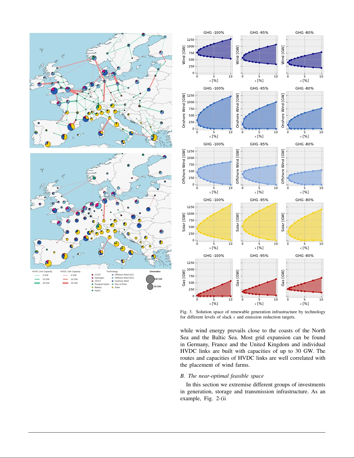
The Near -Optimal Feasible Space of a Rene w able Po wer System Model Fabian Neumann T om Brown Institute for Automation and Applied Informatics Karlsruhe Institute of T echnology (KIT) Karlsruhe, Germany { fabian.neumann, tom.brown } @kit.edu Abstract —Models for long-term in vestment planning of the power system typically return a single optimal solution per set of cost assumptions. However , typically there are many near -optimal alternatives that stand out due to other attractive properties like social acceptance. Understanding features that persist across many cost-efficient alternativ es enhances policy advice and acknowledges structural model uncertainties. W e apply the modeling-to-generate-alternatives (MGA) methodol- ogy to systematically explore the near-optimal feasible space of a completely renewable European electricity system model. While accounting for complex spatio-temporal patterns, we allow simultaneous capacity expansion of generation, storage and transmission infrastructure subject to linearized multi-period optimal power flow . Many similarly costly , but technologically diverse solutions exist. Already a cost deviation of 0.5% offers a large range of possible in vestments. Howev er , either offshore or onshore wind energy along with some hydr ogen storage and transmission network reinfor cement appear essential to keep costs within 10% of the optimum. Index T erms —power system modeling, power system eco- nomics, optimization, sensitivity analysis, modeling to generate alternativ es I . I N T RO D U C T I O N As governments across the world are planning to increase the share of rene wables, energy system modeling has become a pivotal instrument for finding cost-efficient future energy system layouts. Energy system models formulate a cost mini- mization problem and typically return a single optimal solution per set of input parameters (e.g. cost assumptions). Howe ver , feasible but sub-optimal solutions may be prefer- able for reasons that are not captured by model formulations because they are difficult to quantify [1]. Public acceptance of large infrastructure projects, such as many onshore wind turbines or transmission network expansion, ease of imple- mentation, land-use conflicts, and regional inequality in terms of po wer supply are prime examples of considerations which are exogenous to most energy system models. Bypassing such issues to enable a swift decarbonization of the ener gy system may justify a limited cost increase. F .N. and T .B. gratefully acknowledge funding from the Helmholtz Association under grant no. VH-NG-1352. The responsibility for the contents lies with the authors. Thus, providing just a singular optimal solution per scenario underplays the degree of freedom in designing cost-efficient future energy systems. Instead, presenting multiple alternativ e solutions and pointing out features that persist across many near-optimal solutions can remedy the lack of certainty in energy system models [2], [3]. Communicating model results as a set of alternati ves helps to identify must-haves (in vestment decisions common to all near-optimal solutions) and must- avoids (inv estment decisions not part of any near-optimal solution) [4]. The resulting boundary conditions can then inform political debate and support consensus building. A common technique for determining multiple near-optimal solutions is called Modeling to Generate Alternativ es (MGA) which uses the optimal solution as an anchor point to explore the surrounding decision space for maximally dif ferent solu- tions [1]. Other methods, such as scenario analysis, global sensitivity analysis, Monte Carlo analysis and stochastic pro- graming, that like wise address uncertainty in energy system modeling, concern parametric uncertainty , i.e. how inv estment choices change as cost assumptions are varied [3], [5], [6], [7]. Con versely , MGA explores inv estment flexibility for a single set of input parameters, by which it accounts for structural uncertainty and simplifications of model equations. In consequence, MGA is a complement rather than a substitute for methods sweeping across the parameter space. Evidence from previous work suggests many technologi- cally div erse solutions exist that result in similar total system costs for a sustainable European power system [15], [16]. These two studies research the sensitivity of cost input pa- rameters or the rele vance of transmission network expansion for low-cost power system layouts considering 30 regions. Previous studies that applied MGA to long-term ener gy sys- tem planning problems or retrospective analyses are revie wed in T able I. This work is the first to apply MGA to a European pan-continental electricity system model which includes an adequate number of regions and operating conditions to reflect the complex spatio-temporal patterns shaping cost-efficient in vestment strate gies in a fully rene wable system. Furthermore, the co-optimization of generation, storage and transmission infrastructure subject to linear optimal power flow (LOPF) constraints is unique for MGA applications. The goal of this work is to systematically explore the wide Accepted at 21st Power Systems Computation Conference Porto, Portugal — June 29 – July 3, 2020 T ABLE I L I TE R A T U R E R E VI E W : S T UD I E S A P PLY I NG M G A T O E N E R GY S Y ST E M M O D E LS Main Max. GHG MGA Cost Near-optimal Source Sector Region Nodes Snapshots Pathw ay Reduction Objectiv e Deviation Solutions LOPF Price et al. [8] coupled (IAM) global 16 > 1 yes 50% energy < 10% 30 no DeCarolis et al. [9] electricity US 1 1 no 85% capacity < 25% 9 no DeCarolis et al. [1] electricity US 1 1 yes 80% energy < 10% 28 no Li et al. [10] electricity UK 1 > 1 yes 80% any < 15% 800 no Sasse et al. [11] electricity CH 2,258 1 no none energy < 20% 2,000 no T rutnevyte et al. [12] electricity UK 1 3 no none any < 23% 250,500 no Berntsen et al. [13] electricity CH 1 386 no none any N/A 520 no Nacken et al. [14] coupled DE 1 8,760 no 95% capacity < 10% 1,025 no Hennen et al. [4] urban energy generic 1 > 1 no none capacity < 10% 384 no This study electricity Europe 100 4,380 no 100% capacity < 10% 1,968 yes IAM–Inte grated Assessment Model, GHG–gr eenhouse-gas, MGA–Modeling to Gener ate Alternatives, LOPF–Linear Optimal P ower Flow , UK–United Kingdom, CH–Switzerland, US–United States of America, DE–Germany array of similarly costly but div erse technology mixes for the European po wer system, and deri ve a set of rules that must be satisfied to k eep costs within pre-defined ranges. Additionally , we inv estigate how the e xtent of in vestment flexibility changes as we apply more ambitious greenhouse gas (GHG) emission reduction tar gets up to a complete decarbonization and allow varying levels of relative cost increases. The remainder of the paper is structured as follows: Section II guides through the problem formulation, the employed v ari- ant of MGA, sources of model input data, and the experimental setup. The results are presented and discussed from dif ferent perspectiv es in Section III and critically appraised in Section IV. The work is concluded in Section V. I I . M E T H O D O L O G Y A. Pr oblem formulation for long-term power system planning The objectiv e of long-term power system planning is to minimize the total annual system costs, comprising annu- alised 1 capital costs c ∗ for in vestments at locations i in generator capacity G i,r of technology r , storage capacity H i,s of technology s , and transmission line capacities F ` , as well as the variable operating costs o ∗ for generator dispatch g i,r,t : min G,H,F ,g f ( G, H, F , g ) = min G,H,F ,g   X i,r c i,r · G i,r + X i,s c i,s · H i,s + X ` c ` · F ` + X i,r,t w t · o i,r · g i,r,t   (1) where representative snapshots t are weighted by w t such that their total duration adds up to one year; P T t =1 w t = 365 · 24 h = 8760 h. The objective function is sub- ject to a set of linear constraints, including multi-period linear optimal po wer flow (LOPF) equations, resulting in a con vex linear program (LP). 1 The annuity factor 1 − (1+ τ ) − n τ con verts the overnight inv estment of an asset to annual payments considering its lifetime n and cost of capital τ . The capacities of generation, storage and transmission in- frastructure are constrained by their geographical potentials: G i,r ≤ G i,r ≤ G i,r ∀ i, r (2) H i,s ≤ H i,s ≤ H i,s ∀ i, s (3) F ` ≤ F ` ≤ F ` ∀ ` (4) The dispatch of a generator may not only be constrained by its rated capacity but also by the av ailability of variable renew able ener gy , which may be deri ved from reanalysis weather data. This can be expressed as a time- and location- dependent availability factor g i,r,t , given in per-unit of the generator’ s capacity: 0 ≤ g i,r,t ≤ g i,r,t G i,r ∀ i, r , t (5) The dispatch of storage units is split into two positiv e variables; one each for charging h + i,s,t and discharging h − i,s,t . Both are limited by the power rating H i,s of the storage units. 0 ≤ h + i,s,t ≤ H i,s ∀ i, s, t (6) 0 ≤ h − i,s,t ≤ H i,s ∀ i, s, t (7) This formulation does not prevent simultaneous charging and discharging, in order to maintain the computational benefit of a con vex feasible space. The energy le vels e i,s,t of all storage units have to be consistent with the dispatch in all hours. e i,s,t = η w t i,s, 0 · e i,s,t − 1 + w t · h inflow i,s,t − w t · h spillage i,s,t ∀ i, s, t + η i,s, + · w t · h + i,s,t − η − 1 i,s, − · w t · h − i,s,t (8) Storage units can have a standing loss η i,s, 0 , a charging efficienc y η i,s, + , a dischar ging ef ficiency η i,s, − , natural inflo w h inflow i,s,t and spillage h spillage i,s,t . The storage energy lev els are assumed to be cyclic e i,s, 0 = e i,s,T ∀ i, s (9) and are constrained by their energy capacity 0 ≤ e i,s,t ≤ T s · H i,s ∀ i, s, t. (10) T o reduce the number of decisison v ariables, we tie the energy storage volume to power ratings using a technology-specific parameter T s that describes the maximum duration a storage unit can discharge at full power rating. Accepted at 21st Power Systems Computation Conference Porto, Portugal — June 29 – July 3, 2020 Kirchhoff ’ s Current Law (KCL) requires local generators and storage units as well as incoming or outgoing flo ws f `,t of incident transmission lines ` to balance the inelastic electricity demand d i,t at each location i and snapshot t X r g i,r,t + X s h i,s,t + X ` K i` f `,t = d i,t ∀ i, t (11) where K i` is the incidence matrix of the network. Kichhoff ’ s V oltage Law (KVL) imposes further constraints on the flow of passiv e A C lines. Using linearized load flow assumptions, the voltage angle difference around e very closed cycle in the network must add up to zero. This constrained can be formulated using a cycle basis of the network graph where the independent cycles c that span the cycle space are expressed as directed linear combinations of lines ` in a cycle incidence matrix C `c [17]. This leads to the constraint X ` C `c · x ` · f `,t = 0 ∀ c, t (12) where x ` is the series inducti ve reactance of line ` . The controllable HVDC links are not affected by this constraint. All line flows f `,t are also limited by their capacities F ` | f `,t | ≤ f ` F ` ∀ `, t, (13) where f ` acts as a per -unit security mar gin on the line capacity . Finally , total CO 2 emissions may not exceed a target le vel Γ CO 2 . The emissions are determined from the time-weighted generator dispatch w t · g i,r,t using the specific emissions ρ r of fuel r and the generator efficiencies η i,r : X i,r,t ρ r · η − 1 i,r · w t · g i,r,t ≤ Γ CO 2 . (14) Note, that this formulation does not include pathway opti- mization (i.e. no sequences of inv estments), but searches for a cost-optimal layout corresponding to a gi ven GHG emission reduction lev el. For capacity expansion planning, it assumes perfect foresight for the reference year based on which capac- ities are optimized. Additional aspects such as reserve power , system stability , or robust scheduling hav e not been considered here. The optimization problem is implemented in the open- source modeling framew ork PyPSA [18]. B. Modeling to generate alternatives (MGA) As shown in Fig. 1, following a run of the original model, the objective function is encoded as a constraint such that the original feasible space is limited by the optimal objecti ve v alue f ∗ plus some acceptable relative cost increase  . f ( G, H , F, g ) ≤ (1 +  ) · f ∗ (15) Other than preceding studies, this paper pursues a more structured approach to MGA to span the near-optimal fea- sible space. The search directions are not determined by the Hop-Skip-Jump (HSJ) algorithm that seeks to minimize the weighted sum of v ariables of previous solutions [5], but by pre-defined groups of inv estment variables. Consequently , the new objective function becomes to variously minimize 0.0 0.1 0.2 0.3 0.4 0.5 0.6 0.7 0.8 0.9 x 1 0.0 0.1 0.2 0.3 0.4 0.5 0.6 0.7 0.8 x 2 feasible space I s o l i n e f ( x ) = f ( x * ) I s o l i n e f ( x ) = ( 1 + ) f ( x * ) O p t i m u m x * = a r g m i n x f ( x ) m i n { x 1 : f ( x ) ( 1 + ) f ( x * ) } m a x { x 1 : f ( x ) ( 1 + ) f ( x * ) } Fig. 1. Illustration of the near-optimal feasible space and the modeling to generate alternatives (MGA) methodology for a two-dimensional problem for the search-directions relating to dimension x 1 . and maximize sums of subsets of generation, storage and transmission capacity expansion variables giv en the  -cost constraint. The groups can be formed by region and by technology . Examples for thought-prov oking search directions are to min- imize the sum of onshore wind capacity in Germany or the total volume of transmission expansion (cf. Section II-D). This process yields boundaries within which all near- optimal solutions are contained and can be interpreted as a set of rules that must be followed to become nearly cost-optimal. In fact, by arguments of con ve xity , it can be sho wn that near - optimal solutions exist for all values of a group’ s total capacity between their corresponding minima and maxima. The original problem is con vex as it classifies as a linear program. Neither adding the linear  -cost constraint nor introducing an auxiliary variable z that represents the sum of the group of variables alter this characteristic. Hence, for any total z ∈ [ z min , z max ] a near-optimal solution e xists, howe ver not for any combination of its composites leading to this total. C. Model input data The exploration of the near-optimal feasible space is exe- cuted for the open model dataset PyPSA-Eur of the European power system with a spatial resolution of 100 nodes and a temporal resolution of 4380 snapshots (two-hourly for a full year) [23]. The chosen le vels of geographical and temporal aggregation reflect, at the upper end, the computational limits to calculate a large ensemble of near-optimal solutions and, at the lower end, the minimal requirements to expose trans- mission bottlenecks and account for spatially and temporally varying renewable potentials with passable detail [24], [25]. Follo wing a greenfield approach (with the exception of the transmission grid and hydropower installations), we allow simultaneous capacity expansion of transmission lines, HVDC links and v arious types of storage units and generators: solar photov oltaics, onshore wind turbines, offshore wind turbines with A C or DC grid connections, battery storage, hydrogen storage and, ultimately , open- and combined c ycle gas turbines (OCGT/CCGT) as sole fossil-fueled plants. Run-of-riv er and pumped-hydro capacities are not extend- able due to assumed geographical constraints. All other gener - ators and storage units can be built at any location up to their Accepted at 21st Power Systems Computation Conference Porto, Portugal — June 29 – July 3, 2020 T ABLE II A S SU M P T IO N S F O R T E C HN O - E CO N O M IC I N PU T P A R A M ET E R S T echnology e In vestment Fixed O&M Marginal Lifetime Efficiency In vestment T f Source [ e /kW] [ e /kW/a] [ e /MWh] [a] [-] [ e /kWh] [h] Onshore W ind 1330 33 2.3 25 1 DEA [19] Offshore Wind (A C) 1890 44 2.7 25 1 DEA [19] Offshore Wind (DC) 2040 47 2.7 25 1 DEA [19] Solar 600 25 0.01 25 1 Schrder et al. [20] Run of Riv er 3000 60 0 80 0.9 Schrder et al. [20] OCGT a 400 15 58.4 b 30 0.39 Schrder et al. [20] CCGT a 800 20 47.2 b 30 0.5 Schrder et al. [20] Hydrogen 689 24 0 20 0.8 · 0.58 c 8.4 168 Budischak et al. [21] Battery 310 9 0 20 0.81 · 0.81 c 144.6 6 Budischak et al. [21] Pumped Hydro 2000 20 0 80 0.75 N/A d 6 Schrder et al. [20] Hydro Reserv oir 2000 20 0 80 0.9 N/A d fixed Schrder et al. [20] T ransmission (submarine) 2000 e /MWkm 2% 0 40 1 Hagspiel et al. [22] T ransmission (ov erhead) 400 e /MWkm 2% 0 40 1 Hagspiel et al. [22] a Gas turbines have a CO 2 emission intensity of 0.19 t/MW th . b This includes fuel costs of 21.6 e /MWh th . c The storage round-trip ef ficiency consists of char ging and discharging ef ficiencies η + · η − . d The installed facilities are not e xpanded in this model and are considered to be amortized. e For all technologies a discount rate of 4% is assumed. f This relates a storage unit’ s energy capacity to its po wer capacity; it is the maximum duration the storage unit can discharge at full po wer capacity . geographical potentials. The corridors for ne w HVDC links, limited to 30 GW , are taken from the TYNDP 2018 [26]. Individual A C transmission line capacities may be expanded continuously up to four times their current capacity , but not reduced. W e further assume that the annual electricity demand for the po wer sector does not deviate substantially from today’ s lev els. Given the densely meshed and spatially aggregated transmission system, we do not add ne w expansion corridors but constrain options to reinforcement via parallel A C lines. T o approximate N − 1 security , the effecti ve transfer capacity of transmission lines is restricted to 70% of their nominal rating [23]. The dependence of line capacity expansion on line impedance is addressed in a sequential linear programing approach [27]. This relaxation is justified as it remov es the excessi ve computational burden of inte ger programming, while yielding equally accurate solutions given tolerated optimality gaps in discrete problems and other more decisiv e model condensations (e.g. network clustering) [27]. Full details on the workflow of PyPSA-Eur and processing the underlying datasets can be found in [23]. Cost assumptions and further techno-economic input parameters are listed in T able II. D. Experimental setup The MGA analysis is run within a par- allelized w orkflow for different de viations  ∈ { 0.5%, 1%, 2%, 3%, 4%, 5%, 7.5%, 10% } from the cost-optimal solution and for system-wide greenhouse-gas emission reduction targets of 80%, 95% and 100% compared to emission lev els in 1990. This allows to follo w the propagation of in vestment flexibility for increasing optimality tolerances and more ambitious climate protection plans. The alternativ e objecti ves are to minimize and maximize the generation capacity of all (i) wind turbines, (ii) onshore wind turbines, (iii) offshore wind turbines, (iv) solar panels, and (v) natural gas turbines. Moreover , we search for the minimal and maximal deployment of (vi) hydrogen storage, (vii) T ABLE III S T AT IS T I CS O N O P T I MA L S O L U TI O N S F O R D I FFE R E N T G H G E M I S SI O N R E DU C T I ON L E VE L S GHG Emissions -100% -95% -80% Generation [TWh] Onshore W ind 750 (24%) 421 (14%) 423 (15%) Offshore Wind (A C) 886 (28%) 568 (19%) 297 (10%) Offshore Wind (DC) 873 (27%) 1032 (34%) 769 (27%) Solar 502 (16%) 605 (20%) 381 (13%) Run of Riv er 150 (5%) 153 (6%) 154 (5%) CCGT (g as) 0 (0%) 171 (6%) 761 (26%) OCGT (g as) 0 (0%) 41 (1%) 105 (4%) T ransmission [TWkm] 504 (+71%) 458 (+55%) 368 (+25%) Load [TWh] 3,138 3,138 3,138 T otal Cost [bn e /a] 246 207 165 T otal Cost [ e /MWh] 78.4 66.1 52.6 battery storage, and (viii) power transmission infrastructure. This setup yields 384 near-optimal solutions. On av erage, each problem required 6.5 hours and 31 GB of memory to solve with the Gurobi solver . For slacks  ∈ { 1%, 5%, 10% } and a 95% emission reduc- tion tar get a 3-hourly resolved model is run for country-wise minima and maxima of the in vestment groups above, resulting in additional 1584 near-optimal solutions. On average, each problem required 3.5 hours and 22 GB of memory to solve. I I I . R E S U L T S A N D D I S C U S S I O N A. Optimal solutions Before delving into near -optimal solutions, we first outline the characteristics of the optimal solutions for dif ferent emis- sion reduction lev els (cf. T able III). A system optimized for a 100% emission reduction is strongly dominated by wind energy . More than half of the electricity is supplied by of fshore wind installations. Onshore wind turbines provide another quarter . In contrast, photov oltaics account for only 16% of electricity generation. Strikingly , a system targeting a 95% reduction in greenhouse gases uses significantly less onshore wind generators but more solar energy in comparison to a Accepted at 21st Power Systems Computation Conference Porto, Portugal — June 29 – July 3, 2020 (i) Optimal Transmission Network Expansion:  = 0% / GHG -100% HVAC Line Capacity 5 GW 10 GW 20 GW HVDC Link Capacity 5 GW 10 GW 20 GW Technology CCGT Hydrogen OCGT Pumped Hydro Battery Hydro Offshore Wind (AC) Offshore Wind (DC) Onshore Wind Run of River Solar Generation 100 GW 50 GW 10 GW Generation 100 GW 50 GW 10 GW (ii) Minimize Transmission Network Expansion:  = 10% / GHG -100% HVAC Line Capacity 5 GW 10 GW 20 GW HVDC Link Capacity 5 GW 10 GW 20 GW Technology CCGT Hydrogen OCGT Pumped Hydro Battery Hydro Offshore Wind (AC) Offshore Wind (DC) Onshore Wind Run of River Solar Generation 100 GW 50 GW 10 GW Generation 100 GW 50 GW 10 GW Fig. 2. Maps of transmission line expansion and regional generator and storage capacities for a 100% renewable power system for the (i) optimal solution and (ii) minimal transmission v olume within a 10% cost increase. completely decarbonized system, while keeping the share of offshore wind generation constant. Thus, for the last mile from 95% to 100% more onshore wind generation is preferred to phase out the last remaining natural-gas-fired power plants. The total system costs scale non-linearly with more tight emission caps. Achieving an emission reduction of 95% is roughly a quarter more expensi ve than a reduction by 80%, while a zero-emission system is almost 50% more expensi ve. Also, the map in Fig. 2-(i) shows the optimal regional distribution of the capacities of power system components for a fully renewable European power system. Generation hubs tend to form along the coasts of North, Baltic and Mediter- ranean Sea, whereas inland regions produce little electricity . Expectedly , solar energy is the dominant carrier in the South, 0 5 10 ² [ % ] 0 250 500 750 1000 1250 Wind [GW] GHG -100% 0 5 10 ² [ % ] Wind [GW] GHG -95% 0 5 10 ² [ % ] Wind [GW] GHG -80% 0 5 10 ² [ % ] 0 250 500 750 1000 1250 Onshore Wind [GW] GHG -100% 0 5 10 ² [ % ] Onshore Wind [GW] GHG -95% 0 5 10 ² [ % ] Onshore Wind [GW] GHG -80% 0 5 10 ² [ % ] 0 250 500 750 1000 1250 Offshore Wind [GW] GHG -100% 0 5 10 ² [ % ] Offshore Wind [GW] GHG -95% 0 5 10 ² [ % ] Offshore Wind [GW] GHG -80% 0 5 10 ² [ % ] 0 250 500 750 1000 1250 Solar [GW] GHG -100% 0 5 10 ² [ % ] Solar [GW] GHG -95% 0 5 10 ² [ % ] Solar [GW] GHG -80% 0 5 10 ² [ % ] 0 250 500 750 1000 1250 Gas [GW] GHG -100% 0 5 10 ² [ % ] Gas [GW] GHG -95% 0 5 10 ² [ % ] Gas [GW] GHG -80% Fig. 3. Solution space of renewable generation infrastructure by technology for dif ferent le vels of slack  and emission reduction targets. while wind energy pre vails close to the coasts of the North Sea and the Baltic Sea. Most grid expansion can be found in Germany , France and the United Kingdom and indi vidual HVDC links are built with capacities of up to 30 GW . The routes and capacities of HVDC links are well correlated with the placement of wind farms. B. The near-optimal feasible space In this section we extremise dif ferent groups of in vestments in generation, storage and transmission infrastructure. As an example, Fig. 2-(ii) depicts a system that seeks to deviate from the optimum by minimizing the volume of transmission network expansion up to a total cost increase of 10%, for Accepted at 21st Power Systems Computation Conference Porto, Portugal — June 29 – July 3, 2020 instance as a concession to better social acceptance. With the results particularly the NordSued link connecting Northern and Southern Germany manifests as a no-regret in vestment decision up to a capacity of 15 GW in the context of full decarbonization. It is one of the few persistent expansion routes. All other transmission e xpansion corridors are (to a significant extent) not compulsory . Missing transmission capacities can be compensated by adding storage capacity and more regionally dispersed po wer generation. Nevertheless, some transmission network reinforcement is indispensable to remain within the given cost bounds. These results are also broadly aligned with findings in [15], [24]. Beyond this example, the MGA results offer insights about the structure of the near-optimal space. The intent is to portray a set of technology-specific rules that must be satisfied to keep costs within pre-defined ranges  . Note, that the discontinuity created by  restricts the accuracy of the solution space. Fig. 3 rev eals that wind generation, either onshore or offshore, is essential to set up a cost-efficient European po wer system for all three e valuated emission reduction le vels. Whilst already a small cost increase of 0.5% yields in vestment flexibilities in the range of ± 100 GW , e ven a 10% more costly solution would still require more than 500 GW of wind generation capacity for a fully renew able system: tw o-thirds of the optimal system layout. Howe ver , even for a zero-emission system a cost increase of just 4% enables abstaining from onshore wind po wer, and a 7.5% more expensi ve alternati ve can function without offshore wind farms. The in vestment flexibility dev elops non-linearly with in- creasing slack lev els  . Even a minor deviation from the cost optimum by 0.5% creates room for maneuver in the range of ± 200 GW for onshore and ± 150 GW offshore wind installations, which indicates a weak tradeoff between onshore and offshore wind capacities very close to the optimum. Nonetheless, dispensing with both is not viable. Furthermore, 10% of total system costs must be spent to rule out solar panels, b ut already a slack of 1% allows to reduce the solar capacity by a third. Price et al. observed in their model that inv estment flexibil- ity in generation infrastructure decreased as more tight caps on carbon-dioxide emissions were imposed [8]. While it is true that more ambitions climate protection plans incur more must-hav es (i.e. minimum requirements of capacity), for the case-study at hand the viable ranges of marginally inferior solutions increase as more total capacity is built. As Fig. 4 exhibits, even for a complete decarbonization of the European po wer system building battery storage is not essential, although they are deployed in response to e.g. minimizing netw ork reinforcement. Con v ersely , once weather- independent dispatch flexibility from natural-gas-fired power plants is una vailable, it becomes imperativ e to counter-balance with hydrogen storage. The cutback of hydrogen infrastructure under these circumstances goes along with building excess generation capacities and multiplied amounts of curtailment. The reinforcement of the transmission network becomes more pi votal the more the power system is based on rene w- 0 5 10 ² [ % ] 0 250 500 750 1000 1250 Storage [GW] GHG -100% 0 5 10 ² [ % ] Storage [GW] GHG -95% 0 5 10 ² [ % ] Storage [GW] GHG -80% 0 5 10 ² [ % ] 0 250 500 750 1000 1250 Hydrogen [GW] GHG -100% 0 5 10 ² [ % ] Hydrogen [GW] GHG -95% 0 5 10 ² [ % ] Hydrogen [GW] GHG -80% 0 5 10 ² [ % ] 0 250 500 750 1000 1250 Battery [GW] GHG -100% 0 5 10 ² [ % ] Battery [GW] GHG -95% 0 5 10 ² [ % ] Battery [GW] GHG -80% 0 5 10 ² [ % ] 0 250 500 750 1000 1250 Transmission [TWkm] GHG -100% today's grid 0 5 10 ² [ % ] Transmission [TWkm] GHG -95% today's grid 0 5 10 ² [ % ] Transmission [TWkm] GHG -80% today's grid Fig. 4. Solution space of storage and transmission infrastructure by technol- ogy for different levels of slack  and emission reduction targets. ables. Aiming for an emission reduction by 80% a 2% more expensi ve v ariant can get by without any grid reinforcement. Reducing emissions by 100% still requires some additional power transmission capacity at a 10% cost de viation. Ho wever , within this range, the transmission volume can deviate from almost double of today’ s network capacities to merely a marginal reinforcement (cf. Fig. 2). MGA iterations were also applied from a country-wise perspectiv e. Remarkably , any one country could completely forego any one generation or storage technology and remain within 5% of the cost optimum when targeting a 95% reduc- tion in greenhouse gas emissions. In this case, neighboring countries must offset the absence of this technology . C. Corr elations So far , the study of the near-optimal feasible space did not capture the interdependence between different system components apart from the en velopes the analysis pro vided for each technology . Shifting to the extremes of one technology will diminish the inv estment flexibility of other carriers. Fig. 5 demonstrates ho w div ersity in capacity mixes rises if more Accepted at 21st Power Systems Computation Conference Porto, Portugal — June 29 – July 3, 2020 0 500 1000 1500 2000 - MIN - GW ² : 1 . 0 % ² : 5 . 0 % ² : 1 0 . 0 % Wind Onshore Wind Offshore Wind Solar Battery Hydrogen Storage Transmission 0 500 1000 1500 2000 - MAX - GW ² : 1 . 0 % Wind Onshore Wind Offshore Wind Solar Battery Hydrogen Storage Transmission ² : 5 . 0 % Wind Onshore Wind Offshore Wind Solar Battery Hydrogen Storage Transmission ² : 1 0 . 0 % Technology Hydrogen Pumped Hydro Battery Hydro Solar Run of River Onshore Wind Offshore Wind (DC) Offshore Wind (AC) OCGT CCGT Technology Hydrogen Pumped Hydro Battery Hydro Solar Run of River Onshore Wind Offshore Wind (DC) Offshore Wind (AC) OCGT CCGT Fig. 5. Composition of generation and storage capacities for various near- optimal solutions with 100% renew ables. Each subplot corresponds to a slack lev el  and an optimization sense. The labels of the bar charts indicate which group of in vestment v ariables is included in the objectiv e. CCGT OCGT Offshore Wind (AC) Offshore Wind (DC) Onshore Wind Solar Hydrogen Battery Transmission CCGT OCGT Offshore Wind (AC) Offshore Wind (DC) Onshore Wind Solar Hydrogen Battery Transmission Capacity 0.8 0.4 0.0 0.4 0.8 Fig. 6. Correlations of capacities across all near-optimal solutions. leew ay is given in terms of system costs. The striking variety in capacity totals is largely attributable to the lower capacity factors of solar compared to wind ener gy . Hennen et al. suggested to present the intertwining of technologies through Pearson’ s correlation coef ficient across all near-optimal solutions [4]. Fig. 6 confirms many of the previously noted connections. Hydrogen storage substitutes natural gas turbines and is positiv ely correlated with onshore and offshore wind capacity , while battery deployment rather matches with solar installations. Likewise, transmission ex- pansion occurs in unison with onshore and offshore wind deployment. Thereby , hydrogen storage and transmission be- come complements for high renewable energy scenarios. W ith caution should be noted that CCGT and OCGT as well as A C- and DC-connected offshore wind installations have high correlations because they are grouped in the MGA iterations. 0.0 0.2 0.4 0.6 0.8 1.0 Cumulative Share of Electrictiy Demand 0.0 0.2 0.4 0.6 0.8 1.0 Cumulative Share of Electrictiy Generation GHG -100% GHG -95% GHG -80% Fig. 7. Lorenz curves for the optimal solutions at different emission reduction lev els relating the cumulativ e share of electricity generation to the cumulativ e share of demand in the 100 regions of the European power system model. 0.2 0.4 0.6 0.8 Gini [-] 400 600 800 TWkm transmission - storage - GHG -100% 0.2 0.4 0.6 0.8 Gini [-] transmission - - storage GHG -95% 0.2 0.4 0.6 0.8 Gini [-] - transmission - storage GHG -80% today's grid optimum 2 4 6 8 10 ² [ % ] Fig. 8. Dev elopment equitable power generation measured by the Gini coefficient in relation to the capacity of the power transmission network measured in TWkm. The four plotted search directions are minimization and maximization of each, total transmission v olume and storage capacity . D. Distributional equity Surve ys suggest that an equal distribution of power supply is preferred among the population and may increase their willingness to participate in the energy system transformation process [28]. Sasse et al. and Drechsler et al. in vestigate the trade-offs between least-cost and re gionally equitable solutions in Switzerland and Germany by using concepts of the Lorenz curves and the Gini coefficients as equity measures [11], [28]. In the context of power , the Lorenz curve can relate the cumulativ e share of electricity generation of regions to their cumulativ e share of electricity demand as sho wn in Fig. 7. For more ambitious emission reduction tar gets, less equitable solutions are fav ored from a cost-perspectiv e, howe ver , they may not be in line with the public attitude. The Gini coefficient is the corresponding scalar measure of uniformity and is determined by multiplying the area between the Lorenz curve and the identity line by two. A Gini coefficient of 1 represents the most unequal distribution, while 0 corresponds to the situation where ev ery region produces, on average, as much electricity as they consume. Preceding studies have, in general, noted that the focus on wind power tends to be detrimental to a regionally balanced distribution of electricity generation [28], whereas photov oltaic power supply is a key factor for an ev en distribution of the power supply [11]. This observation is consistent with the results of the European power system at hand. But as we consider the transmission grid and energy storage options, we can further extend on these findings. In Fig. 8 we track Accepted at 21st Power Systems Computation Conference Porto, Portugal — June 29 – July 3, 2020 the equity of solutions in relation to the transmission network volume as we approach the boundaries of either technology category . Substantially more re gionally equitable solutions are attainable for a limited cost-increase when div erting attention away from transmission network expansion. Utilizing less en- ergy storage rather discourages equitable generation patterns; in the opposite direction, this is not the case for a zero- emission system. Note that the equity measures are only an observed side-ef fect and not the objecti ve of a particular search direction of the MGA method. There is no guarantee that no more equitable solutions exist within the near-optimal feasible space. I V . C R I T I C A L A P P R A I S A L This paper covers the electricity sector only . Bro wn et al. suggested that with an increasing coupling of energy sectors the benefit of the transmission system decreases [29]. It is not far -fetched, that the near-optimal feasible space, in general, might look very dif ferent with a tightened sectoral inte gration. W ithin the computational constraints, it is moreov er desir- able to further enhance the spatial and temporal resolution to better reflect curtailment caused by transmission bottlenecks and factor in extreme weather e vents [24]. This w ork further ne glects parametric uncertainty . Coupling this paper’ s variant of MGA with a parameter sweeping method (such as Monte Carlo simulation [10]) would allow to derive a more sophisticated version of Fig. 3 and 4 with fuzzy boundaries that represent the probability with which the respective capacities of system components are contained within the near-optimal feasible space. V . S U M M A RY A N D C O N C L U S I O N S This work sheds light on the flatness of the near-optimal feasible decision space of a power system model with Euro- pean scope for ambitious climate protection targets. An understanding of alternatives beyond the least-cost solutions is indispensable to dev elop rob ust, credible and comprehensible policy guidelines. Therefore, we deriv ed a set of technology-specific boundary conditions that must be satisfied to keep costs within pre-defined ranges using the modeling-to-generate-alternativ es methodology . These rules permit well-informed discussions around social constraints to the exploitation of renewable resources or the extent to which the power transmission network can be reinforced in discussions. Indeed, we observed high variance in the deployment of individual system components, ev en for a fully renew able system. Already a minor cost deviation of 0.5% offers a multitude of technologically div erse alternatives. It is possible to dispense with onshore wind for a cost increase of 4%, and to forego solar for 10%. Nev ertheless, either offshore or onshore wind energy plus at least some hydrogen storage and grid reinforcement are essential to keep costs within 10% of the optimum. S U P P L E M E N T A RY M A T E R I A L For supplementary material and reading the reader is re- ferred to the source code repository on Github (https://github . com/pypsa/pypsa- eur - mga) and the documentations of PyPSA (https://pypsa.readthedocs.io, [18]) and PyPSA-Eur (https:// pypsa- eur .readthedocs.io, [23]). R E F E R E N C E S [1] J. F . DeCarolis, S. Babaee, B. Li, and S. Kanungo, “Modelling to generate alternatives with an energy system optimization model, ” En- vir onmental Modelling and Softwar e , v ol. 79, pp. 300–310, 2016. [2] S. Pfenninger, A. Hawkes, and J. K eirstead, “Energy systems modeling for twenty-first century energy challenges, ” Renewable and Sustainable Ener gy Revie ws , vol. 33, pp. 74–86, 2014. [3] J. DeCarolis, H. Daly , P . Dodds, I. Keppo, F . Li, W . McDowall, S. Pye, N. Strachan, E. T rutnevyte, W . Usher , M. Winning, S. Y eh, and M. Zeyringer , “Formalizing best practice for energy system optimization modelling, ” Applied Ener gy , vol. 194, pp. 184–198, 2017. [4] M. Hennen, M. Lampe, P . V oll, and A. Bardow , “SPREAD Exploring the decision space in energy systems synthesis, ” Computers and Chem- ical Engineering , vol. 106, pp. 297–308, 2017. [5] X. Y ue, S. Pye, J. DeCarolis, F . G. Li, F . Rogan, and B. O. Gallachoir , “ A review of approaches to uncertainty assessment in energy system optimization models, ” Energy Strate gy Reviews , vol. 21, pp. 204–217, Aug. 2018. [6] S. Moret, V . C. Girons, M. Bierlaire, and F . Marchal, “Characterization of input uncertainties in strategic energy planning models, ” Applied Ener gy , vol. 202, pp. 597 – 617, 2017. [7] B. Shirizadeh, Q. Perrier , and P . Quirion, “How sensitiv e are optimal fully rene wable po wer systems to technology cost uncertainty?” F AERE - French Association of Environmental and Resource Economists, Policy Papers 2019.04, 2019. [Online]. A vailable: https://EconPapers.repec.or g/RePEc:fae:ppaper:2019.04 [8] J. Price and I. Keppo, “Modelling to generate alternatives: A technique to explore uncertainty in ener gy-environment-economy models, ” Applied Ener gy , vol. 195, pp. 356–369, 2017. [9] J. F . DeCarolis, “Using modeling to generate alternativ es (MGA) to expand our thinking on energy futures, ” Energy Economics , vol. 33, no. 2, pp. 145–152, 2011. [10] F . G. Li and E. Trutnevyte, “In vestment appraisal of cost-optimal and near-optimal pathways for the UK electricity sector transition to 2050, ” Applied Ener gy , vol. 189, pp. 89–109, 2017. [11] J.-P . Sasse and E. Trutnevyte, “Distributional trade-offs between re- gionally equitable and cost-efficient allocation of renewable electricity generation, ” Applied Ener gy , vol. 254, p. 113724, 2019. [12] E. Trutne vyte, “Does cost optimization approximate the real-world energy transition?” Ener gy , v ol. 106, pp. 182–193, 2016. [13] P . B. Berntsen and E. Trutne vyte, “Ensuring diversity of national energy scenarios: Bottom-up energy system model with Modeling to Generate Alternativ es, ” Ener gy , v ol. 126, pp. 886–898, May 2017. [14] L. Nacken, F . Krebs, T . Fischer , and C. Hoffmann, “Integrated rene wable energy systems for Germany A model-based exploration of the decision space, ” 16th International Conference on the Eur opean Ener gy Mark et , 2019. [15] D. P . Schlachtberger , T . Brown, S. Schramm, and M. Greiner , “The Benefits of Cooperation in a Highly Renewable European Electricity Network, ” Energy , v ol. 134, pp. 469–481, Sep. 2017, arXiv: 1704.05492. [16] D. P . Schlachtberger , T . Brown, M. Schfer , S. Schramm, and M. Greiner, “Cost optimal scenarios of a future highly renewable European electric- ity system: Exploring the influence of weather data, cost parameters and policy constraints, ” Energy , vol. 163, pp. 100–114, Nov . 2018, arXiv: 1803.09711. [17] J. Hrsch, H. Ronellenfitsch, D. Witthaut, and T . Brown, “Linear optimal power flow using cycle flows, ” Electric P ower Systems Researc h , vol. 158, pp. 126–135, 2018, arXiv: 1704.01881. [18] T . Brown, J. Hrsch, and D. Schlachtberger , “PyPSA: Python for Power System Analysis, ” Journal of Open Researc h Software , vol. 6, p. 4, Jan. 2018. [19] Danish Energy Agency (DEA). (2019) T echnology data. [On- line]. A vailable: https://ens.dk/en/our- services/projections- and- models/ technology- data Accepted at 21st Power Systems Computation Conference Porto, Portugal — June 29 – July 3, 2020 [20] A. Schrder, F . Kunz, J. Meiss, R. Mendelevitch, and C. von Hirschhausen, “Current and prospective costs of electricity generation until 2050, ” DIW Berlin, DIW Data Documentation 68, 2013. [Online]. A v ailable: http://hdl.handle.net/10419/80348 [21] C. Budischak, D. Sewell, H. Thomson, L. Mach, D. E. V eron, and W . Kempton, “Cost-minimized combinations of wind power , solar po wer and electrochemical storage, powering the grid up to 99.9% of the time, ” Journal of P ower Sour ces , v ol. 225, pp. 60 – 74, 2013. [22] S. Hagspiel, C. Jgemann, D. Lindenberger , T . Brown, S. Chere vatskiy , and E. T rster, “Cost-optimal power system e xtension under flow-based market coupling, ” Ener gy , v ol. 66, pp. 654 – 666, 2014. [23] J. Hrsch, F . Hofmann, D. Schlachtberger , and T . Brown, “PyPSA-Eur: An open optimisation model of the European transmission system, ” En- er gy Strate gy Re views , v ol. 22, pp. 207–215, 2018, arXiv: 1806.01613. [24] J. Hrsch and T . Brown, “The role of spatial scale in joint optimisations of generation and transmission for European highly renewable scenarios, ” 14th International Conference on the European Ener gy Market , 2017, arXiv: 1705.07617. [25] S. Pfenninger, “Dealing with multiple decades of hourly wind and pv time series in energy models: A comparison of methods to reduce time resolution and the planning implications of inter-annual variability , ” Applied Ener gy , vol. 197, pp. 1 – 13, 2017. [26] ENTSO-E. (2018) TYNDP: T en-Y ear Network Development Plan. [Online]. A vailable: https://tyndp.entsoe.eu/tyndp2018/ [27] F . Neumann and T . Brown, “Heuristics for T ransmission Expansion Planning in Low-Carbon Energy System Models, ” 16th International Confer ence on the Eur opean Energy Market , 2019, arXiv: 1907.10548. [28] M. Drechsler , J. Egerer, M. Lange, F . Masurowski, J. Meyerhoff, and M. Oehlmann, “Efficient and equitable spatial allocation of renewable power plants at the country scale, ” Natur e Ener gy , vol. 2, no. 9, p. 17124, Sep. 2017. [29] T . Brown, D. Schlachtber ger, A. Kies, S. Schramm, and M. Greiner, “Synergies of sector coupling and transmission extension in a cost- optimised, highly renewable European energy system, ” Energy , pp. 720– 739, 2018, arXiv: 1801.05290. Accepted at 21st Power Systems Computation Conference Porto, Portugal — June 29 – July 3, 2020