Microseismic events enhancement and detection in sensor arrays using autocorrelation based filtering

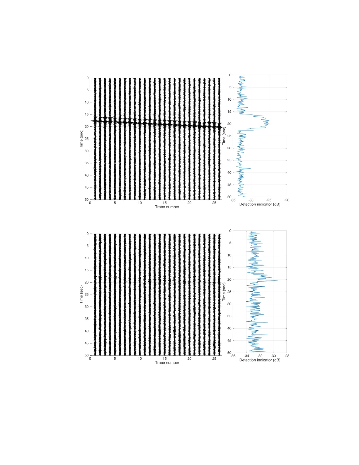
Microseismic ev en ts enhancemen t and detection in sensor arra ys using auto correlation based filtering En tao Liu ∗ 1 , Lijun Zh u 1 , An upama Go vinda Ra j 1 , James H. McClellan 1 , Abdullatif Al-Shuhail 2 , SanLinn I. Kak a 2 , and Nav eed Iqbal 2 1 CeGP at Georgia Institute of T ec hnology 2 CeGP at KFUPM Decem b er 7, 2016 Abstract P assive microseismic data are commonly buried in noise, whic h presents a significant c hallenge for signal detection and recov ery . F or recordings from a surface sensor arra y where each trace con tains a time-delay ed ar- riv al from the even t, w e prop ose an autocorrelation-based stacking metho d that designs a denoising filter from all the traces, as w ell as a multi-c hannel detection sc heme. This approac h circumv ents the issue of time aligning the traces prior to stacking b ecause every trace’s auto correlation is cen- tered at zero in the lag domain. The effect of white noise is concentrated near zero lag, so the filter design requires a predictable adjustment of the zero-lag v alue. T runcation of the auto correlation is emplo yed to smooth the impulse resp onse of the denoising filter. In order to extend the ap- plicabilit y of the algorithm, we also propose a noise prewhitening scheme that addresses cases with colored noise. The simplicit y and robustness of this metho d are v alidated with synthetic and real seismic traces. Keywor ds— passive seismic, denoising, detection, sensor array , auto corre- lation, filter design ∗ liuentao@gmail.com 1 1 In tro duction Microseismic monitoring is of great interest for its capability of providing v aluable information for many oil and gas related applications, such as hy- draulic fracturing monitoring, uncon ven tional reservoir characterization, and CO 2 sequestration (Duncan and Eisner 2010; Maxwell, White and F abriol 2004; Phillips et al. 2002; W arpinski 2009). In practice, microseismic monitoring is p erformed using downhole, surface, or near surface arra ys (Duncan and Eisner 2010). Recen tly , there is a preference for surface arrays which can be deplo yed more economically and efficiently . How ever, recorded surface microseismic sig- nals are muc h noisier than downhole data, b ecause surface or near surface arra ys are susceptible to b oth coherent and incoheren t noise. Consequen tly , it is challenging to extract useful information from the recorded microseismic data. Typically , the signal-to-noise ratio (SNR) of recorded micro- seismic data is rather low, esp ecially for the data collected using surface arrays. The noise adversely affects the accuracy of many microseismic analyses, such as P-w av e and S-wa ve arriv als picking, even t detection and localization, and fo cal mec hanism in version (Sabbione and V elis 2010; Zhang, Tian and W en 2014; Zh u, Liu and McClellan 2015). In fact, the ma jorit y of microseismic even ts induced by hydraulic fracturing has a typical moment magnitude M W < − 1 (Song et al. 2014). W e consider the case of a sensor arra y that records m ultiple traces, and as- sume that the microseismic signal of interest is present in all the traces. There- fore, stac king is one of the primary techniques to consider for improving SNR, as it is w ell known for seismic applications (Yilmaz 2001). How ever, for micro- seismic data time alignment of the traces, whic h is the prerequisite of stack- ing, is generally unkno wn. Th us, researchers ha ve developed algorithms based on cross-correlation to find the relativ e time delays b et ween traces (Al-Shuhail, Kak a and Jervis 2013; Grechk a and Zhao 2012). In contrast to the case of an ac- tiv e seismic where the source generates a con trollable activ e w a velet, the wa v elet of a microseismic even t is unkno wn, although some empirical kno wledge of the frequency domain characteristics may b e av ailable. The cross-correlations are usually computed from noisy traces rather than from a clean signal template. Therefore, the maximal v alue of the cross-correlation may occur at an incor- rect lag because of the noise. T o b ypass this b ottlenec k, we prop ose denoising and detection schemes using stac ked autocorrelograms, whic h are automatically aligned at the zero lag. The simplicity and robustness of the prop osed schemes are demonstrated by using b oth synthetic and real data. In the literature, the stac ked cross-correlation and auto correlation hav e already shown promising re- sults in different scenarios (Liu et al. 2016; W ap enaar et al. 2010a,b; Zhang et al. 2014). 2 2 Denoising Problem formulation Assume the sensor array for microseismic monitoring has N channels. Eac h recorded trace contains a microseismic wa veform contaminated by noise, i.e. x i ( t ) = a i s i ( t ) + n i ( t ) , i = 1 , . . . , N , (1) where a i are amplitude scaling factors, and n i ( t ) is zero mean additiv e white Gaussian noise (A W GN) with v ariance σ 2 . F or simplicit y , we first consider only white noise whose p o w er sp ectrum is flat; the colored noise scenario, whose p o w er densit y has differen t amplitudes for differen t frequencies, will be discussed in a later section. Theoretically , seismic traces received on differen t sensors are conv olutions of the same source w av elet with Green’s functions whic h are determined b y the real Earth and source and sensor lo cations (Aki and Ric hards 2009; Stein and Wysession 2002). Nonetheless, a high resemblance b et ween different traces originated by the same even t and collected by spatially close sensors is usually observ ed (Arrowsmith and Eisner 2006). Therefore, it is reasonable to assume that s i ( t ) are all the same wa v eform but with different time delays, i.e., s i ( t ) = s ( t − τ i ). In addition, w e assume the n i ( t ) are uncorrelated with the wa veform s ( t ) and independent of each other; uncorrelated noise on differen t c hannels is a common assumption for the v alidity of any stacking technique. The pro cessing is p erformed on digital signals, sampled at a rate f s = 1 / ∆ t , so that the time v ariable t b ecomes t l = t 0 + ( l − 1)∆ t for l = 1 , . . . , L . On each trace, w e consider a finite time window of data which contains L time samples, so the signals can be written as x i [ l ] = a i s i [ l ] + n i [ l ] , l = 1 , . . . , L (2) where x i [ l ] = x i ( t l ). In this work, we define the SNR of the i -th channel as the ratio of the signal energy to the A W GN energy , i.e., SNR i = 10 log 10  a 2 i k s i k 2 2 k n i k 2 2  . (3) As reference, we use the p eak-signal-to-noise ratio (PSNR) as w ell PSNR i = 10 log 10  a 2 i P 2 i σ 2  , (4) where P i is the p eak v alue of s i ( t ). When the w av elet duration is short, the PSNR is more in tuitive than SNR, because its v alue is not affected b y the signal length. 2.1 Denoising Filter Design The prop osed approach is implemented with the follo wing three steps: 3 1. Compute the auto correlation function (ACF) of eac h trace (denoted by ? ) and then stack the A CFs, r s [ τ ] = 1 N N X i =1 ( x i ? x i )[ τ ] , (5) where τ = − L + 1 , . . . , 0 , . . . , L − 1 is the lag index of the A CF. 2. Define the denoising filter’s impulse resp onse as a windo wed v ersion of the mo dified ACF, f [ τ ] = ˆ r s [ τ ] w d [ τ ], where ˆ r s [ τ ] =  1 2  r s [ − 1] + r s [1]  if τ = 0 r s [ τ ] otherwise (6) The zero-lag v alue of the ACF is replaced with the av erage of its neigh- b oring v alues, r s [1] and r s [ − 1]. The justification for this c hange is that additiv e white noise has an ACF that is Lσ 2 δ [ τ ], where δ [ τ ] is the discrete Dirac delta impulse function and only gives nonzero v alue at τ = 0. Thus the A CF r s [ τ ] has a large peak at τ = 0 which needs to b e reduced b y Lσ 2 ; the av erage of the neighboring v alues provides an estimate of the correct zero-lag v alue of the signal-only ACF. 3. A truncation window w d [ τ ] is then applied to the zero lag region, if nec- essary , so that the negligible v alues in the filter (aw ay from τ = 0) will b e eliminated. A prop er truncation window that shortens the filter length will impro ve the computational efficiency as well. V arious truncation windows are av ailable, how ever we adopt a simple triangle windo w w d [ τ ] = ( 1 − | τ | /d if | τ | ≤ d 0 otherwise (7) where 2 d + 1 is the length of the truncation window. 4. Con volv e f [ τ ] with each noisy trace in the collection. The result of these con volutions provides the N denoised traces ˆ x i [ l ] = ( f ∗ x i )[ l ] for i = 1 , 2 , . . . , N . In Figure 1, w e show the stack ed autocorrelation r s [ τ ] and the filter f [ τ ] based on it for the case of a 30-Hz Rick er wa velet sampled at f s = 500 Hz, whic h is also treated in the denoising example for synthetic data in Section 3.1. The spiky p eak in r s [ τ ] at zero lag is remo ved by the av erage op eration (6) to obtain f [ τ ]. Compared with a cross-correlation based metho d, this new auto correlation- based approach has approximately the same computational burden, since com- puting one ACF or one cross-correlation function (CCF) is O ( L log 2 ( L )). In fact, some ov erhead is remov ed b y av oiding the searc h for the maximal v alue needed for alignment. 4 -50 -25 0 25 50 Lag of points -5 0 5 10 15 20 25 Amplitude -50 -25 0 25 50 Lag of points -5 0 5 10 15 20 25 Amplitude (a) (b) Figure 1: (a) Stack ed auto correlation (b) denoising filter. L = 200 and σ = 0 . 3, so the p eak heigh t remov ed is approximately Lσ 2 = 18. 2.2 F requency Resp onse Analysis In order to ev aluate the p erformance of the designed filter, w e examine the frequency resp onse of the filter f [ τ ] since the analysis of the filter p erformance is easier to conduct in the frequency domain. The F ourier transform ( F ) of the A CF r s ( τ ) is R s ( e j ω ) = F { r s ( τ ) } = 1 N N X i =1 X i ( e j ω ) X i ( e j ω ) = 1 N N X i =1 ( a 2 i | S i ( e j ω ) | 2 + | N i ( e j ω ) | 2 + a i S i ( e j ω ) N i ( e j ω ) + a i N i ( e j ω ) S i ( e j ω )) ≈ | S ( e j ω ) | 2 1 N N X i =1 a 2 i + 1 N N X i =1 | N i ( e j ω ) | 2 , (8) where the last line is derived from the ass umption that the signal s ( t ) and noise n i ( t ) are uncorrelated. The t wo terms in (8) are scaled versions of the p o w er sp ectrum of the signal (i.e., magnitude squared), and the p o wer spectrum of the noise whic h is a random v ariable at each frequency ω . If we assume a i = 1 for all i , then there is no scaling of the first term. The second term is the exp ected v alue of the noise p o wer sp ectrum which for white noise is equal to Lσ 2 for all frequencies. W e can now justify the definition of ˆ r s [ τ ] in equation (6). Compared with the r s ( τ ), the designed filter is mo dified slightly from the auto correlation by remo ving the p eak at zero lag. How ev er, the frequency resp onse is beneficially manipulated for the denoising purp ose. F or ease of exp osition, we assume a i = 5 1 for all i . When the sampling frequency is high enough and noise is white f [0] = 1 2 ( r s [ − 1] + r s [1]) = r s [ − 1] turns out to be an accurate approximation of the energy of s ( t ). W e then can decomp ose r s [0] into tw o parts r s [0] = ˆ r s [0] + p. (9) Again, b ecause signal s ( t ) and noise n i ( t ) are uncorrelated, r s [0] = 1 N N X i =1 ( k x i k 2 2 ) = k s k 2 2 + 1 N N X i =1 k n i k 2 2 , (10) and ˆ r s [0] ≈ k s k 2 2 . (11) Subtracting equation (11) from (10), we obtain p ≈ 1 N N X i =1 k n i k 2 2 = 1 N L N X i =1 k N i ( e j ω ) k 2 2 , (12) b y Parsev al’s theorem. Therefore, p is approximately the av erage energy of the noise ov er all traces. W e reformulate r s [ τ ] as r s [ τ ] = ˆ r s [ τ ] + pδ [ τ ] . (13) F or a certain frequency ω , the frequency resp onse of the filter ˆ r s [ τ ] is exp ected to b e the pow er of the signal at ω when the noise is white, E [ F { ˆ r s [ τ ] } ] = E [ F { r s [ τ ] − pδ [ τ ] } ] = E [ F { r s [ τ ] } ] − p ≈ E [ 1 N N X i =1 | X i ( e j ω ) | 2 ] − 1 N L N X i =1 k N i ( e j ω ) k 2 2 ≈ E [ 1 N N X i =1 | S i ( e j ω ) | 2 ] + E [ 1 N N X i =1 | N i ( e j ω ) | 2 ] − 1 N L N X i =1 k N i ( e j ω ) k 2 2 ≈ E [ 1 N N X i =1 | S i ( e j ω ) | 2 ] . (14) Here we can see that the prop osed filter ˆ r s [ τ ] (without truncation) shifts the frequency resp onse amplitude of r s [ τ ] down b y p . The frequency resp onse of the filter is literally an estimation of the pow er sp ectrum of the signal. Due to the fo cal mec hanism of the seismic source, the w av eforms receiv ed on the sensor array can ha ve differen t amplitudes and phases (i.e., the signs of a i ). Corrections to the signs are helpful when we stac k the traces or p erform the cross correlations. Otherwise, stac king w a veforms of differen t signs would cancel 6 eac h other rather than enhance them. One adv antage of ACF-designed filter f [ τ ] ov er cross-correlation based metho d is that f [ τ ] is not affected by the signs of a i . Essentially , stac king autocorrelation is equiv alent to stac king squared frequency response amplitude in frequency domain where all a i are squared as in equation (8). The disp ersion of wa ve is another phenomenon whic h is harmful to the stacking techniques in the time domain. How ev er, the stack ed auto correlation is not affected by disp ersion, for the same reason. Although the idea of enhancing the signal in the frequency domain is widely used, one ob vious adv an tage of the prop osed scheme is that it pro duces a band pass filter (BPF) that adapts to the received signals instead of using a filter whose pass band is sp ecified a priori . Recall the truncation window in equation (7) applied to the filter, whic h ex- p edites the conv olution step. In addition, the truncation of the filter introduces a smo othing effect in its frequency resp onse. Usually , the smo othing effect is b eneficial to the denoising filter performance. 2.3 Noise whitening One of the basic assumptions b ehind the prop osed denoising scheme is that of additive white noise. In practice, seismic noise is often colored when it is related to the e n vironmen t, weather, or human activities. And hence the auto- correlation of the noise could b e far from an impulse function. So, we w ould not b e able to eliminate the noise’s frequency resp onse by manipulating the stack ed auto correlation v alue only at the zero lag p osition. T o generalize for the colored noise case, w e advocate a noise whitening sc heme based on linear prediction theory . Before discussing the whitening algorithm to flatten the noise sp ectrum, we state tw o assumptions: (1) the samples of the colored noise are from a stationary random pro cess, and (2) w e hav e a snapshot of the noise-only data of sufficient time duration. This second assumption would b e practical for microseismic monitoring, since the noise-only data can b e recorded b efore the fluid injection activities are started. Let v ( t ) b e the stationary , colored noise signal. An y wide sense stationary random pro cess can b e mo deled using an Auto Regressiv e (AR) mo del if the order of the model is c hosen large enough (Kay 1988; Makhoul 1975). Then w e can apply a linear prediction filter with co efficien ts { c k } to predict the next sample using P previous samples ˆ v [ l ] = P X k =1 c k v [ l − k ] , (15) where P is the order of the prediction filter. In general, the prediction is not p erfect, so there will b e a prediction error sequence e [ l ] = v [ l ] − ˆ v [ l ] . (16) 7 The optimal linear predictive co ding (LPC) co efficien ts minimizes the prediction error pow er of the P -th order linear predictor (Ka y 1988). This operation has b een shown equiv alen t to maximizing sp ectral flatness at the output of predic- tion error filter (Gray Jr. and Markel 1974; Markel and Gray Jr. 1976). F or an AR( P ) pro cess, the optimal prediction co efficien ts are the AR( P ) parameters itself. The prediction error filter thus acts as a whitening filter that decorrelates the input AR pro cess to pro duce white noise as its output. Determining P is the mo del order selection problem whic h can b e handled by using the fact for a linear predictor of order q , satisfying q > P where P is the true order of the AR pro cess, the error p o wer is constan t (Kay 1988). Ev en if the order of the AR( P ) pro cess and the order q selected for the linear predictor are not the same, the output prediction error will be white if q ≥ P . The blo c k diagram with the linear predictor used as a whitening filter is sho wn in Figure 2. In the z -transform domain the whitening filter H ( z ) is given b y H ( z ) = 1 − A ( z ) (17) where A ( z ) is the linear prediction filter A ( z ) = P X k =1 c k z − k . (18) The prediction co efficien ts c k can b e computed using the auto correlation metho d of AR mo deling. This inv olves estimating the auto correlation sequence from the time series and solving the Y ule-W alker equations through Levinson Durbin recursion (Kay 1988; Ljung 1987). The design of the whitening filter for eac h trace can be carried out during an initial noise-only segmen t of data. Then we whiten each noisy trace before designing the denoising filter f [ τ ]. d n fi lter .g r af fl e v [ l ] v [ l ] - + Error Sequence ˆ e [ l ] ˆ v [ l ] ˆ v [ l ] Figure 2: Whitening filter 3 Denoising examples 3.1 Syn thetic data: Ric k er wa v elet F or syn thetic data, we assume that there are 200 traces with identical am- plitude scaling, i.e., a i = 1. The wa veform s ( t ) is a Rick er w av elet with center frequency of 30 Hz and a normalized p eak v alue. The sampling frequency is 500 Hz and each trace has 200 time samples. Based on the SNR giv en in (3), t wo cases are considered: − 6 . 03 dB and − 12 . 01 dB, where the A WGN has σ = 0 . 3 8 and 0 . 6, resp ectiv ely . In Figure 3 w e sho w noiseless signals sup erimp osed on noisy versions for these t wo cases. Recall that plots of the stack ed ACFs shown previously in Figure 1 w ere generated for the case of σ = 0 . 3. Time (S) 0 0.05 0.1 0.15 0.2 0.25 0.3 0.35 0.4 Amplitdue -1.5 -1 -0.5 0 0.5 1 1.5 2 2.5 Noiseless signal Noisy trace Time (S) 0 0.05 0.1 0.15 0.2 0.25 0.3 0.35 0.4 Amplitdue -1.5 -1 -0.5 0 0.5 1 1.5 2 2.5 Noiseless signal Noisy trace (a) (b) Figure 3: Noiseless and noisy traces, (a) SNR= − 6 . 03 dB; (b) SNR= − 12 . 01 dB. The corresp onding PSNR v alues are 10 . 46 dB and 4 . 44 dB, resp ectiv ely . F or conciseness, we present only the first 20 noisy traces of these t wo noise lev els in Figures 4(a) and 4(c), resp ectiv ely . The final denoising results b y the prop osed scheme are shown in Figures 4(b) and 4(d). In b oth cases, the micro- seismic even ts in these v ery lo w SNR datasets are significantly enhanced. F or the low noise case, the denoised data ha ve SNR=2.51 dB (i.e., PSNR=17.60 dB). Additionally , the high noise case, the denoised data hav e SNR=0.51 dB (i.e., PSNR=10.84 dB). In order to track the in termediate steps of the sc heme, we compare the stac ked autocorrelation and the designed filter side b y side in Figure 1 for the lo w noise case. Then Figure 5 illustrates the filter with and without truncation for the σ = 0 . 3 and σ = 0 . 6 cases. The effect of smo othing in the frequency domain is then shown in Figure 6, which displa ys the frequency resp onses of the filters in Figure 5. 3.2 Field data In order to test the v alidity of the proposed sc heme with microseismic data that would b e receiv ed by a surface sensor array , we generate a set of 182 traces with different time dela ys from a single seismic trace. The wa v eform used in this study comes from the High Resolution Seismic Netw ork (HRSN) op erated b y Berkeley Seismological Lab oratory , Universit y of California, Berk eley , the Northern California Seismic Net work (NCSN) op erated by the U.S. Geological 9 Sensor Index 0 10 20 Time (s) 0 0.05 0.1 0.15 0.2 0.25 0.3 0.35 Sensor Index 0 10 20 Time (s) 0 0.05 0.1 0.15 0.2 0.25 0.3 0.35 Sensor Index 0 10 20 Time (s) 0 0.05 0.1 0.15 0.2 0.25 0.3 0.35 Sensor Index 0 10 20 Time (s) 0 0.05 0.1 0.15 0.2 0.25 0.3 0.35 (a) (b) (c) (d) Figure 4: Syn thetic data sho wing 20 out 200 traces. (a) Noisy traces with σ = 0 . 3, (b) denoising result for the σ = 0 . 3 case, (c) Noisy traces with σ = 0 . 6, (d) denoising result for the σ = 0 . 6 case. 10 -60 -40 -20 0 20 40 60 Lag of points -4 -2 0 2 4 6 Amplitude -60 -40 -20 0 20 40 60 Lag of points -4 -2 0 2 4 6 Amplitude -200 -100 0 100 200 Frequency (Hz) 0 20 40 Magnitude -200 -100 0 100 200 Frequency (Hz) 0 20 40 Magnitude -60 -40 -20 0 20 40 60 Lag of points -4 -2 0 2 4 6 Amplitude -60 -40 -20 0 20 40 60 Lag of points -4 -2 0 2 4 6 Amplitude -200 -100 0 100 200 Frequency (Hz) 0 20 40 Magnitude -200 -100 0 100 200 Frequency (Hz) 0 20 40 Magnitude (a) (b) (c) (a ) (b ) (c) (d ) (d) Figure 5: Designed filter for (a) σ = 0 . 3, without truncation; (b) σ = 0 . 3, truncated and window ed to − 50 ≤ τ ≤ 50; (c) σ = 0 . 6, without truncation; (d) σ = 0 . 6, truncated and window ed to − 50 ≤ τ ≤ 50. 11 -60 -40 -20 0 20 40 60 Lag of points -4 -2 0 2 4 6 Amplitude -60 -40 -20 0 20 40 60 Lag of points -4 -2 0 2 4 6 Amplitude -200 -100 0 100 200 Frequency (Hz) 0 20 40 Magnitude -200 -100 0 100 200 Frequency (Hz) 0 20 40 Magnitude -60 -40 -20 0 20 40 60 Lag of points -4 -2 0 2 4 6 Amplitude -60 -40 -20 0 20 40 60 Lag of points -4 -2 0 2 4 6 Amplitude -200 -100 0 100 200 Frequency (Hz) 0 20 40 Magnitude -200 -100 0 100 200 Frequency (Hz) 0 20 40 Magnitude (a ) (b ) (c) (a) (b) (c) (d) (d ) Figure 6: F requency resp onse of the filters (a) σ = 0 . 3, without truncation; (b) σ = 0 . 3, truncated and windo wed to − 50 ≤ τ ≤ 50; (c) σ = 0 . 6, without truncation; (d) σ = 0 . 6, truncated and window ed to − 50 ≤ τ ≤ 50. 12 Surv ey , Menlo P ark, and distributed by the Northern California Earthquake Data Cen ter (NCEDC). The sampling frequency is 250 Hz and eac h trace con- tains data for 10 seconds. W e rescale ev ery trace to hav e a normalized p eak v alue of 1.0 and regard them as clean data. W e then add A WGN of σ = 0 . 2 to the clean data, which gives SNR= − 2 . 53 dB (i.e., PSNR=13 . 98 dB). F or con- ciseness w e only show 14 clean and noisy traces in Figures 7(a) and 7(b). In Figure 8 we present a clean sample trace and its noisy version as a close-up. The denoising result using the A CF-designed filter with a truncation windo w of τ = 190 is shown in Figure 7(c). W e not only observ e that the denoising sc heme clearly reco vers the P-w av e and S-wa v e arriv als (indicated using red and blue arro ws, resp ectively) but also well preserves the wa veform from noisy traces where precise manual detection of the signal is almost imp ossible. The denoising result for a sample trace is sho wn in Figure 9, where we note the P-w av e and S-w av e arriv als are preserved in the regions indicated by red and green circles, resp ectiv ely , on the sp ectrogram in Figure 9(c). As reference, w e presen t the filter with and without truncation and the corresp onding frequency resp onse amplitude in Figure 10, where the smoothing effect is easy to see. Sensor Index 0 5 10 15 T ime (s) 0 1 2 3 4 5 6 7 8 9 10 Sensor Index 0 5 10 15 T ime (s) 0 1 2 3 4 5 6 7 8 9 10 Sensor Index 0 5 10 15 T ime (s) 0 1 2 3 4 5 6 7 8 9 10 (a) ( b ) ( c ) Figure 7: (a) original traces, (b) noisy traces, SNR= − 2 . 53 dB (c) denoising result. P-w av e and S-wa v e arriv als are indicated using red and blue arrows, resp ectiv ely . The metho dology described ab ov e w as tested on a real data set. How ev er, due to the proprietary nature of the data set we are unable to include those results. This is the reason why w e used the simulation in Figure 7 that is gener- 13 0 2 4 6 8 10 Time (s) -1 0 1 2 3 4 Amplitdue of the noiseless trace -3 -2 -1 0 1 2 Amplitude of the noisy trace Figure 8: The true w a veform (blue) and its noise contaminated version SNR= − 2 . 53 dB (red). T ime (s) 12345678 9 10 frequency (Hz) 20 40 60 80 10 0 12 0 T ime (s) 12345678 9 10 frequency (Hz) 20 40 60 80 10 0 12 0 T ime (s) 12345678 9 10 frequency (Hz) 20 40 60 80 10 0 12 0 (a) (b) (c) Figure 9: Sp ectrogram of (a) original trace, (b) noisy trace, SNR= − 2 . 53 dB, and (c) denoising result. The red and green circles indicate the P- and S-wa ve arriv als, resp ectiv ely . 14 -200 -100 0 100 200 Lag of points -20 0 20 40 60 Amplitude -200 -100 0 100 200 Lag of points -20 0 20 40 60 Amplitude -100 -50 0 50 100 Frequency (Hz) 0 500 1000 Magnitude -100 -50 0 50 100 Frequency (Hz) 0 500 1000 Magnitude (a) (b) (c) (d) Figure 10: Impulse resp onse of ACF-designed filter (a) without truncation, (b) trun- cated and window ed to − 190 ≤ τ ≤ 190. F requency resp onse (c) without truncation, (d) truncated and window ed to − 190 ≤ τ ≤ 190. ated b y man ually shifting real traces. As w e indicated earlier, the prerequisite for this metho d to work is that the recorded data across all sensors in the array m ust hav e similar frequency con tent (although the wa v eforms may b e altered sligh tly). With the proprietary real data set, w e obtain results similar to what is shown in Figure 7 ab o ve. Finally , note that this metho d is effective in suppressing uncorrelated noise, not correlated (i.e., colored) noise. Consequently , we do not exp ect our metho d to b e applicable in all noise scenarios. In the next s ection we sho w that some pre- conditioning can b e p erformed to decorrelate additiv e noise when prior knowl- edge is av ailable. 3.3 Examples for noise prewhitening In order to verify the necessity and v alidit y of prewhitening for microseismic data with additiv e colored noise, w e consider 200 microseismic noisy traces of SNR= − 10 dB (the PSNR is not calculated since the noise is not A W GN). The first 20 noisy traces are sho wn in Figure 11(a). The p o wer spectrum of the noise is higher for low frequency and is identical for all sensors. A prewhitening filter of degree 20 is learned from the signal segmen ts that contain only noise. The output of the prewhitening filter is sho wn in Figure 11(b). Figure 11(d) sho ws the superiority of the prewhitened and denoised result to denoising without prewhitening in Figure 11(c). In order to demonstrate the v alidity of the prewhitening process, we compare the noise p o wer spectrum of noise-only segmen t on the first sensor b efore and after whitening (see Figure 12). W e can see the p o wer sp ectrum of the noise is effectiv ely flattened. 15 Sensor Index 0 5 10 15 20 Time (s) 0 0.05 0.1 0.15 0.2 0.25 0.3 0.35 0.4 0.45 Sensor Index 0 5 10 15 20 Time (s) 0 0.05 0.1 0.15 0.2 0.25 0.3 0.35 0.4 0.45 Sensor Index 0 5 10 15 20 Time (s) 0 0.05 0.1 0.15 0.2 0.25 0.3 0.35 0.4 0.45 Sensor Index 0 5 10 15 20 Time (s) 0 0.05 0.1 0.15 0.2 0.25 0.3 0.35 0.4 0.45 (a) (b) (c) (d) Figure 11: Denoising results for colored noise. (a) noisy data, colored noise SNR= − 10 dB, (b) data after applying a 20th order prewhitening filter, (c) denois- ing without prewhitening, (d) denoising result after prewhitening. 16 Frequency in Hz 0 50 100 150 200 250 Power/Frequency (dB/Hz) -100 -80 -60 -40 -20 0 PSD of simulated colored noise (1/f 2 ) Theoretical PSD Frequency in Hz 0 50 100 150 200 250 Power/Frequency (dB/Hz) -100 -80 -60 -40 -20 0 (a) (b) Figure 12: P ow er spectrum density (PSD) of (a) colored noise, and (b) after prewhiten- ing. 4 Detection In order to alleviate the computational burden when pro cessing large data sets acquired with passive monitoring, it is alwa ys desirable to hav e an accurate detection of seismic even ts as the first comp onent of the microseismic data pro cessing pip eline. The total work load can b e significantly reduced, if w e apply further pro cessing only to the part of data that contains detected seismic ev ents. Conv en tional detection sc hemes are commonly based on c hanges in certain c haracteristics along single traces, such as trace energy , absolute v alue of amplitude, short-term-av erage/long-term-av erage (ST A/L T A) t yp e algorithms (Earle and Shearer 1994), and wa v eform correlation with strong even ts (Gibb ons and Ringdal 2006; Mic helet and T oks¨ oz 2007; Song et al. 2010), to name a few. Ho wev er, these metho ds require either go od SNR or isolated strong even ts that serv e as a template. Otherwise, they typically pro duce many false alarms when an aggressive threshold is emplo yed to detect small ev ents. In the foregoing sections, w e hav e shown that the stac ked autocorrelation can efficien tly estimate the frequency characteristics of a common w a veform in the presence of A WGN for multi-c hannel microseismic data. If wa veforms originating from the same seismic even t are received across the array of sensors, high coherence is commonly observed. Based on this fact, we devise a multi- c hannel detector that is capable of exploiting the information on all channels at once. In order to achiev e a reasonable detection resolution in the time domain, we adopt a sliding windo w technique from the conv en tional sc hemes. The detection indicator η ( t ), which corresp onds to the sliding window starting at t , is defined 17 as follows: η ( t ) = 1 N N X i =1 max ω |F { x i ? x i }| kF { x i ? x i }k 1 , (19) where x i ( t ) is the i -th trace truncated (and w eighted) b y the sliding window starting at t . Since the denominator kF { x i ? x i }k 1 is prop ortional to the energy of x i , each trace is normalized prior to summation in (19). Therefore, the detector defined in (19) measures only the resemblance of the traces whic h is indep enden t of their amplitudes. In data from natural micro-earthquakes, o r microseismic data from hydraulic fracturing, the amplitudes of signals could v ary significantly across a sensor array . Th us, the normalization in (19) for all traces is necessary . 5 Detection example In this section, a syn thetic example using a seismic data section obtained b y man ually time-shifting a real seismic trace plus random noise is sho wn in Figure 13 to demonstrate the effectiveness of the pre-detection indicator η ( t ) based on the stack ed auto correlation as prop osed in (19). The syn thetic data sho wn in Figures 13(a) and 13(c) includes 30 traces which were dela yed with a linear mov eout b et ween 15 and 20 seconds from a single real seismic trace whic h consists of b oth P-w av e and S-wa ve phase. The seismic trace is from the same data set as Figure (7)(a) , whose sampling frequency is 250 Hz. Additiv e white Gaussian noise of σ = 0 . 1 (for high SNR at PSNR = 20 dB) and σ = 0 . 4 (for low SNR at 8 dB) is used in Figures 13(a) and 13(c), resp ectiv ely . W e use a sliding window of length 0.5 sec with an o v erlap of 0.4 sec and then compute η ( t ) with a 128-p oint FFT. In the high SNR case, the detection indicator η ( t ) returns ob vious high v alues during the time frames of the coherent signal arriv al, while the rest of the time seems to exhibit a noise floor at ab out − 33 dB. Setting a threshold at − 29 dB w ould give nearly p erfect detection of the simulated microseismic even ts in the time domain. In the low SNR case, the noise floor stays at ab out the same v alue, but the detection region has muc h smaller v alues and it w ould b e more difficult to set a threshold to separate the true arriv als from the noise flo or. Since η ( t ) measures the coherence among traces, the noise flo or do es not c hange with the additive noise amplitudes. Thus, as the noise amplitudes increase, the η ( t ) v alues within the coherent signal region decrease and will even tually fall b elo w the noise flo or. As demonstrated in Figure 13(d), our prop osed detection indicator η ( t ) can deal with a PSNR as low as 8 dB using hard thresholding. F urthermore, impro ving the p eak detector with metho ds such as smoothing or p olynomial fitting can further reduce the low er-b ound of detection PSNR. 18 (a) Synthetic traces, σ = 0 . 1 (PSNR = 20 dB) (b) Detection indicator (c) Synthetic traces, σ = 0 . 4 (PSNR = 8 dB) (d) Detection indicator Figure 13: Synthetic m ultichannel data using 30 real seismic traces with linear mov eout totaling 5 seconds con taminated b y A WGN of (a) σ = 0 . 1 and (c) σ = 0 . 4. Pre- detection results using the indicator (19) are shown in (b) and (d), resp ectiv ely . 19 6 Conclusion Surface microseismic data, whic h is t ypically noisy , requires robust detection and an explicit denoising step b efore further pro cessing. W e presen t a multi- c hannel denoising and detection metho d based on auto correlations whic h can effectiv ely suppress uncorrelated noise without knowing relative time offsets. A prewhitening sc heme extends the applicability of this denoising filter to more general and practical scenarios of microseismic monitoring. The effectiveness of the detection, denoising sc heme, and the prewhitening for colored noise is tested using synthetic and real seismic wa veforms. Ac kno wledgemen t This work is supp orted by the Cen ter for Energy and Geo Pro cessing at Georgia T ec h and King F ahd Universit y of Petroleum and Minerals. Authors appreciate KFUPM supp ort of this work under grant num b er GTEC1311. References Aki K. and Richards P . G. 2009. Quantitative Seismolo gy (2nd ed.). Sausalito CA: Universit y Science Bo oks. ISBN 978-1-891389-63-4. Al-Sh uhail A., Kak a S. I. and Jervis M. 2013. Enhancemen t of passiv e micro- seismic ev ents using seismic interferometry . Seismolo gic al R ese ar ch L etters 84 , (5), 781–784. Arro wsmith S. J. and Eisner L. 2006. A technique for iden tifying microseismic m ultiplets and application to the V alhall field, North Sea. Ge ophysics 71 , (2), V31–V40. Duncan P . M. and Eisner L. 2010. Reservoir characterization using surface microseismic monitoring. Ge ophysics 75 , (5), 75A139–75A146. Earle P . S. and Shearer P . M. 1994. Characterization of global seismograms using an automatic-picking algorithm. Bul letin of the Seismolo gic al So ciety of A meric a 84 , 366–376. Gibb ons S. J. and Ringdal F. 2006. The detection of low magnitude seismic ev ents using array-based wa veform correlation. Ge ophysic al Journal Interna- tional 165 , (1), 149–166. Gra y Jr. A. H. and Markel J. D. 1974. A sp ectral-flatness measure for studying the auto correlation method of linear prediction of sp eec h analysis. IEEE tr ansactions on A c oustics, Sp e e ch, and Signal Pr o c essing 22 , (3), 207–217. Grec hk a V. and Zhao Y. 2012. Microseismic in terferometry . The L e ading Edge 31 , (12), 1478–1483. 20 Ka y S. M. 1988. Mo dern Sp e ctr al Estimation: The ory and Applic ation . Prentice Hall, Englewoo d Cliffs, NJ. ISBN 9780135985823. Liu E., Zh u L., McClellan J., Al-Shuhail A. and Kak a S. 2016. Microseismic ev ents enhancemen t in sensor arrays using autocorrelation based filtering. 78th EAGE Conference & Exhibition Expanded Abstracts, T u P6 15. Ljung L. 1987. System Identific ation: the ory for the user. Prentice Hall, Engle- w o o d Cliffs, NJ. ISBN 9780138816407. Makhoul J. 1975. Linear prediction: A tutorial review. Pr o c e e dings of the IEEE 63 , (4), 561–580. Mark el J. D. and Gray Jr. A. H. 1976. Line ar pr e diction of sp e e ch . Comm uni- cation and Cyb ernetics, V ol. 12, Springer. ISBN 978-3-642-66288. Maxw ell S. C., White D. J. and F abriol H. 2004. P assive seismic imaging of CO2 sequestration at W eyburn. 74th SEG Annual Me eting, Denver, USA, Exp ande d Abstr acts 23 , 568–571. Mic helet S. and T oks¨ oz M. N. 2007. F racture mapping in the Soultz-sous-F or ˆ ets geothermal field using microearthquake locations. Journal of Ge ophysic al R ese ar ch 112 , (B7), B07315. Phillips W. S., Rutledge J. T., House L. and F ehler M. 2002. Induced mi- cro earthquak e patterns in hydrocarb on and geothermal reserv oirs: six case studies. Pur e and Applie d Ge ophysics , 159 , 345–369. Sabbione J. I. and V elis D. 2010. Automatic first-breaks pic king: New strategies and algorithms. Ge ophysics 75 , (4), V67–V76. Song F., Kuleli H. S., T oks¨ oz M. N., Ay E. and Zhang H. 2010. An improv ed metho d for hydrofracture-induced microseismic even t detection and phase pic king. Ge ophysics 75 , (6), A47–A52. Song F., W arpinski N. R., T oks¨ oz M. N. and Kuleli H. S. 2014. F ull-wa v eform based microseismic even t detection and signal enhancement: An application of the subspace approach. Ge ophysic al Pr osp e cting 62 , 1406–1431. Stein S. and Wysession M. (2002). An Intr o duction to Seismolo gy, Earthquakes and Earth Structur e . Wiley-Blackw ell. ISBN 978-0-86542-078-6. W ap enaar K., Dragano v D., Snieder R., Campman X. and V erdel A. 2010a. T utorial on seismic interferometry: Part 1: Basic principles and applications. Ge ophysics 75 , (5), 75A195–75A209. W ap enaar K., Slob E., Snieder R. and Curtis A. 2010b. T utorial on seismic in terferometry: P art 2: Underlying theory and new adv ances. Ge ophysics 75 , (5), 75A211–75A227. 21 W arpinski N. R. 2009. Microseismic monitoring: inside and out. Journal of Petr oleum T e chnolo gy 61 , 80–85. Yilmaz O. 2001. Seismic Data A nalysis: Pr o c essing, Inversion and Interpr eta- tion of Seismic Data (2nd ed.). SEG. ISBN 978-1-56080-094-1. Zhang M., Tian D. and W en L. 2014. A new method for earthquake depth de- termination: stac king multiple-station auto correlograms. Ge ophysic al Journal International 197 , 1107–1116. Zh u L., Liu E. and McClellan J. H. 2015. F ull wa v eform microseismic inv ersion using differential evolution algorithm. 2015 IEEE Glob al Confer enc e on Signal and Information Pr o c essing (Glob alSIP) , 591–595. 22