Persuasion-based Robust Sensor Design Against Attackers with Unknown Control Objectives

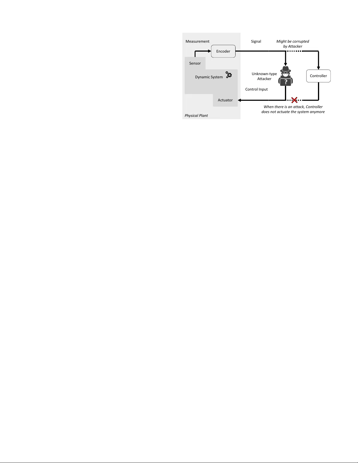
1 Persuasion-based Rob ust Sensor Design Against Attackers with Unkno wn Control Objecti ves Muhammed O. Sayin and T amer Bas ¸ ar , Life F ellow , IEEE Abstract —In this paper , we introduce a rob ust sensor design framework to pro vide “persuasion-based” defense in stochastic control systems against an unknown type attacker with a control objective exclusive to its type. For effective control, such an attacker’ s actions depend on its belief on the underlying state of the system. W e design a rob ust “linear-plus-noise” signaling strategy to encode sensor outputs in order to shape the attacker’s belief in a strategic way and correspondingly to persuade the attacker to take actions that lead to minimum damage with respect to the system’s objective. The speciﬁc model we adopt is a Gauss-Markov process driven by a controller with a (partially) “unknown” malicious/benign contr ol objective. W e seek to defend against the worst possible distribution o ver control objectives in a rob ust way under the solution concept of Stackelberg equilibrium, where the sensor is the leader . W e show that a necessary and sufﬁcient condition on the covariance matrix of the posterior belief is a certain linear matrix inequality and we pro vide a closed-form solution for the associated signaling strategy . This enables us to f ormulate an equi valent tractable problem, indeed a semi-deﬁnite program, to compute the rob ust sensor design strategies “globally” even though the original optimization problem is non-con vex and highly nonlinear . W e also extend this r esult to scenarios where the sensor makes noisy or partial measurements. Finally , we analyze the ensuing performance numerically for various scenarios. Index T erms —Stackelberg games, Stochastic control, Security , Sensor placement, Semi-deﬁnite programming. I . I N T R O D U C T I O N C YBER connectedness of control systems has brought in new security challenges where attackers can manipulate control systems at unprecedented lev els with various malicious tasks on their agenda [1]–[3]. W e can view such intelligent attackers as decision makers that take actions driven by and compatible with their own objecti ve and information available to them. This implies that the kind of information av ailable to an attacker has an indirect impact on what actions the attacker would take. Correspondingly , it is intuitively expected that if we can manipulate the information av ailable to attackers, then we can persuade them to attack the system in a way in line with the system’ s objectiv e to the extent possible, so that the attack would cause minimum damage to the system. There are certain distinct challenges for persuasion-based defense measures. For example, attackers make their decisions based on the belief they hav e formed using the information This research was supported by the U.S. Ofﬁce of Naval Research (ONR) MURI grant N00014-16-1-2710. Muhammed O. Sayin is with Laboratory for Information and Decision Systems at MIT , Cambridge, MA 02139. E-mail: sayin@mit.edu T amer Bas ¸ar is with the Department of Electrical and Computer Engineer- ing, Univ ersity of Illinois at Urbana-Champaign, Urbana, IL 61801 USA. E-mail: basar1@illinois.edu av ailable to them. A challenge is how to shape that belief in a desired way by controlling the information av ailable to the attacker . The ﬁrst requirement (and challenge) here is to be able to identify ho w an attacker would form its belief. Howe ver , when an attacker forms its belief strategically , there might be multiple Nash equilibria in a general-sum setting 1 , as shown in the strate gic information transmission frame work [4]. In that case how an attacker forms its belief is not well deﬁned since the attacker might be forming its belief dif ferently at different equilibria and whether (and which) equilibrium will be realized would not be known, and constitutes an uncer - tainty . Furthermore, even when there exists a well-deﬁned characterization of how an attacker would form its belief, another challenge is what decision the attacker would make based on that belief, since that decision would depend on the attacker’ s malicious objectiv e. This implies that persuasion- based defense is attack-speciﬁc. Therefore another challenge is how to persuade an attacker whose objectiv e is not known to act in a certain way . Before addressing these challenges, let us brieﬂy revie w the literature from a broader perspective where a decision maker seeks to induce another one to take certain actions. A closely related framework is Bayesian persuasion, introduced by Kamenica and Gentzkow in their seminal paper [5]. They addressed ho w a sender could persuade a recei ver to take certain actions under the solution concept of Stackelber g equilibrium [6] where the sender (the receiver) is the leader (the follower). In other words, the recei ver is aware of the sender’ s signaling strate gy while taking its actions. Such a leader-follo wer scheme creates an en vironment where the receiv er’ s actions are not strategic, and therefore there is a well-deﬁned characterization for ho w the belief is formed. In Bayesian persuasion frame work, a necessary and sufﬁ- cient condition is that mean of posterior belief must be equal to the prior belief. This enables us to formulate an equiv alent problem over distributions over posterior beliefs under a linear equality constraint. The authors provided a geometrical interpretation to compute the solution, which necessitates computation of a conv ex env elope of a function. Although this interpretation provides essential insight for designing signaling strategies and has led to various applications (see the recent surve y on Bayesian persuasion [7] and the references therein), it is viable only for scenarios where the state space is very 1 In a zero-sum setting, there exists a unique “babbling equilibrium” where the attacker forms a belief independent of the information provided by a defender (since the defender would not share anything useful) whereas the defender just makes irrelev ant information available to the attacker (since a more informed attacker would not cause less damage to the system). 2 small. W e emphasize that [5] studies the Bayesian persuasion problem in a very general framework, where the underlying distribution is arbitrary as long as its support set is compact, cost functions are arbitrary , and the signaling strategy is any stochastic kernel (between the state space and the signal space). Therefore if we consider speciﬁc distributions and cost functions, we should be able to obtain more tractable solutions. For example in [8], the author addressed Bayesian persuasion problem for multi-v ariate Gaussian information and quadratic cost functions, and provided a closed-form solution for the optimal signaling strategy , which turns out to be a linear function. W e note that the studies [5], [8] focused on static systems. T o be able to adopt this framework to control systems, an important step would be to extend the framew ork to dynamic systems. In [9], we have extended the results in [8] to dynamic en vironments where the underlying information is a discrete-time Gauss Markov process. W e showed that there exists a linear signaling strate gy optimal within the general class of measurable policies and provided a semi-deﬁnite program (SDP) to compute optimal signaling strategies numerically . Before delving into persuasion-based defense measures in control systems, let us also revie w the literature on security of control systems. T o this end, we selectiv ely focus on studies where an attacker can monitor and intervene the links from sensor to controller and from controller to actuator so that there would be an information ﬂow to the attacker who monitors these links. In [10], the authors showed that an attacker can lead to unbounded estimation error by injecting false data into the link from sensor to controller when there exists a certain threshold-based detector monitoring the link. In [11], [12], the authors characterized the reachable set to which an ev asive attacker can drive the system by injecting data into both links jointly . In [13], [14], the authors analyzed attacks where an attacker seeks to dri ve the state of the system according to his/her adversarial goal ev asiv ely by injecting data into both links jointly . In [15], the authors hav e analyzed optimal attack strategies to maximize quadratic cost of a system with linear Gaussian dynamics by injecting false data into the link from controller to actuator without being detected. As seen in the literature revie wed above, an attacker can monitor and intervene the links in a control system, e.g., as illustrated in Fig. 1 for a linear quadratic Gaussian (LQG) control system. This implies that an attacker can bypass the controller of a system by monitoring and interv ening both links jointly . Then the attacker would receive the sensor outputs and could generate its o wn control inputs to conduct its malicious control objectiv e similar to the controller of the system. From this vie wpoint, within the Bayesian persuasion framew ork, we can encode the sensor outputs to persuade the attacker to generate control inputs that w ould minimize the system’ s very own control objectiv e as much as possible. W e partially addressed this challenge in [9], [16], [17]. In [9], we formulated an optimal linear signaling rule in an LQG setting when attack er’ s control objecti ve is kno wn to the sensor . This limits applicability of the solution since the sensor must know when there is an attack and what the control Se nso r Actua t or Dyna mic S y s t em Ph ysic al Plan t Con tr oller Mea sur em en t Signal Con tr ol Input Enc oder ? Unkno wn - type A t t ack er Migh t be c or ru p t ed b y A t t ack er When ther e is an at t ack , Con trolle r do es no t actuat e the s ys t em an ym or e x x x k + 1 = A x x x k + B u u u k + w w w k u u u k = γ k ( s s s 1: k ) y y y k y y y 1: k − 1 s s s k = η k ( y y y 1: k ) Fig. 1: A discrete-time LQG control system where an (unknown-type) attacker can monitor and intervene the links from sensor to controller, and from controller to actuator jointly in order to driv e the system according to its malicious control objectiv e. The attacker might also corrupt the data receiv ed by the controller of the system to e vade a detector monitoring that data. Details of how an attack er can ev ade detection by corrupting that data has earlier been studied in the literature, e.g., [10]–[14], and is out of the scope of this paper since here we focus on adopting persuasion-based defense against attackers with unknown control objecti ves. Furthermore, the results of this paper hold for any strategy that the attacker can use to ev ade such detectors as long as those strategies do not impact how the attacker constructs its control inputs. objectiv e of the attacker is beforehand. In the follow-up papers [16], [17], we sho wed that this limitation could be relaxed in a straightforward way if the sensor knows the distribution ov er the control objectives of attackers that may attack the system and at what probability there might be an attack. Correspondingly , a risk-neutral sensor could minimize the expected damage with respect to that distrib ution. Howe ver , this still limits its applicability since the sensor must kno w the underlying distribution over the attack space. Although it is not a persuasion-based defense, it is worth noting that in [18], the authors proposed linear encoding schemes 2 for sensor outputs in an LQG control problem in order to enhance detectability of false data injection attacks under an essential assumption that the encoding matrix is oblivious to attackers. In that respect, the encoding scheme could be vie wed as corrupting the information av ailable to attackers (without impacting the information ﬂowing to the controller of the system) in order to limit the attacker’ s capability to ev ade detection rather than persuading the at- tacker to attack in a certain way . And this security measure becomes undermined completely once the encoding scheme is compromised. Coming to the speciﬁcs of this paper , we also consider a discrete-time LQG control problem, similar to the studies revie wed abov e [13]–[18], but with important differences. W e 2 W e use the terminologies encoding scheme and signaling rule/strategy interchangeably . 3 particularly seek to design linear -plus-noise signaling rules for persuasion-based rob ust sensor design against an unknown type attacker with a control objectiv e exclusi ve to its type. It is rob ust in the sense that sensor outputs are designed against the worst possible distribution over all possible control objectiv es of the attacker . W e consider the scenario where the set of types is ﬁnite and kno wn to the system. Under the solution concept of Stackelberg equilibrium, we consider the setting where the sensor is the leader and the attacker is the follower . This yields that the underlying encoding scheme is not necessarily oblivious to the attacker . Furthermore, we address the scenarios where the sensor can have partial or noisy measurements dif ferent from the models in [9], [16], [17]. Note that the worst case distribution over the type set turns out to be not necessarily a degenerate distribution, i.e., defending only against the (strongest) type of attack that leads to larges t cost for the system is not necessarily optimal with respect to the system’ s objective. Due to the underlying leader-follower setting, the response of the follower (the attacker) is non-strategic and the problem faced by the leader (the sensor) turns out to be an optimization problem rather than a ﬁxed-point problem. By using the classi- cal method of completion of squares [19], we can show that the objectiv e function in that optimization problem is linear in the cov ariance matrix of the posterior estimate of the underlying (control-free) state. Howe ver that covariance matrix depends on the encoding scheme in a nonlinear way , which leads to a non-con vex and highly nonlinear optimization problem, to be solved globally in order to compute robust sensor design strategies. In [9], our previous inspection rev ealed a necessary condition on this cov ariance matrix, which is just a linear matrix inequality . Here we show that this necessary condition is also a sufﬁcient condition when the sensor selects linear plus noise signaling strategies. Furthermore for any matrix satisfy- ing the necessary condition, we provide a closed-form solution for the associated linear plus noise signaling rule. Therefore instead of trying to solve a non-con vex and highly nonlinear optimization problem, we are able to bring the problem to one of solving a linear optimization problem under linear matrix inequality constraints, which can be done numerically using existing SDP solvers effecti vely , e.g., [20], [21]. This solution concept can be seen to hav e similar ﬂav or with our previous paper [9], revie wed above. Howe ver , here we develop and present a completely new and more comprehensiv e set of technical tools since the results of [9] cannot be adopted for the general setting of this paper . The reader can refer to Appendix A for a detailed discussion on this matter . W e now highlight the main contributions of this paper as follows: • W e show that a necessary and sufﬁcient condition on the cov ariance matrix of the posterior estimate of control- free state is a certain linear matrix inequality . This result is important by itself since it yields a tractable solution concept to design sensor outputs in general settings not limited to the special setting studied in this paper . • Based on this necessary and sufﬁcient condition, we provide an SDP equivalent to the original optimization problem faced by the sensor, which is non-con ve x and highly nonlinear , while the SDP could be solved globally using existing powerful computational tools effecti vely [20], [21]. Furthermore, this result can be extended to scenarios where there are partial or noisy measurements. • W e note that robust signaling rule can dictate sensors to introduce irrelev ant information into sensor outputs quite contrary to other settings, e.g., when there is no uncertainty (or there is imperfect information) on attacker’ s type. This observation enables us to draw the following conclusions: – The equiv alence result does not necessarily hold if the sensor can only use linear signaling rules. – Based on Blackwell’ s Irrele vant Information Theorem [22, Theorem D.1.1], linear signaling strategies are not the best one within the general class of measurable strategies in this robust setting. The paper is organized as follo ws: In Section II, we for- mulate the rob ust sensor design game. In Section III, we analyze the equilibrium of the rob ust sensor design g ame under perfect measurements. In Section IV, we extend the results to the cases where there are partial or noisy measurements. In Section V, we examine numerically the performance of the proposed scheme for v arious scenarios. W e conclude the paper in Section VI with se veral remarks and possible research directions. An appendix provides further discussion on related literature, proofs of all technical results in the order they appear throughout the paper , and some closed-form expressions for the reader’ s reference. Notation: W e denote a collection of parameters via a subscript, e.g., { x k } , by dropping the subscript, e.g., x , for notational brevity . For a vector x and a matrix A , x 0 and A 0 denote their transposes, and k x k denotes the Euclidean ( L 2 ) norm of the v ector x . F or a matrix A , T r { A } and rank { A } denote its trace and rank, respectiv ely . W e denote the identity and zero matrices with the associated dimensions by I and O , respectiv ely . W e denote the set of m -by- m symmetric, positive semi-deﬁnite, and positive deﬁnite matrices by S m , S m + , and S m ++ , respectively . F or a matrix A , A † denotes its Moore- Penrose in verse. For positive semi-deﬁnite matrices A and B , A  B means that A − B is also a positiv e semi-deﬁnite matrix. W e denote the Kroneck er product of matrices A and B by A ⊗ B . W e denote an ordered set { x k , . . . , x 1 } and its augmented vector v ersion,  x 0 k · · · x 0 1  0 , by x 1: k , by some ab use of notation. N ( 0 , . ) denotes the multiv ariate Gaussian distribu- tion with zero mean and designated co variance matrix. W e denote random variables by bold lower case letters, e.g., x x x . W e denote expectation and (co)variance of a random variable x x x by E { x x x } and cov { x x x } , respectively . For random variables x x x and y y y , E { x x x | y y y } denotes the expectation of x x x with respect to the random v ariable y y y . W e denote the set of all possible probability distributions over a set Ω by ∆ ( Ω ) . I I . P RO B L E M F O R M U L A T I O N Consider a control system, as illustrated in Fig. 1, whose underlying state dynamics and sensor measurements are de- 4 scribed, respecti vely , by: x x x k + 1 = A x x x k + B u u u k + w w w k , (1) y y y k = Cx x x k + v v v k , (2) for k = 1 , . . . , κ , where 3 A ∈ R m × m , B ∈ R m × r , and C ∈ R n × m , and the initial state x x x 1 ∼ N ( 0 , Σ 1 ) . The additi ve state and measurement noise sequences { w w w k } and { v v v k } , respectively , are white Gaussian vector processes, i.e., w w w k ∼ N ( 0 , Σ w ) and v v v k ∼ N ( 0 , Σ v ) ; and are independent of the initial state x x x 1 and of each other . As seen in Fig. 1, measurements y y y 1: k ∈ R nk are encoded into a signal s s s k ∈ R m through a signaling strate gy η k ( · ) , which is a stochastic kernel, and s s s k = η k ( y y y 1: k ) almost everywhere ov er R m . W e speciﬁcally consider “linear plus noise” signaling rules such that the signal s s s k is gi ven by s s s k = η k ( y y y 1: k ) = L 0 k y y y 1: k + ϑ ϑ ϑ k , (3) almost ev erywhere over R m , where L k ∈ R nk × m can be any nk -by- m deterministic matrix, and ϑ ϑ ϑ k ∼ N ( 0 , Θ k ) is a zero mean multiv ariate Gaussian noise independent of every other parameter , and its cov ariance matrix Θ k ∈ S m + can be any m - by- m positiv e semi-deﬁnite matrix. W e denote the set of such signaling rules by ϒ k , i.e., η k ∈ ϒ k . Furthermore, the closed- loop control input u u u k ∈ R r is gi ven by u u u k = γ k ( s s s 1: k ) , (4) almost ev erywhere ov er R r , where γ k ( · ) can be any Borel measurable function from R mk to R r . W e denote the set of such control policies by Γ k , i.e., γ k ∈ Γ k . For notational bre vity , let us denote signaling (control) strategies and the associated sets across the horizon by η and ϒ ( γ and Γ ), respectiv ely . A. Defense Model W e consider an LQG control problem, where the controller of the system selects a measurable control strategy γ ∈ Γ in order to minimize κ ∑ k = 1 E k x x x k + 1 k 2 Q + E k u u u k k 2 R , (5) where 4 Q ∈ S m + and R ∈ S r ++ . As illustrated in Fig. 1, we consider the encoder of the system as a decision maker , denoted by P S . P S selects the signaling strategy η ∈ ϒ in order to minimize the same objectiv e with the controller , (5). Note that if there were no attacks, identity function, where the measurements are shared with the controller fully , would be an optimal encoding scheme due to the data processing inequality [23, Theorem 2.8.1]. Ho wev er , we consider here the scenarios where there can be an attack with an unknown control objective. Correspondingly there might be encoding schemes that do not share the measurements fully and can lead to better performance with respect to (5). 3 Even though we consider time-in variant matrices A , B , and C , for notational simplicity , the provided results could be extended to time-variant cases rather routinely . Furthermore, we consider all the random parameters to have zero mean; howe ver , the deriv ations can be extended to non-zero mean case in a straight-forward way . 4 For notational simplicity , we consider time-inv ariant Q and R . Howev er, the results pro vided could be extended to the general time-variant case rather routinely . B. Attack Model W e consider an attack er who is aware of the underlying state dynamics, i.e., gain matrices A , B , and C ; covariance matrices Σ 1 , Σ w , and Σ v ; and the encoding scheme, i.e., η . The attacker is of an unknown type, which determines its control objecti ve. Let us denote the set of all possible types by Ω . W e suppose that Ω is ﬁnite and known by the system. W e seek to provide a compact and uniﬁed analysis. Therefore we consider that the control objecti ve of type ω ∈ Ω is given by κ ∑ k = 1 E k x x x ω k + 1 k 2 Q ω + E k u u u ω k k 2 R ω , (6) where Q ω ∈ S m + and R ω ∈ S r ++ are exclusi ve to the type ω . Note that when there is an attack, the attacker selects a control strategy γ ω ∈ Γ in order to construct its control input u u u ω k and correspondingly its control objectiv e includes the term E k u u u ω k k 2 R ω . W e also denote the state driv en by type- ω attacker by x x x ω k , to make it explicit. Remark 1 (V ersatility of Control Objectives) . W e model the control objectives of the system and the attacker by (5) and (6), respectiv ely , within a uniﬁed framework. Howe ver , arbi- trariness of weight matrices in the control objecti ves (5) and (6) brings in ﬂexibility to model various attack scenarios (that are not in the exact form of (6)) through the transformation of the underlying state space as ex empliﬁed in Section V.  C. Game Model W e analyze the interaction between the attacker and P S under the solution concept of Stackelber g equilibrium where P S is the leader . Note that from the viewpoint of P S , either the controller of the system is receiving the sensor output and driving the state or there is an unknown type attack, and it is getting the sensor output and it is generating the control input. Since whether there is an attack or not is also an uncertainty , let us view the attacker and the controller of the system as a single player in a uniﬁed way , denoted by P C , with an unknown type from the extended type set Ω o : = Ω ∪ { ω o } , where type- ω o corresponds to the controller of the system, i.e., Q ω o = Q and R ω o = R . Therefore, we consider a Stackelberg game between the leader P S and the follo wer P C (of an unknown type). W e note that depending on its type, P C selects dif ferent control policies, which lead to different control inputs, and states. Therefore for type- ω P C , we use γ ω k , x x x ω k and u u u ω k . The objectiv e of type- ω P C is gi ven by U ω C ( η , γ ω ) : = κ ∑ k = 1 E k x x x ω k + 1 k 2 Q ω + E k u u u ω k k 2 R ω . (7) On the other hand, the objecti ve of P S is gi ven by U S ( η , { γ ω } ω ∈ Ω o ) : = max p ∈ ∆ ( Ω o ) ( ∑ ω ∈ Ω p ω κ ∑ k 0 = 1 E k x x x ω k 0 + 1 k 2 Q ω o + p ω o κ ∑ k = 1  E k x x x ω o k + 1 k 2 Q ω o + E k u u u ω o k k 2 R ω o  ) , (8) 5 where ∆ ( Ω o ) denotes all possible distrib utions over the ex- tended type set Ω o . Note that the maximization in (8) computes the cost of P S for the worst case distribution ov er Ω o . Before describing the game formally , let us take a closer look at P S ’ s objectiv e (8). W e can view (8) consisting of two parts, one of which is p ω o κ ∑ k = 1  E k x x x ω o k + 1 k 2 Q ω o + E k u u u ω o k k 2 R ω o  , (9) where p ω o corresponds to the probability that the controller of the system driv es the state under the worst case distribution and the summation is identical to (5) since Q ω o = Q and R ω o = R . The other part is ∑ ω ∈ Ω p ω κ ∑ k 0 = 1 E k x x x ω k 0 + 1 k 2 Q ω o , (10) which implies that P S seeks to minimize ∑ κ k = 1 E k x x x ω k + 1 k 2 Q ω o when type- ω attacker dri ves the state. Note that it includes only the ﬁrst term in (5) since we consider that P S would not necessarily want the attacker to have small size control inputs. Deﬁnition (Robust Sensor Design Game) . The robust sensor design game G : = ( ϒ , Γ , x x x 1 , w w w 1: κ , v v v 1: κ ) (11) is a Stackelber g game between the leader P S and the follo wer P C . Objectiv es of P C and P S are giv en by (7) and (8), respectiv ely . Then a tuple of strategies ( η , { γ ω } ω ∈ Ω o ) attains the Stackelber g equilibrium provided that η ∈ argmin η 0 ∈ ϒ U S  η 0 , { γ ω ( η 0 ) } ω ∈ Ω o  (12a) γ ω ( η ) ∈ ar gmin γ ∈ Γ U ω C  η , γ ( η )  . (12b) where, by an abuse of notation, we denote type- ω P C ’ s strat- egy γ ω by γ ω ( η ) to show its dependence on P S ’ s signaling rules due to the leader-follo wer scheme, explicitly . Note that there might be multiple best responses by P C for a signaling strategy . Correspondingly (12a) would not be well deﬁned if these best responses lead to different costs for P S . Howe ver , as we will show later in detail, reaction set of type- ω P C turns out to be an equiv alence class such that all γ ω in the reaction set lead to the same control input almost surely , and correspondingly lead to the same cost for P S . I I I . R O B U S T S E N S O R D E S I G N F R A M E W O R K In this section, we consider the special case where P S has access to perfect measurements, i.e., y y y k = x x x k for k = 1 , . . . , κ ; the general noisy/partial measurements case will be addressed later in Section IV. T o compute the equilibrium of the game G , we ﬁrst focus on best response strategy of P C for a giv en sig- naling strategy . This enables us to formulate the optimization problem faced by P S to compute robust signaling strategies. Even though this is a ﬁnite-dimensional optimization problem, further inspection reveals that it is highly nonlinear and non- con vex. Therefore a generic approach would not be able to address it globally . T o mitigate this issue, we formulate a tractable problem equiv alent to the original optimization problem. W e can solve this tractable problem globally using existing computational tools effecti vely . Giv en that solution, we also show how we can compute the associated signaling strategies. W e now provide the details of these steps. An important challenge in the design of encoding schemes in control systems compared to communication systems is that the underlying state depends on control inputs. T o mitigate this issue, we introduce control-free state { x x x o k } ev olving according to x x x o k + 1 = A x x x o k + w w w k , (13) and x x x o 1 = x x x 1 . As sho wn in [24], the routine technique of completion of squares yields that κ ∑ k = 1 E k x x x k + 1 k 2 Q ω + E k u u u k k 2 R ω = κ ∑ k = 1 E k u u u o k + K ω k x x x o k k 2 ∆ ω k + δ ω 0 , (14) where the matrices K ω k , ∆ ω k , and scalar δ ω o are gi ven by K ω k = ( ∆ ω k ) − 1 B 0 ˜ Q ω k + 1 A ∆ ω k = B 0 ˜ Q ω k + 1 B + R ω δ ω 0 = T r { Q ω Σ 1 } + κ ∑ k = 1 T r { ˜ Q ω k + 1 Σ w } and { ˜ Q ω k } satisﬁes the follo wing discrete-time dynamic Riccati equation ˜ Q ω k = Q ω + A 0 ( ˜ Q ω k + 1 − ˜ Q ω k + 1 B ( ∆ ω k ) − 1 B 0 ˜ Q ω k + 1 ) A and ˜ Q ω κ + 1 = Q ω . Furthermore u u u o k depends on the control inputs through the follo wing transformation: u u u o k = u u u k + K ω k B u u u k − 1 + . . . + K ω k A k − 2 B u u u 1 . Note that ∆ ω k is positi ve deﬁnite for all k . Contrary to team problems (where all decision makers hav e the same objecti ve), as studied in [24], in non cooperativ e settings, (14) does not imply that a control input leading to u u u o k = − K ω k E { x x x o k | s s s 1: k } is optimal since control inputs can have an impact on the signals that will be generated in future stages. Howe ver , as we will sho w below , P C cannot impact the signals generated in future stages when P S uses linear plus noise signaling strategies only . T o show this, we let the gain matrix L k ∈ R nk × m in signaling strategy η k , as described in (3), be partitioned as L k =  L 0 k , k · · · L 0 k , 1  0 , where L k , j ∈ R n × m . Then, signal s s s k can be written as L 0 k , k x x x k + . . . + L 0 k , 1 x x x 1 + ϑ ϑ ϑ k = L 0 k , k x x x o k + . . . + L 0 k , 1 x x x o 1 + ϑ ϑ ϑ k + n L 0 k , k B u u u k − 1 + . . . + ( L 0 k , k A k − 2 + . . . + L 0 k , 2 ) B u u u 1 o , where the term in-between {·} is σ - s s s 1: k − 1 measurable. Similar to 5 [9, Lemma 12], this yields that E { x x x o k | s s s 1: k } = E { x x x o k | s s s o 1: k } , (15) where we deﬁne s s s o k : = L 0 k x x x o 1: k + ϑ ϑ ϑ k . Correspondingly , since ∆ ω k is positive deﬁnite for all k , right-hand sides of (14) and (15) yield that optimal reaction of type- ω P C is indeed the one that leads to u u u o k = − K ω k E { x x x o k | s s s 1: k } , (16) 5 W e note that [9, Lemma 12] shows a result similar to (16) when the sender selects only linear and memoryless signaling strategies. 6 almost ev erywhere over R r , since E { x x x o k | s s s 1: k } does not depend on u u u 1: k . This sho ws that all strategies in the best reaction set of type- ω P C lead to (16) and therefore lead to the same cost for P S . Based on (16), the follo wing lemma sho ws that we can write the optimization objective in (8) as a linear function of the cov ariance matrix of the posterior estimate of control-free state, i.e., 6 H k : = cov { E { x x x o k | s s s 1: k }} , for k = 1 , . . . , κ . Lemma 1. The pr oblem faced by P S , i.e., (12a) , can be written as min η ∈ ϒ max p ∈ ∆ ( Ω o ) ∑ ω ∈ Ω o p ω ξ ω + κ ∑ k = 1 T r { H k Ξ ω k } ! , (17) wher e Ξ ω k is a certain symmetric matrix, described in (50) , that does not depend on the optimization ar guments, and ξ ω ∈ R , described in (44) and (49) , is a certain ﬁxed scalar . W e emphasize that complexity of the objectiv e functions (5) and (8) is buried in ﬁxed parameters {{ Ξ ω k } , ξ ω } . Based on this observ ation, we make the following remarks: Remark 2 (V ersatility of the results with respect to P C ’ s objectiv e) . The problem faced by P S is a linear function of the cov ariance matrices { H k } since optimal reaction of P C turns out to be linear in the posterior estimate of the control-free state, i.e., E { x x x o k | s s s 1: k } , as seen in (16). Therefore the results henceforth hold for any other scenarios where P C has any other objectiv e in which optimal reaction of P C still turns out to be a linear function of the posterior estimate. Note that we need to compute the associated {{ Ξ ω k } , ξ ω } accordingly .  Remark 3 (V ersatility of the results with respect to P S ’ s objectiv e) . W e motiv ate and consider the case where P S has objectiv e (8). Howe ver , the results henceforth would also hold for scenarios where P S ’ s objecti ve is any other (con vex or non-con vex) quadratic function of the state and control input. Note that we also need to compute the associated {{ Ξ ω k } , ξ ω } accordingly .  Compared to original form of the optimization problem (12a), the optimization problem (17) has a concrete structure showing that the optimization function depends on the sig- naling strategy through the cov ariance matrix only , and it is a linear function of the cov ariance matrix. Therefore it is instruc- tiv e to study the relationship between the cov ariance matrix and the signaling strategy . Since the underlying distributions are all jointly Gaussian, we can express the cov ariance matrix in closed form: H k = E { x x x o k s s s 0 1: k } E { s s s 1: k s s s 0 1: k } † E { x x x o k s s s 0 1: k } 0 (18) and the signal s s s k is given by (3). This yields that even though computing rob ust signaling strategies would mean ﬁnding a 6 Henceforth we say “covariance matrix” instead of “cov ariance matrix of posterior estimate of control-free state”, and we say “posterior” instead of “posterior estimate of control-free state”. certain number of matrices, it is a highly nonlinear and non- con vex optimization problem due to the matrix in version in (18). Therefore it is difﬁcult to obtain a global solution through a generic attempt, e.g., genetic algorithm [25] or particle swarm optimization [26]. On the other hand, the follo wing proposition shows that there is a computationally tractable relationship between the cov ariance matrix and linear plus noise signaling strategies. Proposition 1 (A Necessary and Sufﬁcient Condition) . F or any signaling rule η ∈ ϒ , covariance matrix of posterior estimate of the contr ol-free state, { H k = cov { E { x x x o k | s s s 1: k }}} , satisﬁes Σ o 1  H 1  O , (19a) Σ o k  H k  AH k − 1 A 0 , for k > 1 , (19b) wher e 7 Σ o k : = E { x x x o k ( x x x o k ) 0 } . Furthermor e for any collection of positive semi-deﬁnite matrices S 1: κ satisfying Σ o 1  S 1  O , (20a) Σ o k  S k  AS k − 1 A 0 , for k > 1 , (20b) ther e exists a (memoryless) linear-plus-noise signaling strat- e gy 8 η ∈ ϒ such that S k = H k . In the following, we pro vide a description of signaling strategies 9 that lead to covariance matrices matching with a giv en collection of positi ve semi-deﬁnite matrices S 1: κ satis- fying (35). T o this end, we let Σ o k − AS k − 1 A 0 = ¯ U k  ¯ Λ k O O O  ¯ U 0 k be the eigen-decomposition such that ¯ Λ k ∈ S t k ++ , where t k = rank { Σ o k − AS k − 1 A 0 } . Furthermore, we let T k : = h ¯ Λ 1 / 2 k O i ¯ U 0 k ( S k − AS k − 1 A 0 ) ¯ U k  ¯ Λ 1 / 2 k O  hav e the eigen-decomposition T k = U k Λ k U 0 k with eigen values, e.g., λ k , 1 , . . . , λ k , t k . W e note that λ k , t turns out to be in [ 0 , 1 ] . Then, the associated signaling strategy is giv en by s s s k = L 0 k , k x x x k + ϑ ϑ ϑ k , (21) where ϑ ϑ ϑ k ∼ N ( 0 , Θ k ) with Θ k = diag { θ 2 k , 1 , . . . , θ 2 k , t k , 0 , . . . , 0 } , and the gain matrix L k , k is gi ven by L k , k = ¯ U k  ¯ Λ − 1 / 2 k U k Λ o k O O O  , where Λ o k : = diag { λ o 1 , 1 , . . . , λ o 1 , t k } is a diagonal matrix such that { λ o k , i , θ 2 k , i } t k i = 1 satisﬁes ( λ o k , i ) 2 ( λ o k , i ) 2 + θ 2 k , i = λ k , i , ∀ i = 1 . . . . , t k . 7 By the deﬁnition of Σ o k , we have Σ o k = A Σ o k A 0 + Σ w . 8 Such a signaling strategy is described in (21) later . 9 A derivation of the associated signaling strategies can be found in the constructiv e proof of Proposition 1, which is provided in Appendix C. 7 The following corollary to Proposition 1 provides a problem equiv alent to (17). Corollary 1 (Equiv alence Result) . The pr oblem faced by P S , i.e., (8) , is equivalent to min { S k ∈ S m + } max p ∈ ∆ ( Ω o ) ∑ ω ∈ Ω o p ω ξ ω + κ ∑ k = 1 T r { S k Ξ ω k } ! , (22) subject to the following linear matrix inequalities: Σ o 1  S 1  O (23a) Σ o k  S k  AS k − 1 A 0 , for k > 1 . (23b) And given a solution S 1: κ , an associated signaling strate gy can be computed accor ding to (21) . Henceforth, we will be working with (22) instead of (17) while analyzing the equilibrium of the game G . Furthermore, for bre vity of presentation, let us introduce S : =    S κ . . . S 1    , Ξ ω : =    Ξ ω κ . . . Ξ ω 1    , and Ψ ⊂ S m κ + be the set corresponding to the constraints (23) in this new high-dimensional space, i.e., R m κ × m κ . With this new notation, the problem faced by P S , i.e., (22), can be written as min S ∈ Ψ max p ∈ ∆ ( Ω o ) ∑ ω ∈ Ω o p ω ( ξ ω + Tr { S Ξ ω } ) . (24) The follo wing proposition addresses the existence of an equilibrium for the game G . Proposition 2 (Existence Result) . Ther e exists at least one tuple of strate gies ( η , { γ ω ( η ) } ω ∈ Ω o ) attaining the equilibrium of the Stack elberg game G , i.e., satisfying (12) . It is instructi ve to examine whether optimal signaling strate- gies end up using irrele vant information or not. The inner optimization problem in (24) max p ∈ ∆ ( Ω o ) ∑ ω ∈ Ω o p ω ( ξ ω + Tr { S Ξ ω } ) (25) is a con vex function of S ∈ Ψ since the maximum of any family of linear/afﬁne functions is a conv ex function [27]. Therefore, there might be examples where any extreme point of the constraint set Ψ is not a solution for (24). Correspond- ingly , optimal signaling strategy can turn out to be including irrelev ant information. This is interesting in view of Black- well’ s Irrelev ant Information Theorem [22, Theorem D.1.1]. Particularly , the theorem says that giv en a cost measure, for any Borel measurable function that uses irrele vant information, there exists another Borel measurable function that does not use any irrelev ant information and can lead to a cost less than or equal to the one attained with the former function. Therefore we can conclude that in this robust setting, linear signaling strate gies are not the best one within the general class of measurable strategies. Next, we seek to compute the equilibrium of G . T o this end, we examine the equilibrium conditions further . In particular, according to (24), gi ven S ∈ Ψ , maximizing p ∗ ∈ ∆ ( Ω o ) is giv en by p ∗ ∈  p ∈ ∆ ( Ω o ) | p ω = 0 provided that ( ξ ω + Tr { S Ξ ω } ) < max ω 0  ξ ω 0 + Tr { S Ξ ω 0 }   (26) since the optimization objectiv e in (24) is a linear function of p ∈ ∆ ( Ω o ) . Based on the observation (26) and the assumption that the type set Ω o is ﬁnite, the following theorem provides an algorithm to compute robust sensor outputs. Theorem 1 (Computing the Equilibrium) . The value of the Stack elberg equilibrium (24) is given by µ = min ω ∈ Ω o { µ ω } , wher e µ ω : = min S ∈ Ψ  ξ ω + Tr  Ξ ω S  (27) s . t . T r  S ( Ξ ω − Ξ ω 0 )  ≥ ξ ω 0 − ξ ω ∀ ω 0 ∈ Ω o . Furthermor e, let µ ω ∗ = µ and S ∗ ∈ argmin S ∈ Ψ  ξ ω + Tr  Ξ ω S  (28) s . t . T r  S ( Ξ ω − Ξ ω 0 )  ≥ ξ ω 0 − ξ ω ∀ ω 0 ∈ Ω o . Then, given S ∗ ∈ Ψ , an associated linear-plus-noise signaling strate gy η ∈ ϒ can be computed accor ding to (21) . For the reader’ s reference, in the following, we list the steps to compute robust sensor design strategies: • W e ﬁrst compute the matrices Ξ ω k , described in (50), and scalars ξ ω , described in (44) and (49), for each type of control objectiv es, ω ∈ Ω o . This step includes computation of gain matrices of optimal control input, e.g., (16), in an LQG control problem. • Giv en computed {{ Ξ ω k , ξ ω }} , we solve SDP , described in (27), for each type by using an SDP solver , e.g., [20], [21], numerically . • When we compute S ∗ according to (28), we can com- pute the associated signaling strategies according to (30). Note that this step includes computation of eigen- decomposition of some matrices. W e re-emphasized that we provide an algorithm to compute robust signaling strategies globally ev en though the problem is highly nonlinear and non-con vex. There is, howe ver , still room to develop computationally more efﬁcient approaches. And the solution concept proposed in the paper can be used as a benchmark to ev aluate performance of such computationally efﬁcient algorithms. I V . N O I S Y O R P A RT I A L M E A S U R E M E N T S In this section, we seek to obtain robust signaling strategies under noisy or partial (i.e., imperfect) measurements of the type (2). T o this end, we turn the problem to the same structure with the case under perfect measurements based on a recent result from [28] and then inv oke the results from the previous section. There are se veral challenges in robust sensor design under imperfect measurements. For e xample, Proposition 1 does 8 not hold anymore. T o obtain a result similar to Proposition 1, a ﬁrst attempt would be to focus on the cov ariance ma- trix of the posterior estimate of control-free measurements , i.e., cov { E { y y y o k | s s s 1: k }} , where y y y o k : = C x x x o k + v v v k , instead of H k = cov { E { x x x o k | s s s 1: k }} . Quite contrary to the control-free state { x x x o k } , howe ver , control-free measurements { y y y o k } do not necessarily constitute a Markov process since in general E { y y y o k | y y y o 1: k − 1 } 6 = E { y y y o k | y y y o k − 1 } . Therefore, we focus on the augmented vector of measurements y y y o 1: k ∈ R nk . Since the measurements are jointly Gaussian, we have E { y y y o k | y y y o 1: k − 1 } = E { y y y o k ( y y y o 1: k − 1 ) 0 } E { y y y o 1: k − 1 ( y y y o 1: k − 1 ) 0 } † y y y o 1: k − 1 . This implies that the augmented measurements { y y y 1: k } k ≥ 0 ev olve according to y y y o 1: k = A k y y y o 1: k − 1 + e e e k , (29) where we deﬁne A k : =  E { y y y o k ( y y y o 1: k − 1 ) 0 } E { y y y o 1: k − 1 ( y y y o 1: k − 1 ) 0 } † I  , e e e k : =  y y y o k − E { y y y o k | y y y o 1: k − 1 } 0  Note that neither A k ∈ R nk × n ( k − 1 ) nor e e e k ∈ R nk depend on signaling or control strategies. Furthermore, similar to (15), it can be sho wn that E { y y y o 1: k | s s s 1: k } = E { y y y o 1: k | s s s o 1: k } , (30) where we no w have s s s o k = L 0 k y y y o 1: k + ϑ ϑ ϑ k . Since s s s o 1: k is σ - y y y 1: k measurable, x x x o k and s s s o 1: k are independent of each other conditioned on y y y o 1: k . This implies that x x x o k , y y y o 1: k , and s s s o 1: k can be viewed as forming a Markov chain in the order x x x o k → y y y o 1: k → s s s o 1: k . In that respect, [28, Lemma 1] shows that when { x x x o k , y y y o 1: k , s s s 1: k } are jointly Gaussian and form a Markov chain in the order x x x o k → y y y o 1: k → s s s o 1: k , there exists a linear relation between E { x x x o k | s s s o 1: k } and E { y y y o 1: k | s s s o 1: k } irrespective of s s s o 1: k , and the relation is gi ven by E { x x x o k | s s s o 1: k } = D k E { y y y o 1: k | s s s o 1: k } , (31) where D k ∈ R m × nk is deﬁned by D k : = E { x x x o k ( y y y o 1: k ) 0 } E { y y y o 1: k ( y y y o 1: k ) 0 } † . Under imperfect measurements, counterpart of the covari- ance matrix H k = cov { E { x x x o k | s s s 1: k }} is the covariance matrix of the posterior estimate of control-free augmented measure- ments, denoted by Y k : = cov { E { y y y o 1: k | s s s 1: k }} . Based on (30) and (31), we ha ve H k = D k Y k D 0 k . Correspondingly , (17), i.e., the problem faced by P S , can be written as min η ∈ ϒ max p ∈ ∆ ( Ω o ) ∑ ω ∈ Ω o p ω ξ ω + κ ∑ k = 1 T r { Y k W ω k } ! , (32) where we deﬁne 10 W ω k : = D 0 k Ξ ω D k , which can be vie wed as the counterpart of Ξ ω k under imperfect measurements. W e remark the resemblance between (17) and (32), where we have Y k instead of H k and W ω k instead of Ξ ω k . Recall that y y y k ∈ R n , which yields that y y y 1: k ∈ R nk . Under the assumption that s s s k ∈ R nk instead of s s s k ∈ R m (so that P S can disclose the auxiliary y y y 1: k perfectly), we would hav e transformed the problem under imperfect measurements into a problem under perfect measurements, and correspondingly we could have in vok ed the results from the previous section directly . The following lemma shows that results for the case where s s s k ∈ R nk would also hold for the case where s s s k ∈ R m ev en when nk > m . Lemma 2. Let us denote signaling strate gies when s s s k ∈ R nk by ˜ η k and the associated strate gy space by ˜ ϒ k . Then for any { ˜ η k ∈ ˜ ϒ k } , there exists a { η k ∈ ϒ k } such that they both lead to the same contr ol strate gy and correspondingly the same cost for P S . And such a signaling strate gy { η k ∈ ϒ k } is given by η k ( y y y 1: k ) = E { x x x o k | ˜ η 1 ( y y y 1 ) , . . . , ˜ η k ( y y y 1: k ) } , ∀ k ≥ 1 . (33) Based on Lemma 2, the following corollary to Proposition 1 provides a tractable necessary and suf ﬁcient condition on { Y k } . Corollary 2 (A Necessary and Suf ﬁcient Condition Under Imperfect Measurements) . F or any signaling rule η ∈ ϒ , covariance matrix of posterior estimate of the contr ol-free measur ements, { Y k = cov { E { y y y o 1: k | s s s 1: k }}} , satisﬁes Σ y 1  Y 1  O , (34a) Σ y k  Y k  A k − 1 Y k − 1 A 0 k − 1 , for k > 1 , (34b) wher e Σ y k : = E { y y y o 1: k ( y y y o 1: k ) 0 } . Furthermor e for any collection of positive semi-deﬁnite matrices S 1: κ satisfying Σ y 1  S 1  O , (35a) Σ y k  S k  A k − 1 S k − 1 A 0 k − 1 , for k > 1 , (35b) ther e exists a linear-plus-noise signaling strate gy η ∈ ϒ such that S k = Y k . The follo wing corollary provides a problem equi valent to (32). Corollary 3. The pr oblem faced by P S , i.e ., (32) , is equivalent to min { S k ∈ S kn + } max p ∈ ∆ ( Ω o ) ∑ ω ∈ Ω o p ω ξ ω + κ ∑ k = 1 T r { S k W ω k } ! , (36) subject to the following linear matrix inequalities: Σ y 1  S 1  O , (37a) Σ y k  S k  A k − 1 S k − 1 A 0 k − 1 , for k > 1 . (37b) Furthermor e, given as solution { S 1: κ } for (36) , we can compute an optimal signaling strate gy for (32) , as follows: • Compute signaling strate gies ˜ η ∈ ˜ ϒ as if signal s s s k can be nk dimensional, i.e., s s s k ∈ R nk , according to (21) , where 10 W e use the cyclic property of the trace operator . 9 we have Σ y k instead of Σ o k , A k instead of A, and y y y 1: k instead of x x x k . 11 • F or computed ˜ η ∈ ˜ ϒ , compute associated signaling str ate- gies η ∈ ϒ according to (33) . W e remark that under imperfect measurements optimal signaling strategies are not necessarily memoryless anymore. Through a similar notational con vention as in the previous section, we can write (36) as min S ∈ ¯ Ψ max p ∈ Ω o ∑ ω ∈ Ω o p ω ( ξ ω + Tr { S W ω } ) , (38) where we let ¯ Ψ ⊂ S m κ ( κ + 1 ) / 2 be the set corresponding to the constraints (37). Then, based on Corollary 3, the follo wing corollary to Theorem 1 provides a computationally tractable way to compute robust sensor outputs under imperfect mea- surements. Corollary 4 (Computing the Equilibrium Under Imperfect Measurements) . The value of the Stackelber g equilibrium (38) is given by µ = min ω ∈ Ω o { µ ω } , wher e µ ω : = min S ∈ ¯ Ψ  ξ ω + Tr  W ω S  (39) s . t . T r  ( W ω − W ω 0 ) S  ≥ ξ ω 0 − ξ ω ∀ ω 0 ∈ Ω o . Furthermor e, let µ ω ∗ = µ and S ∗ ∈ argmin S ∈ ¯ Ψ  ξ ω + Tr  W ω S  (40) s . t . T r  ( W ω − W ω 0 ) S  ≥ ξ ω 0 − ξ ω ∀ ω 0 ∈ Ω o . Then, given S ∗ ∈ ¯ Ψ , an associated linear-plus-noise signaling strate gy η ∈ ϒ can be computed accor ding to Corollary 3. V . I L L U S T R AT I V E E X A M P L E S In this section, we examine the performance of the proposed defense measure over various attack scenarios. As an illustra- tiv e example, we set length of the time horizon at κ = 10, dimension of state m = 2, and dimension of control input r = 2. W e consider the scenario where the system’ s control objectiv e is to track an exogenous process { z z z k } e volving according to z z z k + 1 = A z z z z k + w w w z k , where z z z 1 ∼ N ( 0 , I 2 ) , and { w w w z k ∼ N ( 0 , I 2 ) } is a white Gaussian noise process, and they are independent of each other and ev ery other parameter . Correspondingly , the system’ s control objectiv e can be written as U ω o C ( η , γ ω o ) = κ ∑ k = 1 E k x x x ω o k + 1 − z z z k + 1 k 2 + E k u u u ω o k k 2 . (41) W e set A = A z = I 2 and B =  1 1 0 1  while Σ 1 = I 2 and Σ w = I 2 . The sensor has access to the measurements: y y y k = Cx x x k + v v v k y y y z k = C z z z z k + v v v z k , 11 W e provide closed-form expressions for the auxiliary parameters Σ y k , A k , and D k in Appendix G for the reader’ s reference. where { v v v z k } is a white Gaussian measurement noise indepen- dent of e very other parameter . Note that the control objectiv e is not in the form of (5); howe ver , we can transform it into the form of (5) by intro- ducing the augmented state ˜ x ˜ x ˜ x k : =  x x x 0 k z z z 0 k  0 ev olving according to  x x x k + 1 z z z k + 1  =  I O O I   x x x k z z z k  +  I O  u u u k +  w w w k w w w z k  and augmented measurements are then gi ven by ˜ y ˜ y ˜ y k =  C O O C z   x x x k z z z k  +  v v v k v v v z k  . Correspondingly (41) can be written as κ ∑ k = 1 E k ˜ x ˜ x ˜ x k + 1 k 2 Q + E k u u u k k 2 , where Q : =  I 2 − I 2   I 2 − I 2  . As e xamples of attack scenarios, we consider a type set Ω = { ω a , ω b , ω c } . Let us partition the underlying state x x x k =  x x x k , 1 x x x k , 2  0 and the exogenous process z z z k =  z z z k , 1 z z z k , 2  0 , where x x x k , 1 and z z z k , 1 (or x x x k , 2 and z z z k , 2 ) correspond to the ﬁrst (or the second) entries of the state and the exogenous process, respectiv ely . W e assume that type- ω a attacker seeks to make { x x x k , 1 } track {− z z z k , 1 } instead of { z z z k , 1 } whereas it is not interested in { x x x k , 2 } . Then its control objectiv e can be written as U ω a C ( η , γ ω a ) = κ ∑ k = 1 E k x x x ω a k + 1 , 1 − ( − z z z k + 1 , 1 ) k 2 + E k u u u ω a k k 2 . Similarly type- ω b attacker seeks to make { x x x k , 2 } track {− z z z k , 2 } instead of { z z z k , 2 } whereas it is not interested in { x x x k , 1 } . Then its control objecti ve can be written as U ω b C ( η , γ ω b ) = κ ∑ k = 1 E k x x x ω b k + 1 , 2 − ( − z z z k + 1 , 2 ) k 2 + E k u u u ω b k k 2 . On the other hand, type- ω c attacker is interested in both entries and seeks to make the entire state { x x x k } track {− z z z k } . Accordingly , its control objective can be written as U ω c C ( η , γ ω c ) = κ ∑ k = 1 E k x x x ω c k + 1 − ( − z z z k + 1 ) k 2 + E k u u u ω c k k 2 . W e note that numerical simulations show that mixtures of types ω a , ω b and ω c can lead to larger costs for the system than any single type, including type- ω c . In the following, we examine the cost of P S under perfect and imperfect measurements separately . Under perfect measurements, the sensor has access to ˜ y ˜ y ˜ y k = ˜ x ˜ x ˜ x k . Note that perfect measurements provide the utmost fr eedom for P S to shape the belief of the attacker . For any cost that P S can attain under imperfect measurements, P S can select a signaling strategy under perfect measurements to attain the same cost. Therefore, P S attains the lowest possible cost under perfect measurements in the robust sensor design framew ork. In T able I, we tab ulate the cost to P S for the scenarios where i ) there is no attack, i.e., type of P C is ω o ; ii ) there 10 T ABLE I: Under perfect measurements, i.e., ˜ y ˜ y ˜ y k = ˜ x ˜ x ˜ x k , com- parison of the costs to P S , i.e., U S as described in (8), over various scenarios. Entries at each row corresponds to the cost to P S for different types of P C when it constructs the sensor outputs according to the extended type set Ω o . And the last column provides the maximum cost of P S across all types of P C . Ω o ω o ω a ω b ω c Max { ω o } 43 . 03 323 . 70 354 . 02 352 . 65 354 . 02 { ω a } 122 . 31 191 . 12 351 . 85 246 . 30 351 . 85 { ω b } 119 . 09 320 . 81 185 . 63 267 . 35 320 . 81 { ω c } 106 . 26 202 . 40 224 . 77 137 . 71 224 . 77 { ω o , ω a } 119 . 65 191 . 12 351 . 11 245 . 95 351 . 11 { ω o , ω b } 115 . 29 321 . 56 185 . 63 267 . 93 321 . 56 { ω o , ω c } 106 . 26 202 . 40 224 . 77 137 . 71 224 . 77 { ω o , ω a , ω b , ω c } 81 . 17 199 . 46 199 . 46 166 . 68 199 . 46 is an attack by type- ω a attacker , i.e., type of P C is ω a ; iii ) there is an attack by type- ω b attacker , i.e., type of P C is ω b ; and iv ) there is an attack by type- ω c attacker , i.e., type of P C is ω c . Cost to P S varies depending on the type of P C and how prepared P S is while constructing the sensor outputs. In other words, P S constructs the sensor outputs according to an extended type set. For example, P S would have constructed signaling strate- gies according to Ω o = { ω o } if it vie ws that there would not be any attack. Correspondingly , if there is no attack, then the cost would be 43 . 03. Howe ver , if there is an attack by , e.g., type- ω b attacker , then the cost would be 354 . 02, which is signiﬁcantly higher compared to 43 . 03. Next, consider that P S has constructed the sensor outputs according to Ω o = { ω b } . Then, the system would be prepared ag ainst an attack by type- ω b attacker , and the cost would be 185 . 63 when type- ω b attacker attacks. This is signiﬁcantly lower than the cost 354 . 02 obtained when P S constructs sensor outputs without any concern about possible attacks. Ho wever , no w the cost to P S is 119 . 09 if there is no attack and the type of P C is ω o . This is also higher than the cost 43 . 3 obtained when P S constructs sensor outputs without any concern about possible attacks. It is an uncertainty whether there will be an attack or not. Correspondingly , if P S constructs the sensor outputs according to Ω o = { ω o , ω b } , then the cost would be 115 . 29 when there is no attack. It is lo wer than the cost 119 . 09 obtained before. On the other hand, the cost would still be around 185 . 63 when type- ω b attacker attacks the system. Even though P S is prepared to an attack by type- ω b attacker by constructing the sensor outputs according to Ω o = { ω o , ω b } , there can be an attack by another type attacker , e.g., type- ω a . Then the cost would be 321 . 56, which is signiﬁcantly higher than the cost 185 . 63 that would be obtained when type- ω b attacker attacks. The system can decrease this cost by also considering the possibility of attacks by type- ω a attacker while constructing the sensor outputs. For example, if P S constructs the sensor outputs by taking into account types ω a , ω b , and ω c attacks, then the cost would be at most 199 . 46 if any of T ABLE II: Under imperfect measurements, comparison of the costs to P S , i.e., U S as described in (8), o ver v arious scenarios. Entries at each row corresponds to the cost to P S for different types of P C when it constructs the sensor outputs according to the extended type set Ω o . And the last column provides the maximum cost of P S across all types of P C . Ω o ω o ω a ω b ω c Max { ω o } 112 . 39 326 . 21 324 . 82 403 . 09 403 . 09 { ω a } 171 . 64 209 . 99 259 . 51 242 . 26 259 . 56 { ω b } 167 . 80 269 . 60 195 . 90 254 . 20 269 . 60 { ω c } 187 . 26 211 . 62 201 . 94 199 . 51 211 . 62 { ω o , ω a } 171 . 40 209 . 99 260 . 40 242 . 97 260 . 40 { ω o , ω b } 167 . 53 270 . 40 195 . 90 255 . 04 270 . 40 { ω o , ω c } 187 . 26 211 . 62 201 . 94 199 . 51 211 . 62 { ω o , ω a , ω b , ω c } 185 . 48 210 . 00 210 . 00 202 . 77 210 . 00 those types of attacks occurs and the cost would be 81 . 17 if there is no attack. These examples sho w the importance of constructing sensor outputs in a robust way . As an example for imperfect measurements, we take y y y k = x x x k , 1 + x x x k , 2 + v v v k , where v v v k ∼ N ( 0 , 1 ) , and y y y z k = z z z k + v v v z k , where { v v v z k ∼ N ( 0 , I 2 ) } . In T able II, we tabulate the costs to P S ov er various scenarios, similar to T able I. T able II shows that imperfect measurements lead to larger cost for the system when there is no attack, as to be expected. Ho wev er , at certain scenarios, imperfect measurements can lead to better performance for the system. For example, when P S constructs sensor outputs by considering that there would not be any attack, i.e., according to Ω o = { ω o } , and there is an attack by type- ω b attacker , the cost would be 324 . 82, which is lower than the cost 354 . 02 obtained under perfect measurements. For this scenario, imperfect measurements end up obfuscating type- ω b attacker and lead to lower cost. In that respect, robust sensor outputs can be viewed as optimal imperfect measure- ments that lead to minimum cost for the system. Furthermore, the cost to P S increases under imperfect measurements over the scenarios where it is prepared. In T able II, we highlight those scenarios by shading their cells. A comparison of shaded cells of T ables I and II veriﬁes the observation emphasized abov e, i.e., imperfect measurements limit P S ’ s ability to persuade P C . V I . C O N C L U D I N G R E M A R K S In this paper , we hav e proposed and addressed persuasion- based robust sensor design as a security measure in control systems against attackers with unknown control objectives. By designing sensor outputs cautiously in advance, we have sought to shape attackers’ belie ves about the underlying state of the system in order to induce them to act/attack to the system in line with the system’ s normal operation. W e have modeled the problem formally under the solution concept of Stackelber g equilibrium where the defender/sensor is the leader . Non-strategic reaction of the follower/attacker implies that the defender faces an optimization problem while seeking to design robust sensor strategies. W e ha ve sho wn that the 11 optimization problem is non-con vex and highly nonlinear . T o mitigate this issue, we have formulated a tractable problem equiv alent to that problem and shown how to compute the as- sociated signaling strategies. W e have also e xtended the results to scenarios where there are imperfect measurements of the underlying state. Finally , we hav e examined the performance of the proposed frame work across various attack scenarios. Future directions of research on this topic include devel- opment of computationally efﬁcient algorithms to compute optimal signaling rules and developing persuasion-based sen- sor design strategies for scenarios where attackers hav e partial information about the underlying state dynamics instead of full knowledge of it or hav e side information about the state instead of relying on sensor outputs only . Another interesting research direction would be its application on sensor placement or sensor selection. Furthermore, ev en though we have moti vated the frame work by relating it to security , the framew ork could also address strategic information disclosure over multi-agent control net- works where agents have different control objectives. Particu- larly , independent of how we moti vate and set up the signaling problem (e.g., a security application or a multi-agent non- cooperativ e control network), the solution concept developed can be adopted in various settings in a straightforward way provided that • Information of interest and all random v ariables/vectors are jointly Gaussian • There is a single sender and possibly multiple recei vers • Optimal reaction of each receiv er is linear in its posterior belief • The sender’ s objecti ve depends on receiv ers’ reactions only through an arbitrary quadratic function of their posterior beliefs In this paper , we have used this result to address uncertainties regarding attackers’ (or receivers’) objectiv es in the security of control systems over a ﬁnite horizon. Howev er , the result could be adopted in se veral other scenarios as well, such as: • over inﬁnite horizon (as we did in [29]) • when there are additional tractable constraints on the cov ariance of the posterior belief (as we did in [28] for a power constraint o ver the signals when there is an additiv e Gaussian noise channel between the sender and the recei ver) Furthermore, the ability to turn signaling problems (which lead to highly nonlinear and non-conv ex optimization prob- lems) into linear optimization problems (over the space of positiv e-semi deﬁnite matrices with linear matrix inequality constraints) facilitates analysis of problems o ver more complex settings, e.g., where • There can be multiple controllers seeking to drive the same system • There can be multiple senders that compete with each other to induce a controller to take certain actions A P P E N D I X A N O V E LT Y R E L A T I V E T O R E F E R E N C E [ 9 ] In Reference [9], we formulated an SDP equiv alent to the original optimization problem in scenarios where there is no uncertainty on the attacker’ s objectiv e. Although it may seem to have a similar ﬂavor , in [9] we used different technical tools and these tools cannot be adopted for the settings of this paper . Particularly , in [9] we exploited the fact that a solution of a linear optimization problem over a compact conv ex set lies at extreme points 12 of the constraint set. Even though we were able to characterize the extreme points of the constraint set for the speciﬁc optimization problem in [9], characterization of extreme points is challenging in general, e.g., see [30]. Furthermore, in the settings of this paper , the associated optimization problem includes an inner maximization induced by the sensor’ s rob ustness concern. Therefore the techniques dev eloped in [9] cannot be used in this setting since the objec- tiv e function is no longer linear in the optimization arguments due to the inner maximization. It is indeed a con vex function since maximum of any family of linear/afﬁne functions is a con vex function [27]. Correspondingly , the solution does not necessarily lie at an extreme point of the constraint set. T o be able to solve this optimization problem globally , in this paper we ha ve sho wn that those linear matrix inequalities provide not only necessary but also sufﬁcient conditions. This leads to a more comprehensive solution concept since it can be adopted in other sensor design settings in a straightforward way in order to obtain an equiv alent tractable optimization problem, e.g., for the settings over imperfect measurements as we did here, inﬁnite horizon as shown in [29] (based on the results of this paper), and se veral others. A P P E N D I X B P R O O F O F L E M M A 1 Based on (16) and (12a), we obtain (17) through some algebra as detailed below . W e focus on i ) part of the cost induced by the controller of the system, e.g., (9), and ii ) part of the cost induced by the attacker , e.g., (10), separately . P art-i ) For notational brevity , let us ﬁrst introduce the following matrices Φ ω : =        I K ω κ B K ω κ AB · · · K ω κ A κ − 2 B I K ω κ − 1 B · · · K ω κ − 1 A κ − 3 B I · · · K ω κ − 2 A κ − 4 B . . . . . . I        K ω : =    K ω κ . . . K ω 1    , ∆ ω : =    ∆ ω κ . . . ∆ ω 1    . Then, the right hand side of (14) can be written in a compact form as k Φ ω u u u + K ω x x x o k 2 ∆ ω + δ ω 0 in terms of the augmented vectors u u u =  u u u 0 κ · · · u u u 0 1  0 and x x x o =  ( x x x o κ ) 0 · · · ( x x x o 1 ) 0  0 . Correspondingly , for type- ω P C , we obtain u u u ω = − ( Φ ω ) − 1 K ω ˆ x ˆ x ˆ x o , (42) 12 W e say that a point in a conve x set is an extreme point if it cannot be expressed as a conv ex combination of any other two points in the set. 12 where ˆ x ˆ x ˆ x o : =  E { x x x o κ | s s s 1: κ } 0 · · · E { x x x o 1 | s s s 1 } 0  0 is the augmented vector of posteriors. Related to (9), this yields κ ∑ k = 1 E k x x x ω o k + 1 k 2 Q ω o + E k u u u ω o k k 2 R ω o = E k K ω o ( x x x o − ˆ x ˆ x ˆ x o ) k 2 ∆ ω o + δ ω o o = T r { H V ω o } + ξ ω o , where we deﬁne Σ o : = E { x x x o ( x x x o ) 0 } , V ω o : = − ( K ω o ) 0 ∆ ω o K ω o , (43) ξ ω o : = δ ω o o − Tr { Σ o Ξ ω o } , (44) and H : = E { ˆ x ˆ x ˆ x o ( ˆ x ˆ x ˆ x o ) 0 } , which follows since E { x x x o ( ˆ x ˆ x ˆ x o ) 0 } = E { ˆ x ˆ x ˆ x o ( ˆ x ˆ x ˆ x o ) 0 } due to the law of iterated expectations. P art-ii ) The state x x x k can be written in terms of control-free state x x x o k and control inputs u u u 1: k as follo ws: x x x k = A x x x o k − 1 + w w w k − 1 + k − 2 ∑ i = 0 A i B u u u k − i − 1 . (45) Let us deﬁne Z : =      B AB · · · A κ − 1 B B · · · A κ − 2 B . . . . . . B      . Then (42) and (45) yield that for ω ∈ Ω , we have κ ∑ k = 1 E k x x x ω k + 1 k 2 Q ω o = E k ¯ A x x x o + w w w − T ω ˆ x ˆ x ˆ x o k 2 ¯ Q ω o (46) = T r { H V ω } + ξ ω , (47) where w w w : =  w w w 0 κ · · · w w w 0 1  0 , ¯ A : = I κ ⊗ A , T ω : = Z ( Φ ω ) − 1 K ω , ¯ Q ω o = I κ ⊗ Q ω o , and for all ω ∈ Ω we deﬁne V ω : = ( T ω ) 0 ¯ Q ω o T ω − ( T ω ) 0 ¯ Q ω o ¯ A − ¯ A 0 ¯ Q ω o T ω , (48) ξ ω : = T r { Σ o ¯ A 0 ¯ Q ω o ¯ A } + κ T r { Σ w Q ω o } . (49) Note that (47) follows since { w w w k } is a white noise and T ω turns out to be an upper triangular (block) matrix. Combining Parts i ) and ii ) together , we obtain that P S faces the follo wing problem: ∑ ω ∈ Ω o p ω ( T r { H V ω } + ξ ω ) , where V ω and ξ ω for ω ∈ Ω o are as described in (43), (44), (48), and (49). Based on the deﬁnition of H , it can be sho wn that H =      H κ AH κ − 1 · · · A κ − 1 H 1 H κ − 1 A 0 H κ − 1 A κ − 2 H 1 . . . . . . . . . H 1 ( A κ − 1 ) 0 H 1 ( A κ − 2 ) 0 · · · H 1      . Therefore, the corresponding Ξ ω k ∈ S m in (17) is deﬁned by Ξ ω k : = V ω k , k + κ ∑ l = k + 1 V ω k , l A l − k + ( A l − k ) 0 V ω l , k , (50) where V ω k , l ∈ R m × m is an m × m block of V ω , with indexing from the right-bottom to the left-top. A P P E N D I X C P R O O F O F P RO P O S I T I O N 1 The necessity condition has been sho wn in [9, Lemma 3]. In order to show the sufﬁcienc y of the condition, suppose that a collection of positiv e semi-deﬁnite matrices S 1: κ satis- fying (35) is gi ven. Then S 1 ∈ S m satisﬁes Σ o 1  S 1  O . (51) Note that Σ o 1  O can be singular . Therefore let Σ o 1 = ¯ U 1  ¯ Λ 1 O O O  ¯ U 0 1 be the eigen-decomposition such that ¯ Λ 1 ∈ S t 1 ++ and t 1 : = rank { Σ o 1 } . When we multiply the terms in (51) from right by the unitary matrix ¯ U 1 and from left by the transpose of the unitary matrix, i.e., ¯ U 0 1 , we obtain  ¯ Λ 1 O O O   ¯ U 0 1 S 1 ¯ U 1  O , which implies that  ¯ Λ 1 O O O  −  M 1 , 1 M 1 , 2 M 2 , 1 M 2 , 2   O , (52) where we let ¯ U 0 1 S 1 ¯ U 1 =  M 1 , 1 M 1 , 2 M 2 , 1 M 2 , 2  be the corresponding partitioning, e.g., M 1 , 1 ∈ S t 1 . Since ¯ U 0 1 S 1 ¯ U 1  O , we have M 2 , 2  O [31, Observation 7.1.2]. Howe ver , the bottom-right block of the positiv e semi- deﬁnite matrix (the whole term) on the left-hand-side of the inequality (52), i.e., − M 2 , 2 , must also be a positiv e semi- deﬁnite matrix, which implies O  M 2 , 2 . Therefore we can conclude that M 2 , 2 = O . Next we in voke [32, Lemma 3] yielding M 1 , 2 = M 0 2 , 1 = O . Therefore (52) can be written as  ¯ Λ 1 O O O  −  M 1 , 1 O O O   O . (53) W e deﬁne T 1 : = ¯ Λ − 1 / 2 1 M 1 , 1 ¯ Λ − 1 / 2 1 , let T 1 = U 1 Λ 1 U 0 1 be its eigen- decomposition, and let λ 1 , 1 , . . . , λ 1 , t 1 be its eigen values. Then (53) yields that I t 1  T 1  O t 1 and correspondingly I t 1  Λ 1  O , which implies that λ 1 , i ∈ [ 0 , 1 ] for all i = 1 , . . . , t 1 . Since M 1 , 1 = ¯ Λ 1 / 2 1 T 1 ¯ Λ 1 / 2 1 , M 1 , 2 = M 2 , 1 = O , and M 2 , 2 = O , S 1 can be written as S 1 = ¯ U 1  ¯ Λ 1 / 2 1 T 1 ¯ Λ 1 / 2 1 O O O  ¯ U 0 1 . (54) Since ¯ Λ 1 ∈ S t 1 ++ is not a singular matrix, (54) yields that there exists a bijectiv e relation between S 1 ∈ S m and T 1 ∈ S t 1 , i.e., giv en S 1 , we can compute T 1 and vice versa. Therefore, we can just focus on T 1 instead of S 1 . T o this end, consider a signaling strategy s s s 1 = L 0 1 x x x 1 + ϑ ϑ ϑ 1 , where ϑ ϑ ϑ 1 ∼ N ( 0 , Θ 1 ) . Then, the cov ariance matrix H 1 is gi ven by H 1 = Σ o 1 L 1 ( L 0 1 Σ o 1 L 1 + Θ 1 ) † L 0 1 Σ o 1 . (55) Note that we can set L 1 ∈ R m × m and Θ 1 ∈ S m + arbitrarily . Given the eigen values of T 1 ; it can be veriﬁed that if we set L 1 = ¯ U 1  ¯ Λ − 1 / 2 1 U 1 Λ o 1 O O O  and Θ 1  O such that Λ o 1 = diag { λ o 1 , 1 , . . . , λ o 1 , t 1 } , Θ 1 = diag { θ 2 1 , 1 , . . . , θ 2 1 , t 1 , 0 , . . . , 0 } 13 and the entries { λ o 1 , i , θ 2 1 , i } satisfy ( λ o 1 , i ) 2 ( λ o 1 , i ) 2 + θ 2 1 , i = λ 1 , i , for i = 1 , . . . , t 1 , (56) then we obtain H 1 = S 1 exactly . Particularly , for such L 1 , 1 and Θ 1 , eigen-decomposition of Σ o 1 yields that L 0 1 Σ 1 L 1 can be written as  Λ o 1   U 0 1    ¯ Λ − 1 / 2 1 O O O    ¯ U 0 1   ¯ U 1    ¯ Λ 1 O O O    ¯ U 0 1   ¯ U 1     ¯ Λ − 1 / 2 1   U 1 Λ o 1 O O O  =  ( ¯ Λ o 1 ) 2 O O O  since unitary matrices satisfy ¯ U 1 ¯ U 0 1 = ¯ U 0 1 ¯ U 1 = I . On the other hand, Σ o 1 L 1 can be written as ¯ U 1  ¯ Λ 1 O O O    ¯ U 0 1   ¯ U 1  ¯ Λ − 1 / 2 1 U 1 Λ o 1 O O O  = ¯ U 1  ¯ Λ 1 / 2 1 U 1 Λ o 1 O O O  . Therefore Σ o 1 L 1 ( L 0 1 Σ o 1 L 1 + Θ 1 ) † L 0 1 Σ o 1 can be written as ¯ U 1  ¯ Λ 1 / 2 1 U 1 Λ o 1 O O O   ( ¯ Λ o 1 ) 2 + Θ 1 O O O  †  Λ o 1 U 0 1 Λ 1 / 2 1 O O O  ¯ U 0 1 = ¯ U 1  ¯ Λ 1 / 2 1 U 1 Λ 1 U 0 1 Λ 1 / 2 1 O O O  ¯ U 0 1 , (57) which follows from (56). Recall that T 1 = U 1 Λ 1 U 0 1 . Therefore (57) is equiv alent to (54), which veriﬁes the claim. Note also that there alw ays exist { λ o 1 , i , θ 2 1 , i } satisfying (56) since λ 1 , i ∈ [ 0 , 1 ] for all i = 1 , . . . , t 1 . W e have shown that giv en S 1 ∈ S m satisfying (51), we can select a signaling strategy such that H 1 = S 1 exactly . Next, by following similar lines, we compute the associated signaling strategies for k > 1 under the assumption that we hav e obtained them up to k − 1. Suppose that H j = S j for j < k . Then, S k ∈ S m satisﬁes Σ o k  S k  AS k − 1 A 0 , which is equi valent to Σ o k − AH k − 1 A 0  S k − AH k − 1 A 0  O . (58) Correspondingly , Σ o k − AH k − 1 A 0  O can be singular . Let Σ o k − AH k − 1 A 0 = ¯ U k  ¯ Λ k O O O  ¯ U 0 k be the eigen-decomposition such that ¯ Λ k ∈ S t k ++ and t k : = rank { Σ o k − AH k − 1 A 0 } . When we multiply the terms in (58) from right by the unitary matrix ¯ U k and from left by the transpose of the unitary matrix, i.e., ¯ U 0 k , we obtain  ¯ Λ k O O O   ¯ U 0 k ( S k − AH k − 1 A 0 ) ¯ U k  O . (59) Follo wing the same reasons for the case k = 1, [32, Lemma 3] yields that there exists a symmetric matrix T k ∈ S t k such that S k = AH k − 1 A 0 + ¯ U k  ¯ Λ 1 / 2 k T k ¯ Λ 1 / 2 k O O O  ¯ U 0 k (60) and there exists a bijective relation between T k and S k − AH k − 1 A 0 . Similarly , (59) and (60) yield that I t k  T k  O t k , which implies that T k ∈ S t k has eigen values in the closed interval [ 0 , 1 ] . Let T k = U k Λ k U 0 k be the eigen decomposition and λ k , 1 , . . . , λ k , t k ∈ [ 0 , 1 ] be the associated eigen values. Furthermore, consider a signaling strategy s s s k = L 0 k x x x k + ϑ ϑ ϑ k , where ϑ ϑ ϑ k ∼ N ( 0 , Θ k ) . Then, the covariance matrix H k is gi ven by H k = AH k − 1 A 0 + ( Σ o k − AH k − 1 A 0 ) L k × ( L 0 k ( Σ o k − AH k − 1 A 0 ) L k + Θ k ) † L 0 k ( Σ o k − AH k − 1 A 0 ) , which follo ws since cov { E { x x x o k | s s s 1: k }} = cov { E { x x x o k | s s s 1: k − 1 }} + cov { E { x x x o k | s s s k − E { s s s k | s s s 1: k − 1 }}} , due to the independence of the jointly Gaussian s s s 1: k − 1 and s s s k − E { s s s k | s s s 1: k − 1 } . W e can again set L k ∈ R m × m and Θ k ∈ S m + arbitrarily . Giv en the eigen values of T k , it can be veriﬁed that if we set L k = ¯ U k  ¯ Λ − 1 / 2 k U k Λ o k O O O  and Θ k  O such that Λ o k = diag { λ o k , 1 , . . . , λ o k , t k } , Θ k = diag { θ 2 k , 1 , . . . , θ 2 k , t k , 0 , . . . , 0 } and the entries { λ o k , i , θ 2 k , i } satisfy ( λ o k , i ) 2 ( λ o k , i ) 2 + θ 2 k , i = λ k , i , for i = 1 , . . . , t k , then we would obtain H k = S k exactly . Therefore, by induction, we conclude that for any S 1: κ satisfying (35), there exists a certain signaling strategy η ∈ ϒ such that H k = S k for all k = 1 , . . . , κ . A P P E N D I X D P R O O F O F P RO P O S I T I O N 2 Since the objective function in (24) is continuous in the optimization arguments, and the constraint sets are decoupled and compact, the extreme value theorem and maximum theo- rem (showing the continuity of parametric maximization under certain conditions [33]) yields the existence of a solution to (24). A P P E N D I X E P R O O F O F T H E O R E M 1 Based on the existence result in Proposition 2, suppose that S ∗ solves (24) and p ∗ is the maximizer of (25) for S ∗ . Since p ∗ ∈ ∆ ( Ω o ) , there must be at least one type with positiv e weight. For example, suppose positive weight for the type ω ∈ Ω o , i.e., p ω > 0. This implies that ξ ω + Tr { S ∗ Ξ ω } ≥ ξ ω 0 + Tr { S ∗ Ξ ω 0 } ∀ ω 0 ∈ Ω o since ξ ω + T r { S ∗ Ξ ω } = max ω 0 ∈ Ω o  ξ ω 0 + Tr { S ∗ Ξ ω 0 }  by (26). Furthermore, this also implies that ξ ω + Tr { S ∗ Ξ ω } = ∑ ω 0 ∈ Ω o p ∗ ω 0  ξ ω 0 + Tr { S ∗ Ξ ω 0 }  14 since ξ ω + Tr { S ∗ Ξ ω } = ξ ω 0 + Tr { S ∗ Ξ ω 0 } if p ∗ ω 0 > 0. These necessary conditions yield that (24) is equi valent to min S ∈ Ψ [ ξ ω + Tr { S Ξ ω } ] s . t . T r { S ( Ξ ω − Ξ ω 0 ) } ≥ ξ ω 0 − ξ ω ∀ ω 0 ∈ Ω o which is an SDP isolated from the distribution over the extended type set. Therefore, by searching over the extended type set Ω o , we can compute the minimum of (24), which is the minimum over Ω o . Once the minimum value is computed, S ∗ can be computed according to the corresponding type, i.e., (28). A P P E N D I X F P R O O F O F L E M M A 2 For a signaling strategy as described in (33), we would have E { x x x o k | η 1 ( y y y 1 ) , . . . , η k ( y y y 1: k ) } = E { x x x o k | E { x x x o 1 | ˜ η 1 ( y y y 1 ) } , . . . , E { x x x o k | ˜ η 1 ( y y y 1 ) , . . . , ˜ η k ( y y y 1: k ) }} = E { x x x o k | ˜ η 1 ( y y y 1 ) , . . . , ˜ η k ( y y y 1: k ) } , where the last line follows since E { x x x o l | ˜ η 1 ( y y y 1 ) , . . . , ˜ η l ( y y y 1: l ) } , for l ≤ k , is just a measurable function of { ˜ η 1 ( y y y 1 ) , . . . , ˜ η l ( y y y 1: l ) }} while E { x x x o k | ˜ η 1 ( y y y 1 ) , . . . , ˜ η k ( y y y 1: k ) } is already conditioned on { ˜ η 1 ( y y y 1 ) , . . . , ˜ η k ( y y y 1: k ) } . This yields that they both would lead to the same posterior . Recall that the best reaction of P C is linear function of E { x x x o k | s s s 1: k } as described in (16). Therefore they both would lead to the same control inputs almost surely and therefore the same cost for P S . A P P E N D I X G C L O S E D - F O R M E X P R E S S I O N S F O R A U X I L I A RY P A R A M E T E R S U N D E R I M P E R F E C T M E A S U R E M E N T S Note that Σ y k ∈ S nk , A k ∈ R nk × n ( k − 1 ) , and D k ∈ R m × nk can be written as Σ y k =  O I k ⊗ C  Σ o  O I k ⊗ C 0  + I k ⊗ Σ v , A k =    O n × ( κ − k ) n C O n × ( k − 1 ) n  Σ o  O I k − 1 ⊗ C 0  ( Σ y k − 1 ) † I ( k − 1 ) n   , D k =  O m × ( κ − k ) m I m O m × ( k − 1 ) m  Σ o  O I k ⊗ C 0  ( Σ y k ) † . R E F E R E N C E S [1] J. Giraldo, E. Sarkar , A. A. Cardenas, M. Maniatakos, and M. Kantar- cioglu, “Security and pri vacy in cyber-ph ysical systems: A survey of surveys, ” IEEE Design & T est , vol. 34, pp. 7–17, 2017. [2] A. Humayed, J. Lin, F . Li, and B. Luo, “Cyber-physical systems security – A survey , ” IEEE Internet of Things Journal , vol. 4, no. 6, 2017. [3] N. Nelson, “The impact of Dragonﬂy malware on industrial control systems, ” The SANS Institute , 2016. [4] V . Crawford and J. Sobel, “Strategic information transmission, ” Econo- metrica , vol. 50, no. 6, pp. 1431–1451, 1982. [5] E. Kamenica and M. Gentzkow , “Bayesian persuasion, ” American Eco- nomic Review , vol. 101, pp. 25 090–2615, 2011. [6] T . Bas ¸ar and G. J. Olsder, Dynamic Noncooperative Game Theory . Society for Industrial Mathematics (SIAM) Series in Classics in Applied Mathematics, 1999. [7] E. Kamenica, “Bayesian persuasion and information design, ” Annual Review of Economics , vol. 11, 2019. [8] W . T amura, “ A theory of multidimensional information disclosure, ” W orking paper , available at SSRN 1987877 , 2014. [9] M. O. Sayin, E. Akyol, and T . Bas ¸ar, “Hierarchical multistage Gaussian signaling games in noncooperative communication and control systems, ” Automatica , vol. 107, pp. 9–20, 2019. [10] Y . Liu, P . Ning, and M. K. Reiter , “False data injection attacks against state estimation in electric power grids, ” ACM T rans. Information and System Security , vol. 14, no. 1, 2009. [11] Y . Mo and B. Sinopoli, “Integrity attacks on cyber-ph ysical systems, ” in Proc. 1st A CM Int. Conf. High Conﬁdence Networked Systems , 2012, pp. 47–54. [12] ——, “On the performance degradation of cyber-physical systems under stealthy integrity attacks, ” IEEE T rans. Autom. Control , vol. 61, no. 9, pp. 2618–2624, 2016. [13] Y . Chen, S. Kar , and J. M. F . Moura, “Cyber physical attacks with control objecti ves and detection constraints, ” in Proc. 55th IEEE Conf. on Decision and Control (CDC) , 2016, pp. 1125–1130. [14] ——, “Cyber physical attacks constrained by control objectives, ” in Pr oc. Americal Control Confer ence (ACC) , 2016, pp. 1185–1190. [15] R. Zhang and P . V enkitasubramaniam, “Stealthy control signal attacks in linear quadratic Gaussian control systems: Detectability reward trade- off, ” IEEE T rans. Inf. F orensics and Security , vol. 12, no. 7, pp. 1555– 1570, 2017. [16] M. O. Sayin and T . Bas ¸ ar, “Secure sensor design for cyber -physical systems against adv anced persistent threats, ” in Proceedings of Interna- tional Conference on Decision and Game Theory for Security on Lecture Notes in Computer Science , S. Rass, B. An, C. Kiekintveld, F . Fang, and S. Schauder, Eds., vol. 10575. V ienna, Austria: Springer, Oct. 2017, pp. 91–111. [17] ——, “Secure sensor design against undetected inﬁltration: Minimum impact-minimum damage, ” , 2018. [18] F . Miao, Q. Zhu, M. Pajic, and G. J. Pappas, “Coding schemes for securing cyber -physical systems against stealthy data injection attacks, ” IEEE T rans. Autom. Contr ol , vol. 4, no. 1, pp. 106–117, 2017. [19] P . R. Kumar and P . V araiya, Stochastic Systems . Prentice-Hall, 1986. [20] M. Grant and S. Boyd, “CVX: Matlab software for disciplined conve x programming, version 2.1, ” http://cvxr .com/cvx, mar 2014. [21] ——, “Graph implementations for nonsmooth conv ex programs, ” in Recent Advances in Learning and Control . Springer -V erlag Limited, 2008, pp. 95–110. [22] S. Y ¨ uksel and T . Bas ¸ ar, Stochastic Networked Control Systems . Birkh ¨ auser/Springer , 2013, vol. 10. [23] T . M. Cover and J. A. Thomas, Elements of Information Theory . W iley- Interscience, 2006. [24] R. Bansal and T . Bas ¸ ar , “Simultaneous design of measurement and control strategies for stochastic systems with feedback, ” Automatica , vol. 25, no. 5, pp. 679–694, 1989. [25] J. Sadeghi, S. Sadeghi, and S. T . A. Niaki, “Optimizing a hybrid vendor- managed inventory and transportation problem with fuzzy demand: An improved particle swarm optimization algorithm, ” Information Sciences , vol. 272, pp. 126–144, 2014. [26] J. K ennedy and R. Eberhart, “Particle swarm optimization, ” in Pr oc. IEEE Int. Conf. Neural Networks , 1995, pp. 1942–1948. [27] S. Boyd and L. V andenberghe, Con vex Optimization . Cambridge Univ ersity Press, 2004. [28] M. O. Sayin and T . Bas ¸ ar , “Deceptiv e multi-dimensional information disclosure over a Gaussian channel, ” in Pr oceedings of the American Contr ol Confer ence (ACC) , 2018, pp. 6545–6552. [29] ——, “On the optimality of linear signaling to deceiv e Kalman ﬁlters over ﬁnite/inﬁnite horizons, ” in Proceedings of International Conference on Decision and Game Theory for Security on Lecture Notes in Com- puter Science , T . Alpcan, Y . V orobeychik, J. S. Baras, and G. Dan, Eds., vol. 11836. Stockholm, Sweden: Springer, 2019, pp. 459–478. [30] M. Jerison, “ A property of extreme points of compact con vex sets, ” Pr oc. Amer . Math. Soc. , vol. 5, pp. 782–783, 1954. [31] R. A. Horn and C. R. Johnson, Matrix Analysis . Cambridge Uni versity Press, 1985. [32] M. O. Sayin and T . Bas ¸ ar, “Dynamic information disclosure for decep- tion, ” in Proceedings of the 57th IEEE Conference on Decision and Contr ol (CDC) , 2018, pp. 1110–1117. [33] E. Ok, Real Analysis with Economics Applications . Princeton Univ ersity Press, 2007. 15 Muhammed O. Sayin received the B.S. and M.S. degrees in electrical and electronics engineering from Bilkent University , Ankara, T urkey , in 2013 and 2015, respectively . He received the Ph.D. degree in electrical and computer engineering from the University of Illinois at Urbana-Champaign (UIUC) in 2019. He is currently a Postdoctoral Associate at Laboratory for Information and Decision Systems (LIDS) at MIT . His current research interests include dynamic games and decision theory , information design problems, and multi- agent systems. T amer Bas ¸ ar (S’71-M’73-SM’79-F’83-LF’13) is with the University of Illinois at Urbana-Champaign, where he holds the academic positions of Swanlund Endowed Chair; Center for Advanced Study Professor of Electrical and Computer Engineering; Research Professor at the Coordinated Science Laboratory; and Research Professor at the Information Trust Institute. He is also the Director of the Center for Advanced Study . He received B.S.E.E. from Robert College, Istanbul, and M.S., M.Phil, and Ph.D. from Y ale Univ ersity . He is a member of the US National Academy of Engineering, member of the European Academy of Sciences, and Fellow of IEEE, IF A C (International Federation of Automatic Control) and SIAM (Society for Industrial and Applied Mathematics), and has serv ed as president of IEEE CSS (Control Systems Society), ISDG (International Society of Dynamic Games), and AA CC (American Automatic Control Council). He has receiv ed se veral a wards and recognitions ov er the years, including the highest awards of IEEE CSS, IF AC, AACC, and ISDG, the IEEE Control Systems A ward, and a number of international honorary doctorates and professorships. He has over 900 publications in systems, control, communications, and dynamic games, including books on non-cooperative dynamic game theory , robust control, network security , wireless and communication networks, and stochastic networked control. He w as the Editor-in-Chief of Automatica between 2004 and 2014, and is currently editor of several book series. His current research interests include stochastic teams, games, and networks; distributed algorithms; security; and cyber-physical systems.

Persuasion-based Robust Sensor Design Against Attackers with Unknown Control Objectives

Original Paper

Comments & Academic Discussion

Leave a Comment

Original Paper

Related Papers

Comments & Academic Discussion

Leave a Comment