Distributed and Localized Model Predictive Control via System Level Synthesis

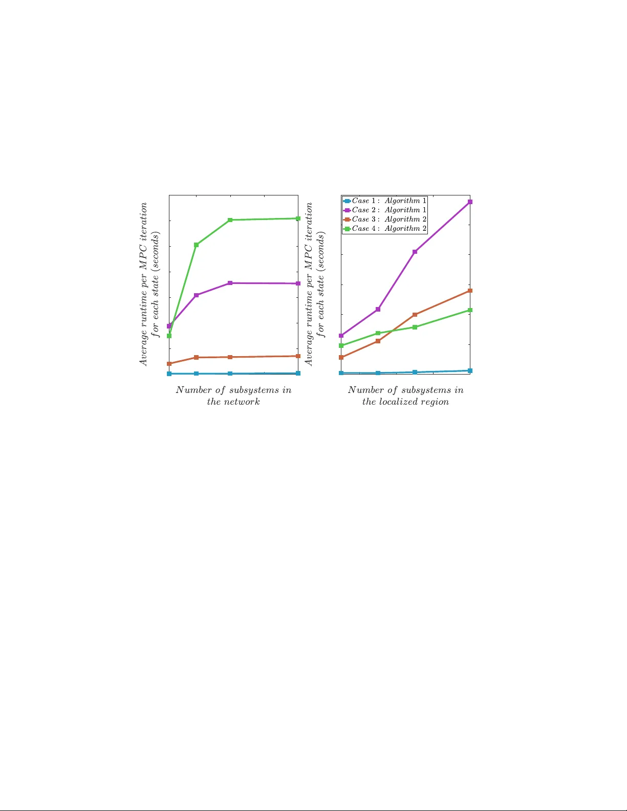
Distrib uted and Localized Closed Loop Model Pr edictiv e Contr ol via System Lev el Synthesis Carmen Amo Alonso ∗ Nikolai Matni † September 22, 2019, Re vised: September 14, 2020 Abstract W e present the Distributed and Localized Model Predicti ve Control (DLMPC) algorithm for large- scale structured linear systems, a distributed closed loop model predictiv e control scheme wherein only local state and model information needs to be exchanged between subsystems for the computation and implementation of control actions. W e use the System Le vel Synthesis (SLS) frame work to reformulate the centralized MPC problem as an optimization problem over closed loop system responses, and sho w that this allows us to naturally impose localized communication constraints between sub-controllers. W e show that the structure of the resulting optimization problem can be exploited to dev elop an Alternating Direction Method of Multipliers (ADMM) based algorithm that allows for distributed and localized computation of distributed closed loop control policies. W e conclude with numerical simulations to demonstrate the usefulness of our method, in which we sho w that the computational comple xity of the subproblems solved by each subsystem in DLMPC is independent of the size of the global system. T o the best of our knowledge, DLMPC is the first MPC algorithm that allo ws for the scalable distributed computation of distributed closed loop control policies. 1 INTR ODUCTION Model Predictiv e Control (MPC) has seen widespread success across many applications. Ho wev er , the re- cent need to control increasingly large-scale, distrib uted, and networked systems has limited its applicability . Large-scale distrib uted systems are often impossible to control with a centralized controller , and moreover , e ven when such a centralized controller can be implemented, the high computational demand of MPC ren- ders it impractical. Thus, efforts ha v e been made to dev elop distributed MPC (DMPC) algorithms, wherein sub-controllers solve a local optimization problem, and potentially coordinate with other sub-controllers. The majority of DMPC research has focused on open-loop approaches, which, follo wing the discussion in [1], can be broadly categorized into non-cooperativ e and cooperative settings. In the non-cooperativ e setting (see for example [2]), sub-controllers do not coordinate their actions with each other , and treat other subsystems as disturbances: while computationally ef ficient, such approaches are known to be conservati v e, and can e v en lead to infeasible problems, when there is strong dynamic coupling between subsystems. In the cooperati ve setting, sub-controllers exchange state and control action information in order to coordinate their behavior so as to optimize a global objectiv e, typically through distributed optimization: see for example [1, 3 – 8]. In order to make these nominal open loop approaches robust to additiv e disturbances, two broad approaches hav e been taken to generate closed loop policies. ∗ C. Amo Alonso is a graduate student in the Computing and Mathematical Sciences Department at California Institute of T echnology , Pasadena, CA. camoalon@caltech.edu † N. Matni is an Assistant Professor with the Department of Electrical and Systems Engineering at the University of Pennsylv a- nia, Philadelphia, P A. nmatni@seas.upenn.edu The first extends centralized robust MPC techniques that rely on a pre-computed stabilizing controller , such as constraint tightening and tube MPC, to the distributed setting. While conceptually appealing and computationally ef ficient, they often rely on strong assumptions, such as the existence of a static structur ed stabilizing controller , as in [9], which can be NP-hard to compute [10], or on dynamically decoupled subsys- tems, as in [11]. The alternativ e approach, and that which is adopted in this paper , is to compute a dynamic structured feedback policy using a suitable parameterization. The first paper to propose such a strategy was the seminal paper by Goulart et al. [12], where it w as sho wn that using a disturbance based parameterization of the control policy allo wed for distributed (structured) control policies to be synthesized using con ve x opti- mization. A similar approach exploiting Quadratic In v ariance [13] and the Y oula parameterization was also recently dev eloped in [14]. While these methods allow for con ve x optimization to be used for the synthesis of distributed closed loop control policies, the resulting optimization problems lack the structure needed for them to be amenable to distributed optimization techniques, limiting their applicability to smaller scale systems. Thus, the desiderata for a closed loop DMPC algorithm are that it allo w for (i) structured feedback policies to be computed via conv ex optimization, and (ii) for this computation to be solvable at scale via distributed optimization techniques: to the best of our kno wledge, no method satisfying both requirement exists. In this paper we address this gap and present the Distributed Localized MPC (DLMPC) algorithm for linear time-in v ariant systems, which allo ws for the distributed computation of structured feedback policies. W e lev erage the System Lev el Synthesis [15 – 17] (SLS) framework to define a nov el parameterization of distributed closed loop MPC policies such that the resulting synthesis problem is both con vex and struc- tur ed , allowing for the natural use of distributed optimization techniques. W e show that by exploiting the sparsity of the underlying distributed system and resulting closed loop system, as well as the separability properties [16] of often used objective functions and constraints (e.g., quadratic costs subject to polytopic constraints), we are able to distribute the computation via the Alternating Direction Method of Multipliers (ADMM), thus allowing for the online computation of closed loop MPC policies to be done in a scalable localized manner . Hence, in the resulting implementation each sub-controller solves a lo w-dimensional op- timization problem defined ov er its local neighborhood, requiring only local communication of state and model information. W e show that so long as certain localizability properties are satisfied, no approxima- tions are needed, and that under standard regularity assumptions, the algorithm conv erges to the globally optimal solution. Furthermore, we show that con ve x constraints and cost functions that couple neighboring subsystems can be dealt with via a consensus-like algorithm. Through numerical experiments, we further confirm that the complexity of the subproblems solved at each subsystem scales as O (1) relati v e to the full size of the system. Notation Bracketed indices denote the time of the true system, i.e., x ( t ) denotes the system state at time t , subscripts denote prediction time indices within an MPC loop, i.e., x t denotes the t th predicted state, and superscripts denote iteration steps of an optimization algorithm, i.e., x k t is the value of the t th predicted state at iterate k . T o denote subsystem variables, we use square bracket notation, i.e., [ x ] i denotes the components of x corresponding to subsystem i . Calligraphic letters such as S denote sets, and lowercase script letters such as c denotes a subset of Z + , i.e., c = { 1 , ..., n } ⊂ Z + . Boldface lower and upper case letters such as x and K denote finite horizon signals and lo wer block triangular (causal) operators, respecti vely: x =      x 0 x 1 . . . x T      , K =      K 0 , 0 K 1 , 1 K 1 , 0 . . . . . . . . . K T ,T . . . K T , 1 K T , 0      , where each K i,j is a matrix of compatible dimension. K ( r , c ) denotes the submatrix of K composed of the ro ws specified by r and the columns specified by c . 2 PR OBLEM FORMULA TION Consider a discrete-time linear time in v ariant (L TI) system x ( t + 1) = Ax ( t ) + B u ( t ) + w ( t ) , (1) where x ( t ) ∈ R n is the state, u ( t ) ∈ R p is the control input, and w ( t ) ∈ R n is an exogenous disturbance. The system is composed of N interconnected subsystems, as defined by an interconnection topology – cor- respondingly , the state, control, and disturbance inputs can be suitably partitioned as [ x ] i , [ u ] i , and [ w ] i , inducing a compatible block structure [ A ] ij , [ B ] ij in the dynamics matrices ( A, B ) . W e model the intercon- nection topology of the system as a time-in variant 1 unweighted directed graph G ( A,B ) ( E , V ) , where each subsystem i is identified with a v ertex v i ∈ V and an edge e ij ∈ E exists whenev er [ A ] ij 6 = 0 or [ B ] ij 6 = 0 . Example 1. Consider the linear time-in variant system structur ed as a chain topology as shown in F igur e 1. Each subsystem i is subject to the dynamics [ x ( t + 1)] i = X j ∈{ i,i ± 1 } [ A ] ij [ x ( t )] j + [ B ] ii [ u ( t )] i + [ w ( t )] i . As B is a diagonal matrix, coupling between subsystems is defined by the A matrix – thus, the adjacency matrix of the corr esponding graph G coincides with the support of A . . . . . …. …. . . . . …. …. [ u ] j [ u ] i [ u ] 1 [ x ] 1 [ x ] i [ x ] j [ w ] 1 [ w ] i [ w ] j [ x ] j [ x ] i [ x ] 1 [ u ] N [ x ] N [ x ] N [ w ] N Figure 1: Schematic representation of a system with a chain topology . As is standard, a model predicti ve controller is implemented by solving a series of finite horizon optimal control problems, with the problem solved at time τ with initial condition x 0 = x ( τ ) over a prediction horizon T giv en by: min. x t ,u t ,γ t T − 1 X t =0 f t ( x t , u t ) + f T ( x T ) s.t. x 0 = x ( τ ) , x t +1 = Ax t + B u t , t = 0 , ..., T − 1 , x T ∈ X T , x t ∈ X t , u t ∈ U t t = 0 , ..., T − 1 , u t = γ t ( x 0: t , u 0: t − 1 ) , (2) 1 Although we restrict both the dynamics and interconnection topology to be time-inv ariant, we believ e that an e xtension to time- varying dynamics and topologies will be straightforw ard as long as the corresponding communication topology varies consistently with the physical topology . W e leave this e xtension for future work. where the f t ( · , · ) and f T ( · ) are conv ex cost functions, X t and U t are con ve x sets containing the origin, and γ t ( · ) are measurable functions of their ar guments. Our goal is to define a MPC algorithm that respects local communication constraints between sub- controllers, and has only local-scale computational complexity when computing and subsequently imple- menting distrib uted closed loop control policies. In what follo ws, we formally define appropriate notions of locality in terms of the interconnection topology graph G ( A,B ) of the underlying physical system, and relate these to the corresponding constraints that they impose on the MPC problem (2). W e assume that the information exchange topology between sub-controllers matches that of the under- lying system, i.e., that it is giv en by G ( A,B ) , and we further impose that information exchange be localized to a subset of neighboring sub-controllers. In particular , we use the notion of a d -local information exchange constraint [18, 19] to be one that restricts sub-controllers to exchange their state and control actions with neighbors at most d -hops aw ay , as measured by the communication topology G ( A,B ) . This notion is captured by the d -outgoing and d -incoming sets of subsystem. Definition 1. F or a graph G ( V , E ) , the d-outgoing set of subsystem i is out i ( d ) := { v j | dist ( v i → v j ) ≤ d ∈ N } . The d-incoming set of subsystem i is in i ( d ) := { v j | dist ( v j → v i ) ≤ d ∈ N } . Note that v i ∈ out i ( d ) ∩ in i ( d ) for all d ≥ 0 . Hence, we can enforce a d -local information exchange constraint on the distributed MPC problem (2) by imposing the constraint that each sub-controllers policy respects [ u t ] i = γ i,t  [ x 0: t ] j ∈ in i ( d ) , [ u 0: t − 1 ] j ∈ in i ( d ) , [ A ] j,k ∈ in i ( d ) , [ B ] j,k ∈ in i ( d ) }  , (3) for all t = 0 , . . . , T and i = 1 , . . . , N , where γ i,t is a measurable function of its arguments. In words, this says that the closed loop control policy at sub-controller i can be computed using only states, control actions, and system models collected from d -hop incoming neighbors of subsystem i in the communication topology G ( A,B ) . Example 2. Consider a system (1) composed of N = 6 scalar subsystems, with B = I 6 and A matrix with support r epr esented in F igur e 2(a). This induces the inter connection topology gr aph G ( A,B ) illustrated in F igur e 2(b). The d -incoming and d -outgoing sets can be directly read off fr om the interaction topology . F or example , for d = 1 , the 1 -hop incoming neighbors for subsystem 5 ar e subsystems 3 and 4 , hence in 5 (1) = { 3 , 4 , 5 } ; similarly , out 5 (1) = { 4 , 5 , 6 } . [ x ] 1 [ x ] 2 [ x ] 3 [ x ] 4 [ x ] 5 [ x ] 6 in 5 ( 1) AAAB+XicdVDLSgMxFM3UV62vUZdugkWomyHTasfuim5cVrAPaIchk2ba0MyDJFMoQ//EjQtF3Pon7vwbM20FFT0QOJxzLzn3+AlnUiH0YRTW1jc2t4rbpZ3dvf0D8/CoI+NUENomMY9Fz8eSchbRtmKK014iKA59Trv+5Cb3u1MqJIujezVLqBviUcQCRrDSkmeagxCrsR9kLJp7lxX73DPLyLLr1QZqQGTV6g2EHE1QFdUdB9oWWqAMVmh55vtgGJM0pJEiHEvZt1Gi3AwLxQin89IglTTBZIJHtK9phEMq3WyRfA7PtDKEQSz0ixRcqN83MhxKOQt9PZnnlL+9XPzL66cquHL1UUmqaESWHwUphyqGeQ1wyAQlis80wUQwnRWSMRaYKF1WSZfwdSn8n3Sqll2zqncX5eb1qo4iOAGnoAJs4IAmuAUt0AYETMEDeALPRmY8Gi/G63K0YKx2jsEPGG+fErmTTA== ou t 5 ( 1) AAAB+nicdVDNS8MwHE3n15xfnR69BIcwL6WtG9tx6MXjBPcBWylplm5haVOSVBl1f4oXD4p49S/x5n9juk1Q0Qchj/d+P/LygoRRqWz7wyisrW9sbhW3Szu7e/sHZvmwK3kqMOlgzrjoB0gSRmPSUVQx0k8EQVHASC+YXuZ+75YISXl8o2YJ8SI0jmlIMVJa8s3yMEJqEoQZT9Xcr1edM9+s2Fbdtl2nAW1L302nBnPFtd0adLSSowJWaPvm+3DEcRqRWGGGpBw4dqK8DAlFMSPz0jCVJEF4isZkoGmMIiK9bBF9Dk+1MoIhF/rECi7U7xsZiqScRYGezIPK314u/uUNUhU2vYzGSapIjJcPhSmDisO8BziigmDFZpogLKjOCvEECYSVbqukS/j6KfyfdF3LObfc61qldbGqowiOwQmoAgc0QAtcgTboAAzuwAN4As/GvfFovBivy9GCsdo5Aj9gvH0C1bCTuA== [ x ] 1 [ x ] 2 [ x ] 3 [ x ] 4 [ x ] 5 in 5 ( 1) AAAB+XicdVDLSgMxFM3UV62vUZdugkWomyHTasfuim5cVrAPaIchk2ba0MyDJFMoQ//EjQtF3Pon7vwbM20FFT0QOJxzLzn3+AlnUiH0YRTW1jc2t4rbpZ3dvf0D8/CoI+NUENomMY9Fz8eSchbRtmKK014iKA59Trv+5Cb3u1MqJIujezVLqBviUcQCRrDSkmeagxCrsR9kLJp7lxX73DPLyLLr1QZqQGTV6g2EHE1QFdUdB9oWWqAMVmh55vtgGJM0pJEiHEvZt1Gi3AwLxQin89IglTTBZIJHtK9phEMq3WyRfA7PtDKEQSz0ixRcqN83MhxKOQt9PZnnlL+9XPzL66cquHL1UUmqaESWHwUphyqGeQ1wyAQlis80wUQwnRWSMRaYKF1WSZfwdSn8n3Sqll2zqncX5eb1qo4iOAGnoAJs4IAmuAUt0AYETMEDeALPRmY8Gi/G63K0YKx2jsEPGG+fErmTTA== ou t 5 ( 1) AAAB+nicdVDNS8MwHE3n15xfnR69BIcwL6WtG9tx6MXjBPcBWylplm5haVOSVBl1f4oXD4p49S/x5n9juk1Q0Qchj/d+P/LygoRRqWz7wyisrW9sbhW3Szu7e/sHZvmwK3kqMOlgzrjoB0gSRmPSUVQx0k8EQVHASC+YXuZ+75YISXl8o2YJ8SI0jmlIMVJa8s3yMEJqEoQZT9Xcr1edM9+s2Fbdtl2nAW1L302nBnPFtd0adLSSowJWaPvm+3DEcRqRWGGGpBw4dqK8DAlFMSPz0jCVJEF4isZkoGmMIiK9bBF9Dk+1MoIhF/rECi7U7xsZiqScRYGezIPK314u/uUNUhU2vYzGSapIjJcPhSmDisO8BziigmDFZpogLKjOCvEECYSVbqukS/j6KfyfdF3LObfc61qldbGqowiOwQmoAgc0QAtcgTboAAzuwAN4As/GvfFovBivy9GCsdo5Aj9gvH0C1bCTuA== G ( E, V ) AAAB+HicbVDLSgMxFL1TX7U+OurSTbAIFaTMVEGXRRFdVrAPaIeSSdM2NJMZkoxQh36JGxeKuPVT3Pk3ZtpZaOuBwOGce7knx484U9pxvq3cyura+kZ+s7C1vbNbtPf2myqMJaENEvJQtn2sKGeCNjTTnLYjSXHgc9ryx9ep33qkUrFQPOhJRL0ADwUbMIK1kXp2sRtgPSKYo9vyzWnzpGeXnIozA1ombkZKkKHes7+6/ZDEARWacKxUx3Ui7SVYakY4nRa6saIRJmM8pB1DBQ6o8pJZ8Ck6NkofDUJpntBopv7eSHCg1CTwzWQaUy16qfif14n14NJLmIhiTQWZHxrEHOkQpS2gPpOUaD4xBBPJTFZERlhiok1XBVOCu/jlZdKsVtyzSvX+vFS7yurIwyEcQRlcuIAa3EEdGkAghmd4hTfryXqx3q2P+WjOynYO4A+szx/3RZH6 supp( A )= 2 6 6 4 ? 00000 ?? 0000 ? 0 ? 000 0 ? 0 ?? 0 00 ??? 0 0000 ?? 3 7 7 5 AAADW3icjZLPb9MwFMedZGwl7EcH4sTFWrVpu1TJhsQuSAMuHIdEt0lNVTnua2fVcTz7ZaJE/Sc5bQf+FYTTFgRtxvhKlr56733s5OmbaiksRtG95wdrT9Y3Gk/DZ5tb2zvN3ecXNi8Mhw7PZW6uUmZBCgUdFCjhShtgWSrhMh1/qPqXt2CsyNVnnGjoZWykxFBwhq7U3/VuQuqUZAyvTVbaQuvp4bsj+pYmlhuh0YqvMB9JYSRUmbpJI75MXR+ZoQc0WjlJMgOW9QuoBx+BolrwAWh5ePXlf4B1wH+D9RckoAa/Fxf2m62oHc1EV028MC2y0Hm/+S0Z5LzIQCGXzNpuHGnslcyg4BKmYVJY0IyP2Qi6ziqWge2Vs2xM6b6rDOgwN+4opLPqn0TJMmsnWeomqwzY5V5VrOt1Cxye9kqhdIGg+PyhYSEp5rQKGh0IAxzlxBnmkuS+lfJrZhhHF8dqCfHyL6+ai+N2fNI+/vS6dfZ+sY4GeUX2yCGJyRtyRj6Sc9Ih3LvzfvgbfsP/HgRBGGzOR31vwbwgfyl4+ROWHuAP [ x ] 1 [ x ] 2 [ x ] 3 [ x ] 4 [ x ] 5 [ x ] 6 in 5 (1) AAAB+XicdVDLSgMxFM3UV62vUZdugkWomyHTasfuim5cVrAPaIchk2ba0MyDJFMoQ//EjQtF3Pon7vwbM20FFT0QOJxzLzn3+AlnUiH0YRTW1jc2t4rbpZ3dvf0D8/CoI+NUENomMY9Fz8eSchbRtmKK014iKA59Trv+5Cb3u1MqJIujezVLqBviUcQCRrDSkmeagxCrsR9kLJp7lxX73DPLyLLr1QZqQGTV6g2EHE1QFdUdB9oWWqAMVmh55vtgGJM0pJEiHEvZt1Gi3AwLxQin89IglTTBZIJHtK9phEMq3WyRfA7PtDKEQSz0ixRcqN83MhxKOQt9PZnnlL+9XPzL66cquHL1UUmqaESWHwUphyqGeQ1wyAQlis80wUQwnRWSMRaYKF1WSZfwdSn8n3Sqll2zqncX5eb1qo4iOAGnoAJs4IAmuAUt0AYETMEDeALPRmY8Gi/G63K0YKx2jsEPGG+fErmTTA== out 5 (1) AAAB+nicdVDNS8MwHE3n15xfnR69BIcwL6WtG9tx6MXjBPcBWylplm5haVOSVBl1f4oXD4p49S/x5n9juk1Q0Qchj/d+P/LygoRRqWz7wyisrW9sbhW3Szu7e/sHZvmwK3kqMOlgzrjoB0gSRmPSUVQx0k8EQVHASC+YXuZ+75YISXl8o2YJ8SI0jmlIMVJa8s3yMEJqEoQZT9Xcr1edM9+s2Fbdtl2nAW1L302nBnPFtd0adLSSowJWaPvm+3DEcRqRWGGGpBw4dqK8DAlFMSPz0jCVJEF4isZkoGmMIiK9bBF9Dk+1MoIhF/rECi7U7xsZiqScRYGezIPK314u/uUNUhU2vYzGSapIjJcPhSmDisO8BziigmDFZpogLKjOCvEECYSVbqukS/j6KfyfdF3LObfc61qldbGqowiOwQmoAgc0QAtcgTboAAzuwAN4As/GvfFovBivy9GCsdo5Aj9gvH0C1bCTuA== G ( E, V ) AAAB+HicbVDLSgMxFL1TX7U+OurSTbAIFaTMVEGXRRFdVrAPaIeSSdM2NJMZkoxQh36JGxeKuPVT3Pk3ZtpZaOuBwOGce7knx484U9pxvq3cyura+kZ+s7C1vbNbtPf2myqMJaENEvJQtn2sKGeCNjTTnLYjSXHgc9ryx9ep33qkUrFQPOhJRL0ADwUbMIK1kXp2sRtgPSKYo9vyzWnzpGeXnIozA1ombkZKkKHes7+6/ZDEARWacKxUx3Ui7SVYakY4nRa6saIRJmM8pB1DBQ6o8pJZ8Ck6NkofDUJpntBopv7eSHCg1CTwzWQaUy16qfif14n14NJLmIhiTQWZHxrEHOkQpS2gPpOUaD4xBBPJTFZERlhiok1XBVOCu/jlZdKsVtyzSvX+vFS7yurIwyEcQRlcuIAa3EEdGkAghmd4hTfryXqx3q2P+WjOynYO4A+szx/3RZH6 (a) (b) Figure 2: (a) Support of matrix A . (b) Example of 1 -incoming and 1 -outgoing sets for subsystem 5 . Gi ven such an interconnection topology , it would be desirable to be able to specify that both the synthesis and implementation of a control action at each subsystem be localized, i.e., depend only on state, control action, and plant model information from d -hop neighbors, where the size of the local neighborhood d is a design parameter . W e will show that, structural compatibility assumptions between the cost function, state and input constraints, and information exchange constraints, DLMPC allows for precisely this by imposing appropriate d -local structural constraints on the closed loop system r esponses of the system. W e will make clear that the localized region parameter d allo ws for a principled trade-of f between the amount of coordination allowed between sub-controllers and the computational complexity of the distributed MPC controller . T o do so, we le verage the SLS frame work to reformulate the MPC problem (2). 3 SYSTEM LEVEL SYNTHESIS B ASED DLMPC W e first introduce relev ant tools from the SLS framework[15 – 17], and show ho w SLS naturally allo ws for locality constraints [16, 18, 19] to be imposed on the system responses and corresponding controller implementation. 3.1 Time Domain System Le vel Synthesis The following is adapted from § 2 of [17]. Consider the dynamics of system (1) ev olving o ver a finite horizon t = 0 , ...T , and let u t be a causal linear time-varying state-feedback controller , i.e., u t = K t ( x 0 , x 1 , ..., x t ) where K t is some linear map to be designed. 2 Let Z be the block-do wnshift matrix, i.e., a matrix with iden- tity matrices along its first block sub-diagonal and zeros elsewhere, and define ˆ A := blkdiag( A, A, ..., A, 0) and ˆ B := blkdiag ( B , B , ..., B , 0) . This allo ws us to write the behavior of system (1) over the horizon t = 0 , ..., T as x = Z ( ˆ A + ˆ B K ) x + w , (4) where x , u and w are the finite horizon signals corresponding to state, control input, and disturbance re- specti vely . In particular , the initial condition x 0 is embedded as the first element of the disturbance, i.e., w = [ x T 0 w T 0 . . . w T T − 1 ] T . The closed loop behavior of system (1) under the feedback law K can be entirely characterized by the system responses Φ x and Φ u x = ( I − Z ( ˆ A + ˆ B K )) − 1 w =: Φ x w u = K ( I − Z ( ˆ A + ˆ B K )) − 1 w =: Φ u w . (5) The approach taken by SLS is to directly parameterize and optimize ov er the set of achiev able closed loop maps (5) from the exogenous disturbance w to the state x and the control input u , respectiv ely . Theorem 1. F or the dynamics (1) evolving under the state-feedback policy u = Kx , for K a block-lower - triangular matrix, the following ar e true 1. The affine subspace of bloc k lower -triangular { Φ x , Φ u } h I − Z ˆ A − Z ˆ B i  Φ x Φ u  = I (6) parameterizes all possible system r esponses (5) . 2. F or any block-lower -triangular matrices { Φ x , Φ u } satisfying (6), the contr oller K = Φ u Φ − 1 x achie ves the desir ed r esponse (5) fr om w 7→ ( x , u ) . Pr oof. See Theorem 2.1 of [17]. 2 Our assumption of a linear policy is without loss of generality , as an affine control policy u t = K t ( x 0: t ) + v t can always be written as a linear policy acting on the homogenized state ˜ x = [ x ; 1] . Theorem 1 allows us to reformulate an optimal control problem ov er state and input pairs ( x , u ) as an equiv alent one over system responses { Φ x , Φ u } – a detailed description of how to do this for sev eral standard control problems is provided in § 2 of [17]. For the MPC subproblem (2), as no driving noise is present, we only hav e to account for the system response to the initial condition x 0 , i.e., w = [ x T 0 , 0 , ..., 0] T . Hence, by equation (5), x = Φ x [0] x 0 and u = Φ u [0] x 0 , where Φ x [0] and Φ u [0] denote the first block column of the block lower triangular response matrices Φ x and Φ u – in the sequel, we will sometimes abuse notation and write Φ x [0] = Φ x , Φ u [0] = Φ u , as in the absence of driving noise, only the first block columns of Φ x , Φ u need to be computed. W e can rewrite the MPC subproblem (2) as min Φ x , Φ u f ( Φ x x 0 , Φ u x 0 ) s.t. Z AB Φ = I , x 0 = x ( t ) , Φ x x 0 ∈ X T , Φ u x 0 ∈ U T , (7) where we use Z AB Φ = I to compactly denote constraint (6), X T := ⊗ T − 1 t =0 X t ⊗ X T , and similarly for U T , and f is suitably defined such that it is consistent with the objectiv e function of problem (2). T o see why optimization problem (7) is equiv alent to the original MPC problem (2), it suf fices to no- tice that for the noise free setting we consider in this paper , for a fixed initial condition x 0 any control sequence u ( x 0 ) := [ u > 0 , . . . , u > T − 1 ] > can be achie ved by a suitable choice of feedback matrix K ( x 0 ) such that u ( x 0 ) = K ( x 0 )[0] x 0 (that such a matrix always exists follo ws from a simple dimension counting argu- ment). As this control action can be achieved by a linear-time-v arying controller K ( x 0 ) , Theorem 1 states that there exists a corresponding achiev able system response pair { Φ x , Φ u } such that u ( x 0 ) = Φ u [0] x 0 . This is simply a restatement in the SLS parameterization of the well known fact that L TV controllers are as expressi v e as nonlinear controllers over a finite horizon, giv en a fixed initial condition and noise realization (which in this case is set to zero). Thus the SLS reformulation introduces no conservatism relativ e to open- loop MPC in the nominal (disturbance free) setting. W e defer discussion of the closed loop setting to the end of this section, where we show that the disturbance based parametrization [12] is as a special case of ours. Why use SLS f or Distrib uted MPC: In the centralized setting, where both the system matrices ( A, B ) and the system responses { Φ x , Φ u } are dense, the SLS parameterized problem (7) is slightly more com- putationally costly than the original MPC problem (2), as there are now n ( n + p ) T decision variables, as opposed to ( n + p ) T decision variables. Howe ver , under suitable localized structural assumptions on the objecti ve functions f t and constraint sets X T and U T , that by lifting to this higher dimensional parameteri- zation, the structure of the underlying system - as captured by the interconnection topology G ( A,B ) - can be fully e xploited. In particular , the interplay of the high dimensional parametrization and the system structure allo ws for not only the con ve x synthesis of a distributed closed loop control policy (as is similarly done in [12, 14]), but also for the solution of this conv ex synthesis problem to be computed using distributed optimization. This latter feature is one of our main contrib utions, and in particular , we show that the resulting number of optimization variables in the local subproblems solved at each sub-system scales as O ( d 2 T ) , and hence is independent of the global system size. T o the best of our knowledge, this is the first distributed closed loop MPC algorithm that enjoys such properties. 3.2 Locality in System Lev el Synthesis W e begin by commenting on controller implementation. Gi ven a pair of achie vable system responses { Φ x , Φ u } satisfying the af fine constraint (6), the control law achieving the desired system behavior can be implemented as u = Φ u ˆ w , ˆ x = ( Φ x − I ) ˆ w , ˆ w = x − ˆ x , (8) where ˆ x can be interpreted as a nominal state trajectory , and ˆ w = Z w is a delayed reconstruction of the disturbance. Note that Φ x − I is strictly lower block triangular (i.e., strictly causal), and thus the implementation defined in (8) is well posed [17]. W e further note that in the simplifi ed setting of no dri ving noise, this implementation reduces to u = Φ u [0] x 0 . The advantage of this controller implementation, as opposed to u = Φ u Φ − 1 x x , is that any structure imposed on the maps { Φ u , Φ x } translates directly to structure on controller implementation (8), naturally allowing for information exchange constraints to be imposed by imposing suitable sparsity structure on the responses { Φ x , Φ u } . W e now show that imposing d -local structure on the system responses, coupled with an assumption of compatible d -local structure on the objectiv e functions and constraints of the MPC problem (2), leads to a structur ed SLS MPC optimization problem (7). W e then dev elop an ADMM based distributed solution to this problem in Section 4. W e emphasize that while the results of [12, 14] allow for similar structural constraints to be imposed on the controller realization through the use of either disturbance feedback or Y oula parameterizations (subject to Quadratic In v ariance [13] conditions), the resulting synthesis problems do not enjoy the structure needed for distributed optimization techniques to be effecti v e, thus limiting their usefulness to smaller scale examples where centralized computation of policies is feasible. W e return to argue this point more formally at the end of this section, after introducing the necessary concepts. W e begin by defining the notion of d -localized system responses, which follo ws naturally from the notion of d -local information exchange constraints. They consist of system responses with suitable sparsity patterns such that the information exchange needed between subsystems to implement the controller realization (8) is limited to d -hop incoming and outgoing neighbors, as defined by the topology G ( A,B ) . Definition 2. Let [ Φ x ] ij be the submatrix of system r esponse Φ x describing the map fr om disturbance [ w ] j to the state [ x ] i of subsystem i . The map Φ x is d-localized if and only if for every subsystem j , [ Φ x ] ij = 0 ∀ i 6∈ out j ( d ) . The definition for d-localized Φ u is analogous b ut with perturbations to contr ol action [ u ] i at subsystem i . It follows immediately from the controller implementation (8) that if the system responses are d -localized, then so is the controller implementation. In particular , by enforcing d -localized structure on Φ x , only a cor- responding local subset [ ˆ w ] j ∈ in i ( d ) of ˆ w are necessary for subsystem i to compute its local disturbance estimate [ ˆ w ] i , which ultimately means that only local communication is required to reconstruct the rele v ant disturbances for each subsystem. Similarly , if d -localized structure is imposed on Φ u , then only a local subset [ ˆ w ] j ∈ in i ( d ) of the estimated disturbances [ ˆ w ] is needed for each subsystem to compute its control action [ u ] i . Hence, each subsystem only needs to collect information from its d -incoming set to implement the control law defined by (8), and similarly , only needs to share information with its d -outgoing set to allo w for other subsystems to implement their respectiv e control laws. Furthermore, such locality constraints are transparently enforced as additional subspace constraints in the SLS formulation (7). Definition 3. A subspace L d enfor ces a d -locality constr aint if Φ x , Φ u ∈ L d implies that Φ x is d -localized and Φ u is ( d + 1) -localized 3 . A system ( A, B ) is then d -localizable if the intersection of L d with the affine space of achie vable system r esponses (6) is non-empty 4 . Although d -locality constraints are always con v ex subspace constraints, not all systems are d -localizable. As we describe in Section 4, the locality diameter d can be viewed as a design parameter , and for the re- mainder of the paper , we assume that there exists a d << N such that the system ( A, B ) to be controlled is d -localizable. W e emphasize two facts. W e emphasize two facts. First, the parameter d is tuned inde- pendently of the horizon T , and captures how “far” in the interconnection topology a disturbance striking a 3 Notice that we are imposing Φ u to be ( d + 1) -localized because in order to localize the effects of a disturbance within the region of size d , the “boundary” controllers at distance d + 1 must take action (for more details the reader is referred to [17]). 4 This can be interpreted as a spatio-temporal generalization of controllability . Interested readers are referred to [15, 20], where the analogy is made formal. subsystem is allo wed to spread – as described in detail in [15, 18, 19], localized control can be thought of as a spatio-temporal generalization of deadbeat control. Second, although beyond the scope of this paper , all of the presented results e xtend naturally to systems that are approximately localizable using a robust v ariant of the SLS parameterization described in [17, 21]. Example 3. Consider the chain in Example 1, and suppose that we enfor ce a 1 -locality constraint on the system responses: then Φ x is 1 -localized and Φ u is 2 -localized. Due to the chain topology , this is equivalent to enfor cing a tridiagonal structure on Φ x and a pentadiagonal structure on Φ u . The r esult- ing 1 -outgoing and 2 -incoming sets at node i ar e then given by out i (1) = { i − 1 , i, i + 1 } and in i (2) = { i − 2 , i − 1 , i, i + 1 , i + 2 } , as illustrated in F igure 3. . . . . …. …. . . . . …. …. [ w ] 1 [ u ] N [ x ] N [ x ] N . . . . [ u ] 1 [ x ] 1 [ x ] 1 [ x ] 2 [ x ] 3 [ x ] 4 [ x ] 2 [ x ] 4 [ x ] 3 [ u ] 2 [ u ] 3 [ u ] 4 Localized region for [ w ] 1 Affected States Activated Subontrollers Figure 3: Graphical representation of the scenario described in Example 3. Finally , we introduce the necessary compatibility assumptions between the cost functions, state and input constraints, and d -local information exchange constraints. Assumption 1. The objective function f t in formulation (2) is such that f t ( x ) = P f t i ([ x ] j ∈ in i ( d ) , [ u ] j ∈ in i ( d ) ) . The constrain sets in formulation (2) ar e such that x ∈ X = X 1 × ... × X n , wher e x ∈ X if and only if [ x ] j ∈ in i ( d ) ∈ X i for all i , and idem for U . Assumption 1 imposes that whenever two subsystems are coupled through either the constraints or the objectiv e function, they then must be within the d -local regions, as defined by their corresponding d - incoming and d -outgoing sets, of one another . This is a natural assumption for large structured networks where couplings between subsystems tend to occur at a local scale. W e can formulate the DLMPC subproblem by incorporating locality constraints into the SLS MPC subproblem (7). min Φ x , Φ u P N i =1 f i ([ Φ x x 0 ] j ∈ in i ( d ) , [ Φ u x 0 ] j ∈ in i ( d ) ) s.t. [ Φ x x 0 ] j ∈ in i ( d ) ∈ X i , [ Φ u x 0 ] j ∈ in i ( d ) ∈ U i , i = 1 , . . . , N , Z AB Φ = I , x 0 = x ( t ) , Φ x , Φ u ∈ L d , (9) where the f i are defined so as to be compatible with the decomposition defined in Assumption 1. While it was not obvious how to impose locality constraints on information exchange in the original formulation of the MPC subproblem (2), it is straightforward to do so via the locality constraints Φ x , Φ u ∈ L d in formulation (9). As these locality constraints are defined in terms of the d -hop incoming and outgoing sets of the interconnection topology of the system G ( A,B ) , the structure imposed on the system responses { Φ u , Φ x } will be compatible with the structure of the matrix Z AB defining the affine constraint (6). This structural compatibility in all optimization variables, cost functions, and constraints is the key feature that we exploit to apply distributed optimization techniques in the next section to scalably and exactly solve problem (9). Remark 1. Note that although d -locality constraints can always be imposed as con vex subspace constraints, not all systems are d -localizable. As we describe in the sequel, the locality diameter d can be viewed as design parameter , and for the remainder of the paper , we assume that ther e exists a d << N such that the system ( A, B ) to be contr olled is d -localizable. Although be yond the scope of this paper , all of the pr esented r esults e xtend naturally to systems that ar e appr oximately localizable using a r obust variant of the SLS parameterization described in [17, 21]. W e end by commenting briefly as to why pre vious methods [12, 14] do not enjoy this feature. W e focus on the method defined in [12], as a similar argument applies to the synthesis problem in [14]. Intuiti v ely , the disturbance based feedback parameterization of [12] only parameterizes the closed loop map Φ u from w → u , and leaves the state x as a free variable. This can be made explicit by noticing that the distur- bance feedback parameterization of [12] can be recovered from the SLS parameterization of Theorem 1 by multiplying the affine constraint (6) by w on the right, and setting x = Φ x w . Further, this immediately implies, by the result of [19], that the SLS MPC subproblem (7) is equi v alent to the affine problem (9) when restricted to solving ov er linear-time-v arying feedback policies. Setting w = [ x > 0 , 0 , . . . , 0] > , and relabeling the corresponding decision v ariables in the SLS MPC subproblem (7) yields min x , Φ u f ( x , Φ u [0] x 0 ) s.t. ( I − Z ˆ A ) x = Z ˆ B Φ u [0] x 0 + E 1 x 0 , x 0 = x ( t ) , x ∈ X T , Φ u [0] x 0 ∈ U T , (10) where E 1 is a block-column matrix with first block element set to identity , and all others set to 0. This is a special case of the optimization problem over disturbance feedback policies suggested in Section 4 of [12] with only a nonzero initial condition. Notice that regardless as to what structure is imposed on the objecti ve functions, constraints, and the map Φ u , the resulting optimization problem is strongly and globally coupled by the af fine constraint ( I − Z ˆ A ) x = Z ˆ B Φ u x 0 + E 1 x 0 , because the state variable x is alw ays dense. A similar coupling arises in the Y oula based parameterization suggested in [14]. In contrast, by explicitly parameterizing the additional system response Φ x from process noise to state, i.e., from w → x , we can naturally enforce the structure needed for distributed optimization techniques to be fruitfully applied. 4 An ADMM based Distrib uted AND Localized Solution W e start with a brief ov erview of the ADMM algorithm, and then show ho w it can be used to decompose the DLMPC sub-problem (9) into sub-problems that can be solved using only d -local information. For the sake of clarity , we introduce a simpler version of the algorithm first where only dynamical coupling is considered, which we then extend to the constraints and objecti ve functions that introduce d -localized couplings, as defined in Assumption 1. 4.1 The Alternating Dir ection Method of Multipliers The ADMM [22] algorithm has proved successful solving large-scale optimization problems that respect a certain partial-separability structure. In particular , giv en the follo wing optimization problem min x,y f ( x ) + g ( y ) s.t. Ax + B y = c, (11) ADMM - in its scaled form - solves (11) with the follo wing update rules: x k +1 = arg min x f ( x ) + ρ 2    Ax + B y k − c + z k    2 2 y k +1 = arg min y g ( y ) + ρ 2    Ax k +1 + B y − c + z k    2 2 z k +1 = z k + Ax k +1 + B y k +1 − c. (12) ADMM is particularly powerful when the iterate sub-problems defined in equation (12) can be solved in closed form, which is the case in many practically relev ant cases [22], as this allows for rapid execution and con ver gence of the algorithm. Further , under mild assumptions ADMM enjoys strong and general con v ergence guarantees. Theorem 2. Assume that extended r eal valued functions f : R n → R ∪ { + ∞} and g : R m → R ∪ { + ∞} ar e closed, pr oper , and con vex. Moreo ver , assume that the unaugmented Lagrangian has a saddle point. Then, the ADMM iterates in equation (12) satisfy the following: • Residual con vergence: r t → 0 as t → ∞ , i.e. the iterates appr oach feasibility . • Objective con vergence: f ( x t ) + g ( z t ) → p ∗ as t → 0 , i.e. the objective function of the iterates appr oac hes the optimal value. • Dual variable con vergence: y t → y ∗ as t → ∞ , where y ∗ is a dual optimal point. Hence, we impose the following additional assumptions so as to ensure that Theorem 2 is applicable to the considered problem. Assumption 2. Pr oblem (9) has a feasible solution in the relative interior of X T and U T . Assumption 3. The constraint sets X T and U T in formulation (9) are closed and con ve x. The objective function f ( Φ x 0 ) is a closed, pr oper , and con ve x function for all choices of x 0 6 = 0 . 4.2 DLMPC algorithm No w we present the proposed algorithm for the localized synthesis of the DLMPC problem (9). 4.2.1 DLMPC without Coupling Constraints In this subsection we present here a simplified version of the algorithm that contains its main features: namely , we illustrate how to decompose the MPC subroutine (9) by exploiting its separability . W e begin by restricting ourselves to the case where neither the objectiv e function nor the constraints introduce any coupling between subsystems. In the next subsection the general version of the algorithm will be introduced. W e sho w that the DLMPC problem (9) can be decomposed into local subproblems that can be solved using only d -local information and system models. In particular , consider the DLMPC subproblem solv ed at time t : min Φ f ( Φ x 0 ) s.t. Z AB Φ = I , Φ x 0 ∈ P , Φ ∈ L d , x 0 = x ( t ) , (13) where we let Z AB := h I − Z ˆ A − Z ˆ B i , Φ := [ Φ T x Φ T u ] T , and Φ x 0 ∈ P ⇐ ⇒ Φ x x 0 ∈ X T and Φ u x 0 ∈ U T . Moreover , according to Assumption 1, f can be written as f ( x , u ) = P f i ([ x ] i , [ u ] i ) , or equi valently , that f ( Φ x 0 ) = P f i ( Φ ( r i , :) x 0 ) since  [ x ] i [ u ] i  = Φ ( r i , :) x 0 where r i is the set of rows in Φ corresponding to subsystem i . Similarly , the constraints must satisfy that x ∈ X = X 1 × ... × X n , where each [ x ] i ∈ X i , and idem for U , implying that Φ ( r i , :) x 0 ∈ P i . These notions are formalized through a slight modification of the definitions in [16]: Definition 4. The functional g ( Φ ) is column-wise separable with r espect to the partition c = { c 1 , ..., c p } if it can be written as g ( Φ ) = P p j =1 g j ( Φ (: , c j )) for some functionals g j for j = 1 , ..., p . Equivalently , g ( Φ ) is r ow-wise separ able with r espect to the partition r if it can be written as g ( Φ ) = P p j =1 g j ( Φ ( r j , :) . Definition 5. A constraint-set P is column-wise separ able with respect to the partition c = { c 1 , ..., c p } when Φ ∈ P ⇐ ⇒ Φ (: , c j ) ∈ P j for j = 1 , ..., p is satisfied for some sets P j for j = 1 , ..., p . Equivalently , P is r ow-wise separ able with r espect to the partition r if Φ ∈ P ⇐ ⇒ Φ ( r j , :) ∈ P j for j = 1 , ..., p . If all objectiv e functions and constraints in an optimization problem are column-wise (row-wise) sep- arable with respect to a partition c ( r ) of cardinality p , then the optimization problem trivially decomposes into p independent subproblems. Howe ver , while Assumption 1 imposes that f x 0 ( Φ ) = f ( Φ x 0 ) and P are row-wise separable in the optimization variable Φ , the achie vability constraint Z AB Φ = I is column- wise separable in the optimization v ariable Φ . As we show next, this partially-separable structure can be exploited within an ADMM based algorithm to reduce each ADMM iterate subproblem (12) to a ro w or column-wise separable optimization problem, allo wing the algorithm to decompose and be solved at scale. Definition 6. An optimization pr oblem is partially separable if it can be written as min Φ g ( r ) ( Φ ) + g ( c ) ( Φ ) s.t. Φ ∈ S ( r ) ∩ S ( c ) , (14) for r ow-wise separ able g ( r ) and S ( r ) , and column-wise separable g ( c ) and S ( c ) . Since problem (13) is partially separable, we reformulate the DLMPC subproblem (9) so that is of the form (14): min Φ , Ψ f ( Φ x 0 ) s.t. Z AB Ψ = I , Φ x 0 ∈ P , { Φ , Ψ } ∈ L d , Φ = Ψ . (15) By duplicating the decision variable, we can decompose the DLMPC subproblem (9) into a column-wise separable iterate subproblem in Φ , and a row-wise seperable iterate subproblem in Ψ – thus problem (15) is partially separable, and is amenable to a distributed solution via ADMM: Φ k +1 =    argmin Φ f ( Φ x 0 ) + ρ 2    Φ − Ψ k + Λ k    2 F s.t. Φ x 0 ∈ P , Φ ∈ L d    (16a) Ψ k +1 =    argmin Ψ    Φ k +1 − Ψ + Λ k    2 F s.t. Z AB Ψ = I , Ψ ∈ L d    (16b) Λ k +1 = Λ k + Φ k +1 − Ψ k +1 . (16c) The squared Frobenius norm is both ro w-wise and column-wise separable. Therefore, the resulting iterate subproblems in (16) are separable: iterate subproblem (16a) is ro w-wise separable with respect to the ro w partition r induced by the subsystem-wise partitions of the state and control inputs, [ x ] i and [ u ] i , iterate subproblem (16b) is column-wise separable with respect to the column partition induced in a analogous manner , and iterate subproblem (16c) is component-wise separable. Hence, each of the iterate subproblems in (16) can be decomposed into column, row , or element-wise subproblems that can solved independently and in parallel, with each sub-controller i computing the solution to its component of the row or column-wise partition. Moreov er , by enforcing that the system responses be d -localized, i.e., that Φ x , Φ u ∈ L d , the resulting subproblem variables are sparse, allowing for a significant reduction in the dimension of the local subprob- lem. For example, when considering the column-wise subproblem ev aluated at subsystem j , the i th ro w of the j th subsystem column partitions of Φ x (: , c j ) and Φ u (: , c j ) ) is nonzero only if i ∈ ∪ k ∈ out j ( d ) r k and i ∈ ∪ k ∈ out j ( d +1) r k , respecti vely . In particular , sub-controller i solves the subproblems: [ Φ ] k +1 i r =      argmin [ Φ ] i r f i ([ Φ ] i r [ x 0 ] i r ) + ρ 2    [ Φ ] i r − [ Ψ ] k i r + [ Λ ] k i r    2 F s.t. [ Φ ] i r [ x 0 ] i r ∈ P i      (17a) [ Ψ ] k +1 i c =      argmin [ Ψ ] i c    [ Φ ] k +1 i c − [ Ψ ] i c + [ Λ ] k i c    2 F s.t. [ Z AB ] i c [ Ψ ] i c = [ I ] i c      (17b) [ Λ ] k +1 i r = [ Λ ] k i r + [ Φ ] k +1 i r − [ Ψ ] k +1 i r , (17c) where to lighten notational burden, we let [ Φ ] i r := Φ ( s r i , r i ) , where the set r i represents the set of ro ws that the controller i is solving for , and the set s r i is the set of columns associated to the ro ws in r i by the locality constraints L d . An equiv alent argument applies to [ Φ ] i c := Φ ( c i , s c i ) where the set c i represents the set of columns that the controller i is solving for , and the corresponding set s c i is the set of columns associated to the rows in c i . For example, when considering the row-wise subproblem (17a) ev aluated at subsystem i , the j th column of the i th subsystem row partition Φ x ( r i , :) and Φ u ( r i , :) is nonzero only if j ∈ in j ( d ) and j ∈ in j ( d + 1) , respectiv ely . It follo ws that subsystem i only requires a corresponding subset of the local sub-matrices [ A ] k,` , [ B ] k,` to solve its respectiv e subproblem. All column/ro w/matrix subsets described abov e can be found algorithmically (see Appendix A of [16]). Remark 2. Pr oblem (17b) can be solved in closed form: [ Ψ ] k +1 i c =  [ Φ ] k +1 i c + [ Λ ] k i c  + [ Z AB ] + i c  [ I ] i c − [ Z AB ] i c  [ Φ ] k +1 i c + [ Λ ] k i c   , (18) wher e [ Z AB ] + i c denotes the pseudo-in verse of [ Z AB ] i c . This pseudo-in verse can be computed once off-line, r educing the evaluation of update step (18) to matrix multiplication. Notice that in general, in general r i ⊂ s c i and c i ⊂ s r i . Hence, each subsystem i is computing updates for the sub-matrix Φ ( s r i , c i ) and the sub-matrix Φ ( r i , s c i ) of the global system response v ariables Φ and Ψ . In particular, for subsystem i to solve its local iterate subproblems (17), information sharing among subsystems is needed. Howe ver , as we impose d -locality constraints on the system responses, information only needs to be collected from d-hop neighbors. Similarly , only a d -local subset initial condition x 0 = x ( t ) is needed to solve the local iterate subproblems (17). Algorithm 1 summarizes the implementation at subsystem i of the ADMM based solution to the DLMPC subproblem (9). In the final step of Algorithm 1, we let [ x 0 ] s r i denote the subset of elements of x 0 associated with the columns in s r i , such that [Φ 0 , 0 u ] i r x 0 = [Φ 0 , 0 u ] i r [ x 0 ] s r i 5 . Algorithm 1 is run in parallel by each sub- controller , and makes clear that only d -local information and system models are needed to solv e the ADMM 5 Recall that per in the notation section, Φ 0 , 0 u represents the upper-most left-most matrix in the block-diagonal operator Φ u . iterate subproblems (17) at subsystem i . Algorithm 1 Subsystem i DLMPC implementation 1: input: con ver gence tolerance parameters  p > 0 ,  d > 0 2: Measure local state [ x ( t )] i . 3: Share the measurement with out i ( d ) . 4: Solve optimization problem (17a). 5: Share [ Φ ] k +1 i r with out i ( d ) . Receiv e the corresponding [ Φ ] k +1 j r from in i ( d ) and build [ Φ ] k +1 i c . 6: Solve optimization problem (17b) via the closed form solution (18). 7: Share [ Ψ ] k +1 i c with out i ( d ) . Receiv e the corresponding [ Ψ ] k +1 j c from in i ( d ) and build [ Ψ ] k +1 i r . 8: Perform the multiplier update step (17c). 9: Check con v ergence as    [ Φ ] k +1 i r − [ Ψ ] k +1 i r    F ≤  p and    [ Ψ ] k +1 i r − [ Ψ ] k i r    F ≤  d . 10: If con ver ged, apply computed control action [ u 0 ] i = [Φ 0 , 0 u ] i r [ x 0 ] s r i , and return to 2, otherwise return to 4. Computational complexity of the algorithm The computational complexity of the algorithm is determined by update steps 4, 6 and 8. In particular , steps 6 and 8 can be directly solved in closed form, reducing their ev aluation to the multiplication of matrices of dimension O ( d 2 T ) . In certain cases, step 4 can also be computed in closed form if a proximal operator exists for the formulation. For instance this is true if it reduces to quadratic conv ex cost function subject to af fine equality constraints. Regardless, each local iterate sub-problem is ov er O ( d 2 T ) optimization v ariables subject to O ( dT ) constraints, leading to a significant computational saving when d << N . The commu- nication complexity - as determined by steps 3, 5 and 7 - is limited to the local exchange of information between d -local neighbors. Con ver gence of the algorithm One can sho w con ver gence by le veraging Theorem 2. Corollary 2.1. Algorithm 1 satisfies r esidual con ver gence, objective conver gence and dual variable con ver - gence as defined in Theor em 2. Pr oof. Algorithm 1 is built upon algorithm (17), which is merely algorithm (16) after exploiting locality . Thus to prov e Corollary 2.1 we only need to show that the ADMM algorithm (16) satisfies the assumptions in Theorem 2. Define the extended-real-v alue functional h ( Φ ) by h ( Φ ) = ( Φ x 0 if Z AB Φ = I , Φ x 0 ∈ P , Φ ∈ L d ∞ otherwise . The constrained optimization in (15) can equiv alently be written in terms of h ( Φ ) with the constraint Φ = Ψ . min Φ , Ψ h ( Φ ) s.t. Φ = Ψ . Notice that by Assumption 3, f ( Φ x 0 ) is closed, proper, and con ve x, and P is a closed and con ve x set. Moreov er , the remaining constraints Z AB Φ = I and Φ ∈ L d are also closed and con ve x. Hence, h ( Φ ) is closed, proper , and con ve x. It only remains to sho w that the Lagrangian has a saddle point. This condition is equiv alent to sho wing that strong duality holds [23]. By Assumption 2, Slater’ s condition is automatically satisfied, and therefore the Lagrangian of the problem has a saddle point. Since both conditions of Theorem 2 are satisfied, the ADMM algorithm in (16) satisfies residual con ver gence, objecti ve con v ergence and dual v ariable con ver gence as defined in Theorem 2. Since Algorithm 1 results from le veraging (16), guaranteeing con v ergence of algorithm (16) automatically guarantees con v ergence of Algorithm 1. Recursive feasibility and stability In order to guarantee recursi ve feasibility , we can make the standard assumption that the horizon N is chosen suf ficiently long (Corollary 13.2, [24]). As the complexity of the subproblems now scales with the localized radius d , choosing a longer horizon N no longer represents as substantial a computational burden. Similarly , in order to guarantee stability , a simple sufficient condition is to set the terminal constraint [ x N ] i = 0 . Al- though this is a conserv ativ e sufficient condition, and we lea ve exploring the development of more principled terminal costs and constraint sets as well as integrating robustness to additiv e disturbance to future work, the ability of SLS to synthesize localized distributed controllers that define localized forward in v ariant sets satisfying state and input constraints [25] via distributed optimization of fers a promising a venue forw ard. Communication dropouts In real-life applications, communication lost due to data losses or corrupted communications links can oc- cur . Given that the presented algorithm relies on multiple exchanges of information between the subsystems, ho w communication lost af fects the closed-loop performance of the algorithm is an interesting question. Al- though a formal analysis is left as future research, the work done in [26] illustrates that it w ould be possible to slightly modify the proposed ADMM-based scheme to make it robust to unreliable communication links. Furthermore, extensions of ADMM to deal with data pri v acy and leakage when agents exchange information such as the ones carried out in [27] can be directly applicable to our frame work for sensitiv e-data applica- tions. Lastly , the impact of the netw ork topology in the con ver gence and performance of ADMM as studied in [28] sets the ground for extending this w ork to time-changing topologies. 4.2.2 DLMPC subject to localized coupling constraints Building on Algorithm 1, we now show how DLMPC can be extended to allow for coupling between sub- systems by the constraints and objecti ve function, so long as the coupling is compatible with the d -localized constraints being imposed, i.e., so long as the objecti ve function and constraints satisfy Assumption 1. Con- sider the DLMPC sub-problem (13), where the objecti ve function and constraints satisfy the locality prop- erties imposed by Assumption 1. Due to this local coupling, the problem is no longer partially separable – ho wev er , we may still re write it as min X , Φ f ( X ) s.t. X = Φ x 0 , Z AB Φ = I X ∈ P , Φ ∈ L d . (19) The first constraint is row-wise separable for Φ while the second is column-wise separable in Φ . Ap- plying the same v ariable duplication process as abov e and applying ADMM yields [ Φ k +1 , X k +1 ] =      argmin Φ , X f ( X ) + ρ 2    Φ − Ψ k + Λ k    2 F s.t. X = Φ x 0 , X ∈ P , Φ ∈ L d      (20a) Ψ k +1 =    argmin Ψ    Φ k +1 − Ψ + Λ k    2 F s.t. Z AB Ψ = I , Ψ ∈ L d    (20b) Λ k +1 = Λ k + Φ k +1 − Ψ k +1 (20c) While the iterate sub-problems (20b) and (20c) enjoy column-wise and element-wise separability , iterate sub-problem (20a) is subject to local coupling due to the objective function f and constraint X ∈ P . In order to solve sub-problem iterate (20a) in a manner that respects the d -localized communication constraints, we propose an ADMM based consensus-like algorithm, similar to that used in [29]. Hence, the solution to iterate sub-problem (20a) is obtained by having each subsystem i solve [[ Φ ] k +1 ,n +1 i r , [ X ] n +1 i s ] =              argmin [ Φ ] i r , [ X ] i s f i ( X ) + ρ 2   [ Φ ] i r − [ Ψ ] n i r + [ Λ ] n i r   2 F + µ 2 X j ∈ in i ( d )    [ X ] n +1 j − [ Z ] i + [ Y ] n ij    2 F s.t. [ X ] i = [ Φ ] i r [ x 0 ] i r , [ X ] i s ∈ P i              (21a) [ Z ] n +1 i = 1 | in i ( d ) | X j ∈ in i ( d )    [ X ] n +1 j + [ Y ] n ij    2 F (21b) [ Y ] n +1 ij = [ Y ] n ij + [ X ] n +1 i − [ Z ] n +1 j , (21c) where the notation used is as in (17). In particular [ X ] i s is the concatenation of components [ X ] j satisfying j ∈ in i ( d ) , whereas [ X ] i is restricted to only those components of [ X ] i s needed by subsystem i to compute [ Φ ] i r x 0 = [ Φ ] i r [ x 0 ] s r i . After reaching consensus in equations (21), one can use [ Φ ] k +1 i r in algorithm (17). Therefore by solving iterate sub-problem (17a) using the ADMM based consensus-like updates (21), we are able to accommodate d -local coupling introduced in the constraints and objectiv e function while still only exchanging information with d -local neighbors. The rest of the analysis follows just as in the previous subsection. Algorithm 2 summarizes the general DLMPC algorithm as implemented at subsystem i . Remark 3. Notice that in pr oblem (21) each subsystem i optimizes for [ X ] i s , while in Algorithm 2 sub- systems only exchang e [ X ] i . This is standard in consensus algorithms wher e only the components of X corr esponding to subsystem i , [ X ] i needs to be exc hanged. Computational complexity and con ver gence guarantees The presence of the coupling inevitably results in an increase of the computation and communication com- plexity of the algorithm. The computational complexity of the algorithm is now determined by steps 4, 6, 8, 11 and 13. All of these except for step 4 can be solved in closed form. Once again, by Assumption 1 all sub-problems are over O ( d 2 T ) optimization variables and O ( dT ) constraints, so the complexity does not increase with the size of the netw ork. There is ho we ver an increased computational b urden due to the nested consensus-like algorithm used to solve iterate sub-problem (20a), which leads to an increase in the number Algorithm 2 Subsystem i implementation of DLMPC general subject to localized coupling 1: input: con ver gence tolerance parameters,  p ,  d ,  x > 0 . 2: Measure local state [ x 0 ] i . 3: Share measurement with out i ( d ) . 4: Solve optimization problem (21a). 5: Share [ X ] n +1 i with out i ( d ) . Receiv e the corresponding [ X ] n +1 j from in i ( d ) . 6: Perform update (21b). 7: Share [ Z ] n +1 i with out i ( d ) . Receiv e the corresponding [ Z ] n +1 j from in i ( d ) . 8: Perform update (21c). 9: If   [ X ] n +1 i − [ Z ] n +1 i   F <  x go to step 10, otherwise return to step 4. 10: Share [ Φ ] k +1 i r with out i ( d ) . Receiv e the corresponding [ Φ ] k +1 j r from in i ( d ) and build [ Φ ] k +1 i c . 11: Solve optimization problem (17b) via the closed form solution (18). 12: Share [ Ψ ] k +1 i c with out i ( d ) . Receiv e the corresponding [ Ψ ] k +1 j c from in i ( d ) and build [ Ψ ] k +1 i r . 13: Perform the multiplier update (17c). 14: Check con v ergence as    [ Φ ] k +1 i r − [ Ψ ] k +1 i r    F ≤  p and    [ Ψ ] k +1 i r − [ Ψ ] k i r    F ≤  d . 15: If conv erged, apply computed control action [ u 0 ] i = [Φ 0 , 0 u ] i r [ x 0 ] s r i , and return to step 2, otherwise return to step 4. of iterations needed for con v ergence. This also results in increased communication between subsystems, as local information exchange is needed as part of the consensus-like step as well. Ho wev er , once again this exchange is limited to within a d -local subset of the system, resulting in small consensus problems that con v erge quickly , as we illustrate empirically in the next section. Since Algorithm 2 is identical to Algorithm 1 save for the approach to solving the first iterate sub- problem, con v ergence follows from a similar argument as that used to prove Corollary 2.1. The same argument for recursi v e feasibility and stability expressed in the pre vious subsection holds for Algorithm 2. 5 SIMULA TION EXPERIMENTS In this section we illustrate the benefits of DLMPC as applied to large-scale distributed systems. T o do so, we consider two case-studies. In the first, we aim to illustrate how the proposed algorithm accounts for general con ve x coupling objectiv e functions and constraints. In the second, we empirically characterize the computational complexity properties of DLMPC. All code needed to replicate these experiments is a vailable at https://github.com/unstable- zeros/dl- mpc- sls . 5.1 Optimization features In this example we use a dynamical system consisting of a chain of four pendulums coupled through a spring ( 1 N /m ) and a damper ( 3 N s/m ). Each pendulum is modeled as a two-state subsystem described by its angle θ and angular v elocity ˙ θ . Each of the pendulums can actuate its v elocity . The simulations are done with a prediction horizon of T = 10 s , and we impose a localized region of size d = 1 subsystems. The initial condition is arbitrarily generated with MA TLAB rng(2020) . In order to illustrate ho w the presented algorithm can accommodate local coupling between subsystems as introduced by the objectiv e function and constraints, we begin with the following example. W e compare the control performance achie ved by solutions to the DLMPC sub-problem (13) computed as a centralized problem using the Gurobi solver [30] and CVX interpreter [31], [32] (dotted line), and using Algorithm 1 or 2 (solid line), as appropriate, in Figure 4. In particular , we plot the ev olution of the position of the first two pendulums under different control objectives and constraints. In scenario 1 we consider the quadratic cost f ( x , u ) = P 4 i =1 k [ x ] i k 2 2 + k [ u ] i k 2 2 , and hav e no additional constraints. In Scenario 2 we consider a quadratic cost coupling the angle of adjacent pendulums, i.e. the control objectiv e is a sum of functionals of the form f ([ θ ] i , [ u ] i ) = ([ θ ] i − 1 2 P [ θ ] j ) 2 + [ ˙ θ ] 2 i + [ u ] 2 i . Finally , Scenario 3 uses the same objectiv e function as Scenario 2 and further constrains the maximal allow able deviation between subsystem angles, i.e., | [ θ ] i − [ θ ] j | ≤ 0 . 05 , for all t > 2 . Once again, the centralized solution coincides with the solution achie ved by either Algorithm 1 or 2, again v alidating the optimality of the algorithms proposed. 0 10 20 30 40 50 -1 -0.5 0 0.5 1 Open loop dynamics 0 10 20 30 40 50 -1 -0.5 0 0.5 1 Scenario1 0 10 20 30 40 50 -1 -0.5 0 0.5 1 Scenario2 0 10 20 30 40 50 -1 -0.5 0 0.5 1 Scenario3 Figure 4: The ev olution of the position of the first two pendulums in open loop is shown in the top left figure, whereas the top right most figure shows the position of the first two pendulums under MPC control with a quadratic penalty on state and input, and no constraints (scenario 1). The bottom left figure sho ws the position of the first two pendulums when the performance objective couples the angle of adjacent pendulums (scenario 2). On the bottom right, the position of the first two pendulums when the performance objectiv e and the constraints couple adjacent pendulums (scenario 3). In order to further illustrate the impact of introducing a terminal constraint, we use Scenario 1 in Figure 4 and we simulate the closed loop dynamics with the DLMPC controller both with and without terminal constraint x T = 0 . As can be seen in Figure 5, the system with terminal constraint reaches steady state faster at the expense of a higher optimal cost, specially at short time horizons. In the two closed loop scenarios presented in Figure 5, we show both the control performance achiev ed by the solutions to the DLMPC subproblem (13) using Algorithm 1 and the solution to the standard MPC subproblem (2) computed as a centralized problem using the Gurobi solver [30] and CVX interpreter [31]. Again, in both cases the centralized solution coincides with the solution achiev ed by Algorithm 1, so the solution achiev ed by Algorithm 1 is optimal. 5.2 Per subsystem computational complexity Here we sho w how Algorithms 1 and 2 allo w DLMPC to be applied to lar ge-scale systems. Here, we let the subsystem dynamics be described by [ x ( t + 1)] i = [ A ] ii [ x ( t )] i + X j ∈ in i ( d ) [ A ] ij [ x ( t )] j + [ B ] ii [ u ( t )] i 3 4 5 6 7 8 9 10 0 1000 2000 3000 4000 5000 0 10 20 30 40 50 -1 -0.5 0 0.5 1 0 10 20 30 40 50 -1 -0.5 0 0.5 1 3 4 5 6 7 8 9 10 0 1000 2000 3000 4000 5000 0 10 20 30 40 50 -1 -0.5 0 0.5 1 0 10 20 30 40 50 -1 -0.5 0 0.5 1 Figure 5: On the top from left to right: ev olution of the position of the first two pendulums in open loop, with MPC control and no terminal constraint, and with MPC control with terminal constraint. Both cases under the quadratic cost f ( x , u ) = P 4 i =1 k [ x ] i k 2 2 + k [ u ] i k 2 2 and T = 10 . On the bottom, the cost of both MPC setups with and without terminal constraints. , where [ A ] ii =  1 0 . 1 − 0 . 3 0 . 7  , [ A ] ij =  0 0 0 . 1 0 . 1  , [ B ] ii =  0 0 . 1  . The MPC horizon is T = 5 . W e present four different scenarios that encompass different degrees of computational complexity of Algorithms 1 and 2: • Case 1: per subsystem separable quadratic cost and no constraints. • Case 2: per subsystem separable quadratic cost and per subsystem separable constraints. • Case 3: quadratic cost coupling d -local subsystems and no constraints. • Case 4: quadratic cost and polytopic constraints coupling d -local subsystems. The computational complexity of each of the cases is determined by (i) if the row-wise iteration sub- problem can be solved in closed form, and (ii) if Algorithm 1 or 2 is needed – we summarize these properties for the four cases described abov e in T able 1. Case Algorithm Computation of step 4 1 1 Closed form 2 1 Needs minimization solver 3 2 Closed form 4 2 Needs minimization solver T able 1: Summary of cases considered in Section 5.2. As in [33], we characterize the runtime per MPC iteration of the DLMPC algorithms 6 . W e measure runtime per state as opposed to per subsystem since the Algorithm presented performs iterations row-wise 6 Runtime is measured after the first iteration, so that all the iterations for which runtime is measured are warmstarted and column-wise, each corresponding to a state. In the leftmost plot of Figure 6, we fix the locality parameter as d = 1 , and demonstrate that the runtime of both Algorithms 1 and 2 does not increase with the size of the network, assuming each subsystem is solving their sub-problems in parallel. These observations are consistent with those of [33] where the same trend was noted. The slight increase in runtime - in particular for Cases 3 and 4 - we conjecture is due to the introduced coupling, as the more subsystems are coupled together the longer it takes for the consensus-like sub-routine to con v erge. In any case, the increase in runtime does not seem to be significant and appears to le vel of f for suf ficiently large netw orks. 50 100 150 200 0 1 2 3 4 5 6 7 Runtime with the size of the network 4 6 8 10 0 0.5 1 1.5 2 2.5 3 Runtime with the size of the localized region Figure 6: On the left, the runtime of each of the four different cases for different network sizes. On the right, the runtime of each of the four dif ferent cases for different sizes of the localized re gion. In the rightmost plot of Figure 6, we fix the number of systems to N = 10 , and explore the effect of the size of the localized re gion d on computational complexity . While a larger localized re gion d can lead to improv ed performance, as a broader set of subsystems can coordinate their actions directly , it also leads to an increase in computational complexity , as the number of optimization v ariables per sub-problem scales as O ( d 2 T ) . Moreover , a larger localized region results in larger consensus-like problems being solved as a sub- routine in Algorithm 2, further contributing to a larger runtime. Thus by choosing the smallest localization parameter d such that acceptable performance is achiev ed, the designer can tradeof f between computational complexity and closed loop performance in a principled way . For the particular system studied in these simulations, performance did not change with the parameter d and future work will look to understand this better . W e conjecture that it will play an important role in the performance-complexity tradeoff when disturbances are present. This further highlights the importance of exploiting the underlying structure of the dynamics, which allow us to enforce locality constraints on the system responses, and consequently , on the controller implementation. 6 CONCLUSIONS W e defined and analyzed a closed loop Distributed and Localized MPC algorithm. By leveraging the SLS frame work, we were able to enforce information exchange constraints by imposing locality constraints on the system responses. W e further showed that when locality is combined with mild assumptions on the separability structure of the objecti ve functions and constraints the problem, an ADMM based solution to the DLMPC subproblems can be implemented that requires only local information exchange and system models, making the approach suitable for large-scale distributed systems. Moreov er , our approach can accommodate constraints and objecti ve functions that introduce local coupling between subsystems through the use of a consensus-like algorithm. T o be best of our knowledge, this is the first DMPC algorithm that allo ws for the distributed synthesis of closed loop policies. In future work, we plan to dev elop robust v ariants of DLMPC that can accommodate additive perturba- tions, model uncertainty , and approximately localizable systems, by le veraging the robust v ariants of the SLS parameterization [21]. W e will also e xplore whether locality constraints allo w for a scalable computation of robust in variant sets for large-scale distributed systems, as well as their implications on the complexity of (approximate) explicit MPC approaches. Finally , it is of interest to extend the results presented in this paper to information exchange topologies defined in terms of both sparsity and delays – while the SLS framew ork naturally allows for delay to be imposed on the implementation structure of a distributed controller , it is less clear how to incorporate such constraints in a distributed optimization scheme in a distrib uted optimization scheme. Acknowledgement The authors thank Manfred Morari for in v aluable comments and helpful discussions. Refer ences [1] C. Conte, C. N. Jones, M. Morari, and M. N. Zeilinger , “Distributed synthesis and stability of coop- erati ve distrib uted model predictiv e control for linear systems, ” Automatica , v ol. 69, pp. 117–125, Jul. 2016. [2] M. F arina and R. Scattolini, “Distributed predictiv e control: A non-cooperati ve algorithm with neighbor-to-neighbor communication for linear systems, ” Automatica , vol. 48, no. 6, pp. 1088–1096, Jun. 2012. [3] A. V enkat, I. Hiskens, J. Rawlings, and S. Wright, “Distributed MPC Strategies W ith Application to Po wer System Automatic Generation Control, ” IEEE T r ans. on Contr ol Systems T ech. , vol. 16, no. 6, pp. 1192–1206, Nov . 2008. [4] Y . Zheng, S. Li, and H. Qiu, “Networked Coordination-Based Distributed Model Predictiv e Control for Large-Scale System, ” IEEE T rans. on Contr ol Systems T ec h. , vol. 21, no. 3, pp. 991–998, May 2013. [5] P . Giselsson, M. D. Doan, T . K e viczky , B. D. Schutter , and A. Rantzer , “Accelerated gradient methods and dual decomposition in distributed model predictiv e control, ” Automatica , vol. 49, no. 3, pp. 829– 833, Mar . 2013. [6] R. E. Jalal and B. P . Rasmussen, “Limited-Communication Distributed Model Predictive Control for Coupled and Constrained Subsystems, ” IEEE T rans. on Contr ol Systems T ech. , vol. 25, no. 5, pp. 1807–1815, Sep. 2017. [7] Z. W ang and C.-J. Ong, “Distributed MPC of constrained linear systems with online decoupling of the terminal constraint, ” in 2015 American Contr ol Conf. (A CC) . Chicago, IL, USA: IEEE, Jul. 2015, pp. 2942–2947. [8] A. N. V enkat, J. B. Rawlings, and S. J. Wright, “Stability and optimality of distributed model predictive control, ” in Pr oceedings of the 44th IEEE Confer ence on Decision and Contr ol . IEEE, 2005, pp. 6680–6685. [9] C. Conte, M. N. Zeilinger, M. Morari, and C. N. Jones, “Robust distributed model predictiv e control of linear systems, ” in 2013 Eur opean Contr ol Conference (ECC) , July 2013, pp. 2764–2769. [10] V . Blondel and J. N. Tsitsiklis, “Np-hardness of some linear control design problems, ” SIAM journal on contr ol and optimization , v ol. 35, no. 6, pp. 2118–2127, 1997. [11] A. Richards and J. P . Ho w , “Robust distributed model predictiv e control, ” International Journal of contr ol , v ol. 80, no. 9, pp. 1517–1531, 2007. [12] P . J. Goulart, E. C. Kerrigan, and J. M. Maciejowski, “Optimization ov er state feedback policies for robust control with constraints, ” A utomatica , v ol. 42, no. 4, pp. 523–533, Apr . 2006. [13] M. Rotkowitz and S. Lall, “ A Characterization of Con ve x Problems in Decentralized Control, ” IEEE T rans. on Automatic Contr ol , vol. 51, no. 2, pp. 274–286, Feb . 2006. [14] L. Furieri and M. Kamgarpour , “Rob ust control of constrained systems gi ven an information structure, ” in 2017 IEEE 56th Annual Conf. on Decision and Contr ol (CDC) . Melbourne, Australia: IEEE, Dec. 2017, pp. 3481–3486. [15] Y .-S. W ang, N. Matni, and J. C. Doyle, “ A system-le vel approach to controller synthesis, ” IEEE T rans- actions on Automatic Contr ol , vol. 64, no. 10, pp. 4079–4093, 2019. [16] Y . W ang, N. Matni, and J. C. Do yle, “Separable and Locali zed System-Le vel Synthesis for Large-Scale Systems, ” IEEE T rans. on Automatic Contr ol , vol. 63, no. 12, pp. 4234–4249, Dec. 2018. [17] J. Anderson, J. C. Doyle, S. Low , and N. Matni, “System Le vel Synthesis, ” arXiv:1904.01634 [cs, math] , Apr . 2019, arXiv: 1904.01634. [18] Y .-S. W ang, N. Matni, and J. C. Doyle, “Localized lqr optimal control, ” in 53r d IEEE Confer ence on Decision and Contr ol . IEEE, 2014, pp. 1661–1668. [19] Y .-S. W ang and N. Matni, “Localized lqg optimal control for large-scale systems, ” in 2016 American Contr ol Confer ence (ACC) . IEEE, 2016, pp. 1954–1961. [20] Y .-S. W ang, N. Matni, and J. C. Doyle, “Localized LQR optimal control, ” in 53r d IEEE Conference on Decision and Contr ol . Los Angeles, CA, USA: IEEE, Dec. 2014, pp. 1661–1668. [Online]. A v ailable: http://ieeexplore.ieee.org/document/7039638/ [21] N. Matni, Y .-S. W ang, and J. Anderson, “Scalable system lev el synthesis for virtually localizable systems, ” in 2017 IEEE 56th Annual Conf. on Decision and Contr ol (CDC) . Melbourne, Australia: IEEE, Dec. 2017, pp. 3473–3480. [22] S. Boyd, “Distributed Optimization and Statistical Learning via the Alternating Direction Method of Multipliers, ” F oundations and T r ends R  in Machine Learning , v ol. 3, no. 1, pp. 1–122, 2010. [23] S. P . Boyd and L. V andenber ghe, Con ve x optimization . Cambridge, UK ; Ne w Y ork: Cambridge Uni versity Press, 2004. [24] F . Borrelli, A. Bemporad, and M. Morari, Pr edictive Contr ol for Linear and Hybrid Systems . Cam- bridge Uni versity Press, Jun. 2017. [25] Y . Chen and J. Anderson, “System Level Synthesis with State and Input Constraints, ” arXiv:1903.07174 [cs, math] , Mar . 2019, arXiv: 1903.07174. [26] Q. Li, B. Kailkhura, R. Goldhahn, P . Ray , and P . K. V arshney , “Robust Decentralized Learning Using ADMM with Unreliable Agents, ” arXiv:1710.05241 [cs, stat] , May 2018, arXiv: 1710.05241. [Online]. A v ailable: http://arxiv .org/abs/1710.05241 [27] J. Ding, X. Zhang, M. Chen, K. Xue, C. Zhang, and M. Pan, “Dif ferentially Priv ate Robust ADMM for Distributed Machine Learning, ” in 2019 IEEE International Confer ence on Big Data (Big Data) . Los Angeles, CA, USA: IEEE, Dec. 2019, pp. 1302–1311. [Online]. A vailable: https://ieeexplore.ieee.or g/document/9005716/ [28] G. Franc ¸ a and J. Bento, “How is Distributed ADMM Affected by Network T opology?” arXiv:1710.00889 [math, stat] , Oct. 2017, arXiv: 1710.00889. [Online]. A v ailable: http: //arxi v .org/abs/1710.00889 [29] G. Costantini, R. Rostami, and D. Gorges, “Decomposition Methods for Distributed Quadratic Pro- gramming with Application to Distributed Model Predicti ve Control, ” in 2018 56th Annual Allerton Conf. on Communication, Contr ol, and Computing (Allerton) . Monticello, IL, USA: IEEE, Oct. 2018, pp. 943–950. [30] “Gurobi Optimizer Reference Manual, ” p. 693. [31] M. Grant and S. Boyd, “CVX: Matlab software for disciplined con v ex programming, version 2.0 beta. ” Sep. 2013. [32] ——, “Graph implementations for nonsmooth conv ex programs, ” in Recent Advances in Learning and Contr ol (a tribute to M. V idyasagar) , ser . Lecture Notes in Control and Information Sciences. V . Blondel, S. Boyd, and H. Kimura, editors, Springer , 2008, pp. 95–110. [33] C. Conte, T . Summers, M. N. Zeilinger , M. Morari, and C. N. Jones, “Computational aspects of dis- tributed optimization in model predictiv e control, ” in 2012 IEEE 51st IEEE Conf. on Decision and Contr ol (CDC) . Maui, HI, USA: IEEE, Dec. 2012, pp. 6819–6824.