Modeling Generalized Rate-Distortion Functions

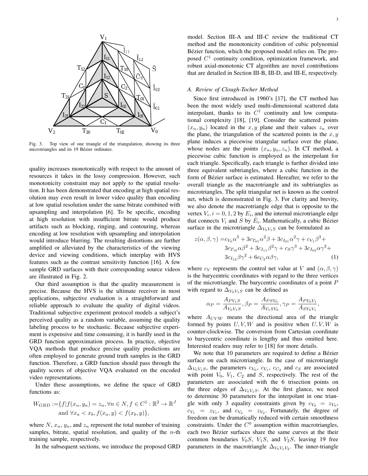
1 Modeling Generalized Rate-Distortion Functions Zhengfang Duanmu, Student Member , IEEE, W entao Liu, Student Member , IEEE, and Zhou W ang, F ellow , IEEE Abstract —Many multimedia applications requir e precise un- derstanding of the rate-distortion characteristics measured by the function relating visual quality to media attributes, for which we term it the generalized rate-distortion (GRD) function. In this study , we explore the GRD behavior of compr essed digital videos in a three-dimensional space of bitrate, resolution, and viewing device/condition. Our analysis on a large-scale video dataset rev eals that empirical parametric models are systemat- ically biased while exhaustive search methods r equire excessi ve computation time to depict the GRD surfaces. By exploiting the properties that all GRD functions share, we develop an Robust Axial-Monotonic Clough-T ocher (RAMCT) interpolation method to model the GRD function. This model allo ws us to accurately reconstruct the complete GRD function of a source video content from a moderate number of measurements. T o further reduce the computational cost, we pr esent a novel sampling scheme based on a probabilistic model and an information measure. The proposed sampling method constructs a sequence of quality queries by minimizing the overall informati veness in the remaining samples. Experimental results show that the proposed algorithm signifi- cantly outperforms state-of-the-art appr oaches in accuracy and efficiency . Finally , we demonstrate the usage of the proposed model in three applications: rate-distortion curve prediction, per - title encoding profile generation, and video encoder comparison. Index T erms —Quality-of-experience (QoE) of end users; con- tent distribution; Clough-T oucher interpolation; quadratic pro- gramming; statistical sampling . I . I N T RO D U C T I O N R A TE-DIST OR TION theory provides the theoretical foun- dations for lossy data compression and are widely employed in image and video compression schemes. Many multimedia applications require precise measurements of rate- distortion functions to characterize source signal and maximize user Quality-of-Experience (QoE). Examples of applications that explicitly use rate-distortion measurements are codec ev aluation [1], rate-distortion optimization [2], video quality assessment (VQA) [3], encoding representation recommenda- tion [4]–[7], and QoE optimization of streaming videos [8], [9]. Digital videos usually undergo a variety of transforms and processes in the content deli very chain, as sho wn in Fig. 1. T o address the growing heterogeneity of display de- vices, contents, and access network capacity , source videos are encoded into different bitrates, spatial resolutions, frame rates, and bit depths before transmitted to the client. In an adaptiv e streaming video distribution en vironment [10], based on the bandwidth, buf fering, and computation constraints, client devices adapti vely select a proper video representation The authors are with the Department of Electrical and Computer Engi- neering, Uni versity of W aterloo, W aterloo, ON N2L 3G1, Canada (e-mail: { zduanmu, w238liu, zhou.wang } @uwaterloo.ca). on a per-time segment basis to download and render . Each process influences the visual quality of a video in a dif ferent way , which can be jointly characterized by a generalized rate- distortion (GRD) function. In general, this attribute-distortion mapping comprises several complex factors, such as source content, operation mode/type of encoder , rendering system, and human visual system (HVS) characteristics. In this w ork, we assume the GRD surface is a function f : R 2 → R J , where the input of the function is the video representation consisting of bitrate and spatial resolution, the output of the function is the perceptual video quality at different viewing condition, and J represents the number of viewing devices, respectiv ely . Furthermore, the GRD function is content- and encoder-dependent. Despite the tremendous gro wth in computational multimedia ov er the last fe w decades, estimating a GRD function is difficult, expensi ve, and time-consuming. Specifically , probing the quality of a single sample in the GRD space inv olves sophisticated video encoding and quality assessment, both of which are expensiv e processes. For example, the recently announced highly competiti ve A V1 video encoder [11] and video quality assessment model VMAF [12] could be over 1000 times and 10 times slower than real-time for full high- definition (1920 × 1080) video content. Given the massive volume of multimedia data on the Internet, the real challenge is to produce an accurate estimate of the GRD function with a minimal number of samples. W e aim to develop a GRD function estimation framew ork with three desirable properties: • Accuracy: It produces asymptotically unbiased estimation of GRD function, independent of the source video com- plexity and the encoder mechanism. • Speed: It requires a minimal number of samples to reconstruct a full GRD function. • Mathematical soundness: The GRD model has to be mathematically well-behav ed, making it readily applica- ble to a variety of computational multimedia applications. T o achiev e accuracy , we analyze the properties that all GRD functions share, based on which we formulate the GRD function approximation problem as a quadratic programming problem. The solution of the optimization problem provides an optimal interpolation model lying in the theoretical GRD function space. T o achiev e speed , we propose an efficient sampling algorithm that constructs a set of queries to max- imize the expected information gain. The sampling scheme results in a unique sampling sequence in variant to source content, enabling parallel encoding and quality assessment processes. T o achiev e mathematical soundness , the GRD model is inherited from the Clough-T oucher (CT) interpolation 2 S ou r c e V ide o S e r ve r P r e - pr oc e s s ing ( R e s a mple ) L os s y C omp r e s s ion C li e nt D e c om pr e s s ion P os t - pr oc e s s ing ( R e s a mple ) E nc od e d R e pr e s e nta ti on R e nd e r e d V ide o R e c e i ve d E nc od e d R e pr e s e nta ti on V i de o D is tr ibution N e tw or k Fig. 1. Flo w diagram of video deli v ery chain. (a) (b) (c) Fig. 2. Samples of generalized rate-distortion surf aces for dif ferent video content. method, and the function is dif ferentiable e v erywhere on the domain of interests. Extensi v e e xperiments demonstrate that the resulting GRD function estimation frame w ork achie v es consistent impro v ement in speed and accurac y compared to the e xisting methods. The superiority and usefulness of the proposed algorithm are also e vident by three applications. I I . R E L A T E D W O R K Although rate-distortion theory has been successfully em- plo yed in man y multimedia applications, the research in the GRD surf ace modeling has only become a scientific field of study in the past decade. Existing methods can be roughly cate gorized based on their assumptions about the s hape of a GRD function. The first model class only mak es weak assumptions about the properties of the GRD functions. F or e xample, [6] assumes the continuity of GRD functions and apply linear interpolation to estimate the response function af- ter densely sampling the video representation space. Ho we v er , the e xhausti v e search process is com putationally e xpensi v e, not to mention the number of samples required increases e xponentially with respect to the dimension of input space. By contrast, the second class of models mak e strong a priori assumptions about the form of the GRD function to alle viate the need of e xcessi v e training samples. F or e xample, [3] assumes the video quality e xhibits an e xponential relationship with respect to the quantization step, spatial resolution, and frame rate. Alternati v ely , T oni et al. [5], [13] deri v ed a reciprocal function to model the GRD function. Similarly , [7] modeled the rate-quality curv e at each spatial resolution with a log arithmic function. A significant limitation of these models is that domains of the analytic functional forms ar e restricted only to the bitrate dimension and se v eral discrete resolutions, lacking the fle xibility to incorporate other dimensions such as frame rate and bit depth, and the capability to predict the GRD beha viors at no v el resolutions. In addition to the specific limitations the tw o kinds of models may respecti v ely ha v e, the y suf fer from the same problem that the training samples in the GRD space are either manually pick ed or randomly selected, ne glecting the dif fer - ence in the informati v eness of samples. While man y recent w orks ackno wledge the importance of GRD function [4]– [7], a careful analysis and modeling of the response has yet to be done. W e wish to address this v oid. In doing so, we seek a good compromise between 1) global and rigid models depending on random training samples and 2) local and indefinite models requiring e xhausti v e search in the video representation space. I I I . M O D E L I N G G E N E R A L I Z E D R A T E - D I S T O R T I O N F U N C T I O N S W e be gin by stating our assumptions. Our first assumption is that the GRD function is smooth. In theory , the Shannon lo wer bound, the infimum of the required bitrate to achie v e a certain quality , is guaranteed to be continuous with respect to the tar get distortion [14]. On the other hand, successi v e change in the spatial resolution w ould gradually de viate the frequenc y component and entrop y of the source signal, re sulting in smooth trans ition in the percei v ed quality . In practice, man y subjecti v e e xperiments ha v e empirically sho wn the smoothness of GRD functions [3], [15]. Furthermore, it is beneficial to impose C 1 continuity on GRD functions for better mathemat- ical properties. F or instance, the GRD surf ace is desired to be dif ferentiable in man y multimedia applications [5], [9]. Our second assumption is that the GRD functi on is axial- monotonic 1 . According to the rate-distortion theory [14], video 1 In this w ork, we use rate-distortion function and rate-quality function interchangeably . W ithout loss of generality , we assume the function f to be axial monotonically increasing. If f is axial monotonically decreasing, we replace the gi v en response with the function f max − f , where f max is the maximum v alue of quality . 3 V 2 V 0 V 1 T 12 T 21 T 10 T 01 T 02 T 20 I 21 I 22 I 01 I 02 I 12 I 11 C 2 C 0 C 1 S Fig. 3. T op vie w of one triangle of the triangulation, sho wing its three microtriangles and its 19 B ´ ezier ordinates. quality increases monotonically with respect to the amount of resources it tak es in the lossy compression. Ho we v er , such monotonicity constraint may not apply to the spatial resolu- tion. It has b e en demonstrated that encoding at high spatial res- olution may e v en result in lo wer video quality than encoding at lo w spatial resolution under the same bitrate combined with upsampling and interpolation [6]. T o be specific, encoding at high resolution with insuf ficient bitrate w ould produce artif acts such as blocking, ringing, and contouring, whereas encoding at lo w resolution with upsampling and interpolation w ould introduce blurring. The resulting distortions are further amplified or alle viated by the characteristics of the vie wing de vice and vie wing conditions, which interplay with HVS features such as the contrast sensiti vity function [16]. A fe w sample GRD surf aces with their corresponding source videos are illustrated in Fig. 2. Our third assumption is that the quality measurement is precise. Because the HVS is the ultimate recei v er in most applications, subjecti v e e v aluation is a straightforw ard and reliable approach to e v aluate the quality of digital videos. T raditional subjecti v e e xperiment protocol models a subject’ s percei v ed quality as a random v ariable, assuming the quality labeling process to be stochastic. Because subjecti v e e xperi- ment is e xpensi v e and time consuming, it is hardly used in the GRD function approximation process. In practice, objecti v e VQA methods that produce precise quality predictions are often emplo yed to generate ground truth samples in the GRD function. Therefore, a GRD function should pass through the quality scores of objecti v e VQA e v aluated on the encoded video representations. Under these assumpti ons, we define the space of GRD functions as: W GR D := { f | f ( x n , y n ) = z n , ∀ n ∈ N , f ∈ C 1 : R 2 → R J and ∀ x a < x b , f ( x a , y ) < f ( x b , y ) } , where N , x n , y n , and z n represent the total number of training samples, bitrate, spatial resolution, and quality of the n -th training sample, respecti v ely . In the subsequent sections, we introduce the proposed GRD model. Section III-A and III-C re vie w the traditional CT method and the monotonicity condition of cubic polynomial B ´ ezier function, which the proposed model relies on. The pro- posed C 1 continuity condition, optimization frame w ork, and rob ust axial-monotonic CT algorithm are no v el contrib utions that are detailed in Section III-B, III-D, and III-E, respecti v ely . A. Re vie w of Clough-T oc her Method Since first introduced in 1960’ s [17], the CT method has been the mos t widely used multi-dimensional scattered data interpolant, thanks to its C 1 continuity and lo w computa- tional comple xity [18], [19]. Consider the scattered points ( x n , y n ) located in the x, y plane and their v alues z n o v er the plane, the triangulation of the scattered points in the x, y plane induces a piece wise triangular surf ace o v er the plane, whose nodes are the points ( x n , y n , z n ) . In CT method, a piece wise c ub i c function is emplo yed as the interpolant for each triangle. Specifical ly , each triangle is further di vided into three equi v alent subtriangles, where a cubic function in the form of B ´ ezier surf ace is estimated. Hereafter , we refer to the o v erall triangle as the macrotriangle and its subtriangles as microtriangles. The split triangular net is kno wn as the control net, which is demonstrated in Fig. 3. F or clarity and bre vity , we also denote the macrotriangle edge that is opposite to the v erte x V i , i = 0 , 1 , 2 by E i , and the internal microtriangle edge that connects V i and S by ˆ E i . Mathematically , a cubic B ´ ezier surf ace in the microtriangle ∆ V 0 V 1 S can be formulated as z ( α , β , γ ) = c V 0 α 3 + 3 c T 01 α 2 β + 3 c I 01 α 2 γ + c V 1 β 3 + 3 c T 10 α β 2 + 3 c I 11 β 2 γ + c S γ 3 + 3 c I 02 α γ 2 + 3 c I 12 β γ 2 + 6 c C 2 α β γ , (1) where c V represents the control net v alue at V and ( α , β , γ ) is the barycentric coordinates with re g ard to the three v ertices of the microtriangle. The barycentric coordinates of a point P with re g ard to ∆ V 0 V 1 S can be defined as α P = A P V 1 S A V 0 V 1 S , β P = A P S V 0 A V 1 S V 0 , γ P = A P V 0 V 1 A S V 0 V 1 , where A U V W means the directional area of the triangle formed by points U , V , W and is positi v e when U , V , W is counter -clockwise. The con v ersion from Cartesian coordinate to barycentric coordinate is length y and thus omitted here. Interested readers may refer to [18] for more details. W e note that 10 parameters are required to define a B ´ ezier surf ace on each microtriangle. In the case of microtriangle ∆ V 0 V 1 S , the parameters c V 0 , c V 1 , c C 2 and c S are associated with point V 0 , V 1 , C 2 and S , respecti v ely . The rest of the parameters are associated with the 6 trisection points on the three edges of ∆ V 0 V 1 S . At the first glance, we need to determine 30 parameters for the interpolant in one trian- gle with only 3 equality constraints gi v en by c V 0 = z V 0 , c V 1 = z V 1 , and c V 2 = z V 2 . F ortunately , the de gree of freedom can be dramati cally reduced with certain smoothness constraints. Under the C 0 assumption within macrotriangles, each tw o B ´ ezier surf aces share the same curv es at the their common boundaries V 0 S , V 1 S , and V 2 S , l ea ving 19 free parameters in the macrotriangle ∆ V 0 V 1 V 2 . The inner -triangle 4 C 1 continuity remov es 7 additional degree of freedoms by enforcing the shaded neighboring microtriangles in Fig. 3 to be coplanar [20]. T o ensure inter -triangle C 1 continuity , a stan- dard approach is to assume the cross-boundary deriv ativ es of the neighboring macrotriangles to be collinear , which further reduces the degree of freedom to 9. T aking into account the three known values at V 0 , V 1 , and V 2 , we ev entually ha ve 6 unknown parameters in each macrotriangle. Although the gradients at vertices is not always a v ailable in practice, in most cases they can be estimated by considering the kno wn values not only in the vertices of the triangle in question, but also in its neighbors. The most commonly used method is to estimate the gradients by minimizing the second-order deri v ativ es along all B ´ ezier curves [21]. Readers who are interested in the details of the CT method may refer to [18], [19], [21], [22]. The original CT method suffers from at least three limi- tations in approximating GRD functions. First, it picks the normal of the edges as the direction of cross-boundary deri v a- tiv e d e E i . Howe ver , this choice gi ves an interpolant that is not in variant under affine transforms. This has some undesirable consequences: for a very narrow triangle, the spline can de- velop huge oscillations [22]. Second, the interpolant composite of piece-wise B ´ ezier polynomials is not axial-monotonic, ev en when the giv en points are axial monotonic. Third, the CT algorithm achieves the external smoothness by estimating the gradients at three vertices V i , i = 0 , 1 , 2 , and by assuming the normal deriv ativ e at the triangle boundary E i to be linear . The linear assumption is some what arbitrary and may violate monotonicity we want to achiev e. W e will address the three limitations in the subsequent sections. B. Affine-In variant C1 Continuity In this section, we propose an affine in v ariant CT in- terpolant. Instead of the normal deri vati ve at the triangle boundary E i , we consider d e E i to be parallel to ~ C i ¯ i C , i. e. c P i =( x P i − x V i ) d x V i + ( y P i − y V i ) d y V i + z V i (2a) c C i = θ kj c T j k + θ j k c T kj + η i d e E i (2b) c I i 2 = 1 3 [( x I i 1 − x V i ) + ( x T ki − x ∗ j ) + ( x T j i − x ∗ k )] d x V i + 1 3 [( y I i 1 − y V i ) + ( y T ki − y ∗ j ) + ( y T j i − y ∗ k )] d y V i + 1 3 ( x T ij − x ∗ k ) d x V j + 1 3 ( y T ij − y ∗ k ) d y V j + 1 3 η k d e E k + 1 3 ( x T ik − x ∗ j ) d x V k + 1 3 ( y T ik − y ∗ j ) d y V k + 1 3 η j d e E j + 1 3 [ z V i + ( θ ki z V i + θ ik z V k ) + ( θ ij z V j + θ j i z V i )] (2c) c S = 1 9 2 X i =0 [( x I i 1 − x V i ) + 2( x T ki − x ∗ j ) + 2( x T j i − x ∗ k )] d x V i + 1 9 2 X i =0 [( y I i 1 − y V i ) + 2( y T ki − y ∗ j ) + 2( y T j i − y ∗ k )] d y V i + 2 9 2 X i =0 η i d e E i + 1 9 2 X i =0 [(1 + 2 θ j i + 2 θ ki ) z V i ] , (2d) where P i ∈ { T ij , T ik , I i 1 } , x ∗ i = ( x ¯ C i − x C i )( x V j y V k − x V k y V j ) − ( x V k − x V j )( x C i y ¯ C i − x ¯ C i y C i ) ( x ¯ C i − x C i )( y V k − y V j ) − ( y ¯ C i − y C i )( x V k − x V j ) , y ∗ i = ( y ¯ C i − y C i )( x V j y V k − x V k y V j ) − ( y V k − y V j )( x C i y ¯ C i − x ¯ C i y C i ) ( x ¯ C i − x C i )( y V k − y V j ) − ( y ¯ C i − y C i )( x V k − x V j ) , η i = q ( x C i − x ∗ i ) 2 + ( y C i − y ∗ i ) 2 , θ kj = x T kj − x ∗ i x T kj − x T j k , θ j k = x T j k − x ∗ i x T j k − x T kj , d x V i and d y V i are partial deriv ati ves of the B ´ ezier surface at V i and { i, j, k } is a cyclic permutation of { 0 , 1 , 2 } . Since this quantity transforms similarly as the gradient under af fine transforms, the resulting interpolant is af fine-in variant [22]. W e also lift the unwanted linear constraints on the cross- boundary deri vati ves, elev ating the number of parameters in a macrotriangle back to 9. In summary , the equality constraints in (2) can be factorized into the matrix form for simplicity c = Rd + f , (3) where c ∈ R 16 × 1 , R ∈ R 16 × 9 , d ∈ R 9 × 1 , f ∈ R 16 × 1 , c and d represent the values of control net and unkno wn deriv ativ es, respectiv ely . Therefore, finding the interpolant of the macrotriangle corresponds to determining the 9 unkno wn parameters in d . Besides the inner macrotriangle constraints, we also want to keep d e E i consistent across the triangle boundary to ensure external C 1 smoothness. As a result, the following equality constraints need to be added for each edge with adjacent triangles d e E i + d e ¯ E i = 0 . (4) Combining (3) and (4), we conclude that the resulting function is C 1 continuous and affine-in v ariant. C. Axial Monotonicity This section aims to deriv e the suf ficient constraints on d for the B ´ ezier surface in the macrotriangle ∆ V 0 V 1 V 2 to be axial-monotonic. In general, the interpolant composite of piece-wise B ´ ezier polynomials is not monotonic e ven though the sampled points are monotonic. Se veral works ha ve been done to deriv e sufficient conditions for a univ ariate or biv ariate B ´ ezier function [23], [24]. W e adopt the suf ficient condition proposed in [24], where it was proved that the cubic B ´ ezier surface in a microtriangle is axial-monotonic when all the 6 triangular patches of its control net ( e .g. ∆ I 02 I 12 S , ∆ C 2 I 11 I 12 , ∆ C 2 I 01 I 02 , ∆ V 1 T 10 I 11 , ∆ T 10 T 01 C 2 , and ∆ T 01 V 0 I 01 in ∆ V 0 V 1 S ) are axial-monotonic. By combining the sufficient conditions in all three microtriangles and the inner triangle continuity , we obtain ( y V i − y V k ) c T ij + ( y V j − y V i ) c T ik ≤ ( y V j − y V k ) z V i (5a) ( y V k − y V j ) c I i 1 + ( y V i − y V k ) c C k + ( y V j − y V i ) c C j ≤ 0 (5b) ( y V 2 − y V 1 ) c I 02 + ( y V 0 − y V 2 ) c I 12 + ( y V 1 − y V 0 ) c I 22 ≤ 0 (5c) ( y S − y V j ) c T ij + ( y V i − y S ) c T j i + ( y V j − y V i ) c C k ≤ 0 . (5d) 5 W e can summarize the monotonicity constraint in matrix form Gc ≤ h , (6) where G ∈ R 10 × 16 and f ∈ R 10 × 1 . Further substitute (3) into (6), we obtain the monotonicity constraint in terms of d GRd ≤ h − Gf . (7) More details on how we construct G and h are gi ven in the Appendix. D. Optimization-based Solutions T o determine the unknown deri vati ves, we propose to min- imize the total curv ature of the interpolated surface under the smoothness assumption. Directly computing the total curvature is computationally intractable. Alternativ ely , we minimize the curvature of B ´ ezier curves at the edges of each microtriangle as its approximation. Specifically , in ∆ V 0 V 1 V 2 , the objecti ve function is written as L V 0 V 1 V 2 = 1 2 P 2 i =0 R E i h ∂ 2 z ∂ E 2 i i 2 ds E i + P 2 i =0 R ˆ E i h ∂ 2 z ∂ ˆ E 2 i i 2 ds ˆ E i , (8) where the weight 1 2 is introduced to cancel the double counting of the external edges. Consider an external boundary E i , whose B ´ ezier control net coef ficients are z V j , c T j k , c T kj , and z V k . The integral of the second order deri vati ve of the B ´ ezier curv e on E i can be represented in terms of the four coefficients as Z E i  ∂ 2 z ∂ E 2 i  2 ds E i = 1 k E i k 3 Z 1 0 h z 00 E i ( t ) i 2 dt = 18 k E i k 3 (2 c 2 T j k + 2 c 2 T k j − 2 c T j k c T k j )+ − 36 k E i k 3 ( z V j c T j k + z V k c T k j ) + 12 k E i k 3 ( z 2 V j + z 2 V k + z V j z V k ) =  c T j k c T kj  " 36 k E i k 3 − 18 k E i k 3 − 18 k E i k 3 36 k E i k 3 #  c T j k c T kj  + h − 36 z V j k E i k 3 − 36 z V k k E i k 3 i  c T j k c T kj  + 12 k E i k 3 ( z 2 V j + z 2 V k + z V j z V k ) , (9) where k E i k = q ( x V j − x V k ) 2 + ( y V j − y V k ) 2 is the length of E i . Similarly , we get the other part of the objective func- tion from an internal boundary ˆ E i , whose coef ficients are z V i , c I i 1 , c I i 2 , and c S . Z ˆ E i " ∂ 2 z ∂ ˆ E 2 i # 2 ds ˆ E i = 1 k ˆ E i k 3 Z 1 0 h z 00 ˆ E i ( t ) i 2 dt = 6 k ˆ E i k 3 (6 c 2 I i 1 + 6 c 2 I i 2 + 2 c 2 S − 6 c I i 1 c I i 2 − 6 c I i 2 c S )+ 12 z V i k ˆ E i k 3 ( − 3 c I i 1 + c S ) + 12 k ˆ E i k 3 z 2 V i =  c I i 1 c I i 2 c S      36 k ˆ E i k 3 − 18 k ˆ E i k 3 0 − 18 k ˆ E i k 3 36 k ˆ E i k 3 − 18 k ˆ E i k 3 0 − 18 k ˆ E i k 3 12 k ˆ E i k 3       c I i 1 c I i 2 c S   + h − 36 z V i k ˆ E i k 3 0 12 z V i k ˆ E i k 3 i   c I i 1 c I i 2 c S   + 12 z 2 V i    ˆ E i    3 , (10) where k ˆ E i k = p ( x S − x V i ) 2 + ( y S − y V i ) 2 is the length of ˆ E i . Substitute (9) and (10) into (8), we obtain the loss function for ∆ V 0 V 1 V 2 in matrix form L V 0 V 1 V 2 = c T U V 0 V 1 V 2 c + w T V 0 V 1 V 2 c + const, (11) where U V 0 V 1 V 2 ∈ R 16 × 16 and w V 0 V 1 V 2 ∈ R 16 × 1 . Substituting c = Rd + f into (11), we get L V 0 V 1 V 2 =( Rd + f ) T U V 0 V 1 V 2 ( Rd + f )+ w T V 0 V 1 V 2 ( Rd + f ) + const = d T ( R T U V 0 V 1 V 2 R ) d + ( f T U V 0 V 1 V 2 + w T V 0 V 1 V 2 ) Rd + const. (12) In summary , finding the axial-monotonic interpolant corre- sponds to solving the following optimization problem minimize d d T ( R T U V 0 V 1 V 2 R ) d + ( f T U V 0 V 1 V 2 + w T V 0 V 1 V 2 ) Rd subject to GRd ≤ h − Gf , d e E i + d e ¯ E i = 0 . (13) Note that the constraints are linear with respect to d and R T U V 0 V 1 V 2 R is positi ve-semidefinite. Thus, finding d turns into a standard problem of quadratic programming, which can be efficiently solved by the existing conv ex programming packages [25]. E. Robust Axial-Monotonic Clough-T ocher Method Here we propose our Robust Axial-Monotonic Clough- T ocher (RAMCT) method. The inequality constraints in (6) are sufficient conditions for x -axial monotonicity . Howe ver , the sufficient conditions cannot be satisfied in some extreme cases, making the primary solution infeasible. T o relax these constraints, we introduce hinge loss to some of these inequali- ties, motiv ated by the success of Support V ector Machine [26]. 6 Specifically , the modified inequality constraints are formulated as ( y V i − y V k ) c T ij + ( y V j − y V i ) c T ik ≤ ( y V j − y V k ) z V i (14a) ( y V k − y V j ) c I i 1 + ( y V i − y V k ) c C k + ( y V j − y V i ) c C j + ξ i 1 ≤ 0 (14b) ( y V 2 − y V 1 ) c I 02 + ( y V 0 − y V 2 ) c I 12 + ( y V 1 − y V 0 ) c I 22 ≤ 0 (14c) ( y S − y V j ) c T ij + ( y V i − y S ) c T ji + ( y V j − y V i ) c C k + ξ C k ≤ 0 , (14d) where ξ ∈ R 6 × 1 and ξ ≤ 0 . Note that (14a),(14c) are identical to (5a),(5c) because they are necessary conditions of axial monotonicity (See Appendix for proof). Rewriting these constraints in the matrix form, we obtain  G J 1 O J 2   c ξ  ≤  h 0  , where G and h are the same as in (6),(7). J 2 is a 6 × 6 identity matrix, while J 1 ∈ R 10 × 6 is obtained by padding J 2 with 3 rows of zeros to its top and inserting a row of zeros between the 3rd and 4th rows of J 2 . By substituting (3) into the inequality above, we finally obtain the inequality constraints in terms of the unkno wns d and the auxiliary v ariables ξ as  GR J 1 O J 2   d ξ  ≤  h − Gf 0  . (15) The objecti ve function is then modified accordingly , L V 0 V 1 V 2 = c T U V 0 V 1 V 2 c + w T V 0 V 1 V 2 c − λ T ξ + const, (16) where λ = [ λ, λ, · · · , λ ] T is the weighting parameter . Substi- tuting c = Rd + f into (16), we get L V 0 V 1 V 2 = d T ( R T U V 0 V 1 V 2 R ) d + ( f T U V 0 V 1 V 2 + w T V 0 V 1 V 2 ) Rd − λ T ξ + const =  d T ξ T   R T U V 0 V 1 V 2 R O O O   d ξ  +  ( f T U V 0 V 1 V 2 + w T V 0 V 1 V 2 ) R − λ T   d ξ  + const. (17) Replacing (12),(6) with (17),(15) in (13), we find that the original interpolation problem remains to be a quadratic pro- gramming problem. I V . I N F O R M AT I O N - T HE O R E T I C S A M P L I N G In this section, we first explore the informativ eness of samples in the GRD space via a probabilistic model. W e then present an information-theoretic sampling strategy that optimally selects the samples, offering enormous savings in time and computational resources. Let x = ( x 1 , ..., x N ) be a vector of discrete samples on a GRD function uniformly distributed in the bitrate-resolution space, where N is the total number of sample points on the grid. Giv en that the GRD function is smooth, when the sampling grid is dense, these discrete samples provide a good description of the continuous GRD function. In particular , when the GRD function is band-limited, it can be fully Algorithm 1: Uncertainty Sampling Initialize S = ∅ ; ¯ Σ (1) = Σ ; for k := 1 to K do i ( k ) = minimize i tr( ¯ Σ ( k ) ii − ¯ σ ( k ) i T ¯ σ ( k ) i ¯ σ ( k ) ii ) ; x ( k ) = VQA(Encode( r ( k ) i )); Set S = S ∪ x ( k ) ; ¯ Σ ( k +1) = ¯ Σ ( k ) ii − ¯ σ ( k ) i T ¯ σ ( k ) i ¯ σ ( k ) ii ; if tr( ¯ Σ ( k ) ii − ¯ σ ( k ) i T ¯ σ ( k ) i ¯ σ ii ) ≤ T then Break ; end end recov ered from these samples when the sampling density is larger than the Nyquist rate. Assuming x is created from GRD functions of real-world video content, we model x as an N - dimensional random v ariable, for which the probability density function p x ( x ) ∼ N ( µ , Σ ) follows a multiv ariate Normal distribution. The total uncertainty of x is characterized by its joint entrop y given by H x ( x ) = 1 2 log | Σ | + const, (18) where | · | is the determinant operator . If the full vector x is further divided into two parts such that x =  x 1 x 2  and Σ =  Σ 11 Σ 12 Σ 21 Σ 22  , and the x 2 portion has been resolved by x 2 = a , then the remaining uncertainty is given by the conditional entropy H x 1 | x 2 ( x 1 | x 2 = a ) = 1 2 log | ¯ Σ | ) + const, (19) where ¯ Σ = Σ 11 − Σ 12 Σ − 1 22 Σ 21 . (20) As a special case, we aim to find one sample that most efficiently reduces the uncertainty of GRD estimation. This is found by minimizing the log determinant of the conditional cov ariance matrix [27] minimize i log | ¯ Σ | = minimize i log | ¯ Σ ii − ¯ σ T i ¯ σ i ¯ σ ii | , (21) where ¯ Σ =  ¯ Σ ii ¯ σ i ¯ σ T i ¯ σ ii  and i is the row index of ¯ Σ . Minimizing (21) directly is computationally e xpensiv e, es- pecially when the dimensionality is high. Alternatively , we minimize the upper bound of the conditional entrop y minimize i tr( ¯ Σ ii − ¯ σ T i ¯ σ i ¯ σ ii ) , (22) where log | ¯ Σ ii − ¯ σ T i ¯ σ i ¯ σ ii | ≤ tr( ¯ Σ ii − ¯ σ T i ¯ σ i ¯ σ ii − I ) and I denotes identity matrix. The sample with the minimum average loss in (22) over all viewing devices is most informati ve. Once the optimal sample index is obtained, we encode the video 7 0 9 0 1 8 0 2 7 0 3 6 0 4 5 0 5 4 0 0 9 0 1 8 0 2 7 0 3 6 0 4 5 0 5 4 0 1 0 − 2 1 0 − 1 1 0 0 1 0 1 1 0 2 Fig. 4. Empirical cov ariance matrix of the GRD functions. Bitrate and spatial resolution are presented in ascending order, and spatial resolution elev ates ev ery 90 samples. at the i -th representation, e valuate its quality with objective VQA algorithms, and update the conditional covariance matrix in (20). The process is applied iterativ ely until the overall uncertainty in the system is reduced below a certain threshold T . W e summarize the proposed uncertainty sampling method in Algorithm 1, where r i represents the bitrate and spatial resolution at the i -th representation. Remark : T o get a sense of what type of samples will be chosen by the proposed algorithm, we analyze sev eral influencing f actors in the objective function (22): • By the basic properties of trace, the objectiv e function in the uncertainty sampling can be f actorized as tr( ¯ Σ ii − ¯ σ T i ¯ σ i ¯ σ ii ) =tr( ¯ Σ ii ) − tr( ¯ σ T i ¯ σ i ) ¯ σ ii =tr( ¯ Σ ) − ( ¯ σ ii + 1 ¯ σ ii X j 6 = i ¯ σ 2 ij ) . Thus, tr( ¯ Σ ii − ¯ σ T i ¯ σ i ¯ σ ii ) is a decreasing function with respect to ¯ σ ii when ¯ σ ii > r P j 6 = i ¯ σ 2 ij . This indicates that samples with large uncertainty are more likely to be selected than those with small uncertainty . • According to (20), ∀ j 6 = i , ¯ σ ( k +1) j j = ¯ σ ( k ) j j − ¯ σ ( k ) 2 ij ¯ σ ( k ) ii , suggesting the rate of reduction in the uncertainty of sample j is proportional to its squared correlation with the selected sample i in the k -th iteration. Fig. 4 shows an empirical cov ariance matrix ¯ Σ estimated from our video dataset that will be detailed in the next section, from which we observe that the GRD functions typically exhibit high correlation in a local region. Combining the first observation above, we conclude that the next optimal choice of sample should be selected from the region where labeled samples are sparse. • Note that knowing that x 2 = a alters the variance, though the new variance does not depend on the specific value of a . The independence has two important consequences. First, the proposed sampling scheme is general enough to accommodate GRD estimators from all classes. More importantly , the algorithm results in a unique sampling sequence for all GRD functions. In other words, we can generate a lookup table of optimal querying order , making the sampling process fully parallelizable. V . E X P E R I M E N T S In this section, we first describe the experimental setups including our GRD function database, the implementation details of the proposed algorithm, and the e valuation criteria. W e then compare the proposed algorithm with existing GRD estimation methods. A. Experimental setups GRD Function Database: W e construct a ne w video database which contains 250 pristine videos that span a great div ersity of video content. An important consideration in selecting the videos is that they need to be representative of the videos we see in the daily life. Therefore, we resort to the Internet and elaborately select 200 ke ywords to search for creativ e common licensed videos. W e initially obtain more than 700 4K videos. Many of these videos contain significant distortions, including heavy compression artifacts, noise, blur , and other distortions due to improper operations during video acquisition and sharing. T o make sure that the videos are of pristine quality , we carefully inspect each of the videos multiple times by zooming in and remov e those videos with visible distortions. W e further reduce artifacts and other unwanted contaminations by do wnsampling the videos to a size of 1920 × 1080 pixels, from which we extract 10 seconds semantically coherent video clips. Eventually , we end up with 250 high quality videos. Using the aforementioned sequences as the source, each video is distorted by the follo wing processes sequentially: • Spatial downsample: W e do wnsample source videos using bi-cubic filter to six spatial resolutions (1920 × 1080, 1280 × 720, 720 × 480, 512 × 384, 384 × 288, 320 × 240) according to the list of Netflix certified de vices [6]. • H.264/HEVC/VP9 compression: W e encoded the down- sampled sequences using three commonly used video encoders with two-pass encoding [1], [6], [13]. The target bitrate ranges from 100 kbps to 9 Mbps with a step size of 100 kbps. In total, we obtain 540 (hypothetical reference circuit) × 250 (source) × 3 (encoder) = 405,000 test samples (currently the largest in the VQA community). W e ev aluate the quality of each video at a given spatial resolution, bitrate, and five commonly used display devices including cellphone, tablet, laptop, desktop, and TV using SSIMplus [28] for the follo wing reasons. First, SSIMplus is currently the only HVS moti vated 8 T ABLE I M S E P E R F OR M A N CE O F T H E C O M P ET I N G G R D F U NC T I O N M O DE L S W I T H D I FFE R E N T N U M B ER O F L A BE L E D S A M PL E S S E L EC T E D B Y R A N DO M S A MP L I N G ( R S ) A N D T H E P RO P O SE D U N C E RT A I N T Y S A MP L I N G ( U S ) . sample # Reciprocal [13] Logarithmic [7] PCHIP CT RAMCT RS US RS US RS US RS US RS US 20 N.A. N.A. 23.07 13.33 68.76 26.49 88.54 56.04 135.27 16.10 30 62.27 83.34 13.08 10.56 30.95 2.06 37.99 22.78 10.98 3.29 50 38.11 73.88 9.43 6.77 8.64 0.07 11.75 12.16 4.70 0.06 75 30.27 48.85 5.15 4.92 3.08 0 4.84 3.26 1.01 0 100 27.44 38.46 4.60 4.18 1.77 0 2.75 1.26 0.13 0 540 24.51 24.51 2.76 2.76 0 0 0 0 0 0 T ABLE II l ∞ P E RF O R M AN C E O F T H E C O M P ET I N G G R D F U N C TI O N M O D E LS W IT H DI FF E R EN T NU M B E R O F L A B EL E D S A M PL E S S E L E CT E D B Y R A N D OM S AM P L I NG ( R S) A ND T H E P R OP O S ED U N CE RTA IN T Y S A M PL I N G ( U S ). sample # Reciprocal [13] Logarithmic [7] PCHIP CT RAMCT RS US RS US RS US RS US RS US 20 N.A. N.A. 19.40 16.56 38.87 28.11 36.50 29.51 45.15 21.88 30 48.32 45.36 17.85 12.28 33.04 11.07 29.84 18.70 27.07 6.13 50 52.48 45.48 15.75 12.37 24.33 2.10 21.82 14.30 23.99 2.13 75 54.49 49.08 14.59 13.53 18.22 0.47 17.89 7.76 16.51 0.11 100 55.54 51.26 14.22 14.44 16.00 0.26 15.59 5.84 14.23 0 540 58.04 58.04 18.33 18.14 0 0 0 0 0 0 spatial resolution and display device-adapted VQA model that is shown to outperform other state-of-the-art quality measures in terms of accuracy and speed [28], [29]. Second, a simplified VQA model SSIM [30] has been demonstrated to perform well in estimating the GRD functions [7]. The resulting dense samples of SSIMplus are regarded as the ground truth of GRD functions (The range of SSIMplus is from 0 to 100 with 100 indicating perfect quality). Our GRD modeling approach does not constrain itself on any specific VQA methods. When other ways of generating dense ground-truth samples are a vailable, the same GRD modeling approach may also be applied. Implementation Details: W e initialize the scattered net- work with delaunay triangulation [31], inherited from CT method [17]. The balance weight λ in (16) is set to 10 − 4 . In our current experiments, the performance of the proposed RAMCT is fairly insensiti ve to variations of the value. W e employed OSQP [25] to solve the quadratic programming problem, where the maximum number of iterations is set to 10 6 . The stopping criteria threshold T is set to 540 (the total number of representation samples in the discretized GRD func- tion space) × 10 (the standard de viation of mean opinion score in the LIVE V ideo Quality Assessment database), resulting in an av erage sample number of 38. When tr (Σ) is below the threshold, we conclude that the uncertainty in the system can be explained by the disagreement between subjects. Therefore, further improvement in prediction accuracy may not be as meaningful. Since a triangulation only cov ers the conv ex hull of the scattered point set, extrapolation beyond the con ve x hull is not possible. In order to make a fair comparison, we initialize the training set S as the representations with maximum and minimum bitrates at all spatial resolutions. T o construct the co variance matrix described in Section IV as well as test the proposed algorithm, we randomly segregated the database into a training set of 200 GRD functions and a testing set with 50 GRD functions. The random split is repeated 50 times and the median performance is reported. Evaluation Criteria: W e test the performance of the GRD estimators in terms of both accuracy and rate of con vergence. Specifically , we used two metrics to ev aluate the accuracy . The mean squared error (MSE) and l ∞ norm of the error values are computed between the estimated function and the actual function for each source content. The median results are then computed ov er all testing functions. All interpolation models can fit increasingly complex GRD functions at the cost of using many parameters. What distinguishes these models from each other is the rate and manner with which the quality of the approximation varies with the number of training samples. B. P erformance W e test fiv e GRD function models including reciprocal regression [5], logarithmic regression [7], 1D piece wise cubic Hermite interpolating polynomial (PCHIP), CT interpolation, and the proposed RAMCT on the aforementioned database. T o ev aluate the performance of the uncertainty sampling algorithm, we apply it on the fiv e GRD models above and compare its performance with random sampling scheme as the baseline. For random sampling, the initial set of training sample S is set as the representations with the maximum and minimum bitrates at all spatial resolutions to allow fair comparison. The training process with random sampling was repeated 50 times and the median performance is reported. T able I and II show the prediction accuracy on the database, from which the ke y observ ations are summarized as follo ws. First, the models that assume a certain analytic functional form are consistently biased, failing to accurately fit GRD functions e ven with all samples probed. On the other hand, the existing interpolation models usually take more than 100 random samples to con ver ge, although they are asymptotically unbiased. By contrast, the proposed RAMCT model con verges with only a moderate number of samples. Second, we analyze the core contrib utors of RAMCT with deliberate selection of 9 100 200 300 400 500 600 700 bitrate 65 70 75 80 85 90 SSIMplus Actual 720x480 Actual 1280x720 Actual 960x540 (a) 100 200 300 400 500 600 700 bitrate 65 70 75 80 85 90 SSIMplus Actual 720x480 Actual 1280x720 Actual 960x540 Linear prediction 960x540 (b) 100 200 300 400 500 600 700 bitrate 65 70 75 80 85 90 SSIMplus Actual 720x480 Actual 1280x720 Actual 960x540 RAMCT prediction 960x540 (c) Fig. 5. Prediction of RD curv e of no v el resolution from kno wn RD curv es of other resolutions. (a) Ground truth RD curv es; (b) Prediction of 960 × 540 RD curv e from 720 × 480 and 1280 × 720 curv es using linear interpolation; (c) Prediction of 960 × 540 RD curv e using the proposed method. competing models. Specifically , the 1D monotonic interpolant PCHIP significantly outperforms the 2D generic interpolant CT , suggesting the importance of axial monotonicity . RAMCT achie v es e v en better performance by e xploiting the 2D struc- ture and jointly modeling the GRD functions. Third, we observ e strong generalizability of the proposed uncertainty sampling strate gy e vident by the significant impro v ement o v er random sampling on all models. The performance impro v e- ment is most salient on the proposed model. In general, RAMCT is able to accurately model GRD functions with only 30 labeled samples, based on which the reciprocal model merely ha v e suf ficient kno wn v ariables to initialize fitting. T o g ain a concrete impression, we also recorded the e x ecution time of the entire GRD estimation pipeline including video encoding, objecti v e VQA, and GRD function approximation with the competing algorithms on a computer with 3.6GHz CPU and 16G RAM. RAMCT with uncertainty sampling tak es around 10 minut es to reduce l ∞ belo w 5, which is more than 100 times f aster than the tradition re gression models with random sampling. V I . A P P L I C A T I O N S The application scope of GRD model is much broader than VQA. Here we demonstrate three use cases of the proposed model. A. Rate-Distortion Curve at No vel Resolutions Gi v en a set of rate-distortion curv es at multiple resolutions, it is desirable to predict the rate-distortion performance at no v el resolutions, especially when there e xists a mismatch between the support ed vie wing de vice of do wnstream content deli v ery netw ork and the recommended encoding profiles. T raditional methods linearly interpolate the rate-distortion curv e at no v el resolutions [6], ne glecting the characteristics of GRD functions. Fig. 5 compares t h e linearly interpolated and RAMCT -interpolated rate-distortion curv es at 960 × 540 with the ground truth SSIMplus curv e, from which we ha v e se v eral observ ations. First, the linearly interpol ated curv e shares the same intersection with the neighboring curv es at 740 × 480 and 1280 × 720, inducing consistent bias to the prediction. The proposed RAMCT model is able to accurately predict the T ABLE III l ∞ P E R F O R M A N C E O F T H E C O M P E T I N G G R D F U N C T I O N M O D E L S W I T H D I FF E R E N T N U M B E R O F L A B E L E D S A M P L E S S E L E C T E D B Y R A N D O M S A M P L I N G ( R S ) A N D T H E P R O P O S E D U N C E R T A I N T Y S A M P L I N G ( U S ) . Resolution l ∞ MSE Linear RAMCT Linear RAMCT 640 × 360 7.68 3.12 7.89 1.56 960 × 540 7.66 4.83 6.61 3.14 1600 × 900 8.77 7.87 5.18 4.98 A v erage 8.04 5.27 6.56 3.23 quality at the intersection of the neighboring curv es by taking all kno wn rate-distortion curv es into consideration. Second, the linearly interpolated rate-distortion curv e al w ays lies between its neighboring curv es, suggesting that the predicted quality at an y bitrate is lo wer than the quality on one of its neighboring curv es. This beha vior contradicts the f act that each resolution may ha v e a bitrate re gion in which it outperforms other resolu- tions [6]. On the contrary , RAMCT better preserv es the general trend of resolution-quality curv e at dif ferent bitrate, thanks to the re gularization imposed by the C 1 condition at gi v en nodes. Third, RAMCT outperforms the linear interpolation model in predicting the ground truth rate-distortion curv e across all bitrates. The e xperimental results also justify the ef fecti v eness of the C 1 and smoothness prior used in RAMCT . T o further v alidate the performance of the proposed GRD model at no v el spatial resolutions, we predict the rate- distortion curv es of 20 randomly selected source videos from the dataset at three no v el resolutions (640 × 360, 960 × 540, and 1600 × 900). The e v aluated bitrate ranges from 100 kbps to 9 Mbps with a step size of 100 kbps. The results are listed in T able III. W e can observ e that RAMCT outperforms the linear model [6] with a clear mar gin at no v el resolutions. B. P er -T itle Encoding Pr ofile Gener ation T o o v ercome the heterogeneity in users’ netw ork conditions and display de vices, video ser vice pro viders often encode videos at m ultiple bitrates and spatial resolutions. Ho we v er , the selection of the encoding profiles are either hard-coded, resulting in sub-optimal QoE due to the ne gligence of the dif ference in source video comple xities, or selected based on interacti v e objecti v e measurement and subjecti v e judgement 10 0 2000 4000 6000 bitrate 70 75 80 85 90 95 SSIMplus Netflix Apple Microsoft Proposed (a) T itle with lo w comple xity 0 2000 4000 6000 bitrate 70 80 90 SSIMplus Netflix Apple Microsoft Proposed (b) T itle with moderate comple xity 0 2000 4000 6000 bitrate 40 50 60 70 80 90 SSIMplus Netflix Apple Microsoft Proposed (c) T itle with high comple xity Fig. 6. Bitrate ladders generated by the recommendations and the proposed algorithm for three contents. T ABLE IV A V E R A G E B I T R A T E S A V I N G O F E N C O D I N G P R O FI L E S . N E G A T I V E V A L U E S I N D I C A T E A C T U A L B I T R A T E R E D U C T I O N Microsoft Apple Netflix Proposed Microsoft 0 - - - Apple -25.3% 0 - - Netflix -29.3% -5.6% 0 - Proposed -62.0% -48.9% -46.8% 0 that are inconsistent and time-consuming. T o deli v er the best quality video to consumers, each title should recei v e a unique bitrate ladder , tailored to its specific comple xity characteristics. W e introduce a quality-dri v en per -title optimization frame w ork to automatically select the best encoding configurations, where the proposed GRD model serv es as the k e y component. Content deli v ery netw orks often aim to deli v er videos at certain quality le v els to satisfy dif ferent vie wers. It is ben- eficial to minimize the bitrate usage in the encoding profile when achie ving the objecti v e. Mathematically , the quality- dri v en bitrate ladder selection problem can be formulated as a constrained optimization problem. Specifically , for the i -th representation, minimize { x,y } x subject to f ( x, y ) ≥ C i , i = 1 , . . . , m, where x , y , f ( · , · ) , C i and m represent the bitrate, the s patial resolution, the GRD function, the tar get quality le v el of video representation i , and the total number of video representations, respecti v ely . Solving the optimization problem requires precise kno wledge of the GRD function. Thanks to the ef fecti v eness and dif ferentiability of RAMCT , the proposed model can be incorporated with gradient-based optimization tools [32] to solv e the per -title optimization problem. (Interested readers may refer to the appendix for more details on ho w we solv e the optimization problem). T o v alidate the proposed per -title encoding profile selection algorithm, we apply the algorithm to generate bitrate ladders using H.264 [33] for 50 randomly selected videos in the afore- mentioned dataset. W e set the tar get quality le v els { C i } 10 i =1 as { 30 , 40 , 50 , 60 , 70 , 75 , 80 , 85 , 90 , 95 } to co v er di v erse quality range and to match the total number of representations in standard recommendations [5]. F or simplicity , we optimize the representation sets for only one vie wing de vice (cellphone), while the procedure can be readily e xtended to multiple de vices to generate a more comprehensi v e representation set. In Fig. 6, we compare the rate-quality curv e of representation sets generated by the proposed algorithm, recommendations by Netflix [34], Apple [35], and Microsoft [36] for three videos with dif ferent comple xities, from which the k e y ob- serv ations are as fol lo ws. First, contrasting the hand-crafted bitrate ladders, the encoding profile generated by the proposed algorithm is content adapti v e. Specifically , the encoding bitrate increases with respect to the comple xity of the source video as ill u s trated from Fi g. 6(a) to Fig. 6(c). Second, the proposed method achie v es the highest quality at all bitrate le v els. The performance impro v ement is mainly introduced by the encod- ing strate gy at the con v e x hull encompassing the indi vidual per -resolution rate-distortion curv es [6]. T able IV pro vides a full summary of the Bjønte g aard-Delta bitrate (BD-Rate) [37], indicating the required o v erhead in bitrate to achie v e the same SSIMplus v alues. W e observ e that the proposed frame w ork outperforms the e xisting hard-coded representation sets by at least 47%. C. Codec Comparison In the past decade, there has been a tremendous gro wth in video compression algorithms, thanks to the f ast de v elopment of computational multimedia. W ith man y video encoders at hand, it becomes pi v otal to compare their performance, so as to find the best algorithm as well as directions for further adv ancement. Bjønte g aard-Delta model [37], [38] has become the most commonly used objecti v e coding ef ficienc y measure- ment. Bjønte g aard-Delta PSNR (BD-PSNR) and BD-Rate are typically computed as the dif ference in bitrate and quality (measured in PSNR) based on the interpolated rate-distortion curv es Q B D = R x H x L [ z B ( x ) − z A ( x )] dx R x H x L dx , (23a) R B D ≈ 10 R z H z L [ x B ( z ) − x A ( z )] dz R z H z L dz − 1 , (23b) where x A and x B are the log arithmic-scale bitrate, z A and z B are the quality of the interpolated reference and test bitrate 11 0 2000 50 8000 6000 100 1000 4000 2000 H264 HEVC Fig. 7. Generalized rate-distortion surfaces of H.264 and HEVC encoders for a sample source video. curves, respectiv ely . [ x L , x H ] and [ z L , z H ] are the ef fectiv e domain and range of the rate-distortion curves. Howe ver , BD- PSNR and BD-Rate do not take spatial resolution and viewing condition into consideration. Fig. 7 sho ws two GRD surf aces generated by H.264 [33] and HEVC encoders for a source video. Although H.264 performs on par with HEVC at low resolutions, it requires higher bitrate to achieve the same target quality at high resolutions. Therefore, applying BD-Rate on a single resolution is not suf ficient to fairly compare the ov erall performance between encoders. T o this regard, we propose generalized quality gain ( Q g ain ) and rate gain ( R g ain ) models as Q g ain = R U R y H y L R x H x L p ( u )[ z B ( x, y , u ) − z A ( x, y , u )] dxdy du R y H y L R x H x L dxdy , (24a) R g ain ≈ 10 R U R y H y L R z H z L p ( u )[ x B ( z,y ,u ) − x A ( z,y ,u )] dzdydu R U R y H y L R z H z L p ( u ) dzdy du − 1 , (24b) where p ( u ) , U , and [ y L , y H ] represent the probability density of vie wing de vices, the set of all de vice of interests, and the do- main of video spatial resolution, respectiv ely . The generalized Q g ain and R g ain models represent the expected quality gain and the expected bitrate gain (saving when R g ain negati ve) across all spatial resolutions and vie wing devices, leading to a more comprehensi ve e valuation of codecs. It should be noted that z A ( x, y , u ) is essentially the GRD function of codec A , which can be efficiently approximated by the proposed model. x A ( z , y , u ) can also be estimated numerically from the interpolated surface. (Interested readers may refer to the ap- pendix for more details on ho w we compute Q g ain and R g ain .) Therefore, RAMCT is a natural fit to the generalized Q g ain and R g ain models. The effect of any individual influencing factor can be obtained by taking the marginal expectation in the corresponding dimension, which is more robust than BD- PSNR and BD-Rate at a single resolution. Using the proposed measures on the aforementioned dataset, we ev aluate the performance of three video encoders, namely H.264, VP9, and HEVC. In order to simplify the e xpression, we set p ( u ) to be uniform distrib ution for fiv e display devices including cellphone, tablet, laptop, desktop, and TV in the paper . T able V shows the performance of VP9 and HEVC in terms of the proposed measures with H.264 as the reference T ABLE V P E RF O R M AN C E O F V P 9 , A N D H E V C I N TE R M S O F T H E G E N ER A L I ZE D Q gain A N D R gain M O DE L S W I T H H . 26 4 A S T H E B A SE L I NE C O DE C Codec Q gain R gain VP9 1.9 -27.5% HEVC 0.2 -15.9% codec, from which we can observe that VP9 outperforms HEVC by an a verage of 1.7 and 11% in Q g ain and R g ain , respectiv ely . The results of our objectiv e codec ev aluation are in general consistent with the recent video quality assessment results [39], [40]. V I I . C O N C L U S I O N S GRD functions represent the critical link between multi- media resource and perceptual QoE. In this work, we pro- posed a learning framework to model the GRD function by exploiting the properties all GRD functions share and the information redundancy of training samples. The framew ork leads to an efficient algorithm that demonstrates state-of-the- art performance, which we believe arises from the RAMCT model for imposing axial monotonicity , the joint modeling of the multi-dimensional GRD function for exploiting its functional structure, and the information-theoretic sampling algorithm for improving the quality of training samples. Ex- tensiv e e xperiments have shown that the algorithm is able to accurately model the function with a very small number of training samples. Furthermore, we demonstrate that the proposed GRD model plays a central role in a great variety of visual communication applications. The current work can be extended in many ways. As a basis for future work, we note that the interpolant can be readily extended to higher dimensions [22], making it applicable to more general applications. For example, in the fields of machine learning [27] and data visualization [41], flexible monotonic interpolation can pro vide re gularization and makes the model more interpretable. Another promising future direction is to de velop models that can predict GRD functions without sampling the GRD space. R E F E R E N C E S [1] D. Grois, D. Marpe, A. Mulayoff, B. Itzhaky , and O. Hadar , “Perfor- mance comparison of H.265/MPEG-HEVC, VP9, and H.264/MPEG- A VC encoders, ” in Picture Coding Symposium , 2013, pp. 394–397. [2] S. W ang, A. Rehman, Z. W ang, S. Ma, and W . Gao, “SSIM-motiv ated rate-distortion optimization for video coding, ” IEEE Tr ans. Circuits and Systems for V ideo T ech. , vol. 22, no. 4, pp. 516–529, Apr . 2012. [3] Y . Ou, Y . Xue, and Y . W ang, “Q-ST AR: A perceptual video quality model considering impact of spatial, temporal, and amplitude resolu- tions, ” IEEE T rans. Image Pr ocessing , vol. 23, no. 6, pp. 2473–2486, Jun. 2014. [4] W . Zhang, Y . W en, Z. Chen, and A. Khisti, “QoE-driven cache man- agement for HTTP adaptive bit rate streaming over wireless networks, ” IEEE T rans. Multimedia , vol. 15, no. 6, pp. 1431–1445, Oct. 2013. [5] L. T oni, R. Aparicio-Pardo, K. Pires, G. Simon, A. Blanc, and P . Frossard, “Optimal selection of adaptive streaming representations, ” ACM T rans. Multimedia Computing, Communications, and Applications , vol. 11, no. 2, pp. 1–43, Feb . 2015. [6] J. De Cock, Z. Li, M. Manohara, and A. Aaron, “Complexity-based consistent-quality encoding in the cloud, ” in Pr oc. IEEE Int. Conf. Image Pr oc. , 2016, pp. 1484–1488. 12 [7] C. Chen, S. Inguva, A. Rankin, and A. Kokaram, “ A subjective study for the design of multi-resolution ABR video streams with the VP9 codec, ” in Electronic Imaging , 2016, pp. 1–5. [8] Z. W ang, K. Zeng, A. Rehman, H. Y eganeh, and S. W ang, “Objective video presentation QoE predictor for smart adaptiv e video streaming, ” in Pr oc. SPIE Optical Engineering+Applications , 2015, pp. 95 990Y .1– 95 990Y .13. [9] C. Chen, Y . Lin, A. K okaram, and S. Benting, “Encoding bitrate optimization using playback statistics for HTTP-based adaptive video streaming, ” arXiv preprint , Sep. 2017. [10] D. I. Forum. (2013) For promotion of MPEG-D ASH 2013. [Online]. A vailable: http://dashif.org. [11] Alliance for Open Media. (2018) A v1 bitstream and decoding process specification. [Online]. A vailable: https://aomedia.org/ av1- bitstream- and- decoding- process- specification/. [12] Z. Li, A. Aaron, L. Katsavounidis, A. Moorthy , and M. Manohara. (2016) T ow ard a practical perceptual video quality metric. [Online]. A vailable: http://techblog.netflix.com/2016/ 06/tow ard- practical- perceptual- video.html. [13] C. Kreuzberger, B. Rainer , H. Hellwagner, L. T oni, and P . Frossard, “ A comparativ e study of DASH representation sets using real user characteristics, ” in Pr oc. Int. W orkshop on Network and OS Support for Digital Audio and V ideo , 2016, pp. 1–4. [14] T . Berger , “Rate distortion theory and data compression, ” in Advances in Source Coding . Springer , 1975, pp. 1–39. [15] G. Zhai, J. Cai, W . Lin, X. Y ang, W . Zhang, and M. Etoh, “Cross- dimensional perceptual quality assessment for low bit-rate videos, ” IEEE T rans. Multimedia , vol. 10, no. 7, pp. 1316–1324, Nov . 2008. [16] J. Robson, “Spatial and temporal contrast-sensiti vity functions of the visual system, ” Journal of Optical Society of America , vol. 56, no. 8, pp. 1141–1142, Aug. 1966. [17] R. Clough and T . J., “Finite element stiffness matrices for analysis of plates in bending, ” in Proceedings of Conf . on Matrix Methods in Structural Analysis , 1965. [18] P . Alfeld, “ A tri variate Clough-Tocher scheme for tetrahedral data, ” Computer Aided Geometric Design , vol. 1, no. 2, pp. 169–181, Jun. 1984. [19] I. Amidror, “Scattered data interpolation methods for electronic imaging systems: A survey , ” Journal of Electr onic Imaging , vol. 11, no. 2, pp. 157–177, Apr . 2002. [20] G. Farin, “B ´ ezier polynomials over triangles and the construction of piecewise C R polynomials, ” Brunel University Mathematics T echnical P apers collection , 1980. [21] G. M. Nielson, “ A method for interpolating scattered data based upon a minimum norm network, ” Mathematics of Computation , vol. 40, no. 161, pp. 253–271, 1983. [22] G. Farin, “ A modified Clough-Tocher interpolant, ” Computer Aided Geometric Design , vol. 2, no. 1-3, pp. 19–27, 1985. [23] N. Fritsch and R. Carlson, “Monotone piece wise cubic interpolation, ” SIAM Journal on Numerical Analysis , vol. 17, no. 2, pp. 238–246, 1980. [24] L. Han and L. Schumaker , “Fitting monotone surfaces to scattered data using c1 piecewise cubics, ” SIAM Journal on Numerical Analysis , vol. 34, no. 2, pp. 569–585, Apr . 1997. [25] B. Stellato, G. Banjac, P . Goulart, A. Bemporad, and S. Boyd, “OSQP: An operator splitting solver for quadratic programs, ” ArXiv pr eprint arXiv:1711.08013 , Nov . 2017. [26] C. Cortes and V . V apnik, “Support-vector networks, ” Mac hine learning , vol. 20, no. 3, pp. 273–297, Sep. 1995. [27] C. Bishop, P attern Recognition and Machine Learning . Berlin, Heidelberg: Springer-V erlag, 2006. [28] A. Rehman, K. Zeng, and Z. W ang, “Display de vice-adapted video Quality-of-Experience assessment, ” in Pr oc. SPIE , 2015, pp. 939 406.1– 939 406.11. [29] Z. Duanmu, K. Ma, and Z. W ang, “Quality-of-Experience of adaptive video streaming: Exploring the space of adaptations, ” in Pr oc. ACM Int. Conf. Multimedia , 2017, pp. 1752–1760. [30] Z. W ang, A. Bovik, H. Sheikh, and E. Simoncelli, “Image quality assessment: From error visibility to structural similarity , ” IEEE T rans. Image Pr ocessing , vol. 13, no. 4, pp. 600–612, Apr . 2004. [31] B. Delaunay , “Sur la sphere vide, ” Izv . Akad. Nauk SSSR, Otdelenie Matematicheskii i Estestvennyka Nauk , vol. 7, no. 793-800, pp. 1–2, Oct. 1934. [32] M. Grant and S. Boyd. (2014) CVX: Matlab software for disciplined con vex programming, version 2.1. [Online]. A vailable: http://cvxr .com/ cvx. [33] T . Wie gand, G. J. Sullivan, G. Bjontegaard, and A. Luthra, “Overview of the h. 264/avc video coding standard, ” IEEE Tr ans. Circuits and Systems for V ideo T ech. , vol. 13, no. 7, pp. 560–576, Jul. 2003. [34] A. Aaron, Z. Li, M. Manohara, D. J. Cock, and D. Ronca. (2015) Per-T itle encode optimization. [Online]. A vailable: https://medium.com/ netflix- techblog/per- title- encode- optimization- 7e99442b62a2. [35] Apple. (2016) Best practices for creating and deploying HTTP liv e streaming media for iPhone and iPad. [Online]. A vailable: http://is.gd/LBOdpz. [36] G. Michael, T . Christian, H. Hermann, C. W ael, N. Daniel, and B. Stefano, “Combined bitrate suggestions for multi-rate streaming of industry solutions, ” 2013. [Online]. A vailable: http: //alicante.itec.aau.at/am1.html. [37] G. Bjøntegaard, “Calculation of average PSNR differences between rd- curves, ” Austin, TX, USA, T ech. Rep. VCEG-M33, ITU-T SG 16/Q6, 13th VCEG Meeting, Apr. 2001. [38] ——, “Improvements of the BD-PSNR model, ” Berlin, Germany , T ech. Rep. VCEG-AI11, ITU-T SG 16/Q6, 35th VCEG Meeting, Jul. 2008. [39] D. V atolin, D. Kulikov , E. Mikhail, D. Stanislav , and Z. Sergey . (2017) MSU codec comparison 2017 part V: High quality encoders. [Online]. A vailable: http://www .compression.ru/video/codec comparison/hevc 2017/MSU HEVC comparison 2017 P5 HQ encoders.pdf. [40] F . Christian. (2018) Multi-codec D ASH dataset: An ev aluatation of A V1, A VC, HEVC and VP9. [Online]. A vailable: https://bitmovin.com/ av1- multi- codec- dash- dataset/. [41] M. Sarfraz and M. Hussain, “Data visualization using rational spline interpolation, ” Journal of Computational and Applied Mathematics , vol. 189, no. 1, pp. 513–525, May 2006. 1 A P P E N D I X A C O N V E R S I O N F R O M U N K N OW N S TO B ´ E Z I E R C O O R D I N A T E Summarizing (2) as matrix form, we obtain c = Rd + f More specifically , c =                          c T 01 c T 02 c I 01 c T 12 c T 10 c I 11 c T 20 c T 21 c I 21 c C 0 c C 1 c C 2 c I 02 c I 12 c I 22 c S                          R =            x V 1 − x V 0 3 y V 1 − y V 0 3 0 0 0 0 0 0 0 x V 2 − x V 0 3 y V 2 − y V 0 3 0 0 0 0 0 0 0 x V 1 + x V 2 − 2 x V 0 9 y V 1 + y V 2 − 2 y V 0 9 0 0 0 0 0 0 0 0 0 x V 2 − x V 1 3 y V 2 − y V 1 3 0 0 0 0 0 0 0 x V 0 − x V 1 3 y V 0 − y V 1 3 0 0 0 0 0 0 0 x V 0 + x V 2 − 2 x V 1 9 y V 0 + y V 2 − 2 y V 1 9 0 0 0 0 0 0 0 0 0 x V 0 − x V 2 3 y V 0 − y V 2 3 0 0 0 0 0 0 0 x V 1 − x V 2 3 y V 1 − y V 2 3 0 0 0 0 0 0 0 x V 0 + x V 1 − 2 x V 2 9 y V 0 + y V 1 − 2 y V 2 9 0 0 0 0 0 θ 21 ( x V 2 − x V 1 ) 3 θ 21 ( y V 2 − y V 1 ) 3 θ 12 ( x V 1 − x V 2 ) 3 θ 12 ( y V 1 − y V 2 ) 3 η 0 0 0 θ 20 ( x V 2 − x V 0 ) 3 θ 20 ( y V 2 − y V 0 ) 3 0 0 θ 02 ( x V 0 − x V 2 ) 3 θ 02 ( y V 0 − y V 2 ) 3 0 η 1 0 θ 01 ( x V 1 − x V 0 ) 3 θ 01 ( y V 1 − y V 0 ) 3 θ 10 ( x V 0 − x V 1 ) 3 θ 10 ( y V 0 − y V 1 ) 3 0 0 0 0 η 2 (3 θ 01 +1) x V 1 +(3 θ 20 +1) x V 2 − (3 θ 20 +3 θ 01 +2) x V 0 27 (3 θ 01 +1) y V 1 +(3 θ 20 +1) y V 2 − (3 θ 20 +3 θ 01 +2) y V 0 27 θ 10 ( x V 0 − x V 1 ) 9 θ 10 ( y V 0 − y V 1 ) 9 θ 02 ( x V 0 − x V 2 ) 9 θ 02 ( y V 0 − y V 2 ) 9 0 η 1 3 η 2 3 θ 01 ( x V 1 − x V 0 ) 9 θ 01 ( y V 1 − y V 0 ) 9 (3 θ 10 +1) x V 0 +(3 θ 21 +1) x V 2 − (3 θ 10 +3 θ 21 +2) x V 1 27 (3 θ 10 +1) y V 0 +(3 θ 21 +1) y V 2 − (3 θ 10 +3 θ 21 +2) y V 1 27 θ 12 ( x V 1 − x V 2 ) 9 θ 12 ( y V 1 − y V 2 ) 9 η 0 3 0 η 2 3 θ 20 ( x V 2 − x V 0 ) 9 θ 20 ( y V 2 − y V 0 ) 9 θ 21 ( x V 2 − x V 1 ) 9 θ 21 ( y V 2 − y V 1 ) 9 (3 θ 02 +1) x V 0 +(3 θ 12 +1) x V 1 − (3 θ 02 +3 θ 12 +2) x V 2 27 (3 θ 02 +1) y V 0 +(3 θ 12 +1) y V 1 − (3 θ 02 +3 θ 12 +2) y V 2 27 η 0 3 η 1 3 0 (6 θ 02 +1) x V 0 +(6 θ 12 +1) x V 1 − (6 θ 02 +6 θ 12 +2) x V 2 27 (6 θ 02 +1) y V 0 +(6 θ 12 +1) y V 1 − (6 θ 02 +6 θ 12 +2) y V 2 27 (6 θ 10 +1) x V 0 +(6 θ 21 +1) x V 2 − (6 θ 10 +6 θ 21 +2) x V 1 27 (6 θ 10 +1) y V 0 +(6 θ 21 +1) y V 2 − (6 θ 10 +6 θ 21 +2) y V 1 27 (6 θ 02 +1) x V 0 +(6 θ 12 +1) x V 1 − (6 θ 02 +6 θ 12 +2) x V 2 27 (6 θ 02 +1) y V 0 +(6 θ 12 +1) y V 1 − (6 θ 02 +6 θ 12 +2) y V 2 27 2 η 0 3 2 η 1 3 2 η 2 3            d =             d x V 0 d y V 0 d x V 1 d y V 1 d x V 2 d y V 2 d e E 0 d e E 1 d e E 2             f =                           z V 0 z V 0 z V 0 z V 1 z V 1 z V 1 z V 2 z V 2 z V 2 θ 21 z V 1 + θ 12 z V 2 θ 02 z V 2 + θ 20 z V 0 θ 10 z V 0 + θ 01 z V 1 ( θ 20 + θ 10 +1) z V 0 + θ 21 z V 1 + θ 02 z V 2 3 θ 10 z V 0 +( θ 21 + θ 01 +1) z V 1 + θ 12 z V 2 3 θ 20 z V 0 + θ 01 z V 1 +( θ 12 + θ 02 +1) z V 2 3 (2 θ 20 +2 θ 10 +1) z V 0 +(2 θ 21 +2 θ 01 +1) z V 1 +(2 θ 12 +2 θ 02 +1) z V 2 3                           2 A P P E N D I X B D E TA I L S O F E Q UA L I T Y C O N S T R A I N T Summarizing (5) as matrix form, we obtain Gc ≤ h , where G =         y V 0 − y V 2 y V 1 − y V 0 0 0 0 0 0 0 0 0 0 0 0 0 0 0 0 0 0 y V 1 − y V 0 y V 2 − y V 1 0 0 0 0 0 0 0 0 0 0 0 0 0 0 0 0 0 y V 2 − y V 1 y V 0 − y V 2 0 0 0 0 0 0 0 0 0 0 y V 2 − y V 1 0 0 0 0 0 0 0 y V 1 − y V 0 y V 0 − y V 2 0 0 0 0 0 0 0 0 0 y V 0 − y V 2 0 0 0 y V 1 − y V 0 0 y V 2 − y V 1 0 0 0 0 0 0 0 0 0 0 0 0 y V 1 − y V 0 y V 0 − y V 2 y V 2 − y V 1 0 0 0 0 0 0 0 0 0 0 0 0 0 0 0 0 0 y V 2 − y V 1 y V 0 − y V 2 y V 1 − y V 0 0 y S − y V 1 0 0 0 y V 0 − y S 0 0 0 0 0 0 y V 1 − y V 0 0 0 0 0 0 0 0 y S − y V 2 0 0 0 y V 1 − y S 0 y V 2 − y V 1 0 0 0 0 0 0 0 y V 2 − y S 0 0 0 0 y S − y V 0 0 0 0 y V 0 − y V 2 0 0 0 0 0         , and h =                 ( y V 1 − y V 2 ) z V 0 ( y V 2 − y V 0 ) z V 1 ( y V 0 − y V 1 ) z V 2 0 0 0 0 0 0 0                 . A P P E N D I X C D E TA I L S O F L O S S F U N C T I O N Expanding (14), we obtain U =                       18 || E 2 || 3 0 0 0 − 9 || E 2 || 3 0 0 0 0 0 0 0 0 0 0 0 0 18 || E 1 || 3 0 0 0 0 − 9 || E 1 || 3 0 0 0 0 0 0 0 0 0 0 0 36 || ˆ E 0 || 3 0 0 0 0 0 0 0 0 0 − 18 || ˆ E 0 || 3 0 0 0 0 0 0 18 || E 0 || 3 0 0 0 − 9 || E 0 || 3 0 0 0 0 0 0 0 0 − 9 || E 2 || 3 0 0 0 0 0 0 0 0 0 0 0 0 0 0 0 0 0 0 0 0 36 || ˆ E 1 || 3 0 0 0 0 0 0 0 − 18 || ˆ E 1 || 3 0 0 0 − 9 || E 1 || 3 0 0 0 0 18 || E 1 || 3 0 0 0 0 0 0 0 0 0 0 0 0 − 9 || E 0 || 3 0 0 0 18 || E 0 || 3 0 0 0 0 0 0 0 0 0 0 0 0 0 0 0 0 36 || ˆ E 2 || 3 0 0 0 0 0 − 18 || ˆ E 2 || 3 0 0 0 0 0 0 0 0 0 0 0 0 0 0 0 0 0 0 0 0 0 0 0 0 0 0 0 0 0 0 0 0 0 0 0 0 0 0 0 0 0 0 0 0 0 0 0 0 0 0 0 − 18 || ˆ E 0 || 3 0 0 0 0 0 0 0 0 0 36 || ˆ E 0 || 3 0 0 − 18 || ˆ E 0 || 3 0 0 0 0 0 − 18 || ˆ E 1 || 3 0 0 0 0 0 0 0 36 || ˆ E 1 || 3 0 − 18 || ˆ E 1 || 3 0 0 0 0 0 0 0 0 − 18 || ˆ E 2 || 3 0 0 0 0 0 36 || ˆ E 2 || 3 − 18 || ˆ E 2 || 3 0 0 0 0 0 0 0 0 0 0 0 0 − 18 || ˆ E 0 || 3 − 18 || ˆ E 1 || 3 − 18 || ˆ E 2 || 3 12 || ˆ E 0 || 3 + 12 || ˆ E 1 || 3 + 12 || ˆ E 2 || 3                       , and w V 0 V 1 V 2 =                        − 18 z V 0 || E 2 || 3 − 18 z V 0 || E 1 || 3 − 36 z V 0 || ˆ E 0 || 3 − 18 z V 1 || E 0 || 3 − 18 z V 1 || E 2 || 3 − 36 z V 1 || ˆ E 1 || 3 − 18 z V 2 || E 1 || 3 − 18 z V 2 || E 0 || 3 − 36 z V 2 || ˆ E 2 || 3 0 0 0 0 0 0 12 z V 0 || ˆ E 0 || 3 + 12 z V 1 || ˆ E 1 || 3 + 12 z V 2 || ˆ E 2 || 3                        . 3 A P P E N D I X D V I S UA L I L L U S T R AT I O N b i t r a t e 0 2 0 0 0 4 0 0 0 6 0 0 0 8 0 0 0 r e so l u t i o n 5 0 0 7 5 0 1 0 0 0 1 2 5 0 1 5 0 0 1 7 5 0 2 0 0 0 2 2 5 0 S S I M p l u s 2 0 4 0 6 0 8 0 1 0 0 (a) CT 20 iterations b i t r a t e 0 2 0 0 0 4 0 0 0 6 0 0 0 8 0 0 0 r e so l u t i o n 5 0 0 7 5 0 1 0 0 0 1 2 5 0 1 5 0 0 1 7 5 0 2 0 0 0 2 2 5 0 S S I M p l u s 2 0 4 0 6 0 8 0 1 0 0 1 2 0 (b) CT 30 iterations b i t r a t e 0 2 0 0 0 4 0 0 0 6 0 0 0 8 0 0 0 r e so l u t i o n 5 0 0 7 5 0 1 0 0 0 1 2 5 0 1 5 0 0 1 7 5 0 2 0 0 0 2 2 5 0 S S I M p l u s 2 0 4 0 6 0 8 0 1 0 0 (c) CT 40 iterations b i t r a t e 0 2 0 0 0 4 0 0 0 6 0 0 0 8 0 0 0 r e so l u t i o n 5 0 0 7 5 0 1 0 0 0 1 2 5 0 1 5 0 0 1 7 5 0 2 0 0 0 2 2 5 0 S S I M p l u s 2 0 4 0 6 0 8 0 1 0 0 (d) RAMCT 20 iterations b i t r a t e 0 2 0 0 0 4 0 0 0 6 0 0 0 8 0 0 0 r e so l u t i o n 5 0 0 7 5 0 1 0 0 0 1 2 5 0 1 5 0 0 1 7 5 0 2 0 0 0 2 2 5 0 S S I M p l u s 2 0 4 0 6 0 8 0 1 0 0 (e) RAMCT 30 iterations b i t r a t e 0 2 0 0 0 4 0 0 0 6 0 0 0 8 0 0 0 r e so l u t i o n 5 0 0 7 5 0 1 0 0 0 1 2 5 0 1 5 0 0 1 7 5 0 2 0 0 0 2 2 5 0 S S I M p l u s 2 0 4 0 6 0 8 0 1 0 0 (f) RAMCT 40 iterations Fig. 1. CT and RAMCT performance given 20, 30, and 40 training samples selected by the proposed uncertainty sampling method. Red and blue points represent the training and testing ground truth quality scores, respectively . A P P E N D I X E P R O O F O F N E C E S S A RY C O N D I T I O N S O F A X I A L M O N O TO N I C I T Y Since the interpolated surface is a continuous piece-wise cubic function, it being monotonic everywher e is equivalent to every cubic function in its own triangle being monotonic. Denote ( i, j, k ) a cyclic permutation of (0 , 1 , 2) . Consider a microtriangle ∆ V i V j S . The B ´ ezier surface z ( α, β , γ ) over the microtriangle can be formulated as (1), where the barycentric coor dinates ( α, β , γ ) ar e definded as in (2). The chain rule of derivatives shows that ∂ z ∂ x = ∂ z ∂ α ∂ α ∂ x + ∂ z ∂ β ∂ β ∂ x + ∂ z ∂ γ ∂ γ ∂ x . (A.1) From (1), we have ∂ z ∂ α =3 c V i α 2 + 6 c T ij αβ + 6 c I i 1 αγ + 3 c T j i β 2 + 3 c I i 2 γ 2 + 6 c C k β γ (A.2a) ∂ z ∂ β =3 c T ij α 2 + 6 c T j i αβ + 6 c C k αγ + 3 c V j β 2 + 3 c I j 2 γ 2 + 6 c I j 1 β γ (A.2b) ∂ z ∂ γ =3 c I i 1 α 2 + 6 c C k αβ + 6 c I i 2 αγ + 3 c I j 1 β 2 + 3 c S γ 2 + 6 c I j 2 β γ , (A.2c) and fr om (2), ∂ α ∂ x = y V j − y S 2 A , ∂ β ∂ x = y S − y V i 2 A , ∂ γ ∂ x = y V i − y V j 2 A (A.3) 4 where A denotes the ar ea of ∆ V i V j S . Substitute (A.2) and (A.3) into (A.1). After some r earrangements, we reach ∂ z ∂ x = 3 2 A [ c V 0 ( y V j − y S ) + c T ij ( y S − y V i ) + c I i 1 ( y V i − y V j )] α 2 + 3 2 A [ c T j i ( y V j − y S ) + c V j ( y S − y V i ) + c I j 1 ( y V i − y V j )] β 2 + 3 2 A [ c I i 2 ( y V j − y S ) + c I j 2 ( y S − y V i ) + c S ( y V i − y V j )] γ 2 + 6 2 A [ c T ij ( y V j − y S ) + c T j i ( y S − y V i ) + c C k ( y V i − y V j )] αβ + 6 2 A [ c I i 1 ( y V j − y S ) + c C k ( y S − y V i ) + c I i 2 ( y V i − y V j )] αγ + 6 2 A [ c C k ( y V j − y S ) + c I j 1 ( y S − y V i ) + c I j 2 ( y V i − y V j )] β γ . (A.4) z is x -axial monotonic if and only if (A.4) is nonnegative within ∆ V i V j S . Note that α, β , γ ar e all nonnegative inside or on the edge of ∆ V i V j S . One sufficient condition for (A.4) to be nonnegative is its all coef ficients are nonnegative [Han Lu et al.], as indicated in (5). T o show that (5a) and (5c) (i.e. (14a) and (14c)) are necessary conditions for ∂ z ∂ x to be nonnegative, we simply check the value of ∂ z ∂ x at three vertices of ∆ V i V j S , where ( α, β , γ ) equals (1 , 0 , 0) , (0 , 1 , 0) , and (0 , 0 , 1) , respectively . Substituting the three barycentric coordinates back into (A.4), we obtain thr ee inequalities as the necessary condition in ∆ V i V j S c V i ( y V j − y S ) + c T ij ( y S − y V i ) + c I i 1 ( y V i − y V j ) ≥ 0 (A.5a) c T j i ( y V j − y S ) + c V j ( y S − y V i ) + c I j 1 ( y V i − y V j ) ≥ 0 (A.5b) c I i 2 ( y V j − y S ) + c I j 2 ( y S − y V i ) + c S ( y V i − y V j ) ≥ 0 . (A.5c) The inner-triangle C 1 continuity implies that points V i , T ij , I i 1 , T ik are coplanar , i.e. c I i 1 = ( c V i + c T ij + c T i k ) / 3 . Substitute this equation and y S = ( y V i + y V j + y V k ) / 3 into (A.5a). Some rearrangements will yield c V i ( y V k − y V j ) + c T ij ( y V i − y V k ) + c T ik ( y V j − y V i ) ≤ 0 , (A.6) which is exactly (5a). Further , the summation of (A.5c) over all possible ( i, j, k ) gives (8c). Now we have proved (5a) and (5c) in Section 3.3 are necessary for the interplant to be axial monotonic in ∆ V 0 V 1 V 2 . A P P E N D I X F D E TA I L S O F P E R - T I T L E O P T I M I Z AT I O N According to [R1], the optimality condition of the constrained optimization problem in is achieved when the following conditions hold. First, if the quality at the lowest bitrate is higher than the tar get quality C i , the i -th optimal repr esentation is ( x L , y ∗ ) , where x L is the lowest bitrate and y ∗ = ar g max y f ( x L , y ) . Second, when the target quality cannot be obtained by the lowest bitrate, the optimality condition is fulfilled when the inequality constraints are active ( i.e. , the equation condition is achieved). Consequently , the optimization problem can be transformed into finding the bitrate x i at each resolution such that C i = f ( x i , y ) , ∀ y . W e apply the Dichotomous- based sear ch method [R1] to compute the optimal bitrate at 320 × 240, 384 × 288, 512 × 384, 640 × 360, 720 × 480, 960 × 540, 1280 × 720, 1600 × 900, 1920 × 1080 [R2]. The final bitrate is then obtained by taking the minimum value across all resolutions. A P P E N D I X G D E TA I L S O F G E N E R A L I Z E D B J Ø N T E G A A R D - D E L TA M O D E L S G.1 Generalized Bjøntegaard-Delta Quality W e apply the trapz function in Numpy [R3] to compute the numerical integration in (23a) at each r esolution fr om 500 kbps to 4000 kbps with 100 steps. The reason to select the bitrate range is that theoretically Bjøntegaard-Delta models should be computed based on actual bitrate instead of target bitrate. However , some encoders are not able to precisely control the encoding bitrate at very low or high bitrate ranges. W e find the actual bitrate variability of encoders do not exceed 10% of target bitrate within the this range, suggesting the error introduced by bitrate control is insignificant [R4]. The bitrate integration is computed at 320 × 240, 384 × 288, 512 × 384, 640 × 360, 720 × 480, 960 × 540, 1280 × 720, 1600 × 900, 1920 × 1080 [R2], and integrated over spatial r esolution to obtain the final score. G.2 Generalized Bjøntegaard-Delta Rate The computation procedure of generalized Bjøntegaard-Delta Rate at one r esolution is illustrated in Fig. 2. Specifi- cally , the shaded area S targ et can be computed as S targ et = AU C C DE + S E H LK − AU C F GH − S C F J I , 5 x L A x L B x H B x H A z L z H A B C D E F G H I J K L Fig. 2. Computation pr ocedur e of generalized Bjøntegaar d-Delta Rate at one spatial r esolution. The shaded ar ea r epr esents the overall bitrate saving. wher e S and AU C stand for the ar ea of r ectangle and ar ea under curve, r espectively . The integrations r equir e pr ecise knowledge r egar ding to the bitrates x L A , x L B , x H A , x H A , and the ef fective quality interval [ z L , z H ] at each r esolution. At any r esolution y , the integration interval is defined as z L = max ( z A ( x L , y ) , z B ( x L , y )) , z H = min ( z A ( x H , y ) , z B ( x H , y )) , in the original BD-Rate model. The bitrates ( x L A , x L B , x H A , x H A ) wher e the two rate-distortion functions achieve z L and z H ar e obtained with the Dichotomous-based sear ch method [R1]. W e apply the tr apz function in Numpy [R3] to compute the numerical ar ea under curves with step number of 100. In the end, we can integrate the overall bitrate saving over all spatial r esolutions and devices to obtain the GBD-rate. R E F E R E N C E S [R1] W eiwen Zhang, Y onggang W en, Zhenzhong Chen, an d Ashish Khisti, “QoE-driven cache management for HTTP adaptive bit rate str eaming over wir eless networks,” IEEE T rans. on Multimedia , vol. 15, no. 6, pp. 14311445, Oct. 2013. [R2] Scr eensiz. (2018) V iewport sizes and pixel densities for popular devices. [Online]. A vailable: http://scr eensiz.es/. [R3] Numpy developers. (2005) Numpy . [Online]. A vailable: http://www .numpy .or g/. [R4] Apple. (2016) Best practices for cr eating and deploying HTTP live str eaming media for iPhone and iPad. [Online]. A vailable: http://is.gd/LBOdpz.