Can learning from natural image denoising be used for seismic data interpolation?

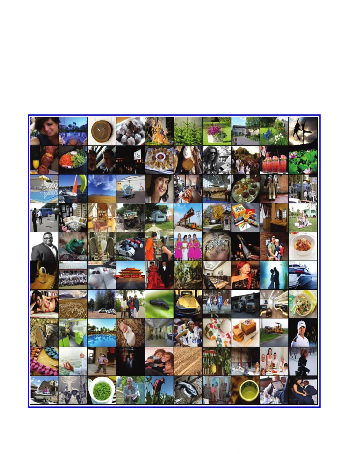
Can learning from natural image denoising be used for seismic data interpolation? Hao Zhang 1 , Xiuyan Yang 2 , and Jianwei Ma 2 ABSTRACT W e have de v eloped an interpolation method based on the denoising con volutional neural network (CNN) for seismic data. It provides a simple and ef ficient way to break through the prob- lem of the scarcity of geophysical training labe ls that are often required by deep learning methods. This new method consists of two steps: (1) training a set of CNN denoisers to learn denois- ing from natural image noisy-clean pairs and (2) inte grating the trained CNN denoisers into the project onto convex set (POCS) framework to perform seismic data interpolation. W e call it the CNN-POCS method. This method alleviates the deman ds of seismic data that requ ire shared similar feature s in the applica- tions of end-to-end deep learning for seismic data interpolation. Additionally , the adopted method is flexible a nd applicable for different types of missing traces because t he missing or down- sampling locations are not involv ed in the training step; thus, it is of a plug-and-play nature. These indicate the high gener al- izability of the proposed method and a redu ction in the necessity of problem-specific training. The prima ry results of synthe tic and field data show promising interpolation performances of the adopted CNN-POCS method in terms of the signal-to-noise ratio, dealiasing, and weak-feature reconstruction, in compari- son with the traditional f - x prediction filtering, curvelet trans- form, and block-matching 3D filtering methods. INTRODUCTION Due to existing terrain obstacles or economic restrictions, miss- ing traces in acquired seismic data, nonuniformly or uniformly , along the spatial coordinate is unavoidable, and this affect seismic in version, amplitude-versus-angle analysis, and migration. T o use these incomplete data, man y researchers have dev eloped dozens of interpolation methods to restore the missing traces. Besides frequency-space ( f - x ) prediction filtering methods ( Spitz, 1991 ; Naghizadeh and Sacchi, 2009 ), other methods based on the sparse representation of seismic data in a transform domain have been popular in the past decade because of their promising frameworks. A previous example is the project onto convex set (POCS) algo- rithm based on the Fourier transform method ( Abma and Kabir, 2006 ). In recent years, several directional wavelets, including cur- velets and shearlets, have been applied to sparsely present seismic ev ents ( Herrmann and Hennenfent, 2008 ). Y ang et al. (2012) propose seismic interpolation using the curvelet transform-based POCS algorithm. These nonadaptiv e or highly redundant trans- forms have strong anisotropic directional selectivity . Considering the characteristics of seismic data, the seislet transform was pre- sented by Fomel and Liu (2010) and later used for seismic dealias- ing interpolation based on POCS ( Gan et al., 2015 ). Dictionary learning methods ( Liang et al., 2014 ) and rank-reduction regulari- zation methods ( Trickett et al., 2010 ; Gao et al., 2013a ; Ma, 2013 ) have also been successfully applied to seismic interpolation. Yu et al. (2015) extend the data-driven tight frame (DDTF) method to 3D seismic data interpolation and later proposed the Monte Carlo DDTF method to reduce computation ( Y u et al., 2016 ). Most of these interpolation methods are suitable only for random missing cases. For re gularly subsampled seismic data with spatial aliasing, associated antialiasing techniques are included in these methods ( Naghizadeh and Sacchi, 2010 ). A machine learning method with support vector regression was successfully applied to seismic data interpolation by Jia and Ma (2017) . Deep learning (DL), which is a fast developing branch Manuscript received by the Editor 30 April 2019; revised manuscript receiv ed 22 December 2019; published ahead of production 08 January 2020; published online 7 May 2020. 1 Harbin Institute of T echnology , Center of Geophysics, Department of Mathematics and Artificial Intelligence Laboratory , Harbin 150001, China and University of California, Department of Mathematics, Los Angeles, California, USA. E-mail: hao.zhang.hit@gmail.com. 2 Harbin Institute of T echnology , Center of Geophysics, Department of Mathematics and Artificial Intelligence Laboratory , Harbin 150001, China. E-mail: yangxiuyan1995@163.com; jma@hit.edu.cn (corresponding author). © The Authors. Published by the Society of Exploration Geophysicists. All article content, except where otherwise noted (including republished material), is licensed under a Creativ e Commons Attribution 4.0 Unported License (CC BY). See http://creativecommons.or g/licenses/by/4.0/ . Distribution or reproduction of this work in whole or in part commercially or noncommercially requires full attribution of the original publication, including its digital object identifier (DOI). WA115 GEOPHYSICS, VOL. 85, NO. 4 (JUL Y -AUGUST 2020); P . W A115 – W A136, 30 FIGS., 2 T ABLES. 10.1190/GEO2019-0243.1 Downloaded 06/05/20 to 172.91.77.177. Redistribution subject to SEG license or copyright; see Terms of Use at http://library.seg.org/ Figure 1. Flowchart of the proposed CNN-POCS method. The CNN denoisers are learnt from the natural image data set rather than the seismic labeled data. Figure 2. A simple three-layered CNN denoiser network. The input is con volved with a set of filters, as shown in red above (the sliding window), to obtain a set of feature maps. Figure 3. The architecture of the CNN denoiser used in our study: s-DConv , s-dilated convolution; BN, batch normalization ( Ioffe and Szegedy , 2015 ); and ReLU, rectified linear units. Figure 4 Dila ted con v olut ion with 3 × 3n o n z e r o entr ies (the red dots) in the filte r . The 1-di late d con- vo luti on is equ iv alen t to the nor mal con voluti on op- erat ion . The RF is sho wn. WA116 Zhang et al. Downloaded 06/05/20 to 172.91.77.177. Redistribution subject to SEG license or copyright; see Terms of Use at http://library.seg.org/ of machine learning, has attracted significant attention from multi- disciplinary researchers. DL offers to learn an amount of parameters through the conv olutional neural network (CNN) to capture high- level features in the data. Recently , DL has achie ved signifi cant progress in computer vision research, including image classification ( Krizhevsky et al., 2012 ; He et al., 2016 ), denoising ( Zhang et al., 2017a ), and superresolution ( Dong et al., 2016 ; Kim et al., 2016 ). Moreover , DL has been applied to geologic feature identification ( Huang et al., 2017 ), seismic lithology detection ( Zhang et al., 2018a ), salt detection ( Guillen et al., 2015 ; W ang et al., 2018a ), an d velo city in ver sion ( W ang et al., 2018b ). For seis mic interpolation, primary attempts were m ade by W ang et al. (2019) using a residual network ( He et al., 2016 ) and by Alwon (2018) using generativ e ad- versari al networks ( Goodfellow et al., 2014 )t o r e c o v e rs e i s m i cd a t a from regularly subsampled observations. These end-to-end D L ap- proaches directly learn i nterpolation in certain mi ssing cases of s yn- thetic seismic t raining data because of a lack of training labeled dat a. The t esting of these approaches, ho we ver , requires feature similarity of the test in g data to the tr ain ing data set , wh ic h pre v en ts the prac tic al application of these DL methods in field seismic data processing. In this paper, we propose a simple and ef ficient approach for seismic data interpolation. The main idea is to integrate the deep Figure 5. One hundred images randomly selected from the natural image training set. Deep learning interpolation WA117 Downloaded 06/05/20 to 172.91.77.177. Redistribution subject to SEG license or copyright; see Terms of Use at http://library.seg.org/ denoising networks that learn denoising from natural images into the P OCS algorit hm. The moti vat ion comes fr om the intrin sic denois - ing comp onen t of the POCS algorit hm and the high perfo rma nce of deep networ ks in image denois ing. This stud y is si mila r in spirit to the stu dies using the DL netwo rk as a reg ulari zer in image proc ess ing ( Zha ng et al., 201 7b ; Liu et al., 2018 ). Ho we ver , where as the y used half -qu adra tic splitt in g ( Geman and Y ang, 1995 ) or alte rna ting dire c- tion meth od of multip lier s (ADMM) ( Boy d et al., 2011 ) to sepa rat e the regul arizatio n term from the fide lity term and then repla ce the regu larizati on term by DL netwo rks, we use DL net works to perfor m the deno isin g miss ion that exists in the POCS algor ithm. In the net- work train in g st age, instea d of le arni ng denois ing from the seismi c data , the CNNs lear n denois in g from noisy -cle an natu ral imag e pairs . In the test ing stag e, the se pretra ined CNN denois ers are inpu t into the POCS frame work to tackl e the inte rpol ation of seis mic data . This appro ach expl ore s a new tech niq ue, diffe ren t from tra nsfer learn ing ( Pan and Y ang, 2010 ), to alle viat e the lack of big dat a for DL in certa in fie lds. In the test ing stage of seismic interp olation , we obtain bett er deal iasi ng and synt heti c data reco nst ructi on for wea k ev ent s in regu lar miss ing cases than thos e using the f - x pred icti on- bas ed meth od ( Spitz, 1991 ). For fie ld data inte rpol atio n, we also compar e the CNN-PO CS meth od with two other stat e-of- the-art meth ods : the curv elet transfo rm meth od ( Can dès and Dono ho, 200 4 ; Ma and Plon ka, 2010 ) an d the bl ock- matc hi ng a nd 3D filte ring (BM3D) meth od ( Dabov et al., 2008 ) based on the POCS stra te gy . The novelty in this study can be outlined in two aspects. (1) Unlike end-to-end DL ap- proaches for seismic interpolation in which the networks must learn about subsampling, our method leverages the interpolation by iteratively attenuating noise using neural networks. Sub- sampling is not inv olved in learning, so it makes our method flexible and practical. (2) W e ob- served that using neural network denoisers that learn from natural images other than seismic data could contribute toward obtaining satisfactory seismic interpolation results. This could further help to ov ercome the huge barrier of lacking la- beled data for DL in seismic signal processing. The rest of this paper is organized as follows. In the “ Method ” section, we briefly introduce the background and the POCS framework for seismic data interpolation, and then present our CNN-POCS method, the architecture of the denoising network, as well as the denoising net- work learning strategy . In the “ Numerical experi- ments and results ” section, we show the details of the training networks and the numerical results while testing for seismic interpolation in regular and irregular sampling cases for synthetic and field data. A discussion on the CNN-POCS method is presented in the “ Discussion ” section. The conclusion is presented in the final section. 0 0.4 0.8 1.2 Time (s) 0 0.4 0.8 1.2 Time (s) 0 0.4 0.8 1.2 Time (s) 0 0.5 1 1.5 Distance (km) 0 0.5 1 1.5 Distance (km) 0 0.5 1 1.5 Distance (km) 0 0.5 1 1.5 Distance (km) 0 0.5 1 1.5 Distance (km) 0 0.5 1 1.5 Distance (km) 0 0.4 0.8 1.2 Time (s) 0 0.4 0.8 1.2 Time (s) 0 0.4 0.8 1.2 Time (s) –0.2 –0.15 –0.1 –0.05 0 0.05 0.1 0.15 0.2 –0.2 –0.15 –0.1 –0.05 0 0.05 0.1 0.15 0.2 a) b) c) d) e) f) Figure 6. Interpolation of the layered model. (a) and (d) complete data and 50% regu- larly subsampled data with a 20 m trace interval. (b) and (e) interpolated data from the f - x method ( S ∕ N ¼ 26.38 ) and the residual. (c) and (f) interpolated data from the CNN-POCS method ( S ∕ N ¼ 31.72 ) and the residual. –0.0495 0 0.0495 Wavenumber (1/m) 0 20 40 60 Frequency (Hz) –0.0495 0 0.0495 Wavenumber (1/m) 0 20 40 60 Frequency (Hz) –0.0495 0 0.0495 Wavenumber (1/m) 0 20 40 60 Frequency (Hz) –0.0495 0 0.0495 Wavenumber (1/m) 0 20 40 60 Frequency (Hz) a) b) c) d) Figure 7. The f - k spectra of the layered model. (a) Complete data, (b) regularly sampled data with a 20 m trace interval, (c) interpolated data using the f - x prediction-based method, and (d) interpolated data using the proposed CNN-POCS method. WA118 Zhang et al. Downloaded 06/05/20 to 172.91.77.177. Redistribution subject to SEG license or copyright; see Terms of Use at http://library.seg.org/ METHOD Background and the POC S framework Seismic data interpolation aimed at recovering the complete data d from an observed incomplete data d obs can be characterized as d obs ¼ P Λ d ; (1) where P Λ denotes the subsampling matrix. Seismic data can be sparsely represented by d ¼ Φ x ; (2) where Φ is a sparse transform, for example, a curvelet transform or a learned dictionary , and x is a vector of representation coefficients. Thus, we can recover the complete or dense data d by regularizing x to be sparse, that is, resolving the following optimization problem: min x k d obs − P Λ Φ x k 2 2 þ λ k x k 1 : (3) This problem is often called sparsity-promoting compressed sensing reconstruction. There are many algorithms to solve this op- timization problem, such as the well-known iterative shrinkage- thresholding (IST) algorithm ( Daubechies et al., 2004 ), its acceler- –0.0490 0 0.0490 Wavenumber (1/m) 0 20 40 60 Frequency (Hz) –0.0490 0 0.0490 Wavenumber (1/m) 0 20 40 60 Frequency (Hz) –0.0489 0 0.0489 Wavenumber (1/m) 0 20 40 60 Frequency (Hz) –0.0490 0 0.0490 Wavenumber (1/m) 0 20 40 60 Frequency (Hz) a) b) c) d) Figure 8. The f - k spectra of the layered model. (a) Regularly sampled data with a 20 m trace interval, (b) with a 40 m trace interval, (c) in- terpolated data from (b) using the f - x prediction-based method, and (d) interpolated data from (b) using the proposed CNN-POCS method. From the spectral quality point of view , the CNN-POCS method outperforms the f - x prediction-based method except for some unexpected artifacts at low frequencies. 0 0.5 1 1.5 Distance (km) 0 0.4 0.8 1.2 Time (s) –0.2 –0.1 0 0.1 0.2 0.3 0.4 0.5 0.6 Figure 9. Reconstruction residual of the CNN-POCS method. The unexpected artifacts at lo w frequencies in Figure 8d correspond to the bias at the large slope region. Table 1. S/N (dB) comparison of the four methods on field data set 1 in regular sampling cases, a significant improvement of the CNN-POCS method over other methods when a ≤ 4 . Decimating factor a ¼ 5 a ¼ 4 a ¼ 3 a ¼ 2 f - x — 5.93 — 12.15 Curvelet 3.12 4.29 6.60 10.00 BM3D 3.89 5.43 7.82 12.33 CNN-POCS 4.41 6.45 9.08 13.28 Table 2. S/N (dB) comparison of the three methods on the field data in irregular sampling cases, a significant improvement of the CNN-POCS method over other methods when a ≥ 0 . 5 . Sampling ratio a ¼ 0.1 a ¼ 0.3 a ¼ 0.5 a ¼ 0.7 Curvelet 18.26 26.54 37.16 38.03 BM3D 18.81 27.64 37.19 39.15 CNN-POCS 18.78 28.35 38.87 40.60 Deep learning interpolation WA119 Downloaded 06/05/20 to 172.91.77.177. Redistribution subject to SEG license or copyright; see Terms of Use at http://library.seg.org/ ated version, the fast iterative shrinkage-thresholding (FIST) algo- rithm ( Beck and T eboulle, 2009 ), and the split Bregman method ( Goldstein and Osher , 2009 ). The POCS algorithm is another simple iterative method to re- cover d . It can be easily derived from the IST algorithm as follows: u ð t Þ ¼ Φ T λ t ð Φ T d ð t Þ Þ ; (4) d ð t þ 1 Þ ¼ d obs þð I − P Λ Þ u ð t Þ ; (5) where the soft thresholding operator T λ is defined as T λ ð x Þ ≔ ( x − λ sign ð x Þj x j ≥ λ ; 0 j x j < λ : (6) 100 200 300 400 500 Trace number 100 200 300 400 500 Trace number 100 200 300 400 500 Trace number 100 200 300 400 500 Time sampling number 100 200 300 400 500 Time sampling number 100 200 300 400 500 Time sampling number 100 200 300 400 500 Trace number 100 200 300 400 500 Trace number 100 200 300 400 500 Time sampling number 100 200 300 400 500 Time sampling number a) b) c) d) e) Figure 11. Restored results of the four methods on field data with a regular subsampling ratio of 0.5. (a) Subsampled data; results from the (b) f - x method, S ∕ N ¼ 12.15 ; (c) curvelet method, S ∕ N ¼ 10.00 ; (d) BM3D method, S ∕ N ¼ 12.33 ; and (e) CNN-POCS method, S ∕ N ¼ 13.28 . 100 200 300 400 500 Trace number 100 200 300 400 500 Trace number 100 200 300 400 500 Time sampling number 100 200 300 400 500 Time sampling number a) b) Figure 10. T wo field data sets for the interpolation test. (a) Data set 1: North Sea marine data set for the regular sampling cases and (b) data set 2: data for the irregular sampling cases. WA120 Zhang et al. Downloaded 06/05/20 to 172.91.77.177. Redistribution subject to SEG license or copyright; see Terms of Use at http://library.seg.org/ Generally , equation 4 is regarded as a denoising procedure because the small representation coefficients, which usually corre- spond to noises in the signals, are eliminated during the iterations. Therefore, we can define the following POCS framework: u ð t Þ ¼ D σ t ð d ð t Þ Þ ; (7) d ð t þ 1 Þ ¼ d obs þð I − P Λ Þ u ð t Þ ; (8) where D σ t denotes the denoising operator with respect to the denoising parameter (noise variance) σ t . W e ignore the difference between the noise variance σ t and the thresholding parameter λ t of the sparse representation coefficients when D σ t ð d ð t Þ Þ¼ Φ T λ t ð Φ T d ð t Þ Þ , although λ t should be a function of σ t . The denoising operator is the key component of the POCS frame- work for seismic interpolation. The existing POCS algorithms for seismic interpolation, which rely on sparse representation as shown in equation 4 , are actually special cases of the POCS framework. For e xample, the POCS algorithm based on the Fourier transform ( Abma and Kabir, 2006 ), curvelet transform ( Y ang et al., 2012 ), dreamlet transform ( W ang et al., 2014 ), and seislet transform ( Gan et al., 2015 ) all perform noise attenuation by thresholding the representation coefficients in a sparse transform domain. The dictionary-based seismic interpolation methods ( Y u et al., 2015 ; Liu et al., 2017 ) also fall into this scope by thresholding the dic- tionary sparse representation coefficients. Besides the denoisers that threshold sparse representation coefficients, the POCS framework also allows general denoisers for seismic interpolation, for example, the nonlocal means ( Buades et al., 2005 ) and BM3D ( Dabov et al., 2008 ) algorithms. Another important component of the POCS frame work is the scheme on the noise level σ t . It is well-known that the POCS algo- rithm conv erges very slowly . The importance of the thresholding strategy on sparse representation coefficients was reported by Abma and Kabir (2006) when they proposed the Fourier transform POCS algorithm. Gao et al. (2010) investigate an exponentially decreasing thresholding scheme on sparse representation coefficients and ob- tain significant improvement on the convergence speed of the POCS algorithm. Intuiti vely , in our POCS framework, the noise variance σ t in each iteration should decrease because the recovered data pro- gressiv ely approximate the noise-free target. Thus, in this study , we adopt the following exponential noise level decreasing scheme for the POCS framework: σ t ¼  σ min σ max  t − 1 T − 1 · σ max ;t ¼ 1 ; 2 ; :::;T ; (9) where the two parameters σ min and σ max are manually tuned for seismic interpolation. Convolutional neural network denoiser The POCS framework allows the use of denoisers in a general sense. A denoiser with incomparable representation capacity and denoising ability is preferred because it could potentially contribute toward improving the performance of the POCS method on seismic interpolation. Bearing this in mind and the success of DL methods in image denoising, we use the CNN as the denoiser . Unlike the linear sparse transforms with thresholding used in POCS-based algorithms mentioned above, the CNNs composed of multiple 100 200 300 400 500 Trace number 100 200 300 400 500 Trace number 100 200 300 400 500 Trace number 100 200 300 400 500 Trace number 100 200 300 400 500 Time sampling number 100 200 300 400 500 Time sampling number 100 200 300 400 500 Time sampling number 100 200 300 400 500 Time sampling number a) b) c) d) Figure 12. Restored results of the three methods on the field data with an irregular sampling ratio of 0.5. (a) Subsampled data; results from the (b) cur- velet method, S ∕ N ¼ 37.16 ; (c) BM3D method, S ∕ N ¼ 37.19 ; and (d) CNN-POCS method, S ∕ N ¼ 38.87 . Deep learning interpolation WA121 Downloaded 06/05/20 to 172.91.77.177. Redistribution subject to SEG license or copyright; see Terms of Use at http://library.seg.org/ con volution operators and nonlinear activ ation functions such as the rectified linear unit (ReLU) ( Nair and Hinton, 2010 ) are more non- linearly complicated and can extract features of the data in a high- lev el context. From the mathematical vie w that we provide in Appendix A , the denoising CNNs can be regarded as a set of more advanced and adaptive data-driv en regularizers, compared with the sparse constraint regularizers. Thus, CNNs have an advantage over those linear sparse transforms in sparse representation and data denoising. The POCS framework associated with the CNN denoiser is summarized in Figure 1 . Before we detail the architecture of the denoising network used in our study , we present a basic overview of the CNN for those who are unfamiliar with it. A three-layered CNN is sho wn in Figure 2 . The input is con volved with a set of filters to obtain a set of feature maps. The activation then introduces the nonlinearity such as the sigmoid function and ReLU. The results of the activ ation 100 200 300 400 500 Trace number 100 200 300 400 500 Time sampling number 100 200 300 400 500 Time sampling number 100 200 300 400 500 Time sampling number 100 200 300 400 500 Trace number 100 200 300 400 500 Trace number 0 20 40 60 80 100 120 140 160 180 200 Time sampling number 10 80 150 Trace Number 0 20 40 60 80 100 120 140 160 180 200 Time sampling number 10 80 150 Trace Number 0 20 40 60 80 100 120 140 160 180 200 Time sampling number 10 80 150 Trace Number 40 50 60 70 80 90 100 Time sampling number 0 0.2 0.4 0.6 0.8 1 Amplitude Interpolation Original 40 50 60 70 80 90 100 Time sampling number 0 0.2 0.4 0.6 0.8 1 Amplitude Interpolation Original 40 50 60 70 80 90 100 Time sampling number 0 0.2 0.4 0.6 0.8 1 Amplitude Interpolation Original a) b) c) d) e) f) g) h) i) Figure 13. (a-c) Reconstruction errors. (d-f) Trace comparison. (g-i) Magnified view of the marked area in (d-f). The solid line represents the original trace, and the dotted line represents the reconstructed trace. Methods used from left to right are the curvelet method, BM3D method, and our proposed CNN-POCS method. WA122 Zhang et al. Downloaded 06/05/20 to 172.91.77.177. Redistribution subject to SEG license or copyright; see Terms of Use at http://library.seg.org/ Distance (km) 0 1 2 Time (s) 0 0.5 1 1.5 0 0.5 11 .5 Distance (km) 0 1 2 Time (s) 00 . 5 11 .5 Distance (km) 0 1 2 Time (s) 00 . 5 11 .5 Distance (km) 0 1 2 Time (s) a) b) c) d) Figure 14. Dense fie ld data recon structi on ex am- ple 1. (a) Observ ed data with a 12.5 m tr ace inte r- v al, (b) reco nstruc ted den se data wi th a hal ved trace inte rv al, that is, 6.25 m, usin g our CNN- POCS meth od with σ max ¼ 20 , (c) with σ max ¼ 24 ,a n d (d) with σ max ¼ 30 . The region (1 .6 – 1. 88 s and 1.0 – 1.3 75 km ) is enl arg ed at th e top- rig ht co rner . 0 0.5 1 1.5 2 Distance (km) 0 0.5 1 1.5 2 Distance (km) 0 1 2 3 Time (s) 0 1 2 3 Time (s) a) b) Figure 15. Dense field data reconstruction exam- ple 2. (a) Observed data with a 12.5 m trace inter- val and (b) zero-padded data with a 6.25 m trace interval. Deep learning interpolation WA123 Downloaded 06/05/20 to 172.91.77.177. Redistribution subject to SEG license or copyright; see Terms of Use at http://library.seg.org/ are further con volved with another set of filters, leading to higher lev el feature maps. Finally , these feature maps are conv olved to obtain the output. The convolutions lead the network to detect edges and lo wer level features in the earlier layers and more com- plex features in the deep layers in the network. In supervised DL, the networks f are forced to learn the filters/weights Θ by minimiz- ing the loss function L ð Θ Þ¼ 1 2 N X N i ¼ 1 l ð f ð y i ; Θ Þ ; x i Þ ; (10) through back-propagation using optimization algorithms, for exam- ple, the minibatch stochastic gradient descent (SGD) ( Bottou, 2010 ). In equation 10 , fð y i ; x i Þg N i ¼ 1 denote N training pairs and l denotes the discrepancy between the desired output and the net- work output. Architecture of the CNN denoiser A few iterations are necessary to ensure that the POCS frame- work conv erges. When the pretrained CNN denoisers are input into the POCS framework to perform seismic data interpolation, the deeper the network is, the more inference computation time it con- sumes. Therefore, a shallow network is preferred. W e adopt the ar- chitecture of the denoising CNN proposed by Zhang et al. (2017b) as illustrated in Figure 3 . It consists of seven layers with three differ- ent blocks, that is, one “ dilated con volution + ReLU ” block in the first layer, five “ dilated con volution + batch normalization + ReLU ” blocks in the middle layers, and one “ dilated convolution ” block in the last layer . The dilation factors of the ( 3 × 3 ) dilated convolution from the first layer to the last layer are set to 1, 2, 3, 4, 3, 2, and 1. Each middle layer has 64 feature maps. The dilated convolution ( Yu and K oltun, 2016 ) is an extension of the normal con volution, which aims to enlarge the receptive field (RF) of the networks to capture the context information while retaining the merits of normal con- volution. A dilated filter with dilation factor s can be interpreted as a sparse filter of size ð 2 s þ 1 Þ × ð 2 s þ 1 Þ . Figure 4 illustrates the di- lated convolution. Due to the residual learning strategy adopted in the network, we use the following loss function: L ð Θ Þ¼ 1 2 N X N i ¼ 1 k f ð y i ; Θ Þ − ð y i − x i Þk 2 F ; (11) where fð y i ; x i Þg N i ¼ 1 represents N noisy-clean image patch pairs. 0 0.5 1 1.5 2 Distance (km) 0 0.5 1 1.5 2 Distance (km) 0 1 2 3 Time (s) 0 1 2 3 Time (s) a) b) Figure 16. Dense field data reconstruction exam- ple 2. (a) Reconstruction using σ max ¼ 25 and (b) reconstruction using σ max ¼ 50 . Some discon- tinuity can be observed in the rectangular region in (a), and this is suppressed in (b). –0.0395 0 0.0395 Wavenumber (1/m) 0 20 40 60 Frequency (Hz) –0.0398 0 0.0398 Wavenumber (1/m) 0 20 40 60 Frequency (Hz) –0.0398 0 0.0398 Wavenumber (1/m) 0 20 40 60 Frequency (Hz) –0.0398 0 0.0398 Wavenumber (1/m) 0 20 40 60 Frequency (Hz) a) b) c) d) Figure 17. Spectrum comparison of the data in Figures 15 and 16 . (a) Original data, (b) zero-padded original data, (c) dense reconstruction using σ max ¼ 25 , and (d) dense reconstruction using σ max ¼ 50 . Differences can be observed around the boundary between (c) and (d). WA124 Zhang et al. Downloaded 06/05/20 to 172.91.77.177. Redistribution subject to SEG license or copyright; see Terms of Use at http://library.seg.org/ Learning specific denoisers with small interval noise levels The iterativ e POCS framework requires various denoiser models with dif ferent noise levels; howe ver , it is not practical to learn the CNN denoisers for all possible σ t s . Hence, we choose to train a set of 25 denoisers in the noise-level range [0, 50] with a step size of two for each model. Another reason for this choice is that in the test stage (i.e., the interpolation on seismic data), the denoiser in the POCS framework should perform its own role regardless of the noise type and noise level of its input, which is different from recov- ering the latent clean image from the noisy image with an additive Gaussian noise. Thus, inexact denoising is a reasonable strategy . NUMERICAL EXPERIMENTS AND RESUL TS In this section, we first present the data preparation and the denoising network training details. Sequentially , we use the POCS fra me wor k equi pped with the pre trai ned denois in g netwo rk to inte r- pol ate the seismi c dat a. Inter pola tions for re gula rl y an d irr egu larly sub samp led data are in clu ded in our expe rime nts. W e compare the num eric al resul ts from our meth od with se ver al state -of- the-ar t meth - ods , includ ing the curv elet and BM3D meth ods. The trad itio nal Spitz f - x pred icti on filte rin g meth od is al so used for comp arison. Training stage: Denoisers learning from natural images Training data set preparation It is widely acknowledged that CNNs generally benefit from big training data. In seismic exploration, howe ver , it is more difficult to obtain a large amount of input-label data pairs than in natural image processing. Although synthetic seismic data generated by wav e- equation modeling can be fed into CNNs as training data, the pre- trained CNNs in the testing step always require the testing data to Figure 19. One hundred training examples ex- tracted from the seismic training set. 100 150 200 250 300 350 400 450 500 550 Size 0 0.5 1 1.5 2 2.5 3 3.5 Time (s) Curvelet BM3D CNN-POCS CNN-POCS GPU Figure 18. Running time of a single denoising step using the curvelet, BM3D, and CNN denoiser on CPU and CNN denoiser on GPU. Deep learning interpolation WA125 Downloaded 06/05/20 to 172.91.77.177. Redistribution subject to SEG license or copyright; see Terms of Use at http://library.seg.org/ possess feature similarity to the training data to obtain expected re- sults ( W ang et al., 2019 ). The feature similarity requirement essen- tially hinders the practical application of CNNs in seismic data processing. Given the abundance of natural images, we assume that they contain the features that are hidden in seismic data, which can be learnt by CNNs. This assumption is verified in the “ Discussion ” section, where the denoiser learning from images is applied to seis- mic data denoising. Thus, instead of using seismic data to prepare the training data set, we generate the training data set from natural images. The natural image data set used for training CNN denoiser models includes 400 Berkeley segmentation data set (BSD) images of size 180 × 180 ( Chen and Pock, 2017 ), 400 selected images from the validation set of the ImageNet database ( Krizhevsky et al., 2012 ), and 4744 images from the W aterloo Exploration Data- base ( Ma et al., 2017 ). Figure 5 shows 100 samples drawn from this training data set. W e crop the images into small patches of size 35 × 35 , and the total number of patches for training is N ¼ 256 × 4000 . T o generate the corresponding noisy data sets, we add additive Gaussian noise to the clean patches during training. Training denoisers T o optimize the network parameter Θ , the Adam optimizer ( Kingma and Ba, 2015 ) is used with the momentum parameter β ¼ 0.9 for a minibatch size of 128. Rotation or/and flip-based data augmentation is adopted during minibatch learning. The learning rate is set to 0.001 at the start of training and then fixed at 0.0001 when the training loss stops decreasing. The training is terminated if the training loss is fixed in five sequential epochs. T o reduce the overall training time, we initialize the adjacent deno- 01 01 Shot (km) Receiver (km) 0 1 0 0.4 Time (s) Receiver (km) –12 –10 –8 –6 –4 –2 0 2 4 6 01 01 Shot (km) Receiver (km) 0 1 0 0.4 Time (s) Receiver (km) –15 –10 –5 0 5 10 01 01 Shot (km) Receiver (km) 0 1 0 0.4 Time (s) Receiver (km) –10 –8 –6 –4 –2 0 2 4 6 01 01 Shot (km) Receiver (km) 0 1 0 0.4 Time (s) Receiver (km) –10 –8 –6 –4 –2 0 2 4 6 a) b) c) d) Figure 20. Three-dimensional synthetic seismic data denoising (size 178 × 178 × 128 ). (a) Original data, (b) noisy data ( S ∕ N ¼ − 4.21 ), (c) restored result by the seismic denoiser ( S ∕ N ¼ 6.92 ), and (d) restored result by the image denoiser ( S ∕ N ¼ 10.16 ). WA126 Zhang et al. Downloaded 06/05/20 to 172.91.77.177. Redistribution subject to SEG license or copyright; see Terms of Use at http://library.seg.org/ iser with the model obtained at the previous noise lev el. It takes about three days to finish the training of the set of denoiser models in the MA TLAB (R2018a) environment with MatConvNet package ( V edaldi and Lenc, 2015 ) and an Nvidia Titan V GPU. Testing stage: Seismic data interpol ation Once the denoisers are provided, we can interpolate the seismic data by the POCS algorithm. W e consider the interpolation results from the curvelet transform method, BM3D method, and the f - x prediction filtering method for comparison with our CNN-POCS method. W e fix the number of iterations T of the POCS algorithm at T ¼ 30 for all of the denoising methods, that is, the curvelet, BM3D, and CNN denoiser methods. The parameters for interpola- tion σ max and σ min are adapted to obtain the best results possible for each experiment. In practice, we fix σ min ¼ 2 for the CNN-POCS method because the minimum noise level that the pretrained CNN denoisers can deal with is two. This setting eases the parameter fine- tuning of the CNN-POCS method to obtain better interpolated results. The signal-to-noise ratio (S/N) value that is used to judge the quality of the restoration is defined as follows: S ∕ N ¼ 10 log 10  k d 0 k 2 F k d 0 − d  k 2 F  ; (12) where d 0 and d  denote the complete data and their reconstruction, respectiv ely . Interpolation for synthetic data set Fir st, w e de mons tr ate the effec tivene ss o f our met hod in t he in - terpolation of synthetic data. Figure 6a shows the synthetic data wit h t hre e events, wh ic h i ncl ude s 19 1 trac es wi th a 10 m t rac e interval. There are 751 time samples per trace with 2 m s as the t im e int er val. Fi gu re 6d s hows t he r egul arl y sa mpl ed d ata with a 20 m trace interval, which contains many jaggies. The int e rpo la ted re sul t usi ng th e prop os ed CNN -PO CS met ho d is shown i n Fi gur e 6c , wi th th e re covere d S /N eq ual to 31 .72 dB. The r ec onst ru cti on e rro r is shown i n Fi gure 6f ,i nw h i c ht h e rec ons truc ti on re si dua l ha s a ver y sm all magn itud e. For com pa ri- son, we present the reconstruction result from the f - x met hod ( S ∕ N ¼ 26.38 d B ) and the residual in Figure 6b and 6e ,r e s p e c - tively . T o fur th er as ses s th e per for ma n ce o f the propo sed CNN - POC S m eth od, we pr ovid e t he f - k spectra in Figure 7a – 7d ,w h i c h 012 012 Shot (km) Receiver (km) 0 1 2 0 0.4 0.8 1.2 1.6 Time (s) Receiver (km) –25 –20 –15 –10 –5 0 5 10 15 20 25 012 012 Shot (km) Receiver (km) 0 1 2 0 0.4 0.8 1.2 1.6 Time (s) Receiver (km) –50 –40 –30 –20 –10 0 10 20 30 40 012 012 Shot (km) Receiver (km) 0 1 2 0 0.4 0.8 1.2 1.6 Time (s) Receiver (km) –30 –20 –10 0 10 20 30 012 012 Shot (km) Receiver (km) 0 1 2 0 0.4 0.8 1.2 1.6 Time (s) Receiver (km) –30 –20 –10 0 10 20 a) b) c) d) Figure 21. Three-dimensional field seismic data denoising (size 438 × 221 × 271 ). (a) Original data, (b) noisy data ( S ∕ N ¼ 6.99 ), (c) restored result by the seismic denoiser ( S ∕ N ¼ 11.10 ), and (d) restored result by the image denoiser ( S ∕ N ¼ 11.03 ). Deep learning interpolation WA127 Downloaded 06/05/20 to 172.91.77.177. Redistribution subject to SEG license or copyright; see Terms of Use at http://library.seg.org/ represent the spectra of the true complete data, the 50% regularly sub sam pled dat a, t he inter pol ate d r esu lt us in g th e f - x predic tion- bas ed me tho d, and the pr opo sed C N N-P OC S met hod, resp ec- tively. S pa t ial ali asi ng is ob ser ved in Fi gu re 7b for the r egul ar l y sam ple d dat a , and it i s well -re moved b y the pr opo sed me thod as s h o w ni nF i g u r e 7d , whi ch valid ate s t he dea lias in g e ffect ivenes s of our pr opo s ed met hod. W e further decimate the regularly sampled data in Figure 6d wit h a f act or of t wo, res ult ing in a 25% reg ula rly sub sam ple d data with more sever e spectral aliasing, to assess the dealiasing effect of our p rop ose d m etho d. The recover ed S/N are 1 3.98 and 13.11 dB for our proposed method and the f - x prediction- bas ed int erp ol a tio n met hod, r es p ect ively . F igur e 8a – 8d show s t he corr es pon din g s pec t ra . Fi gure 8d shows the f - k spec t ru m of the int erpo la ted dat a from our prop osed CN N-P OCS met hod , whi ch out per for ms th at fro m the f - x prediction-based method excep t fo r som e unex pec ted a rti fact s at a l ow f re que ncy . T he reconstruction residual of the CNN-POCS method is presented in Figure 9 , fro m w her e we fin d t hat th e u nexp ect ed art if ac t s i n the sp ect rum c orr esp ond to t he rec ons truc ti on bi a s at the l arge slope and large amplitude region. These testing results further illustrate the validity of interpolating from regular sparse grids to regu lar and de nse grids . Interpolation for migrated field data sets T o further prove the flexibility of the p roposed CNN-POCS m e t h o d ,w eu s et h et w om i g r a t e df i e l dd a t as e t ss h o w ni n Figure 10 . The ge ologic structure has a certain amount of com- plexity for these two data sets. Many experiments are conducted on these two data sets, and the int erpolating r esults are reported, with respect to regularly and irregularly subsampled data at different ra tios. T ab les 1 and 2 present a comparison of the S/N values for al l of the sampl ing r atios i n cases of r egular sam- pling and irregular sampling, respectively . Here, it should be noted that irregular sa mplin g randomly se lect s traces i n the regu- lar grids with a maximum trace g ap equal to the inverse of the sampling ratio. For the regular sampling cases, Figure 11 shows the results of the four methods for the subsampling ratio 50%. From the S/N value point of view , CNN-POCS produces the best result. W e compare the enlarged plot of the patch marked in Figure 10a at the bottom-right portions of Figure 11b – 11e . From the visual quality point of view , the interpolated result of CNN-POCS is consistent with the truth shown in Figure 10a . For the irregular sampling cases, Figure 12 shows the results of the three methods; the CNN-POCS method again obtains the best S/N v alue. Figure 13a – 13c presents the 0.68 1.68 Receiver (km) 0.44 0.84 1.24 Time (s) 0.68 1.68 Receiver (km) 0.44 0.84 1.24 Time (s) 0.68 1.68 Receiver (km) 0.44 0.84 1.24 Time (s) 0.68 1.68 Receiver (km) 0.44 0.84 1.24 Time (s) 0.68 1.68 Receiver (km) 0.44 0.84 1.24 Time (s) 0.68 1.68 Receiver (km) 0.44 0.84 1.24 Time (s) a) b) c) d) e) f) Figure 22. Magnification of a single slice of 3D field data. (a) and (d) original and the corrupted data. (b) and (e) the restored data by the seismic denoiser and the corresponding reconstruction error . (c) and (f) the restored data by the image denoiser and the corresponding reconstruction error . WA128 Zhang et al. Downloaded 06/05/20 to 172.91.77.177. Redistribution subject to SEG license or copyright; see Terms of Use at http://library.seg.org/ reconstruction errors and the trace comparison of the interpolated results obtained from the curvelet, BM3D, and CNN-POCS meth- ods are shown in Figure 13d – 13i . Our proposed CNN-POCS method suffers from the fewest artifacts, and the amplitude of the artifacts is the smallest. Dense field data reconstruction In a seismic survey , sometimes the acquisition trace interval is not sufficient for a specific algorithm of indoor signal processing; thus, the interpolation algorithms should be adopted to construct dense data. Figure 14a shows a land shot gather with 147 traces, and the trace interval is 12.5 m between adjacent traces. Reconstructed dense data are provided in Figure 14b – 14d with a halved trace interval using the CNN-POCS method by setting different σ max s . W e observe that the dense data are more continuous and the spatial serration effects are effectively weakened. A magnified version (1.6 – 1.88 s and 1.0 – 1.375 km) is presented at the top-right corner in each figure. Another dense reconstruction example is provided in Figures 15 , 16 , and 17 . Figure 15 shows the original field data and its zero-padded version as input to the CNN-POCS algorithm. Fig- ure 16 presents the dense reconstruction using different σ max . Some gaps remain in the dense reconstruction result using σ max ¼ 25 as the rectangles in Figure 16a , and they are well-removed in Figure 16b using σ max ¼ 50 . The f - k spectrum of these data are depicted in Figure 17 . The spectra aliasings in Figure 17a and 17b are well-suppressed in Figure 17c using σ max ¼ 25 , but some resid- uals remain around the left and right boundary . These residuals are further removed by using σ max ¼ 50 as shown in Figure 17d , yield- ing a perfect spectral aliasing suppressed result. Efficiency of the prop osed method Finally , we profile the run time of one denoising step for all meth- ods running on CPUs and a single GPU for the CNN denoiser in testing/interpolation stage in Figure 18 . The experiments are con- ducted on a sequence of data with increasing sizes on a laptop with CPU Intel i7-9750H and a single GPU GTX 1650. The CNN de- noiser takes a medium length of time on a CPU that is less than the BM3D method but more than the curvelet transform; howe ver , it is much faster on a GPU in less than 0.005 s when the input size is 550 by 550. DISCUSSION Results from the previous section show that the proposed CNN- POCS method in which the CNN denoisers are pretrained on natural images is able to produce a satisfactory interpolation quality for synthetic and field data. The data used in the tests are dominated by different features, which indicates that our proposed method does not require feature similarity among the data to be processed. Additionally , the reconstructed aliasing-free data can be beneficial Figure 23. (a-f) Intermediate outputs of all convolutional layers in ascending order, that is, from the input to the output of the network. The outputs from the first 16 channels (out of 64) are shown in each subfigure. Deep learning interpolation WA129 Downloaded 06/05/20 to 172.91.77.177. Redistribution subject to SEG license or copyright; see Terms of Use at http://library.seg.org/ to subsequent seismic data processing steps. Although the results of our study are encouraging, many questions remain to be answered further . W e discuss several interesting topics arising out of our study in this section. Is making the denoiser s learn from images really valid for seismic data? The cornerstone of our study is the assumption that natural im- ages contain the features/priors of seismic data. By making the de- noisers learn from natural images, we alleviate the lack of seismic labeled data. T o make it con vincing, we present two examples to show that the denoisers that learn from natural images (image denoisers) can get comparable performance with those that learn from seismic data (seismic denoisers) on denoising seismic noisy data. W e generate 202,496 seismic samples as a training set and 84,768 seismic samples for validating from SEG open data sets. This seismic data training set is considerably large compared with that in Y u et al. (2019) . One hundred patch examples drawn from this data set are shown in Figure 19 . W e follow the procedure of training image denoisers as described above to train the seismic de- noisers. W e test our image denoiser and seismic denoiser by 3D synthetic seismic data in Figure 20a and 3D field data in Figure 21a with all 2D slices denoised parallelly (inputting 3D seismic data into CNN as a batch). The corrupted data and restored results are shown in Figure 20b – 20d and 21b – 21d . For synthetic data, the seismic denoiser seems to fail to restore the data because of the inadequate capability of generalization, with visible noise left in the restored data, whereas our image denoiser succeeds in removing most noise and achieving S/Ns that are 3 db larger than those of the seismic denoiser . For the poststacked field data, although the image deno- iser obtains an S/N value slightly smaller than that of seismic de- noiser , we find that it can better preserve signals than the seismic denoiser as the reconstruction and residual magnifications depicted in Figure 22 . W e further provide the intermed iate outputs of all layer s in the image denois ing network when denoising the seismic data in Figure 23 for con volu tional layers and in Figure 24 for ReLU layers from the input to the output of the network. In each subfigu re, the outputs from the first 16 channels (out of 64) are presente d. W e ob- serve ho w the seismic data feature is separated from the noise an d remov ed step by step, and, finally , the random noise is retained (with the residua l learning tha t we use noise as outputs). Is the CNN-POCS method convergent ? One may be strict with the con vergenc y of the proposed CNN- POCS method and its sensibility to the parameters σ max and σ min . W e give the conditions that ensure the convergence of the POCS framework and a short proof in Appendix B , showing that the con- vergence requires that the denoisers are bounded and the σ t takes 0 as a limit. However , it is not easy to prove that the CNN denoisers Figure 24. (a-f) Intermediate outputs of all ReLU layers in ascending order, that is, from the input to the output of the network. The outputs from the first 16 channels (out of 64) are shown in each subfigure. The ev ents and noise are gradually separated. Black pixels indicate zeros, and gray/white pixels indicate positive values. WA130 Zhang et al. Downloaded 06/05/20 to 172.91.77.177. Redistribution subject to SEG license or copyright; see Terms of Use at http://library.seg.org/ we use are bounded. W e do provide some experimental clues in Figure 25 , which presents the footprints (the reconstructed S/N val- ues) of the CNN-POCS method in the iterations in different inter- polating cases. In each of these cases, the reconstructed S/N value lines of a large range of σ max finally merge. These results, to some extent, indicate that the CNN denoisers are bounded denoisers and the proposed CNN-POCS method is con vergent. W e refer readers who are interested in this part to a more recent paper by Ryu et al. (2019) , which proposes the real spectral normalization to make the network strictly satisfy Lipschitz condition with Lipschitz constant smaller than one. This Lipschitz denoiser condition is indeed stronger than the bounded denoiser condition. The theoretical proof shows that the parameter σ min in our noise level exponentially decaying strategy should be positiv ely small enough to make the CNN-POCS conv ergent, but in practice we find that fixing σ min ¼ 2 always obtains the best results. The reason for this is that the CNN denoisers learn from data at a minimum discrete noise level of two. For irregularly downsampled data with large data holes, slightly in- creasing the σ min can lead to slightly better S/N results. Interpolation for randomly subsampled data T o assess the performance of the proposed method on randomly downsampled data in which some big holes occur as always being used to test traditional interpolation methods, we further provide the experiments on the synthetic data and the marine data in Figure 10b . Randomly subsampled synthetic hyperbolic data at a ratio of 50% is shown in Figure 26 , and some big data holes can be observed ob- viously . The biggest gap is of eight traces and next to a gap of four traces, with only one data trace between each other. The interpolated results using the three methods, the curvelet, BM3D, and our CNN-POCS method, are presented in Figure 27a – 27c along with the corresponding reconstruction bias in Figure 27d – 27f . From the visual point of view , the proposed CNN-POCS method succeeds 0 0.5 1 1.5 Distance (km) 0 0.4 0.8 1.2 Time (s) Figure 26. Randomly subsampled data of the original synthetic data in Figure 6a at a sampling ratio of 50% ( S ∕ N ¼ 2.99 ). Some big data holes occur in the subsampled data. 10 02 0 3 0 Iterations 10 02 0 3 0 Iterations 10 02 0 3 0 Iterations 5 10 15 20 25 30 35 S/N value max =20 max =25 max =30 max =35 max =40 max =45 max =50 0 2 4 6 8 10 12 14 S/N value max =5 max =10 max =15 max =20 max =25 max =30 max =40 24 26 28 30 32 34 36 38 40 S/N value max =10 max =15 max =20 max =25 max =30 max =35 max =40 a) b) c) Figure 25. Rec o ns tr uc ted S/N v al u es us in g the CN N- PO CS meth od with different σ max in the iterations in different cases. (a) 50% regular subsampling on synthetic seism ic data, (b) 50% regular subsampling on field data set 1, and (c) 50% irregular subs ampling on field data set 2. Deep learning interpolation WA131 Downloaded 06/05/20 to 172.91.77.177. Redistribution subject to SEG license or copyright; see Terms of Use at http://library.seg.org/ to reconstruct all of the data at big holes except the largest hole that has the steepest slope, whereas the BM3D method almost fails to re- store the data at big holes. The curvelet method suffers from the Gibbs and boundary effects. In terms of S/N, the proposed CNN-POCS method gets the largest S/N value equal to 19.42 dB, which is more than 5 dB larger than that of the curvelet ( S ∕ N ¼ 14.32 dB ) and BM3D ( S ∕ N ¼ 13.01 dB ) methods. An example of re- constructing randomly downsampled synthetic data with two dipping events crossing each other is also provided. The synthetic complete data and the 50% randomly downsampled data are shown in Figure 28a and 28d . Some data holes are observed at/near the crossover points. The restored data and residuals using the curvelet method and our CNN-POCS method are shown in Figure 28b – 28c and Figure 28e – 28f . The S/N value of the result from the CNN-POCS method is slightly (approximately 0.5 dB) larger than that from the curvelet method. But again, we observe that the CNN-POCS method loses accuracy in restoring data at large holes especially where the slope is large. The underlying reasons caus- ing this phenomenon are two fold: The first one is about the denoising neural network; the small kernel size and shallow network architecture used in our network cannot ensure that the net- work grasps adequate and useful information from data pixels around large data holes. Thus, the convolution layers (kernel size and convolu- tion type) and the network depth should be opti- mized for better application in severely missing scenarios. The second potential reason is about the training data set; the image data set we used still lacks some characteristic features of seismic data. This encourages us to combine natural im- ages and seismic data to form a richer training data set. Finally , we present a field data example in Figure 29 , where Figure 29a shows the sub- sampled data and Figure 29b – 29d sho ws the reconstruction biases of the restored results by different methods. The proposed method obtains the best S/N value equal to 32.10 dB, which is 0.6 and 1.0 dB larger than the S/N values obtained by the curvelet and BM3D methods, respectiv ely . Simultaneously denoising and interpolating seismic data The plain/original POCS framework used in our manuscript in equations 7 and 8 implicitly assumes that the observed seismic data should have a high S/N because of the insertion of the observed seismic data. Howe ver , if the observed data are noisy , this plain POCS framework will fail to suppress the noise. T o solve this problem, 0 0.5 1 1.5 Distance (km) 0 0.4 0.8 1.2 Time (s) 0 0.5 1 1.5 Distance (km) 0 0.4 0.8 1.2 Time (s) 0 0.5 1 1.5 Distance (km) 0 0.4 0.8 1.2 Time (s) 0 0.5 1 1.5 Distance (km) 0 0.4 0.8 1.2 Time (s) 0 0.5 1 1.5 Distance (km) 0 0.4 0.8 1.2 Time (s) –0.3 –0.2 –0.1 0 0.1 0.2 0.3 0.4 0.5 –0.3 –0.2 –0.1 0 0.1 0.2 0.3 0.4 0.5 0 0.5 1 1.5 Distance (km) 0 0.4 0.8 1.2 Time (s) –0.3 –0.2 –0.1 0 0.1 0.2 0.3 0.4 0.5 a) b) c) d) e) f) Figure 27. (a-c) Restored results by the curvelet method (S/N = 14.32), BM3D method (S/N = 13.01) and our proposed CNN-POCS method (S/N = 19.42), and (d-f) the cor- responding reconstruction errors. 0 0.5 1 1.5 2 2.5 Distance (km) 0 0.4 0.8 Time (s) 0 0.5 1 1.5 2 2.5 Distance (km) 0 0.4 0.8 Time (s) 0 0.5 1 1.5 2 2.5 Distance (km) 0 0.4 0.8 Time (s) 0 0.5 1 1.5 2 2.5 Distance (km) 0 0.4 0.8 Time (s) 0 0.5 1 1.5 2 2.5 Distance (km) 0 0.4 0.8 Time (s) –0.4 –0.3 –0.2 –0.1 0 0.1 0.2 0.3 0.4 0 0.5 1 1.5 2 2.5 Distance (km) 0 0.4 0.8 Time (s) –0.4 –0.3 –0.2 –0.1 0 0.1 0.2 0.3 0.4 a) b) c) d) e) f) Figure 28. Exper imen t on syn the tic data with two dip pin g e vet s cro ssin g each other . The ori gin al ran ge of da ta val ue is [0; 255 ], we sc ale the ran ge of data valu e to [ − 1, 1] for prese ntatio n. (a and d) Origin al data and the 50% rando mly down -sa mpled dat a (S/ N = 19.8 5), la rge hole s occu r near/ at cross -o ver points ; (b an d e) rec onst ruc tion by the cur ve let meth od (S/N = 39.0 2) and the recon str uc tion res idua l; (c and f) recons tru ct ion by the CNN-PO CS me tho d (S/N = 39. 57) and the rec ons tru ctio n res idu al. WA132 Zhang et al. Downloaded 06/05/20 to 172.91.77.177. Redistribution subject to SEG license or copyright; see Terms of Use at http://library.seg.org/ Gao et al. (2013b) propose the weighted strategy and then W ang et al. (2015) propose an adaptive form. Howe ver , if we revie w the plain POCS framework above, we will find that the noise is in- jected back in each iteration by the second step, although the first denoising step has attenuated the noise. Therefore, given the denois- ing ability of the denoiser , to make sure that the final output is noise- free, a simple yet efficient way is to switch the order of the two steps, yielding the following updated framework: u ð t Þ ¼ d obs þð I − P Λ Þ d ð t Þ ; (13) d ð t þ 1 Þ ¼ D σ t ð u ð t Þ Þ : (14) If the obse rve d dat a are noise free, the upda ted POC S frame work abov e is equ i v alen t to the plai n POC S frame work. If the obser ved data are nois y , say , with a noise lev el of σ ,t h e nt om a k et h e rec onst ruc tio n well -interp ol ate d and the nois e sup pres se d, the only thin g we hav e to do is to set the param eter σ min ¼ σ to make th e den oise r att enu ate the noise eff icient ly in the last iter at ion. An exa mple of the syn thet ic hyperbo lic seismi c dat a is pr ovi ded to demon str ate the ef fic iency of the upda ted POCS frame wo rk. Fig ure 30a pre sent s the comple te da ta cor rup ted with Gaus - sian noise with a noise lev el σ ¼ 10 and Figu re 30d pres en ts the nois y 50% irre gula rl y sub samp led data. The rec onst ruc tio n usin g the cur vel et method and the CNN- POCS meth od is sho wn in Figur e 30b – 30c , and the corr espo nd - ing re co nstr uct ion r esid ual is pres en ted in Figu re 30e – 30f . The missin g data are we ll- reco n- stru ct ed and the noise is well -at te nuat ed by the CNN- PO CS method , resulti ng in an S/N val ue equ al to 20.24 dB, which is much lar ger than tha t the curve let me thod obtai ns ( S ∕ N ¼ 12.17 dB ). Limitations The proposed CNN-POCS method has its lim- itations. First, it requires multiple denoiser mod- els to deal with different noise le vels. Training such a set of denoising models is arduous. Because the noise is coupled with the truth in noisy images, the network has to learn about the noise along with image features; thus, the network cannot be adaptive to noise. It will help the network to be adaptiv e to noise if we provide information about noise to the network to sav e the effort of learning noise. The FFDNet method ( Zhang et al., 2018b ) feeds the network with a noise-level map and denoises the subi- mages to obtain a fast and flexible solution for image denoising. Thus, the burden of training multiple denoising models in the CNN-POCS method can be reduced using FFDNet. Second, the proposed CNN-POCS method loses accuracy in restoring missing seismic data at large slope and large gap regions. This is spotted in examples of interpolating sev erely decimated seismic data and –80 –60 –40 –20 0 20 40 60 80 –80 –60 –40 –20 0 20 40 60 80 100 200 300 400 500 Trace number 100 200 300 400 500 Trace number 100 200 300 400 500 Trace number 100 200 300 400 500 Trace number 100 200 300 400 500 Time sampling number 100 200 300 400 500 Time sampling number 100 200 300 400 500 Time sampling number 100 200 300 400 500 Time sampling number –80 –60 –40 –20 0 20 40 60 80 d) c) b) a) Figure 29. Randomly subsampled data and reconstruction errors using different methods. (a) Subsampled marine data with big data holes ( S ∕ N ¼ 19.00 ), (b) reconstruction error of the curvelet method (restored S ∕ N ¼ 31.43 ), (c) reconstruction error of the BM3D method (restored S ∕ N ¼ 31.04 ), and (d) reconstruction error of the CNN-POCS method (restored S ∕ N ¼ 32.10 ). 0 0.5 1 1.5 Distance (km) 0 0.4 0.8 1.2 Time (s) 0 0.5 1 1.5 Distance (km) 0 0.4 0.8 1.2 Time (s) 0 0.5 1 1.5 Distance (km) 0 0.4 0.8 1.2 Time (s) 0 0.5 1 1.5 Distance (km) 0 0.4 0.8 1.2 Time (s) 0 0.5 1 1.5 Distance (km) 0 0.4 0.8 1.2 Time (s) a) b) c) d) e) f) 0 0.5 1 1.5 Distance (km) 0 0.4 0.8 1.2 Time (s) Figure 30. Simultaneously denoising and interpolating seismic data. (a) Noisy complete data ( S ∕ N ¼ 4.80 ), (b) reconstruction using the curvelet method ( S ∕ N ¼ 12.17 ), (c) reconstruction using the CNN-POCS method ( S ∕ N ¼ 20.24 ), (d) noisy irregularly subsampled data ( S ∕ N ¼ 1.76 ), (e) reconstruction residual of the curvelet method, and (f) reconstruction residual of the CNN-POCS method. Deep learning interpolation WA133 Downloaded 06/05/20 to 172.91.77.177. Redistribution subject to SEG license or copyright; see Terms of Use at http://library.seg.org/ randomly subsampled seismic data with large data holes. W e dis- cussed two ma in rea sons for this. The fir st reason for limi tation of neur al netwo rk enco urag es us to optimi ze the archit ect ur e of den ois- ing n eural netwo rk; the seco nd rea so n for th e trai nin g data set enco ur - ages us to com bin e nat ural images with se ismi c dat a to establi sh a mor e po wer ful trainin g dat a set. Third , the ex tens ion of the prop osed meth od to 5D inte rpo lati on might be dif f icu lt if we want to dire ct ly tra in the netwo rks for 5D volu mes becaus e 5D con voluti on is not av ailab le in thos e ex isti ng DL pla tfor ms. An altern ativ e way is to tra in 3D CNN den oise rs, which we can refer to as video denois ing, and apply thes e 3D CNNs to the 5D seis mi c data alon g the oth er two axe s seque ntia ll y . Or we can also apply our 2D CNN deno ise rs to th e 5D dat a alon g the other th ree ax es seque ntia lly . CONCLUSION W e introduced a CNN-POCS method for seismic interpolation and showed that the CNN denoisers pretrained on natural images could essentially contribute to improving the seismic interpolation results. The demand for a large amount of seismic data, as required by end-to-end deep-learning interpolation approaches, was reduced by the richness of the natural labeled images. The flexibility of our method allo ws it to be adaptive to any missing trace cases. More- over , the effectiv eness of the proposed method in antialiasing can be beneficial to the subsequent seismic processing steps. W e tested this method on synthetic and field data, in which we considered regular and irregular sampling at different ratios. The CNN-POCS method is competitive in comparison with the f - x method, the curvelet method, and the BM3D method in terms of S/N values and weak feature preservation. Additionally , we showed that the CNN-POCS method is stable and not sensitive to the parameters. T raining the denoising models for the CNN-POCS method is slightly time- consuming: It takes approximately three days. W e proposed a pos- sible solution, that is, using a more state-of-art denoising network FFDNet, to resolve it. The denoisers that learn from natural images completely are excellent for seismic interpolation; howe ver, they may lose some capacity to effecti vely represent some seismic fea- tures. W e suggested a promising direction for future work, that is, mixing natural images and seismic data in the training data set for CNN denoisers. In our future work, we will further explore the ex- tension of the idea of using plug-and-play CNNs that learn from images to seismic inv ersion and imaging problems. ACKNOWLEDGME NTS W e thank S. Y u for the very helpful discussions, and we thank Y . Sui, X. W ang, Z. Liu, and W . W ang for their help and suggestions. The work was supported in part by the National Key Research and Dev elopment Program of China under grant 2017YFB0202902 and the NSFC under grant 41625017 and grant 41804102. H. Zhang was additionally supported by the China Scholarship Council. DATA AND MATERIALS AVAILABILIT Y Data associated with this research are av ailable and can be obtained by contacting the corresponding author . APPENDIX A MATHEMATICAL VIEW FOR USING CNNS Mathematically , the seismic interpolation problem can be written in a general form: min d g ð d Þþk P Λ d − d obs k 2 2 ; (A-1) where g is the prior function and a well-known example is g ð d Þ¼k d k 1 . By the linear approximation technique, the iterativ e algorithm for solving this problem can be deriv ed as d ð t þ 1 Þ ¼ arg min d g ð d Þþ < P Λ d ð t Þ − d obs ; d − d ð t Þ > þ 1 2 δ t k d − d ð t Þ k 2 2 ¼ arg min d g ð d Þþ 1 2 δ t k d − ð d ð t Þ − δ t ð P Λ d ð t Þ − d obs ÞÞk 2 2 : (A-2) If we denote u ð t Þ ¼ d ð t Þ − δ t ð P Λ d ð t Þ − d obs Þ then we get the algorithm u ð t Þ ¼ d ð t Þ − δ t ð P Λ d ð t Þ − d obs Þ ; (A-3) d ð t þ 1 Þ ¼ arg min d g ð d Þþ 1 2 δ t k d − u ð t Þ k 2 2 : (A- 4) T reating u ð t Þ as the “ noisy ” image, the second equation mini- mizes the residue between u ð t Þ and the “ clean ” image d using the prior g ð d Þ . More precisely , according to Bayesian probability , the second equation corresponds to denoising the image u ð t Þ by a Gaussian denoiser with noise level ffiffiffi ffi δ t p ( Lebrun et al., 2013 ). If g ð d Þ¼k d k 1 , then sparse transform can be used in this step. For unknown prior function g ð d Þ , it encourages us to use Gaussian CNN denoisers to learn it from data. APPENDIX B CONVERGENCE CONDITION AND PROOF Before we giv e the convergence condition of the POCS frame- work and its proof, a definition of the bounded denoiser is stated below; it will help us with our main convergence result. D EFINITION 1. ( Chan et al., 2017 ). Bounded denoiser: A bounded denoiser with a parameter σ is a function D σ ∶ R n → R n such that for any input x ∈ R n , k D σ ð x Þ − x k 2 ≤ n σ 2 C; (B-1) for some univ ersal constant C independent of n and σ . The main con vergence result of the POCS framework is as follows. T HEOREM 1. The POCS framework demonstrates a fixed-point conv ergence if the denoiser is bounded and σ t → 0 as t → ∞ . That is, there exists d  such that k d ð t Þ − d  k 2 → 0 . Proof. T o get the proof, we need to show the following fact first: WA134 Zhang et al. Downloaded 06/05/20 to 172.91.77.177. Redistribution subject to SEG license or copyright; see Terms of Use at http://library.seg.org/ P Λ d ð t Þ ¼ P Λ d obs þ P Λ ð I − P Λ Þ u ð t − 1 Þ ¼ P Λ d obs ¼ d obs ; (B-2) with P Λ ð I − P Λ Þ¼ 0 because the subsampling matrix P Λ is a diagonal matrix with entries being 0 or 1. Thus, we have k d ð t þ 1 Þ − d ð t Þ k 2 2 ¼k d obs þð I − P Λ Þ D σ t ð d ð t Þ Þ − d ð t Þ k 2 2 ¼k ð I − P Λ Þð D σ t ð d ð t Þ Þ − d ð t Þ Þk 2 2 ≤ k D σ t ð d ð t Þ Þ − d ð t Þ k 2 2 ≤ n σ 2 t C: (B-3) Therefore, as t → ∞ , k d ð t þ 1 Þ − d ð t Þ k 2 → 0 . Hence, f d ð t Þ g ∞ t ¼ 1 is a Cauchy sequence. Because a Cauchy sequence in R n always con verges, there must exist d  such that k d ð t Þ − d  k 2 → 0 . □ REFERENCES Abma, R., and N. Kabir, 2006, 3D interpolation of irregular data with a POCS algorithm: Geophysics, 71 , no. 6, E91 – E97, doi: 10.1190/1 .2356088 . Alw on, S., 2018, Gen erat i ve adv ers aria l networ ks in sei smi c data proces sin g: 88t h Ann ual Interna tio nal Meet ing, SEG, Expand ed Abstra cts, 1991 – 19 95, doi : 10.11 90/ se gam2 018-299 6002.1 . Beck, A., and M. T eboulle, 2009, A fast iterativ e shrinkage-thresholding algorithm for linear inverse problems: SIAM Journal on Imaging Scien- ces, 2 , 183 – 202, doi: 10.1137/080716542 . Bottou, L., 2010, Large-scale machine learning with stochastic gradient descent: Proceedings of COMPST A T ’ 2010, Springer , 177 – 186. Boyd, S., N. Parikh, E. Chu, B. Peleato, and J. Eckstein, 2011, Distributed optimization and statistical learning via the alternating direction method of multipliers: Fou ndations and T rends in Machine Learning , 3 ,1 – 122, doi: 10.1561/2200000016 . Buades, A., B. Coll, and J.-M. Morel, 2005, A non-local algorithm for image denoising: Proceedings of IEEE Computer Society Conference on Com- puter V ision and Pattern Recognition, IEEE, 60 – 65. Candès, E. J., and D. L. Donoho, 2004, New tight frames of curvelets and optimal representations of objects with piecewise c2 singularities: Communication s o n Pure and Applied Mathematic s , 57 , 219 – 266, doi: 10.1002/cpa.v57:2 . Chan, S. H., X. W ang, and O. A. Elgendy , 2017, Plug-and-play ADMM for image restoration: Fixed-point convergenc e and applications: IEEE T ransaction s o n Comput ational Imaging , 3 ,8 4 – 98, doi: 10.1109/TCI .2016.2629286 . Chen, Y ., and T . Pock, 2017, Trainable nonlinear reaction diffusion: A flex- ible frame work for fast and effective image restoration: IEEE Transaction s on Pa ttern Analysis and Machine Intelligenc e , 39 , 1256 – 1272, doi: 10 .1109/TP AMI.2016.2596743 . Dabov , K., A. Foi, V . Katkovnik, and K. Egiazarian, 2008, Image restoration by sparse 3D transform-domain collaborative filtering: Image Processing: Proceedings SPIE, 6812 , 681207, doi: 10.1117/12.766355 . Daubechies, I., M. Defrise, and C. De Mol, 2004, An iterative thresholding algorithm for linear inv erse problems with a sparsity constraint: Commu- nications on Pure and Applied Mathem atics , 57 , 1413 – 1457, doi: 10 .1002/cpa.20042 . Dong, C., C. C. Loy , K. He, and X. T ang, 2016, Image super-resolution using deep convolutional networks: IEEE T ransaction s o n P a ttern Analy- sis and Machin e Intelligenc e , 38 , 295 – 307, doi: 10.1109/TP AMI.2015 .2439281 . Fomel, S., and Y . Liu, 2010, Seislet transform and seislet frame: Geophysics, 75 , no. 3, V25 – V38, doi: 10.1190/1.3380591 . Gan, S., S. W ang, Y . Chen, Y . Zhang, and Z. Jin, 2015, Dealiased seismic data interpolation using seislet transform with low-frequenc y constraint: IEEE Geoscience and Remote Sensing Letters , 12 , 2150 – 2154, doi: 10 .1109/LGRS.2015.2453119 . Gao, J., A. Stanton, M. Naghizadeh, M. D. Sacchi, and X. Chen, 2013b, Conv ergence improvement and noise attenuation considerations for be- yond alias projection onto con vex sets reconstruction: Geophysical Pro- specting, 61 , 138 – 151, doi: 10.1111/j.1365-2478.2012 .01103.x . Gao, J., M. D. Sacchi, and X. Chen, 2013a, A fast reduced-rank interpolation method for prestack seismic volumes that depend on four spatial dimen- sions: Geophysics, 78 , no. 1, V21 – V30, doi: 10.1190/geo2012-0038.1 . Gao, J.-J., X.-H. Chen, J.-Y . Li, G.-C. Liu, and J. Ma, 2010, Irregular seismic data recons tru cti on based on e xpo nent ial thresho ld model of POCS metho d: Ap pl i e d G eo ph ys i c s , 7 ,2 2 9 – 23 8, doi: 10. 1007 /s11 770-010 -0 246 -5 . Geman, D., and C. Y ang, 1995, Nonlinear image recovery with half-quad- ratic regularization: IEEE T ransactions on Image Processin g , 4 , 932 – 946, doi: 10.1109/83.392335 . Goldstein, T ., and S. Osher, 2009, The split Bregman method for l1-regu- larized problems: SIAM Journal on Imaging Sciences , 2 , 323 – 343, doi: 10.1137/080725891 . Goodfellow , I., J. Pouget-Abadie, M. Mirza, B. Xu, D. W arde-Farley , S. Ozair, A. Courville, and Y . Bengio, 2014, Generative adversarial nets: Advances in Neural Information Processing Systems, 2672 – 2680. Guillen, P ., G. Larrazabal, G. González, D. Boumber, and R. V ilalta, 2015, Supervised learning to detect salt body: 85th Annual International Meet- ing, SEG, Expanded Abstracts, 1826 – 1829, doi: 10.1190/segam2015- 5931401.1 . He, K., X. Zhang, S. Ren, and J. Sun, 2016, Deep residual learning for image recognition: Proceedings of the IEEE Conference on Computer V ision and Pattern Recognition, 770 – 778. Herrmann, F . J., and G. Hennenfent, 2008, Non-parametric seismic data recovery with curvelet frames: Geophysic al Journal Internation al , 173 , 233 – 248, doi: 10.1111/j.1365-246X.2 007.03698.x . Huang, L., X. Dong, and T . E. Clee, 2017, A scalable deep learning platform for identifying geologic features from seismic attributes: The Leading Edge, 36 , 249 – 256, doi: 10.1190/tle36030249.1 . Ioffe, S., and C. Szegedy , 2015, Batch normalization: Accelerating deep network training by reducing internal cov ariate shift: Proceeding of the 32nd International Conference on Machine Learning, 448 – 456. Jia, Y ., and J. Ma, 2017, What can machine learning do for seismic data processing? An interpolation application: Geophysics, 82 , no. 3, V163 – V177, doi: 10.1190/geo2016-0300.1 . Kim, J., J. Kwon Lee, and K. Mu Lee, 2016, Accurate image super-reso- lution using very deep convolutional networks: Proceedings of the IEEE Conference on Computer Vision and Pattern Recognition, 1646 – 1654. Kingma, D. P ., and J. Ba, 2015, Adam: A meth od for stocha stic optimizati on: Proceedin gs of the Internatio nal Conferen ce on Learnin g Represent ations . Krizhevsk y , A., I. Sutskever , and G. E. Hinton, 2012, Imagenet classification with deep con volutional neural networks: Advances in Neural Informa- tion Processing Systems, 1097 – 1105. Lebrun, M., A. Buades, and J.-M. Morel, 2013, A nonlocal Bayesian image denoising algorithm: SIAM Journal on Imaging Sciences , 6 , 1665 – 1688, doi: 10.1137/120874989 . Liang, J., J. Ma, and X. Zhang, 2014, Seismic data restoration via data-driv en t i g h tf r a m e :G e o p h y s i c s , 79 ,n o .3 ,V 6 5 – V74, doi: 10.1190/geo20 13-0252. 1 . Liu, J., T . Kuang, and X. Zhang, 2018, Image reconstruction by splitting deep learning regularization from iterative inversion: Presented at the International Conference on Medical Image Computing and Computer- Assisted Intervention, Springer, 224 – 231. Liu, L., G. Plonka, and J. Ma, 2017, Seismic data interpolation and denois- ing by learning a tensor tight frame: Inverse Problems, 33 , 105011, doi: 10 .1088/1361-6420/aa7773 . Ma, J., 2013, Three-dimensional irregular seismic data reconstruction via low-rank matrix completion: Geophysics, 78 , no. 5, V181 – V192, doi: 10.1190/geo2012-0465.1 . Ma, J., and G. Plonka, 2010, The curvelet transform: IEEE Signal Process- ing Magazine, 27 , 118 – 133, doi: 10.1109/MSP .2009.935453 . Ma, K., Z. Duanmu, Q. W u, Z. W ang, H. Y ong, H. Li, and L. Zhang, 2017, W aterloo exploration database: New challenges for image quality assess- ment models: IEEE T ransactions on Image Processing , 26 , 1004 – 1016, doi: 10.1109/TIP .2016.2631888 . Naghizadeh, M., and M. D. Sacchi, 2009, f-x adaptive seismic-trace inter- polation: Geophysics, 74 , no. 1, V9 – V16, doi: 10.1190/1.3008547 . Naghizadeh, M., and M. D. Sacchi, 2010, Beyond alias hierarchical scale curvelet interpolation of regularly and irregularly sampled seismic data: Geophysics, 75 , no. 6, WB189 – WB202, doi: 10.1190/1.3509468 . Nair , V ., and G. E. Hinton, 2010, Rectified linear units improve restricted Boltzmann machines: Proceedings of the 27th International Conference on Machine Learning, 807 – 814. Pan, S. J., and Q. Y ang, 2010, A survey on transfer learning: IEEE T rans- actions on Kno wledge and Data Engineering , 22 , 1345 – 1359, doi: 10 .1109/TKDE.2009.191 . Ryu, E., J. Liu, S. W ang, X. Chen, Z. W ang, and W . Y in, 2019, Plug-and- play methods prov ably converge with properly trained denoisers: Pro- ceedings of the 36th International Conference on Machine Learning, PMLR, 5546 – 5557. Spitz, S., 1991, Seismic trace interpolation in the fx domain: Geophysics, 56 , 785 – 794, doi: 10.1190/1.1443096 . T rickett, S., L. Burroughs, A. Milton, L. W alton, and R. Dack, 2010, Rank- reduction-based trace interpolation: 80th Annual International Meeting, SEG, Expanded Abstracts, 3829 – 3833, doi: 10.1190/1.3513645 . V edaldi, A., and K. Lenc, 2015, Matcon vnet: Convolutional neural networks for MA TLAB: Proceedings of the 23rd A C M International Conference on Multimedia, ACM, 689 – 692. Deep learning interpolation WA135 Downloaded 06/05/20 to 172.91.77.177. Redistribution subject to SEG license or copyright; see Terms of Use at http://library.seg.org/ W ang, B., N. Zhang, W . Lu, and J. W ang, 2019, Deep-learning-based seismic data interpolation: A preliminary result: Geophysics, 84 , no. 1, V11 – V20, doi: 10.1190/geo2017-0495.1 . W ang, B., R.-S. W u, X. Chen, and J. Li, 2015, Simultaneous seismic data interpolation and denoising with a new adaptive method based on dream- let transform: Geophysical Journal Internation al , 201 , 1182 – 1194, doi: 10 .1093/gji/ggv072 . W ang, B., R.-S. W u, Y . Geng, and X. Chen, 2014, Dreamlet-based interpolation using POCS method: Journal of Applied Geophysics , 109 , 256 – 265, doi: 10.1016/j.jappgeo.2014.0 8.008 . W ang, W ., F . Y ang, and J. Ma, 2018a, Automatic salt detection with machine learning: 80th Annual International Conference and Exhibition, EAGE, Extended Abstracts, doi: 10.3997/2214-4609.20180 0917 . W ang, W ., F . Y ang, and J. Ma, 2018b, V elocity model building with a modified fully con volutional network: 88th Annual International Meeting, SEG, Expande d Abstracts, 2086 – 2090, doi: 10.1190/segam2018- 2997566.1 . Y ang, P ., J. Gao, and W . Chen, 2012, Curvelet-based POCS interpolation of nonuniformly sampled seismic records: Journal of Applied Geophysic s , 79 ,9 0 – 99, doi: 10.1016/j.jappgeo.2011.12.004 . Y u, F ., and V . Koltun, 2016, Multi-scale context aggregation by dilated con volutions: Presented at the International Conference on Learning Representations. Y u, S., J. Ma, and S. Osher, 2016, Monte Carlo data-driven tight frame for seismic data recovery: Geophysics, 81 , no. 4, V327 – V340, doi: 10.1190/ geo2015-0343.1 . Y u, S., J. Ma, and W . W ang, 2019, Deep learning for denoising: Geophysics, 84 , no. 6, V333 – V350, doi: 10.1190/geo2018-0668.1 . Y u, S., J. Ma, X. Zhang, and M. D. Sacchi, 2015, Interpolation and denoising of high-dimensional seismic data by learning a tight frame: Geophysics, 80 , no. 5, V119 – V132, doi: 10.1190/geo2014-0396.1 . Zhang, G., Z. W ang, and Y . Chen, 2018a, Deep learning for seismic lithol- ogy prediction: Geophysical Journal International, 215 , 1368 – 1387, doi: 10.1093/gji/ggy344 . Zhang, K., W . Zuo, Y . Chen, D. Meng, and L. Zhang, 2017a, Beyond a Gaussian denoiser: Residual learning of deep CNN for image denoising: IEEE T ransactions on Image Processing , 26 , 3142 – 3155, doi: 10.1109/ TIP .2017.2662206 . Zhang, K., W . Zuo, S. Gu, and L. Zhang, 2017b, Learning deep CNN denoiser prior for image restoration: Proceedings of the IEEE Conference on Computer V ision and Pattern Recognition, 3929 – 3938. Zhang, K., W . Zuo, and L. Zhang, 2018b, FFDNet: T oward a fast and flexible solution for CNN-based image denoising: IEEE Transac- tions on I m age P ro ce ssing , 27 , 4608 – 4622, doi: 10 .1109 /TIP .2018 .2839891 . WA136 Zhang et al. Downloaded 06/05/20 to 172.91.77.177. Redistribution subject to SEG license or copyright; see Terms of Use at http://library.seg.org/