Cascaded Cross-Module Residual Learning towards Lightweight End-to-End Speech Coding

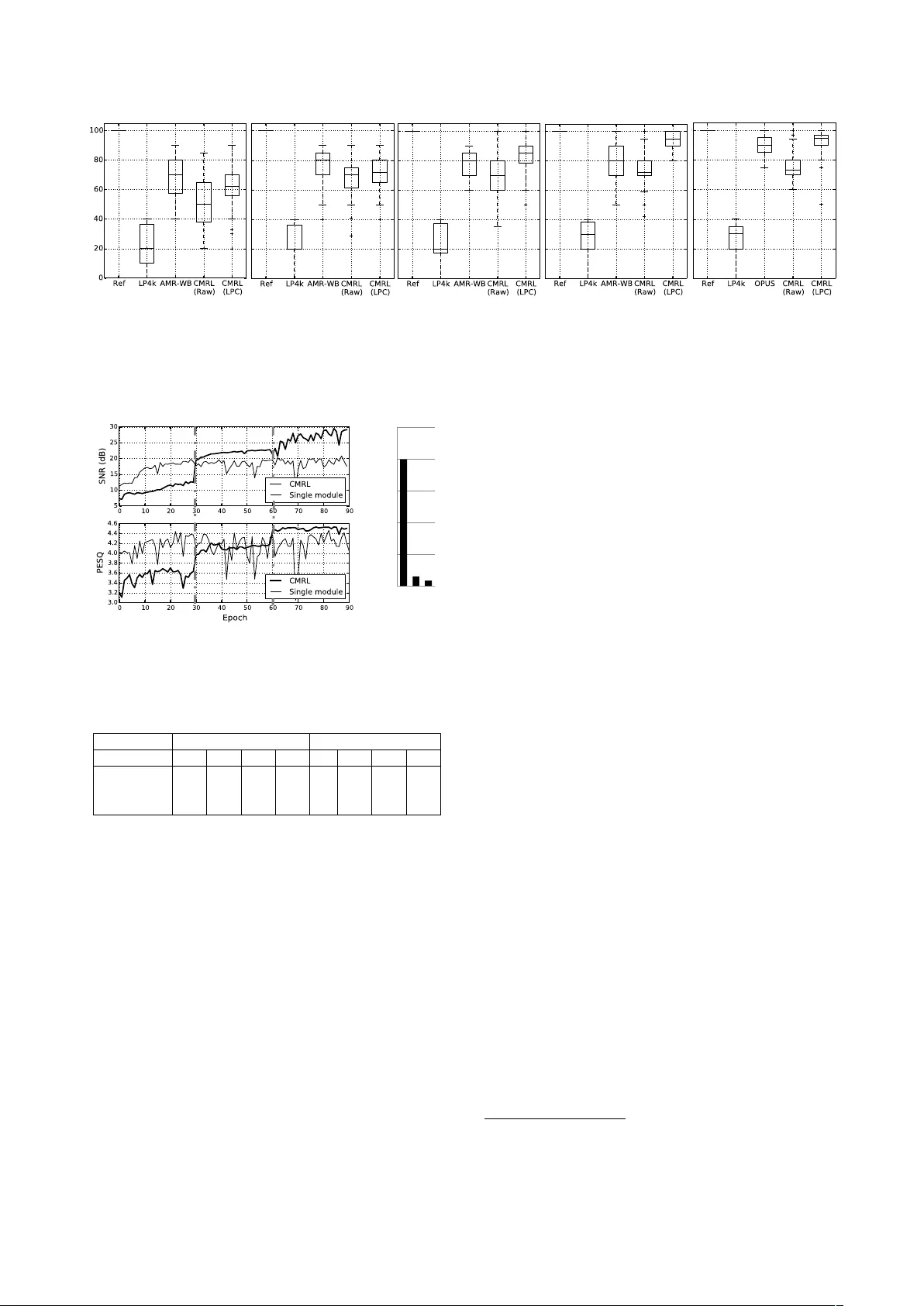
Cascaded Cr oss-Module Residual Learning towards Lightweight End-to-End Speech Coding Kai Zhen 1 , 2 , J ongmo Sung 3 , Mi Suk Lee 3 , Seungkwon Beack 3 , Minje Kim 1 , 2 1 Indiana Uni versity , School of Informatics, Computing, and Engineering, Bloomington, IN 2 Indiana Uni versity , Cogniti ve Science Program, Bloomington, IN 3 Electronics and T elecommunications Research Institute, Daejeon, South K orea zhenk@iu.edu, jmseong@etri.re.kr, lms@etri.re.kr, skbeack@etri.re.kr, minje@indiana.edu Abstract Speech codecs learn compact representations of speech signals to f acilitate data transmission. Many recent deep neural net- work (DNN) based end-to-end speech codecs achieve low bi- trates and high perceptual quality at the cost of model com- plexity . W e propose a cross-module residual learning (CMRL) pipeline as a module carrier with each module reconstructing the residual from its preceding modules. CMRL differs from other DNN-based speech codecs, in that rather than modeling speech compression problem in a single large neural network, it optimizes a series of less-complicated modules in a two-phase training scheme. The proposed method shows better objec- tiv e performance than AMR-WB and the state-of-the-art DNN- based speech codec with a similar network architecture. As an end-to-end model, it takes raw PCM signals as an input, but is also compatible with linear predictiv e coding (LPC), show- ing better subjective quality at high bitrates than AMR-WB and OPUS. The gain is achie v ed by using only 0.9 million trainable parameters, a significantly less comple x architecture than the other DNN-based codecs in the literature. Index T erms : speech coding, deep neural network, entropy coding, residual learning 1. Introduction Speech coding, where the encoder conv erts the speech signal into bitstreams and the decoder synthesizes reconstructed signal from receiv ed bitstreams, serves an important role for various purposes: to secure a v oice communication [1][2], to facilitate data transmission [3], etc. There ha ve been various conventional speech coding methodologies, including linear predictiv e cod- ing (LPC) [4], adaptive encoding [5], and perceptual weighting [6] among other domain specific knowledge about the speech signals, that are used to construct classic codecs, such as AMR- WB [7] and OPUS [8] with high perceptual quality . Since the last decade, data-driven approaches have vital- ized the use of deep neural networks (DNN) for speech cod- ing. A speech coding system can be formulated by DNN as an autoencoder (AE) with a code layer discretized by vector quantization (VQ) [9] or bitwise network techniques [10], etc. Many DNN methods [11][12] take inputs in time-frequency (T - F) domain from short time F ourier transform (STFT) or modi- fied discrete cosine transform (MDCT), etc. Recent DNN-based codecs [13][14][15][16] model speech signals in time domain directly without T -F transformation. They are referred to as end- to-end methods, yielding competitive performance comparing with current speech coding standards, such as AMR-WB [7]. While DNN serves a po werful parameter estimation paradigm, they are computationally expensi ve to run on smart devices. Many DNN-based codecs achie ve both lo w bitrates and high perceptual quality , two main targets for speech codecs [17][18][19], but with a high model complexity . A W aveNet based variational autoencoder (V AE) [16] outperforms other low bitrate codecs in the listening test, howev er , with 20 mil- lions parameters, a too big model for real-time processing in a resource-constrained device. Similarly , codecs built on Sam- pleRNN [20][21] can also be energy-intensi v e. Motiv ated by DNN based end-to-end codecs [14] and resid- ual cascading [22][23], this paper proposes a “cross-module” residual learning (CMRL) pipeline, which can lower the model complexity while maintaining a high perceptual quality and compression ratio. CMRL hosts a list of less-complicated end- to-end speech coding modules. Each module learns to re- cov er what is failed to be reconstructed by its preceding mod- ules. CMRL differs from other residual learning networks, e.g. ResNet [24], in that rather than adding identical short- cuts between layers, CMRL cascades residuals across a series of DNN modules. W e introduce a two-round model training scheme to train CMRL models. In addition, we also show that CMRL is compatible with LPC by having it as one of the mod- ules. W ith LPC coefficients being predicted, CMRL recovers the LPC residuals which, along with the LPC coefficients, syn- thesize the decoded speech signal at the receiv er side. The ev aluation of the propose method is threefold: ob- jectiv e measures, subjecti ve assessment and model complexity . Comparing with AMR-WB, OPUS, and the recently proposed end-to-end system [14], CMRL showed promising performance both in objecti ve and subjective quality assessments. As for complexity , CMRL contains only 0.9 million model parameters, significantly less complicated than the W aveNet based speech codec [16] and the end-to-end baseline [14]. 2. Model description Before introducing CMRL as a module carrier , we describe the component module to be hosted by CMRL. 2.1. The component module Recently , an end-to-end DNN speech codec (referred to as Kankanahalli-Net) has sho wn competitive performance compa- rable to one of the standards (AMR-WB) [14]. W e describe our component model deriv ed from Kankanahalli-Net that consists of bottleneck residual learning [24], soft-to-hard quantization [25], and sub-pixel conv olutional neural networks for upsam- pling [26]. Figure 1 depicts the component module. so# $ 0" 1" …" 0" 0$ 0$ …$ 1$ …$ …$ …$ …$ 0$ 1$ …$ 0$ clustering assignment entropy coding entropy decoding … (a). Raw PCM or LPC residual signal (f). decoded signal (b). bottle-neck blocks (b). bottle-neck blocks (c). softmax quantization (e). quantized code (d). entropy coding … Encoder Decoder … Down$ sampling$ … Up$ sampling$ (b). bottle-neck blocks (b). bottle-neck blocks Figure 1: A schematic diagram for the end-to-end speec h coding component module: some channel c hange steps ar e omitted. Figure 2: The interlacing-based upsampling pr ocess. 2.1.1. F our non-linear mapping types In the end-to-end speech codec, we tak e S = 512 time domain samples per frame, 32 of which are windo wed by the either left or right half of a Hann windo w and then o verlapped with the ad- jacent ones. This forms the input to the first 1-D con v olutional layer of C kernels, whose output is a tensor of size S × C . There are four types of non-linear transformations in volv ed in this fully con volutional network: downsampling, upsam- pling, channel changing, and residual learning. The do wnsam- pling operation reduces S do wn to S/ 2 by setting the stride d of the con volutional layer to be 2 , which turns an input e xample S × C into S/ 2 × C . The original dimension S is recov ered in the decoder with recently proposed sub-pixel conv olution [25], which forms the upsampling operation. The super -pixel con vo- lution is done by interlacing multiple feature maps to expand the size of the window (Figure 2). In our case, we interlace a pair of feature maps, and that is why in T able 1 the upsampling layer reduces the channels from 100 to 50 while recovers the original 512 dimensions from 256. In this work, to simplify the model architecture we hav e identical shortcuts only for cross-layer residual learning, while Kankanahalli-Net emplo ys them more frequently . Furthermore, inspired by recent work in source separation with dilated con- volutional neural network [27], we use a “bottleneck” residual learning block to further reduce the number of parameters. This can lower the amount of parameters, because the reduced num- ber of channels within the bottleneck residual learning block de- creases the depth of the kernels. See T able 1 for the size of our kernels. Like wise, the input S × 1 tensor is firstly conv erted to a S × C feature map, and then do wnsampled to S/ 2 × C . Even- tually , the code vector shrinks down to S/ 2 × 1 . The decoding process recov ers it back to a signal of size S × 1 , reversely . 2.1.2. Softmax quantization: The coded output from each encoder is still a real-valued vector of size S/ 2 . Softmax quantization [25] performs scalar quanti- zation by assigning each real value to the nearest representati v e (Figure 1 (c)). In the proposed system, softmax quantization maps the input scalar to one of the 32 clusters, or quantization lev els, which requires log 2 32 = 5 bits per dimension. Huffman coding further reduces the bitrate [28]. 2.2. The module carrier: CMRL Figure 3 shows the proposed cascaded cross-module residual learning (CMRL) process. In CMRL, each module does its best to reconstruct its input. The procedure in the i -th module is denoted as F ( x ( i ) ; W ( i ) ) , which estimates the input as ˆ x ( i ) . The input for the i -th module is defined as x ( i ) = x − i − 1 X j =1 ˆ x ( j ) , (1) where the first module takes the input speech signal, i.e., x (1) = x . The meaning is that each module learns to reconstruct the residual which is not recovered by its preceding modules. Note that module homogeneity is not required for CMRL: for exam- ple, the first module can be very shallow to just estimate the en velope of MDCT spectral structure while the following mod- ules may need more parameters to estimate the residuals. Each AE decomposes into the encoder and decoder parts: h ( i ) = F enc ( x ( i ) ; W ( i ) enc ) , ˆ x ( i ) = F dec ( h ( i ) ; W ( i ) dec ) , (2) where h ( i ) denotes the part of code generated by the i -th en- coder , and W ( i ) enc ∪ W ( i ) dec = W ( i ) . The encoding process : F or a gi ven input signal x , the en- coding process runs all N AE modules in a sequential order. Then, the bitstring is generated by taking the encoder outputs and concatenating them: h = h h (1) > , h (2) > , · · · , h ( N ) > i > . The decoding process : Once the bitstring is av ailable on the receiv er side, all the decoder parts of the modules, F dec ( x ( i ) ; W ( i ) dec ) ∀ N , run to produce the reconstructions which are added up to approximate the initial input signal with the global error defined as ˆ E x         N X i =1 ˆ x ( i ) ! . (3) 2.2.1. The two-r ound tr aining scheme Intra-module greedy training: W e provide a two-round train- ing scheme to make CMRL optimization tractable. The first round adopts a greedy training scheme, where each AE tries its best to minimize the error: arg min W ( i ) E ( x ( i ) ||F ( x ( i ) ; W ( i ) )) . The greedy training scheme echoes a divide-and-conquer man- ner , leading to an easier optimization for each module. The thick gray arro ws in Figure 3 sho w the flo w of the backpropaga- tion error to minimize the individual module error with respect to the module-specific parameter set W ( i ) . The 1 st module En co d er Dec o d e r Co d e Layer En co d er Dec o d e r Co d e Layer The 2 nd module En co d er Dec o d e r Co d e Layer The N th module ·· · AAACBnicZZDLSgMxFIYz3q23qks3wSK4KO2MCLoSQRcuFWwV2iKZzJkam8uQnBHL0L1Lt/oQ7sStr+Ez+BKmtQu1BwLf+ZP/cPLHmRQOw/AzmJqemZ2bX1gsLS2vrK6V1zeazuSWQ4Mbaex1zBxIoaGBAiVcZxaYiiVcxb2T4f3VPVgnjL7EfgYdxbpapIIz9FKzzROD7qZcCWvhqOgkRGOokHGd35S/2onhuQKNXDLnWlGYYadgFgWXMCi1cwcZ4z3WhZZHzRS4TjHadkB3vJLQ1Fh/NNKR+ttRMOVcX8VV6kExvK3SWHnbEN3f0ZgedgqhsxxB85/JaS4pGjr8K02EBY6y74FxK/xylN8yyzj6RErtkbGoN5zv6kroO+gJVT+1JovNQz2BtOYAByWfTvQ/i0lo7tWisBZd7FeOj8Y5LZAtsk12SUQOyDE5I+ekQTi5I0/kmbwEj8Fr8Ba8/zydCsaeTfKngo9vqEeYhg== AAACBnicZZDLSgMxFIYz3q23qks3wSK4KO2MCLoSQRcuFWwV2iKZzJkam8uQnBHL0L1Lt/oQ7sStr+Ez+BKmtQu1BwLf+ZP/cPLHmRQOw/AzmJqemZ2bX1gsLS2vrK6V1zeazuSWQ4Mbaex1zBxIoaGBAiVcZxaYiiVcxb2T4f3VPVgnjL7EfgYdxbpapIIz9FKzzROD7qZcCWvhqOgkRGOokHGd35S/2onhuQKNXDLnWlGYYadgFgWXMCi1cwcZ4z3WhZZHzRS4TjHadkB3vJLQ1Fh/NNKR+ttRMOVcX8VV6kExvK3SWHnbEN3f0ZgedgqhsxxB85/JaS4pGjr8K02EBY6y74FxK/xylN8yyzj6RErtkbGoN5zv6kroO+gJVT+1JovNQz2BtOYAByWfTvQ/i0lo7tWisBZd7FeOj8Y5LZAtsk12SUQOyDE5I+ekQTi5I0/kmbwEj8Fr8Ba8/zydCsaeTfKngo9vqEeYhg== AAACBnicZZDLSgMxFIYz3q23qks3wSK4KO2MCLoSQRcuFWwV2iKZzJkam8uQnBHL0L1Lt/oQ7sStr+Ez+BKmtQu1BwLf+ZP/cPLHmRQOw/AzmJqemZ2bX1gsLS2vrK6V1zeazuSWQ4Mbaex1zBxIoaGBAiVcZxaYiiVcxb2T4f3VPVgnjL7EfgYdxbpapIIz9FKzzROD7qZcCWvhqOgkRGOokHGd35S/2onhuQKNXDLnWlGYYadgFgWXMCi1cwcZ4z3WhZZHzRS4TjHadkB3vJLQ1Fh/NNKR+ttRMOVcX8VV6kExvK3SWHnbEN3f0ZgedgqhsxxB85/JaS4pGjr8K02EBY6y74FxK/xylN8yyzj6RErtkbGoN5zv6kroO+gJVT+1JovNQz2BtOYAByWfTvQ/i0lo7tWisBZd7FeOj8Y5LZAtsk12SUQOyDE5I+ekQTi5I0/kmbwEj8Fr8Ba8/zydCsaeTfKngo9vqEeYhg== AAACBnicZZDLSgMxFIYz3q23qks3wSK4KO2MCLoSQRcuFWwV2iKZzJkam8uQnBHL0L1Lt/oQ7sStr+Ez+BKmtQu1BwLf+ZP/cPLHmRQOw/AzmJqemZ2bX1gsLS2vrK6V1zeazuSWQ4Mbaex1zBxIoaGBAiVcZxaYiiVcxb2T4f3VPVgnjL7EfgYdxbpapIIz9FKzzROD7qZcCWvhqOgkRGOokHGd35S/2onhuQKNXDLnWlGYYadgFgWXMCi1cwcZ4z3WhZZHzRS4TjHadkB3vJLQ1Fh/NNKR+ttRMOVcX8VV6kExvK3SWHnbEN3f0ZgedgqhsxxB85/JaS4pGjr8K02EBY6y74FxK/xylN8yyzj6RErtkbGoN5zv6kroO+gJVT+1JovNQz2BtOYAByWfTvQ/i0lo7tWisBZd7FeOj8Y5LZAtsk12SUQOyDE5I+ekQTi5I0/kmbwEj8Fr8Ba8/zydCsaeTfKngo9vqEeYhg== Res i d ual s ignal Res i d ual s ignal x (2) = x  ˆ x (1) AAACMnicbZDLbhMxFIY9KdAQLk3Lko2VCCldkMykldoNUgVdsAwSSStlQuRxziRufBnZZ1Cj0ex5GlZI7auUHWLLC7DDuSwg5UiWPv/n/Dr2n2RSOAzDu6Cy8+Dho93q49qTp8+e79X3DwbO5JZDnxtp7GXCHEihoY8CJVxmFphKJFwk83fL/sVnsE4Y/REXGYwUm2qRCs7QS+N6I06uPxWt7mFJ31DP9DWNZwwLj6XXo8OyNq43w3a4Knofog00yaZ64/rveGJ4rkAjl8y5YRRmOCqYRcEllLU4d5AxPmdTGHrUTIEbFau/lPSVVyY0NdYfjXSl/u0omHJuoRI/qRjO3HZvKf6vN8wxPR0VQmc5gubrRWkuKRq6DIZOhAWOcuGBcSv8WymfMcs4+vhq8cpYdPrO3zpK6CuYC9U5tyZLzHVnAmnbAZY+q2g7mfsw6Lajo3b3w3Hz7O0mtSp5SRqkRSJyQs7Ie9IjfcLJF/KV3JDb4FvwPfgR/FyPVoKN5wX5p4JffwAUNajy x (1) = x AAACIHicbVDLSgMxFM34rPU16tJNsAi6aWeqoBuhqAuXCrYV2loy6Z02No8hyYhl6J+4EvRb3IlL/RN3prULXwcCJ+fcw72cKOHM2CB486amZ2bn5nML+cWl5ZVVf229ZlSqKVSp4kpfRcQAZxKqllkOV4kGIiIO9ah/MvLrt6ANU/LSDhJoCdKVLGaUWCe1fb8Z3V1nO+HuEB9hx/NtvxAUgzHwXxJOSAFNcN72P5odRVMB0lJOjGmEQWJbGdGWUQ7DfDM1kBDaJ11oOCqJANPKxpcP8bZTOjhW2j1p8Vj9nsiIMGYgIjcpiO2Z395I/M9rpDY+bGVMJqkFSb8WxSnHVuFRDbjDNFDLB44Qqpm7FdMe0YRaV1a+OQ5mpapxv5Jg8gb6TJROtUoidVfqQFw0YIeuq/B3M39JrVwM94rli/1C5XjSWg5toi20g0J0gCroDJ2jKqLoFt2jR/TkPXjP3ov3+jU65U0yG+gHvPdPzvyiMQ== h (1) AAACGHicbVDLTgIxFO34RHyhLt1MJCa4gRk00SVRFy4xkUcEJJ1yByp9TNqOkUz4C1cm+i3ujFt3foo7y2Oh4EmanJ5zT3p7gohRbTzvy1lYXFpeWU2tpdc3Nre2Mzu7VS1jRaBCJJOqHmANjAqoGGoY1CMFmAcMakH/YuTXHkBpKsWNGUTQ4rgraEgJNla6bQa9uyTnHw3T7UzWy3tjuPPEn5IsmqLcznw3O5LEHIQhDGvd8L3ItBKsDCUMhulmrCHCpI+70LBUYA66lYw3HrqHVum4oVT2COOO1d+JBHOtBzywkxybnp71RuJ/XiM24VkroSKKDQgyeSiMmWukO/q+26EKiGEDSzBR1O7qkh5WmBhbUro5DiaFira3AqfiHvqUFy6VjAL5WOhAmNdghrYrf7aZeVIt5v3jfPH6JFs6n7aWQvvoAOWQj05RCV2hMqogggR6Qi/o1Xl23px352MyuuBMM3voD5zPH2uhoAE= h (2) AAACGHicbVDLTgIxFO34RHyhLt1MJCa4gRk00SVRFy4xkUcEJJ1yByp9TNqOkUz4C1cm+i3ujFt3foo7y2Oh4EmanJ5zT3p7gohRbTzvy1lYXFpeWU2tpdc3Nre2Mzu7VS1jRaBCJJOqHmANjAqoGGoY1CMFmAcMakH/YuTXHkBpKsWNGUTQ4rgraEgJNla6bQa9uyRXPBqm25msl/fGcOeJPyVZNEW5nfludiSJOQhDGNa64XuRaSVYGUoYDNPNWEOESR93oWGpwBx0KxlvPHQPrdJxQ6nsEcYdq78TCeZaD3hgJzk2PT3rjcT/vEZswrNWQkUUGxBk8lAYM9dId/R9t0MVEMMGlmCiqN3VJT2sMDG2pHRzHEwKFW1vBU7FPfQpL1wqGQXysdCBMK/BDG1X/mwz86RazPvH+eL1SbZ0Pm0thfbRAcohH52iErpCZVRBBAn0hF7Qq/PsvDnvzsdkdMGZZvbQHzifP21PoAI= h ( N ) AAACGHicbVDLSgMxFM34rPVVdelmsAi6aWeqoMuiLlxJBacV21oy6R0bm8eQZMQy9C9cCfot7sStOz/Fneljoa0HAifn3ENuThgzqo3nfTkzs3PzC4uZpezyyuraem5js6ploggERDKprkOsgVEBgaGGwXWsAPOQQS3sng782gMoTaW4Mr0YmhzfCRpRgo2Vbhph5zbdu9jvZ1u5vFfwhnCniT8meTRGpZX7brQlSTgIQxjWuu57sWmmWBlKGPSzjURDjEkX30HdUoE56GY63Ljv7lql7UZS2SOMO1R/J1LMte7x0E5ybDp60huI/3n1xETHzZSKODEgyOihKGGuke7g+26bKiCG9SzBRFG7q0s6WGFibEnZxjCYFgNtb0VOxT10KS+eKRmH8rHYhqigwfRtV/5kM9OkWir4B4XS5WG+fDJuLYO20Q7aQz46QmV0jiooQAQJ9IRe0Kvz7Lw5787HaHTGGWe20B84nz+cV6Ae ˆ x (1) F ( x (1) ; W (1) ) AAACT3icZZDfahQxFMYzW7Xt+m/VS2+Ci7CFsjtTCwqCFCrijVDB7RY665JkznTTTSZDcqbtEuapfBIve6uXPoB3YmZ3Lqw9EPidk+87JB8vlXQYx9dRZ+PO3XubW9vd+w8ePnrce/L02JnKChgLo4w94cyBkgWMUaKCk9IC01zBhC8Om/vJBVgnTfEFlyVMNTsrZC4FwzCa9T6lc4Y+5Vf1Vz9IdupUQY7MWnNJU81wLpjyH+pByo3Kmr6RrpX127WCcz9pzTuzXj8exquityFpoU/aOpr1fqWZEZWGAoVizp0mcYlTzyxKoaDuppWDkokFO4PTgAXT4KZ+9e2avgyTjObGhlMgXU3/dXimnVtqvksDNE/dpVwHW4Pu5mrM30y9LMoKoRDrzXmlKBrahEYzaUGgWgZgwsrwOCrmzDKBIdpuujL60diFbqRlcQ4LqUfvrSm5uRplkA8dYN0N6ST/Z3EbjveGyavh3uf9/sG7Nqct8py8IAOSkNfkgHwkR2RMBPlGrskP8jP6Hv2O/nRaaSdq4Rm5UZ3tvwlTs7k= ˆ x (2) F ( x (2) ; W (2) ) AAACT3icZZDNahsxFIU17l/i/rnpshtRU3Ag2DNuoYVCCLSUbgop1HEg4xpJcydWLI0G6U4SI+ap+iRdZtsu+wDdlWrsWTTNBcF3r865SIeXSjqM46uoc+v2nbv3tra79x88fPS492TnyJnKCpgIo4w95syBkgVMUKKC49IC01zBlC/fNffTc7BOmuILrkqYaXZayFwKhmE0731KFwx9yi/rr34w3q1TBTkya80FTTXDhWDKf6gHKTcqa/pGulHWbzcKzv20Ne/Oe/14GK+L3oSkhT5p63De+5VmRlQaChSKOXeSxCXOPLMohYK6m1YOSiaW7BROAhZMg5v59bdr+iJMMpobG06BdD391+GZdm6l+R4N0Dx1j3IdbA2666sxfzPzsigrhEJsNueVomhoExrNpAWBahWACSvD46hYMMsEhmi76droRxMXupGWxRkspR69t6bk5nKUQT50gHU3pJP8n8VNOBoPk5fD8edX/YP9Nqct8ow8JwOSkNfkgHwkh2RCBPlGrsgP8jP6Hv2O/nRaaSdq4Sm5Vp3tvw6Ds7w= ˆ x ( N ) F ( x ( N ) ; W ( N ) ) AAACT3icZZBdaxNBFIZnU7Vt/Ip62ZvBIKRQkt0qVBCkoIg3SgXTFLoxzMyebcbMxzJz1jYs+6v8JV72tl76A7wTZ5O9sPbAwHPOvO9h5uWFkh7j+DLqbNy6fWdza7t79979Bw97jx4fe1s6AWNhlXUnnHlQ0sAYJSo4KRwwzRVM+OJNcz/5Bs5Laz7jsoCpZmdG5lIwDKNZ70M6Z1il/KL+Ug0+7tapghyZc/acpprhXDBVvasHKbcqa/pGulbWr9YKzqtJa96d9frxMF4VvQlJC33S1tGs9yvNrCg1GBSKeX+axAVOK+ZQCgV1Ny09FEws2BmcBjRMg59Wq2/X9FmYZDS3LhyDdDX911Ex7f1S8z0aoHnqHuU62Br011dj/nJaSVOUCEasN+elomhpExrNpAOBahmACSfD46iYM8cEhmi76cpYjcY+dCMtzVdYSD1662zB7cUog3zoAetuSCf5P4ubcLw/TJ4P9z+96B++bnPaIjvkKRmQhByQQ/KeHJExEeQ7uSRX5Gf0I/od/em00k7UwhNyrTrbfwGfw7QQ E ( x (1) || ˆ x (1) ) AAACL3icZZDPShxBEMZ7TDRmNWaNx1waF2EFsztjBHMKQhLI0YCrgrMu3b01bmf7z9BdIy7jPEWexGOu+hAhl5BryEukd3YPUQsKfvV1f0Xx8VxJj3H8M1p48nRx6dny88bK6ou1l831V8feFk5AT1hl3SlnHpQ00EOJCk5zB0xzBSd8/GH6fnIJzktrjnCSQ1+zCyMzKRgGadB8k9Y7Sq4KqFLB1Kd2yq/Oy3ayXV1fpyOGZZirmbA9aLbiTlwXfQzJHFpkXoeD5t90aEWhwaBQzPuzJM6xXzKHUiioGmnhIWdizC7gLKBhGny/rE+q6FZQhjSzLrRBWqv/O0qmvZ9ovkMDaIajHcp1sE3R31+N2bt+KU1eIBgx25wViqKl01DoUDoQqCYBmHAyHEfFiDkmMETXSGtj2e35MHW1NF9hLHX3o7M5t1fdIWQdD1g1QjrJwywew/FuJ3nb2f2y1zp4P89pmbwmm6RNErJPDshnckh6RJBv5Du5JXfRTfQj+hX9nn1diOaeDXKvoj//AI97qKo= E ( x (2) || ˆ x (2) ) AAACL3icZZDfShtBFMZnrbU2tprWy94MhkIEm+ymgr0qQlvopQWjghvDzOSsGTN/lpmzxbDuU/RJvOytPkTpTelt6Ut0ssmF1gMHfueb+Q6Hj+dKeozjn9HSo+XHK09WnzbWnj1f32i+eHnkbeEE9IVV1p1w5kFJA32UqOAkd8A0V3DMJx9m78dfwXlpzSFOcxhodm5kJgXDIA2bb9J6R8lVAVUqmPrUTvnlWdnubVdXV+mYYRnmai5sD5utuBPXRR9CsoAWWdTBsPk3HVlRaDAoFPP+NIlzHJTMoRQKqkZaeMiZmLBzOA1omAY/KOuTKvo6KCOaWRfaIK3Vu46Sae+nmu/QAJrheIdyHWwz9PdXY/ZuUEqTFwhGzDdnhaJo6SwUOpIOBKppACacDMdRMWaOCQzRNdLaWHb7PkxdLc0FTKTufnQ25/ayO4Ks4wGrRkgn+T+Lh3DU6yRvO70vu63994ucVskrskXaJCF7ZJ98JgekTwT5Rr6TG3IbXUc/ol/R7/nXpWjh2ST3KvrzD5LMqKw= E ( x ( N ) || ˆ x ( N ) ) AAACL3icZZDPahRBEMZ7EmPiJupGj14al8AG4u5MDMSTBKLgSSJkk0Bms3T31mQ723+G7hrJMpmn8Ek8etWHkFyCV/El7J3dQ/4UFPzq6/6K4uO5kh7j+DpaWHy09Hh55Uljde3ps+fN9RdH3hZOQE9YZd0JZx6UNNBDiQpOcgdMcwXHfLw/fT/+Cs5Law5xkkNfs3MjMykYBmnQfJPWO0quCqhSwdTHdsovz8r2583q6iodMSzDXM2EzUGzFXfiuuhDSObQIvM6GDT/pUMrCg0GhWLenyZxjv2SOZRCQdVICw85E2N2DqcBDdPg+2V9UkU3gjKkmXWhDdJave0omfZ+ovkWDaAZjrYo18E2RX93NWbv+qU0eYFgxGxzViiKlk5DoUPpQKCaBGDCyXAcFSPmmMAQXSOtjWW358PU1dJcwFjq7gdnc24vu0PIOh6waoR0kvtZPISj7U7ytrP9Zae1936e0wp5RV6TNknILtkjn8gB6RFBvpEf5Cf5FX2Pfkc30Z/Z14Vo7nlJ7lT09z/vqKjk x ( N ) = x  P N  1 i =1 ˆ x ( i ) AAACUnicbVLLThsxFHUCLTTQNtBlN1YjpLAgmaFIsEFClEVXCKQGkDIh8jh3iIkfI/sOIrLmf/gaVkjQT2lXOCELXleydHwesn3kNJfCYRT9rVTn5j98XFj8VFta/vzla31l9cSZwnLocCONPUuZAyk0dFCghLPcAlOphNN09Guin16BdcLoPzjOoafYhRaZ4AwD1a/vJ+n1uW8erpd0lwZMN6hPHLciR4djCTRxhep7sRuX5/5wIy5LmgwZ+mANRFOsl7V+vRG1ounQtyCegQaZzVG//i8ZGF4o0Mglc64bRzn2PLMouISylhQOcsZH7AK6AWqmwPX89K0lXQvMgGbGhqWRTtnnCc+Uc2OVBqdiOHSvtQn5ntYtMNvpeaHzAkHzp4OyQlI0dFIcHQgLHOU4ABb6CXelfMgs4xjqrSXToG93XNi1ldCXMBKqfWBNnprr9gCylgMsQ1fx62begpPNVvyztXm81djbn7W2SL6TH6RJYrJN9shvckQ6hJMbckvuyUPlrvK/Gn7Jk7VamWW+kRdTXX4ErwazxA== BP fo r BP fo r W ( N ) AAACIXicbVDLSsNAFJ34tr6qLt0Ei1A3TVIFXYq6cCUK1gptLZPJTTt2HmFmopaQT3El6Le4E3fil7hzWrtQ64GBM+fewz2cMGFUG99/dyYmp6ZnZufmCwuLS8srxdW1Sy1TRaBGJJPqKsQaGBVQM9QwuEoUYB4yqIe9o8G8fgtKUykuTD+BFscdQWNKsLFSu7ja5Nh0wzCr59dZ+XQ7L7SLJb/iD+GOk2BESmiEs3bxsxlJknIQhjCsdSPwE9PKsDKUMMgLzVRDgkkPd6BhqcAcdCsbRs/dLatEbiyVfcK4Q/WnI8Nc6z4P7eYgqP47G4j/zRqpifdbGRVJakCQ70Nxylwj3UEPbkQVEMP6lmCiqM3qki5WmBjbVqE5NGZeTdufx6m4gR7l3rGSSSjvvQjiigaT266Cv82Mk8tqJdipVM93SweHo9bm0AbaRGUUoD10gE7QGaohgu7QA3pCz86j8+K8Om/fqxPOyLOOfsH5+AIuQ6OI W (2) AAACIXicbVC7TgJBFJ3FF+ILtLTZSEywgV000ZKohaUmIiSAZHa4CyPz2MzMqmSzn2Jlot9iZ+yMX2LngBSKnmSSM+fek3tygohRbTzv3cnMzS8sLmWXcyura+sb+cLmlZaxIlAnkknVDLAGRgXUDTUMmpECzAMGjWB4Mp43bkFpKsWlGUXQ4bgvaEgJNlbq5gttjs0gCJJGep2UqntprpsvemVvAvcv8aekiKY47+Y/2z1JYg7CEIa1bvleZDoJVoYSBmmuHWuIMBniPrQsFZiD7iST6Km7a5WeG0plnzDuRP3pSDDXesQDuzkOqmdnY/G/WSs24VEnoSKKDQjyfSiMmWukO+7B7VEFxLCRJZgoarO6ZIAVJsa2lWtPjEmlru2vwqm4gSHllVMlo0DeV3oQljWY1Hblzzbzl1xVy/5+uXpxUKwdT1vLom20g0rIR4eohs7QOaojgu7QA3pCz86j8+K8Om/fqxln6tlCv+B8fAH/LKNs BP fo r W (1) AAACIXicbVDLSsNAFJ34rPHV6tJNsAh10yZV0GVRFy4VrC20tUymNzp2HmFmopaQT3El6Le4E3fil7hzGrvwdWDgzLn3cA8njBnVxvffnKnpmdm5+cKCu7i0vLJaLK2da5koAk0imVTtEGtgVEDTUMOgHSvAPGTQCoeH43nrBpSmUpyZUQw9ji8FjSjBxkr9YqnLsbkKw7SVXaSVYDtz+8WyX/VzeH9JMCFlNMFJv/jRHUiScBCGMKx1J/Bj00uxMpQwyNxuoiHGZIgvoWOpwBx0L82jZ96WVQZeJJV9wni5+t2RYq71iId2cxxU/56Nxf9mncRE+72UijgxIMjXoShhnpHeuAdvQBUQw0aWYKKozeqRK6wwMbYtt5sb01pT21+NU3ENQ8prR0rGobyrDSCqajCZ7Sr43cxfcl6vBjvV+uluuXEwaa2ANtAmqqAA7aEGOkYnqIkIukX36BE9OQ/Os/PivH6tTjkTzzr6Aef9E/1+o2s= ˆ E x         N X i =1 ˆ x ( N ) ! AAACT3icZZDNbhMxFIU94a8NfwGWbCwipFSqkpmCBBtQJUBiQ1Uk0laq08j23JmY2DMj+w5KZOapeBKW3cKSB2CHcKazoPRItj4f33t1dUSllcM4Po96167fuHlra7t/+87de/cHDx4eubK2Eqay1KU9EdyBVgVMUaGGk8oCN0LDsVi+2fwffwHrVFl8wnUFM8PzQmVKcgzWfPCBtTO8hbRhC46eSa7fNUxDhiMmVkyoPP/a3a42c69eJc3ZwUWtWDVnfnSw0zCr8gXuzAfDeBy3olch6WBIOh3OB79YWsraQIFSc+dOk7jCmecWldTQ9FntoOJyyXM4DVhwA27m25Ub+jQ4Kc1KG06BtHX/7fDcOLc2YpcGMBwXu1SY0LZBd3k0Zi9nXhVVjVDIi8lZrSmWdBMaTZUFiXodgEurwnJULrjlEkO0fdY2+snUhdfEqOIzLJWZvLVlJcrVJIVs7ACbfkgn+T+Lq3C0N06ejfc+Ph/uv+5y2iKPyRMyIgl5QfbJe3JIpkSSb+Sc/CA/o+/R7+hPryvtRR08IpfU2/4Lx0e1Sw== 1 st Ro u n d Ba c kp r o p a g a t io n F l o w Re sid u a l Si g n a l s F lo w 2 nd Ro u n d Ba c kp r o p a g a t io n F l o w 1 st Ro u n d E r r o r F u n c t i o n 2 nd Ro u n d E r r o r F u n ct i o n E ( x ( N ) || ˆ x ( N ) ) AAACL3icZZDPahRBEMZ7EmPiJupGj14al8AG4u5MDMSTBKLgSSJkk0Bms3T31mQ723+G7hrJMpmn8Ek8etWHkFyCV/El7J3dQ/4UFPzq6/6K4uO5kh7j+DpaWHy09Hh55Uljde3ps+fN9RdH3hZOQE9YZd0JZx6UNNBDiQpOcgdMcwXHfLw/fT/+Cs5Law5xkkNfs3MjMykYBmnQfJPWO0quCqhSwdTHdsovz8r2583q6iodMSzDXM2EzUGzFXfiuuhDSObQIvM6GDT/pUMrCg0GhWLenyZxjv2SOZRCQdVICw85E2N2DqcBDdPg+2V9UkU3gjKkmXWhDdJave0omfZ+ovkWDaAZjrYo18E2RX93NWbv+qU0eYFgxGxzViiKlk5DoUPpQKCaBGDCyXAcFSPmmMAQXSOtjWW358PU1dJcwFjq7gdnc24vu0PIOh6waoR0kvtZPISj7U7ytrP9Zae1936e0wp5RV6TNknILtkjn8gB6RFBvpEf5Cf5FX2Pfkc30Z/Z14Vo7nlJ7lT09z/vqKjk ˆ E x         N X i =1 ˆ x ( N ) ! AAACT3icZZDNbhMxFIU94a8NfwGWbCwipFSqkpmCBBtQJUBiQ1Uk0laq08j23JmY2DMj+w5KZOapeBKW3cKSB2CHcKazoPRItj4f33t1dUSllcM4Po96167fuHlra7t/+87de/cHDx4eubK2Eqay1KU9EdyBVgVMUaGGk8oCN0LDsVi+2fwffwHrVFl8wnUFM8PzQmVKcgzWfPCBtTO8hbRhC46eSa7fNUxDhiMmVkyoPP/a3a42c69eJc3ZwUWtWDVnfnSw0zCr8gXuzAfDeBy3olch6WBIOh3OB79YWsraQIFSc+dOk7jCmecWldTQ9FntoOJyyXM4DVhwA27m25Ub+jQ4Kc1KG06BtHX/7fDcOLc2YpcGMBwXu1SY0LZBd3k0Zi9nXhVVjVDIi8lZrSmWdBMaTZUFiXodgEurwnJULrjlEkO0fdY2+snUhdfEqOIzLJWZvLVlJcrVJIVs7ACbfkgn+T+Lq3C0N06ejfc+Ph/uv+5y2iKPyRMyIgl5QfbJe3JIpkSSb+Sc/CA/o+/R7+hPryvtRR08IpfU2/4Lx0e1Sw== Figure 3: Cr oss-module r esidual learning pipeline Cross-module finetuning: The greedy training scheme ac- cumulates module-specific error , which the earlier modules do not have a chance to reduce, thus leading to a suboptimal re- sult. Hence, the second-round cross-module finetuning follows to further improv e the performance by reducing the total error: arg min W (1) ··· W ( N ) ˆ E x         N X i =1 F  x ( i ) ; W ( i )  ! . (4) During the finetuing step, we first (a) initialize the parameters of each module with those estimated from the greedy training step (b) perform cascaded feedforward on all the modules sequen- tially to calculate the total estimation error in (3) (c) backprop- agate the error to update parameters in all modules altogether (thin black arrows in Figure 3). Aside from the total recon- struction error (3), we inherit Kankanahalli-Net’ s other regu- larization terms, i.e., perceptual loss, quantization penalty , and entropy regularizer . 2.3. Bitrate and entropy coding The bitrate is calculated from the concatenated bitstrings from all modules in CMRL. Each encoder module produces S/d quantized symbols from the softmax quantization process (Fig- ure 1 (e)), where the stride size d divides the input dimensional- ity . Let c ( i ) be the av erage bit length per symbol after Huffman coding in the i -th module. Then, c ( i ) S/d stands for the bits per frame. By dividing the frame rate, ( S − o ) /f , where o and f denote the overlap size in samples and the sampling rate, re- spectiv ely , the bitrates per module add up to the total bitrate: ξ LPC + P N i =1 f cS ( S − o ) d , where the overhead to transmit LPC co- efficients is ξ lpc =2.4kbps, which is 0 for the case with raw PCM signals as the input. By having the entropy control scheme proposed in Kankanahalli-Net as the baseline to keep a specific bitrate, we further enhance the coding efficiency by employing the Huff- man coding scheme on the vectors. Aside from encoding each symbol (i.e., the softmax result) separately , encoding short se- quences can further le verage the temporal correlation in the se- ries of quantized symbols, especially when the entropy is al- ready lo w [29] [30]. W e found that encoding a short symbol se- quence of adjacent symbols, i.e., two symbols, can lower do wn the av erage bit length further in the lo w bitrates. 3. Experiments W e first show that for the raw PCM input CMRL outperforms AMR-WB and Kankanahalli-Net in terms of objectiv e metrics in the experimental setup proposed in [14], where the use of LPC was not tested. Therefore, for the subjective quality , we perform MUSHRA tests [31] to show that CMRL with an LPC T able 1: Ar chitectur e of the component module as in F igur e 1. Input and output tensors sizes are r epr esented by (width, chan- nel), while the kernel shape is (width, in channel, out c hannel). Layer Input shape Kernel shape Output shape Change channel (512, 1) (9, 1, 100) (512, 100) 1st bottleneck (512, 100) (9, 100, 20) # × 2 (9, 20, 20) (9, 20, 100) (512, 100) Downsampling (512, 100) (9, 100, 100) (256, 100) 2nd bottleneck (256, 100) (9, 100, 20) # × 2 (9, 20, 20) (9, 20, 100) (256, 100) Change channel (256, 100) (9, 100, 1) (256, 1) Change channel (256, 1) (9, 1, 100) (256, 100) 1st bottleneck (256, 100) (9, 100, 20) # × 2 (9, 20, 20) (9, 20, 100) (256, 100) Upsampling (256, 100) (9, 100, 100) (512, 50) 2nd bottleneck (512, 50) (9, 50, 20) # × 2 (9, 20, 20) (9, 20, 50) (512, 50) Change channel (512, 50) (9, 50, 1) (512, 1) residual input works better than AMR-WB and OPUS at high bitrates. 3.1. Experimental setup 300 and 50 speakers are randomly selected from TIMIT [32] training and test datasets, respectiv ely . W e consider two types of inputs in time-domain: ra w PCM and LPC residuals. For the raw PCM input, the data is normalized to have a unit vari- ance, and then directly fed to the model. For the LPC residual input, we conduct a spectral en velope estimation on the ra w sig- nals to get LPC residuals and corresponding coefficients. The LPC residuals are modeled by the proposed end-to-end CMRL pipeline, while the LPC coefficients are quantized and sent di- rectly to the recei ver side at 2.4 kbps. The decoding process re- cov ers the speech signal based on the LPC synthesis procedure using the LPC coefficients and the decoded residual signals. W e consider four bitrate cases: 8.85 kbps, 15.85 kbps, 19.85 kbps and 23.85 kbps. All con volutional layers in CMRL use 1-D k ernel with the size of 9 and the Leaky Relu activ ation. CMRL hosts two modules: each module is with the topology as in T able 1. Each residual learning block contains two bottle- neck structures with the dilation rate of 1 and 2. Note that for the lowest bitrate case, the second encoder downsamples each window to 128 symbols. The learning rate is 0.0001 to train the first module, and 0.00002 for the second module. Finetuning uses 0.00002 as the learning rate, too. Each window contains 512 samples with the ov erlap size of 32. W e use Adam opti- mizer [33] with the batch size of 128 frames. Each module is trained for 30 epochs follo wed by finetuning until the entropy is (a) 8.85kbps (b) 15.85kbps (c) 19.85kbps (d) 23.85kbps (e) 23.85kbps Figure 4: MUSHRA test r esults. F r om (a) to (d): the performance of CMRL on raw and LPC residual input signals compar ed against AMR-WB at dif fer ent bitr ates. (e) An additional test shows that the performance of CMRL with the LPC input competes with OPUS, which is known to outperform AMR-WB in 23.85kbps. 1 st module training 2 nd module training fine-tuning (a) 0 5 10 15 20 25 WaveNet K-Net CMRL Model parameters (million) 0.9$ 1.5$ 20$ (b) Figure 5: (a) SNR and PESQ per epoch (b) model complexity T able 2: SNR and PESQ scores on r aw PCM test signals. Metrics SNR (dB) PESQ Bitrate (kbps) 8.85 15.85 19.85 23.85 8.85 15.85 19.85 23.85 AMR-WB 9.82 11.93 12.46 12.73 3.41 3.99 4.09 4.13 K-Net - - - - 3.63 4.13 4.22 4.30 CMRL 13.45 16.35 17.18 17.33 3.69 4.21 4.34 4.42 within the target range. 3.2. Objective test W e ev aluate 500 decoded utterances in terms of SNR and PESQ with wide band e xtension (P862.2) [34]. Figure 5 (a) sho ws the effecti v eness of CMRL against a system with a single module in terms of SNR and PESQ values per epoch. The single mod- ule is with three more bottleneck blocks and twice more codes for a fair comparison. It is trained for 90 epochs with other hy- perparameters are unaltered. For both SNR and PESQ, the plot shows a noticeable performance jump as the second module is included, followed by another jump by finetuning. T able 2 compares CMRL with AMR-WB and Kankanahalli-Net at four bitrates for the raw PCM input case. CMRL achieves both higher SNR and PESQ at all four bitrate cases. Note that the SNR for CMRL at 8.85 kbps is greater than AMR-WB at 23.85 kbps. CMRL also gi ves a better PESQ score at 15.85 kbps than AMR-WB at 23.85 kbps. 3.3. Subject test Figure 4 sho ws MUSHRA test results done by six audio experts on 10 decoded test samples randomly selected with gender eq- uity . At 19.85 kbps and 23.85 kbps, CMRL with LPC residual inputs outperforms AMR-WB. At lo wer bitrates though, AMR- WB starts to work better . CMRL on raw PCM is found less fa vored by listeners. W e also compare CMRL with OPUS in the high bitrate where OPUS is known to perform well, and find that CMRL slightly outperforms OPUS 1 . 3.4. Model complexity The cross-module residual learning simplifies the topology of each component module. Hence, CMRL has less than 5% of the model parameters compared to the W av eNet based codec [16], and outperforms Kankanahalli-Net with 40% less model parameters. Figure 5 (b) summarizes the comparison. 4. Conclusion In this work, we demonstrated that CMRL as a lightweight model carrier for DNN based speech codecs can compete with the industrial standards. By cascading two end-to-end mod- ules, CMRL achiev ed a higher PESQ score at 15.85 kbps than AMR-WB at 23.85 kbps. W e also showed that CMRL can con- sistently outperform a state-of-the-art DNN codec in terms of PESQ. CMRL is compatible with LPC, by having it as the first pre-processing module and by using its residual signals as the input. CMRL, coupled with LPC, outperformed AMR-WB in 19.85 kbps and 23.85 kbps, and worked better than OPUS at 23.85 kbps in the MUSHRA test. More work is required to examine other module structures to further improv e the perfor- mance at low bitrates. 5. Acknowledgements This work was supported by Institute for Information & com- munications T echnology Promotion (IITP) grant funded by the K orea government (MSIT) (2017-0-00072, Dev elopment of Audio/V ideo Coding and Light Field Media Fundamental T ech- nologies for Ultra Realistic T era-media). The authors also ap- preciate Srihari Kankanahalli for valuable discussion and shar- ing audio samples. 1 Samples are av ailable at http://saige.sice.indiana. edu/research- projects/neural- audio- coding 6. References [1] P . Noll, “MPEG digital audio coding, ” IEEE signal pr ocessing magazine , vol. 14, no. 5, pp. 59–81, 1997. [2] K. Brandenburg and G. Stoll, “ISO/MPEG-1 audio: A generic standard for coding of high-quality digital audio, ” J ournal of the Audio Engineering Society , v ol. 42, no. 10, pp. 780–792, 1994. [3] K. R. Rao and J. J. Hwang, T echniques and standards for image, video, and audio coding . Prentice Hall New Jersey , 1996, vol. 70. [4] D. O’Shaughnessy , “Linear predictive coding, ” IEEE potentials , vol. 7, no. 1, pp. 29–32, 1988. [5] B. S. Atal and M. R. Schroeder, “ Adaptive predicti ve coding of speech signals, ” Bell System T echnical J ournal , vol. 49, no. 8, pp. 1973–1986, 1970. [6] M. Schroeder and B. Atal, “Code-excited linear prediction (CELP): High-quality speech at very low bit rates, ” in Acoustics, Speech, and Signal Pr ocessing, IEEE International Conference on ICASSP’85. , vol. 10. IEEE, 1985, pp. 937–940. [7] B. Bessette, R. Salami, R. Lefebvre, M. Jelinek, J. Rotola-Pukkila, J. V ainio, H. Mikkola, and K. Jarvinen, “The adaptive multirate wideband speech codec (amr-wb), ” IEEE transactions on speec h and audio pr ocessing , v ol. 10, no. 8, pp. 620–636, 2002. [8] J.-M. V alin, G. Maxwell, T . B. T erriberry , and K. V os, “High- quality , lo w-delay music coding in the opus codec, ” arXiv pr eprint arXiv:1602.04845 , 2016. [9] J. Makhoul, S. Roucos, and H. Gish, “V ector quantization in speech coding, ” Proceedings of the IEEE , vol. 73, no. 11, pp. 1551–1588, 1985. [10] M. Kim and P . Smaragdis, “Bitwise neural networks, ” in Inter- national Conference on Machine Learning (ICML) W orkshop on Resour ce-Efficient Mac hine Learning , Jul 2015. [11] L. Deng, M. Seltzer, D. Y u, A. Acero, A. Mohamed, and G. Hin- ton, “Binary coding of speech spectrograms using a deep auto- encoder , ” in Eleventh Annual Conference of the International Speech Communication Association , 2010. [12] M. Cernak, A. Lazaridis, A. Asaei, and P . Garner , “Composition of deep and spiking neural networks for very low bit rate speech coding, ” arXiv preprint , 2016. [13] W . B. Kleijn, F . S. Lim, A. Luebs, J. Skoglund, F . Stimberg, Q. W ang, and T . C. W alters, “W avenet based low rate speech cod- ing, ” arXiv preprint , 2017. [14] S. Kankanahalli, “End-to-end optimized speech coding with deep neural networks, ” arXiv preprint , 2017. [15] L.-J. Liu, Z.-H. Ling, Y . Jiang, M. Zhou, and L.-R. Dai, “W av enet vocoder with limited training data for voice conversion, ” in Proc. Interspeech , 2018, pp. 1983–1987. [16] Y . L. Cristina Garbacea, Aaron van den Oord, “Low bit-rate speech coding with vq-vae and a wavenet decoder , ” in Pr oc. ICASSP , 2019. [17] R. Salami, C. Laflamme, B. Bessette, and J.-P . Adoul, “ITU-TG. 729 annex a: reduced complexity 8 kb/s CS-ACELP codecfor dig- ital simultaneous v oice and data, ” IEEE Communications Maga- zine, vol. 35, no. 9, pp. 5663, 1997. [18] G. Recommendation, “722.2:wideband coding of speech at around 16 kbit/s using adaptive multi-rate wideband (amr-wb), ” 2003. [19] M. Neuendorf, M. Multrus, N. Rettelbach, G. Fuchs, J. Robil- liard, J. Lecomte, S. W ilde, S. Bayer , S. Disch, C. Helmrich et al. , “MPEG unified speech and audio coding-the iso/mpeg standard for high-efficienc y audio coding of all content types, ” in Audio Engineering Society Convention 132 . Audio Engineering Soci- ety , 2012. [20] S. Mehri, K. Kumar , I. Gulrajani, R. Kumar , S. Jain, J. Sotelo, A. Courville, and Y . Bengio, “Samplernn: An unconditional end-to-end neural audio generation model, ” arXiv preprint arXiv:1612.07837 , 2016. [21] Y . L. Cristina Garbacea, Aaron van den Oord, “High-quality speech coding with samplernn, ” in Proc. ICASSP , 2019. [22] N. Johnston, D. V incent, D. Minnen, M. Covell, S. Singh, T . Chi- nen, S. Jin Hwang, J. Shor, and G. T oderici, “Improved lossy im- age compression with priming and spatially adaptive bit rates for recurrent networks, ” in Pr oceedings of the IEEE Conference on Computer V ision and P attern Recognition , 2018, pp. 4385–4393. [23] G. Schuller, B. Y u, and D. Huang, “Lossless coding of audio sig- nals using cascaded prediction, ” in 2001 IEEE International Con- fer ence on Acoustics, Speech, and Signal Pr ocessing. Pr oceedings (Cat. No. 01CH37221) , vol. 5. IEEE, 2001, pp. 3273–3276. [24] K. He, X. Zhang, S. Ren, and J. Sun, “Deep residual learning for image recognition, ” in Pr oceedings of the IEEE confer ence on computer vision and pattern r ecognition , 2016, pp. 770–778. [25] E. Agustsson, F . Mentzer , M. Tschannen, L. Ca vigelli, R. Timofte, L. Benini, and L. V . Gool, “Soft-to-hard vector quantization for end-to-end learning compressible representations, ” in Advances in Neural Information Pr ocessing Systems , 2017, pp. 1141–1151. [26] W . Shi, J. Caballero, F . Husz ´ ar , J. T otz, A. P . Aitken, R. Bishop, D. Rueckert, and Z. W ang, “Real-time single image and video super-resolution using an efficient sub-pixel conv olutional neural network, ” in Pr oceedings of the IEEE conference on computer vi- sion and pattern r ecognition , 2016, pp. 1874–1883. [27] K. T an, J. Chen, and D. W ang, “Gated residual networks with dilated conv olutions for supervised speech separation, ” in Pr oc. ICASSP , 2018. [28] D. A. Huffman, “ A method for the construction of minimum- redundancy codes, ” Proceedings of the IRE , vol. 40, no. 9, pp. 1098–1101, 1952. [29] I. H. W itten, R. M. Neal, and J. G. Cleary , “ Arithmetic coding for data compression, ” Communications of the A CM , v ol. 30, no. 6, pp. 520–541, 1987. [30] L. R. W elch and E. R. Berlekamp, “Error correction for algebraic block codes, ” Dec. 30 1986, uS Patent 4,633,470. [31] R. B. ITU-R, “1534-1,method for the subjective assessment of in- termediate quality levels of coding systems (mushra), ” Interna- tional T elecommunication Union , 2003. [32] J. S. Garofolo, L. F . Lamel, W . M. Fisher, J. G. Fiscus, D. S. Pal- lett, N. L. Dahlgren, and V . Zue, “TIMIT acoustic-phonetic con- tinuous speech corpus, ” Linguistic Data Consortium, Philadel- phia , 1993. [33] D. P . Kingma and J. Ba, “ Adam: A method for stochastic opti- mization, ” arXiv preprint , 2014. [34] A. Rix, J. Beerends, M. Hollier , and A. Hekstra, “Perceptual eval- uation of speech quality (PESQ)-a new method for speech qual- ity assessment of telephone networks and codecs, ” in Acoustics, Speech, and Signal Processing, 2001. Proceedings.(ICASSP’01). 2001 IEEE International Conference on , vol. 2. IEEE, 2001, pp. 749–752.