Augmenting the Pathology Lab: An Intelligent Whole Slide Image Classification System for the Real World

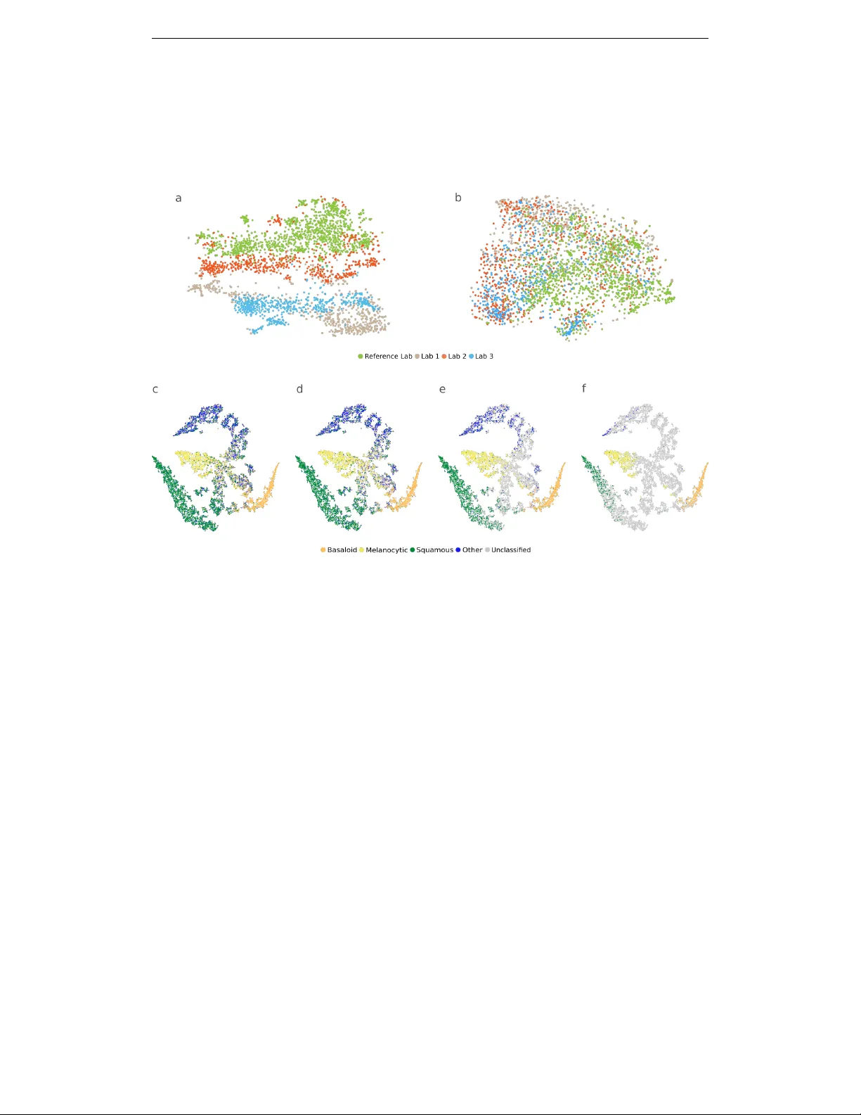
A ugmenting the P athology Lab: An Intelligent Whole Slide Image Classification System f or the Real W orld Julianna D. Ianni ∗ , 1 , Rajath E. Soans ∗ , 1 , Siv aramakrishnan Sankarapandian 1 , Ramachandra V ikas Chamarthi 1 , Devi A yyagari 1 , Thomas G. Olsen 2 , 3 , Michael J. Bonham 1 , Coleman C. Stavish 1 , Kiran Motaparthi 4 , Clay J. Cockerell 5 , Theresa A. Feeser 1 , Jason B. Lee 6 ∗ These authors contributed equally to this w ork. 1 Proscia Inc., Philadelphia, Pennsylvania, USA. 2 Department of Dermatology , Boonshoft School of Medicine, Wright State Univ ersity School of Medicine, Dayton, Ohio, USA 3 Dermatopathology Laboratory of Central States, Dayton, Ohio, USA 4 Department of Dermatology , Univ ersity of Florida College of Medicine, Gainesville, Florida 5 Cockerell Dermatopathology , Dallas, T exas, USA. 6 Departments of Dermatology and Cutaneous Biology , Sidney Kimmel Medical College at Thomas Jefferson Univ ersity , Philadelphia, Pennsylvania, USA. A B S T R AC T Standard of care diagnostic procedure for suspected skin cancer is microscopic examination of hematoxylin & eosin stained tissue by a pathologist. Areas of high inter-pathologist discordance and rising biopsy rates necessitate higher efficiency and diagnostic reproducibility . W e present and validate a deep learning system which classifies digitized dermatopathology slides into 4 categories. The system is dev eloped using 5,070 images from a single lab, and tested on an uncurated set of 13,537 images from 3 test labs, using whole slide scanners manufactured by 3 different vendors. The system’ s use of deep-learning-based confidence scoring as a criterion to consider the result as accurate yields an accuracy of up to 98%, and makes it adoptable in a real-world setting. W ithout confidence scoring, the system achiev ed an accuracy of 78%. W e anticipate that our deep learning system will serv e as a foundation enabling faster diagnosis of skin cancer , identification of cases for specialist revie w , and targeted diagnostic classifications. 1 1 I N T RO D U C T I O N Every year in the United States, 12 million skin lesions are biopsied, 1 with over 5 million new skin cancer cases diagnosed. 2 After a skin lesion is biopsied, the tissue is fixed, embedded, sectioned, and stained with hematoxylin and eosin (H&E) on glass slides, ultimately to be examined under microscope by a dermatologist, general pathologist or dermatopathologist who pro vides a diagnosis for each tissue specimen. Owing to the large variety of over 500 distinct skin pathologies 3 and the sev ere consequences of a critical misdiagnosis, 4 diagnosis in dermatopathology demands special- ized training and education. Although the inter-observ er concordance rate in dermatopathology is estimated to be between 90 and 95%, 5, 6 there are some distinctions which present frequent disagree- ment among pathologists, such as in the case of melanoma vs. melanocytic nevi. 7–11 Any system which could improve diagnostic accuracy provides obvious benefits for dermatopathology labs and patients; howe ver , there are substantial benefits also to improving the distribution of pathologists’ workloads. 12–14 This can reduce diagnostic turnaround times in sev eral scenarios. For example, when skin biopsies are interpreted initially by a dermatologist or a general pathologist, prior to re- ferral to a dermatopathologist, it can result in a delay of days, sometimes in critical cases. In another common scenario, additional staining is required to identify characteristics of the tissue not cap- tured by standard H&E staining. If those additional stains are not ordered early enough, there can be further delays to diagnosis. An intelligent system to distribute pathology workloads could alleviate some of these bottlenecks in lab workflows. The rise in adoption of digital pathology 1, 15 provides an opportunity for the use of deep learning-based methods for closing these gaps in diagnostic reli- ability and efficienc y . 16, 17 In recent years, deep neural networks have proven capable of identifying diagnostically relev ant patterns in radiology and pathology . 18–25 While deep learning applied to medical imaging-based diagnostic applications has progressed beyond proof-of-concept, 18, 20, 22–24 the translation of these methods to digital pathology must ov ercome unique challenges. Among these is sheer image size; a whole slide image (WSI) can contain sev eral gigabytes of data and billions of pixels. Additionally , non-standardized image appearance (variability in tissue preparation, staining, scanned appearance, presence of artifacts) and a large number of pathologic abnormalities that can be observed present unique barriers to de velopment of deployable deep learning applications in pathology . For example, 2 T ellez et al. 26 demonstrate the strong impact that inter-site variance– with respect to stain and other image properties– can have on deep learning models. Nonetheless, deep learning-based methods hav e recently sho wn promise in a number of tasks in digital pathology , primarily for segmentation models and networks which classify small patches within a WSI. 19, 26–35 More recent methods hav e performed direct WSI classification. 21, 25, 36 Howe ver , man y focus only on a single diagnostic class to make binary classifications, 19, 25, 31, 36 the utility of which breaks down in addressing subspecialties for which there is more than one relev ant pathology of interest. Additionally , man y of these methods hav e focused on curated datasets consisting of fewer than 5 pathologies with little diagnostic and image variability . 19, 21, 31, 36 The insufficienc y of models dev eloped and tested using small curated datasets such as CAMEL Y ON 29 was effecti vely demonstrated by Campanella et. al. 25 Howe ver , while this study claimed to validate on data free of curation, the data presented featured limited capture of not only biological v ariability (e.g. exclusion of commonly-occurring prostatic interaepithelial neoplasia and atypical glandular morphologies) but also image variability originating from slide preparation and scanning characteristics (e.g. exclusion of slides with pen markings, need for retrospectiv e human correction of select results, and poorer performance on externally-scanned images). In contrast to deep learning systems exposed to contri ved pathology problems and datasets, pathologists are trained to recognize hundreds of morphological variants of diseases they are likely to encounter in their careers and must adapt to variations in tissue preparation and staining protocols. In addition to these variations, deep learning algorithms can also be sensitiv e to image artifacts. Some research has attempted to account for these issues by detecting and pre-screening image artifacts, either by automatically 37–39 or manually removing slides with artifacts. 19, 25, 31 Campanella et. al 25 include variability in allowed artifacts which others lack, b ut still selecti vely e xclude images with ink mark- ings, which hav e been shown to af fect predictions of neural networks. 40 A real-world deep learning pathology system must be demonstrably robust to these variations. It must be tested on non-selected specimens, with no exclusions and no manual pre-screening of slides input or post-screening of the system outputs. A comprehensiv e test set for robustly assessing system performance should contain images: 3 1. From multiple labs, with mark edly v aried stain and image appearance due to imaging using different whole slide image scanner models and vendors, and variability in tissue prepara- tion and staining protocols. 2. Wholly representati ve of a diagnostic workload in the subspecialty (i.e. not excluding pathologic or morphologic variations which occur in a sampled time-period). 3. W ith a host of naturally-occurring and human-induced artifacts: scratches, tissue fixation artifacts, air bubbles, dust and dirt, smudges, out-of-focus or blurred regions, scanner- induced misregistrations, striping, pen ink or letters on slides, inked tissue margins, patch- ing errors, noise, color/calibration/light variations, knife-edge artifacts, tissue folds, and lack of tissue present. 4. W ith no visible pathology (in some instances), or with no conclusiv e diagnosis, cov ering the breadth of cases occurring in diagnostic practice. In this work, we present a pathology deep learning system (PDLS) which is capable of classifying WSIs containing H&E-stained skin biopsies or excisions into diagnostically-relev ant classes (Basa- loid, Squamous, Melanocytic and Other). A key aspect of our system is that it returns a measure of confidence in its assessment; this is necessary in such classifications because of the wide range of variability in the images. A real-world system should not only return accurate predictions for commonly occurring diagnostic entities and image appearances, but also flag the non-negligible re- mainder of images whose unusual features lie outside the range allowing reliable model prediction. The PDLS is developed using 5,070 WSIs from a single lab ( ”Reference Lab” ), and independently tested on a completely uncurated and unrefined set of 13,537 sequentially accessioned H&E-stained images from 3 additional labs, each using a different scanner and different staining and preparation protocol. No images were excluded. T o our knowledge, this test set is the largest in pathology to date. Our PDLS satisfies all the criteria listed abov e for real-world assessment, and is therefore to our knowledge the first truly real-w orld-validated deep learning system in pathology . 4 2 R E S U L T S 2 . 1 O V E R V I E W A N D E V A L UA T I O N O F P D L S The proposed system, as illustrated in Fig. 1, takes as input a WSI and classifies it using a cascade of three independently-trained conv olutional neural netw orks (CNNs) as follows: The first ( CNN-1 ) adapts the image appearance to a common feature domain, accounting for variations in stain and appearance; the second ( CNN-2 ) identifies regions of interest (ROI) for processing by the final net- work ( CNN-3 ), which classifies the WSI into one of 4 classes defined broadly by their histologic characteristics—Basaloid, Melanocytic, Squamous, and Other , as further described in Methods. Al- though the classifier operates at the level of an individual WSI, some specimens are represented by multiple WSIs, and therefore these predictions are aggregated to produce a single specimen-level classification. The classifier is trained such that for each image a predicted class is returned along with a confidence in the accuracy of the outcome. This allows discarding of predictions that are determined by the PDLS as likely to be false. Since there is a large amount of variation in both pathologic findings of skin lesions as well as scan- ner or preparation-induced abnormalities, it is very important for the model to assess a confidence score for each decision; thereby , likely-misclassified images can be flagged as such. W e dev eloped a method of confidence scoring based on Gal et al. 41 and set confidence thresholds a priori based only on performance on the validation set of the Reference Lab, which is independent of the data for which we report all measures of system performance (see Methods). Three confidence thresholds were calculated and fixed based on the Reference Lab v alidation set such that discarding specimens with lo wer scores achieved the following 3 le vels of accuracy in the remainder: 90% (Le vel 1), 95% (Lev el 2) and 98% (Lev el 3). T o achieve high classification accuracy in the presence of a wide range of variability in tissue ap- pearance between labs, a unique calibration set (about 520 WSIs) was collected from each lab and used to fine-tune the final classifier (CNN-3). Results are reported only on the test set, consisting of 13,537 WSIs from the 3 test labs which were not used in model training or dev elopment. The deep learning s ystem ef fectiv ely classifies WSIs into the 4 classes with an ov erall accurac y of 78% before thresholding on confidence score. Importantly , in specimens whose predictions exceeded the confi- 5 Figure 1: The process of classifying a whole slide image (WSI) with the pathology deep learning system is shown. The input WSI is first segmented and divided into tissue patches (Tissue Seg- mentation, T iling); those patches pass through CNN-1, which adapts their stain and appearance to the target domain; they then pass through CNN-2 which identifies the regions of interest (patches) required to pass to CNN-3, which performs a 4-way classification, and repeats this 30 times to yield 30 predictions, where each prediction P i is a vector of dimension N classes =4; the max of the class- wise mean of sigmoid output is the confidence score. If the confidence score surpasses a pre-defined threshold, the corresponding class decision is assigned. 6 dence threshold, the PDLS achiev ed an accuracy of 83%, 94%, and 98% for confidence le vels 1, 2 and 3, respecti vely . Performance of the PDLS is characterized with receiver operating characteristic (R OC) curves, shown for each of the 4 classes in Fig. 2a-d at each confidence lev el; as confidence lev el increases, a larger percentage of images do not meet the threshold and are excluded from the analysis, as indicated by the colorbar . At Lev els 1, 2, and 3, the percentage of test specimens ex- ceeding the confidence threshold was 83%, 46% and 20%, respectively . Area under the curve (A UC) increased with increasing confidence level. Similar results are sho wn for Lev el 1 for each test lab in Fig. 2f-i which compare A UC and percentage of specimens confidently classified between the 3 labs. Fig. 3 sho ws the mapping of ground truth class to the proportion correctly predicted as well as proportions confused for each of the other classes or remaining unclassified (at Level 1) due to lack of a confident prediction or absence of any ROI detected by CNN-2. Additionally , this figure sho ws the most common ground-truth diagnoses in each of the 4 classes found in the test set. 2 . 2 R E D U C T I O N O F I N T E R - S I T E V A R I A N C E T o demonstrate that the image adaptation performed by CNN-1 effecti vely reduces inter-site varia- tions, we used t-distrib uted stochastic neighbour embedding (t-SNE) to compare the feature space of CNN-2 with and without first performing the image adaptation step. W e show CNN-2’ s embedded feature space without first performing image adaptation in Fig. 4a; Fig. 4b then shows the embedded feature space from CNN-2 when image adaptation is performed first. Inclusion of the image adapta- tion step results in more ov erlapped distrib utions in feature space than those produced without using image adaptation; this transformation into a common feature space allows the system to perform high-quality classification regardless of staining technique or scanner used. 2 . 3 E FF E C T I V E C L A S S S E PA R A T I O N Additionally , we used t-SNE to show class separation based on the internal feature representation learned by the final classifier (CNN-3), as shown in Fig. 4c. Each point in these t-SNE plots rep- resents a single specimen with color denoting its ground-truth class. Figs. 4d-f show the same information when thresholding at each of the 3 confidence levels (1-3, respectiv ely), indicating in 7 Figure 2: Receiv er operating characteristic (ROC) curves are shown by lab, class, and confidence lev el for the test set of 13,537 images. R OC curves are shown for Basaloid (a,g), Melanocytic (b,h), Squamous (c,i) and Other (d,f) classes, with percentage of specimens classified for each curve represented by the color bar at right. The three curves in each of (a-d) represent the respectiv e thresholded confidence le vels or no confidence threshold (”None”). The three curv es in each of (f-i) represent the three labs. (e) V alidation set accuracy in the Reference Lab is plotted versus sigmoid confidence score, with dashed lines corresponding to the sigmoid confidence thresholds set (and fixed) at 90% (Le vel 1), 95% (Le vel 2), and 98% (Le vel 3). 8 Figure 3: Sankey diagram depicting the mapping of ground truth classes to the top 5 most common diagnostic entities in the test set in each class (left). Malignant melanoma was not in the top 5 but included here due to its clinical importance. Also shown is the proportion of images correctly classified, along with the distrib ution of misclassifications and unclassified specimens (those for which confidence score was below the threshold) at confidence Lev el 1 (right). The width of each bar is proportional to the corresponding number of specimens found in the 3-lab test set. gray the specimens left unclassified at each. The clustering shows strong class separation between the 4 classes, with stronger separation and fewer specimens classified as confidence le vel increases. 2 . 4 T I M I N G P R O FI L E It is important that ex ecution time for any system intended to be implemented in a lab workflo w be low enough to not present a bottleneck to diagnosis. Therefore, the proposed system was designed to be parallelizable across WSIs to enhance throughput and meet the ef ficiency demands of the real- world system. On a single compute node (described in Methods), the median processing time per WSI was 137 seconds, with overall throughput of 40 WSIs/hour . Fig. 5a shows the median time consumed by each stage in the pipeline, and Fig. 5b shows box-plots of time at each stage, as well as end-to-end ex ecution time. 9 Figure 4: Image feature vectors are shown in 2-dimensional t-distributed stochastic neighbor em- bedded (t-SNE) plots. T op: Feature embeddings from CNN-2 are sho wn with a) no prior image adaptation and b) when image adaptation (using CNN-1) is performed prior to performing region of interest (ROI) e xtraction using CNN-2. Each point is an image patch within a whole slide image (WSI), colored by lab. Bottom: Feature embeddings from CNN-3, where each point represents a specimen and is colored according to ground-truth classification. All specimens are classified at baseline (a), where (d-f) show increasing confidence thresholds (d=Level 1, e=Level 2, f=Level 3), with specimens not meeting the threshold in gray . 10 Figure 5: PDLS compute time for whole slide images on the calibration sets from the 3 test labs. (a) The median percentage of total computation time for each stage in PDLS is shown. (b) A boxplot of the computation time in seconds required at each stage of the pipeline is shown on a logarithmic scale, along with total end-to-end ex ecution time for all images (dark brown, median 137s), and excluding images for which no re gions of interest are detected (light brown, median 142s). 11 3 D I S C U S S I O N Our work demonstrates the ability of a multi-site generalizable PDLS to accurately classify the majority of specimens in a routine dermatopathology lab workflo w . Dev eloping a deep-learning-based classification which translates across image sets from multiple labs is non-tri vial. 25, 26, 30 W ithout compensation for image variations, non-morphological differ - ences between data from different labs are more prominent in the feature space than morphological differences between the specimens ultimately belonging to the same diagnostic classification. This is demonstrated in Fig. 4a, in which the image patches cluster according to the lab that prepared and scanned the corresponding slide. When image adaptation is performed prior to computing image features, the images do not strongly cluster by lab (Fig. 4b). In this study , we demonstrate that a PDLS trained on a single Reference Lab can be effecti vely calibrated to 3 additional lab sites. Figs. 4c-f show strong class separation between 4 classes, and this class separation strengthens with in- creasing confidence threshold. Intuitively , low-confidence images cluster at the intersection of the 4 classes. Strong class separation is reflected also in the R OC curves, which show high A UC across classes and labs, as seen in Fig. 2. A UC increases with increased confidence lev el, demonstrating the utility of confidence score thresholding as a tunable method for excluding poor model predic- tions. Figs. 2d shows relativ ely worse performance in the Other class. In 4c it can be seen that there is some overlap between the Squamous and Other classes in feature space; Fig. 3 also shows some confusion between these two classes, but overall, demonstrates accurate classification of the majority of specimens from each class. The majority of previous deep learning systems in digital pathology have been validated only on a single lab or scanner’ s images, 19, 21, 25 curated datasets that ignored a portion of lab volume within a speciality , 19, 25, 32 and tested on small and unrepresentative datasets, 19, 21, 32, 35 excluded images with artifacts 19, 25, 31 or selectiv ely rev erse image ”ground truth” retrospectively for misclassifications 25 and train patch- or se gmentation-based models while using traditional computer vision or heuristics to arri ve at a whole slide prediction. 19, 29, 31 These methods do not lend themselves to real-world enabled deep learning systems that are capable of operating independent of the pathologist and prior to pathologist revie w . These systems would require some human intervention before they can 12 provide useful information about a slide, and therefore do not enable improv ements in lab workflow efficiencies. In contrast, our PDLS is trained on all av ailable slides– images with artifacts, slides without tissue on them, slides with poor staining or tissue preparation, slides exhibiting rare pathology , and those with very subtle e vidence of pathology . All of this v ariability in the data necessitates that our PDLS is capable of determining when it is not likely to make a well-informed prediction. This is accom- plished with a confidence score, which can be thresholded to obtain better system performance as shown in Fig. 2a-e. Correlation between system accuracy and confidence was established a priori using only the Reference Lab validation set (Fig. 2e) to fix the 3 confidence thresholds. By fixing thresholds a priori we establish that they are generalizable. Campanella et al. 25 hav e attempted to similarly set a classification threshold which yields optimal performance; howe ver , they perform this thresholding using the last layer output of a model, on the same test set in which they report it yielding 100% sensitivity; therefore they do not demonstrate the generalizability of this tuned pa- rameter . Secondly , as Gal et. al 41 demonstrate, a model’ s predictive probability (last layer output) cannot be interpreted as a measure of confidence. W e report all performance measures (accuracy , A UC) at the level of a specimen, which may consist of several slides, since diagnosis is not reported at the slide lev el in dermatopathology . W e aggre gate all slide-le vel decisions to the specimen level as reported in Methods; this is particularly important as not all slides within a specimen will exhibit pathology , and therefore an incorrect prediction can be made if slide-lev el-reporting is performed. Similar systems 19, 25, 35, 36 hav e not attempted to solve the problem of aggregating slide-decisions to the specimen le vel at which diagnosis is performed. For the PDLS to operate before pathologist assessment, the entire pipeline must be able to run in a time period that av oids delaying the presentation of a case to the pathologist. The compute time profile shown in Fig. 5a-b demonstrates that the PDLS can classify a WSI in under 3 minutes in the majority of cases, which is on the same order of the amount of time it takes for today’ s scanners to scan a single slide. There was considerable variation in this number due to a large amount of variability in the size of the tissue. Howe ver , it is important to note that this process can be infinitely parallelized across WSIs to enhance throughput. Additional optimization of this process is possible and is the subject of future work. There are several limitations to the current 13 PDLS which are shared by pre vious implementations of deep learning image classification in digital pathology . First, when diagnosing a specimen, pathologists often have access to additional clinical information about the case, whereas our PDLS uses only WSIs to make a prediction. T raining the PDLS with this additional clinical conte xt as input would lik ely improve accuracy in some cases. A second limitation is that all existing systems for pathology classification attempt to put restrictions on the biology , namely that a WSI or a specimen can only represent a single diagnosis. Rarely (2-3% of specimens), a specimen should be labelled with more than one class. W e did not train the current PDLS to handle this special case since the av ailable sample of images with dual ground-truth class is small; howe ver , this will be a subject of future research. While the current PDLS does not make diagnostic predictions, its classification has the potential to increase diagnostic efficienc y and consistency in se veral scenarios. For example, pathologists might choose to prioritize certain classes, e.g. Melanocytic, that may contain more difficult cases, requiring longer re view time, additional lev els ordered, or ancillary testing such as immunostains. Similarly , a dermatologist who interprets biopsies could choose to only receiv e cases classified as Basaloid, and a void recei ving many inflammatory cases or melanocytic lesions which might be sent for referral. The tunability of the confidence threshold in the model as a near-final step in assigning a classification has further implications for how this deep learning system might be utilized in practice. For applications that depend on high-sensitivity classification (e.g. treating classification as a form of quality assurance to assist in av oiding missed diagnosis of melanomas, which should exist in the Melanocytic classification), a higher confidence threshold might be set. Similarly , for an application that depends less on specificity (e.g. triage of cases to balance pathologists’ workloads) the desired confidence threshold could be lower , thereby av oiding an ov erly-large set of unclassified specimens. Finally , as hierarchical classification models have been shown to outperform flat classifiers, 42 we expect that the current PDLS serves as a basis for extension to diagnostic classification systems. This would enable further prioritization of more critical cases, such as those presenting features of melanoma. 14 3 . 1 C O N C L U S I O N The techniques presented herein–namely deep learning of heterogeneously-composed classes, and confidence-based prediction screening– are not limited to application in dermatopathology or ev en pathology , but broadly demonstrate potentially ef fectiv e strategies for translational application of deep learning in medical imaging. The PDLS presented deliv ers accurate prediction, regardless of scanner type or lab, and requires minimal calibration to achiev e accurate results for a new lab . The system is capable of assessing which of its decisions are viable based on a computed confidence score, and thereby can filter out predictions that are unlikely to be correct. This confidence-based strategy is broadly applicable for achieving the low error rates necessary for the practical use of machine learning in challenging and nuanced domains of medical disciplines. 4 M E T H O D S 4 . 1 D A TA U S E D I N D E V E L O P M E N T The proposed system was developed in its entirety using H&E-stained WSIs from Dermatopathol- ogy Laboratory of Central States, which is referred to as the Reference Lab in this work. All slides from this Reference Lab were scanned using the Leica Aperio A T2 Scanscope (Aperio, Le- ica Biosystems, V ista, California). This dataset is made up of two subsets, the first (3,070 WSIs) consisting of images representing commonly diagnosed dermatopathologic entities, and the second (2,000 slides) consisting of all cases accessioned during a discrete period of time, representing the typical distribution seen by the lab . This combined Reference Lab set of 5,070 WSIs was partitioned randomly into training (70%), validation (15%), and testing (15%) sets, such that WSIs from any giv en specimen were not split between sets. 4 . 2 T A X O N O M Y The design of target classes in this study is heavily influenced by the preva lence of each class’ s constituent pathologies and the presence of visually- and histologically-similar class-representative features. They capture, in roughly equal proportion, the majority of diagnostic entities seen in a dermatopathology lab practice. Specifically , we perform classification of WSIs into four classes: 15 Basaloid, Squamous, Melanocytic, and Others. These four classes are defined by the following histological descriptions of their features: 1. Basaloid : Abnormal proliferations of basaloid-ov al cells having scant cytoplasm and fo- cal hyperchromasia of nuclei; cells in islands of variable size with round, broad-based and angular morphologies; peripheral palisading of nuclei, peritumoral clefting, and a fi- bromyxoid stroma. 2. Squamous : Squamoid epithelial proliferations ranging from a hyperplastic, papillomatous and thickened spinous layer to focal and full thickness atypia of the spinous zone as well as in vasi ve strands of atypical epithelium e xtending into the dermis at various le vels. 3. Melanocytic : Cells of melanocytic origin in the dermis, in symmetric, nested, and dif- fuse aggregates and within the intraepidermal compartment as single cell melanocytes and nests of melanocytes. Nests may be variable in size, irregularly spaced, and single cell melanocytes may be solitary , confluent, hyperchromatic, pagetoid and with pagetoid spread into the epidermis. Cellular atypia can range from none to striking anaplasia and may be in situ or in vasi ve. 4. Other : Morphologic and histologic patterns that include either the absence of a specific abnormality or one of a wide v ariety of other neoplastic and inflammatory disorders which are both epithelial and dermal in location and etiology , and which are confidently classified as not belonging to Classes 1-3. These four classes account for more than 200 diagnostic entities in our test set, and their mapping to the most prev alent diagnostic entities in the test set is illustrated in Fig. 3. 4 . 3 S Y S T E M D E S I G N A N D T R A I N I N G Our image processing pipeline for the PDLS is illustrated in Fig. 1. The PDLS takes as input a WSI, segments out re gions containing tissue, and divides these regions into a set of tiles, each of size 128 × 128 pixels. The process of assigning a label to a WSI using this set of tiles is comprised of three stages: 1) Image Adaptation, 2) Region of Interest Extraction, and 3) WSI Classification. 16 Since the PDLS is trained on only a single lab’ s data, it is critical to perform image adaptation to adapt images received from test labs to a domain in which the image features are interpretable by the PDLS. W ithout adaptation, unaccounted-for variations in the images due to staining and scanning protocols can critically af fect the performance of CNNs. 25, 26, 30 The PDLS performs image adaptation using a CNN (referred to as CNN-1), which takes as input an image tile and outputs an adapted tile of the same size and shape but with standardized image appearance. CNN-1 was trained using 300,000 tiles from the Reference Lab and mimics the av erage image appearance from the Reference Lab giv en an input tile. Subsequently , R OI extraction is performed using a second CNN (referred to as CNN-2). This CNN is trained using expert annotations by a dermatopathologist as the ground truth. It performs a seg- mentation of regions e xhibiting abnormal features indicative of pathology . The model takes input of a single tile and outputs a se gmentation map. T iles are selected corresponding to the positiv e regions of the segmentation map; the set of all identified tiles of interest, t from a WSI is passed on to the final stage classifier . The final WSI classification is then performed using a third CNN (CNN-3), which predicts a label, l for the set of tiles t identified by CNN-2 where: l ∈ { Basaloid , Squamous , Melano cytic , Others } . (1) CNN-3 additionally outputs a confidence score for each WSI. In clinical practice, and in our dataset, diagnostic labels are reported at the le vel of a specimen, which may be represented by one or se veral WSIs. Therefore, the predictions of the PDLS are aggregated across WSIs to the specimen lev el; this is accomplished by assigning to a gi ven specimen the maximum-confidence prediction across all WSIs representing that specimen. 4 . 4 C A L I B R AT I O N A N D V A L I D A T I O N F O R A D D I T I O N A L S I T E S T o demonstrate its robustness to v ariations in scanners, staining, and image acquisition protocols, the PDLS was tested on 13,537 WSIs collected from 3 dermatopathology labs, representing tw o leading dermatopathology labs in top academic medical centers (Dermatopathology Center at Thomas Jef- ferson Univ ersity and the Department of Dermatology at Uni versity of Florida College of Medicine) and a high volume national priv ate dermatopathology laboratory (Cock erell Dermatopathology).W e 17 refer to these as test labs . Prior to the study , each lab sought study approval from the appropri- ate Institutional Re view Board and was exempted. Each lab performed scanner v alidation prior to data collection, according to the guidelines of the College of American Pathologists. 43 Each test lab selected a date range within the past 4 years (based on slide av ailability) from which to scan a sequentially accessioned set of approximately 5,000 slides. Each of the 3 test labs scanned their slides using a different scanner vendor and model. Scanner models used were: Leica Ape- rio A T2 Scanscope Console (Leica Biosystems, V ista, California), Hamamatsu Nanozoomer-XR (Hamamatsu Photonics, Hamamatsu City , Shizuoka, Japan), and 3DHistech Pannoramic 250 Flash III (3DHistech, Budapest, Hungary). All parameters and stages of the PDLS pipeline were held fixed after de velopment on the Reference Lab, with the exception of CNN-3, whose weights were fine-tuned independently for each lab using a calibration set of approximately 520 WSIs. (W e re- fer to this process as calibration). The calibration set for each lab consisted of approximately 500 sequentially-accessioned WSIs (pre-dating the test set) supplemented by 20 additional WSIs from melanoma specimens. Of these calibration images, 80% were used for fine-tuning, and 20% for lab- specific validation of the fine-tuning and image adaptation procedures. Specimens from the same patient were not split between fine-tuning, v alidation and test sets. After this calibration, all pa- rameters were permanently held fixed, and the system was run only once on each lab’ s test set of approximately 4,500 WSIs (range 4451 to 4585)– 13,537 in total. 4 . 5 C O N FI D E N C E S C O R I N G A N D T H R E S H O L D C O M P U TA T I O N Gal et al. 41 propose a method to reliably measure the uncertainty of a decision made by a classifier . W e hav e adapted this method for confidence scoring of the decision made by PDLS. T o determine a confidence score for a WSI we perfom prediction on the same WSI repeatedly for (using CNN-3) sev eral times by omitting a random subset of neurons (here 70%) in CNN-3 from the prediction. Each repetition results in a prediction made using a dif ferent subset of feature representations. Here, we use T = 30 repetitions, where each repetition i yields a prediction P i , a vector of sigmoid v alues of length equal to the number of classes. Each element of P i represents the binary probability , p i,c , of the corresponding WSI belonging to class c . The confidence score s for a giv en WSI is then 18 computed as follows: s = max c P T i =1 p i,c T ! (2) The class associated with the highest confidence s is the predicted class for the WSI. Finally , the specimen prediction is assigned as the maximum-confidence prediction of its constituent WSI pre- dictions. If a specimen’ s confidence score is below a certain threshold, then the prediction is con- sidered unreliable and the specimen remains unclassified. Three threshold v alues for the confidence score were selected for analysis; these were determined during the de velopment phase, using only the Reference lab’ s data, because this confidence threshold is a parameter which can tune model performance. Confidence thresholds were selected such that discarding specimens with sigmoid confidence lower than the threshold yielded a pre-defined level of accuracy in the remaining spec- imens of the validation set of the Reference Lab . The three target accuracy lev els were 90%, 95% and 98%; the corresponding sigmoid confidence thresholds of 0.33, 0.76, and 0.99 correspond to confidence Le vels 1, 2, and 3 respecti vely; these confidence thresholds were held fixed, and applied without modification to the test sets from the 3 test labs. 4 . 6 C O M P U T E T I M E Compute time profiling of the PDLS was performed on an Amazon W eb Services EC2 P3.8x large instance equipped with 32 core Intel Xeon E5-2686 processors, 244 GB RAM, and four 16GB NVIDIA T esla v100 GPUs supported by NVLink for peer-to-peer GPU communication. Compute time was measured on the calibration sets of each of the the test labs. Acknowledgements W e would like to thank Hamamatsu and Epredia for loaning whole slide image scanners. W e thank Katherine T esno, Denise Lunsford, Cindy Jones, Cassandra Mor gan, V alerie Matteo, Doa Salabi, and Craig Reed all for their hard work in scanner operation and data collection, and Mary Bohannon for study coor- dination, IRB support and scanner operation. W e are grateful also to Michael Kent, Ph.D. for scientific advice and discussion, Nathan Buchbinder for help with study coordination and manuscript revie w , Saul Kohn, Ph.D. for manuscript revie w , and Addie W alker , M.D. and Vladimir V incek, M.D., Ph.D. for revie w of specimens. R E F E R E N C E S 1. Klipp, J. The U .S. Anatomic P athology Market: F or ecast & T r ends 2017-2020 . Laboratory Economics. 19 2. Rogers, H. W ., W einstock, M. A., Feldman, S. R. & Coldiron, B. M. Incidence estimate of non- melanoma skin cancer (keratinoc yte carcinomas) in the US population, 2012. J AMA Dermatol 151 , 1081–1086 (2015). 3. Feramisco, J. D., Sadreyev , R. I., Murray , M. L., Grishin, N. V . & Tsao, H. Phenotypic and genotypic analyses of genetic skin disease through the online mendelian inheritance in man (omim) database. J Investig Dermatol 129 , 2628–2636 (2009). 4. Olhof fer, I. H., Lazov a, R. & Leffell, D. J. Histopathologic misdiagnoses and their clinical consequences. Ar ch Dermatol 138 , 1381–1383 (2002). 5. K ent, M. N. et al. Diagnostic accuracy of virtual pathology vs traditional microscopy in a large dermatopathology study . J AMA Dermatol 153 , 1285–1291 (2017). 6. Shah, K. K. et al. V alidation of diagnostic accuracy with whole-slide imaging compared with glass slide revie w in dermatopathology . J Am Acad of Dermatol 75 , 1229–1237 (2016). 7. Farmer , E. R., Gonin, R. & Hanna, M. P . Discordance in the histopathologic diagnosis of melanoma and melanocytic ne vi between expert pathologists. Hum P athol 27 , 528–531 (1996). 8. Corona, R. et al. Interobserver variability on the histopathologic diagnosis of cutaneous melanoma and other pigmented skin lesions. J Clin Oncol 14 , 1218–1223 (1996). 9. Lodha, S., Saggar, S., Celebi, J. T . & Silvers, D. N. Discordance in the histopathologic diagnosis of difficult melanoc ytic neoplasms in the clinical setting. J Cutan P athol 35 , 349–352 (2008). 10. Elmore, J. G. et al. Pathologists’ diagnosis of inv asive melanoma and melanocytic prolifera- tions: observer accurac y and reproducibility study . BMJ 357 , j2813 (2017). 11. Shoo, B. A., Sagebiel, R. W . & Kashani-Sabet, M. Discordance in the histopathologic diagnosis of melanoma at a melanoma referral center . J Am Acad Dermatol 62 , 751 – 756 (2010). 12. Baidoshvili, A. et al. Evaluating the benefits of digital pathology implementation: time sa vings in laboratory logistics. Histopathology 73 , 784–794 (2018). 13. Ho, J. et al. Can digital pathology result in cost savings? a financial projection for digital pathology implementation at a large integrated health care organization. J P ath Inform 5 , 33 (2014). 20 14. Hanna, M. G. et al. Whole slide imaging equiv alency and efficiency study: experience at a lar ge academic center . Mod P athol 32 , 916–928 (2019). 15. Al-Janabi, S., Huisman, A. & V an Diest, P . J. Digital pathology: current status and future perspectiv es. Histopathology 61 , 1–9 (2012). 16. Cruz-Roa, A. et al. Accurate and reproducible inv asiv e breast cancer detection in whole-slide images: A deep learning approach for quantifying tumor extent. Sci Rep 7 , 46450 (2017). 17. Litjens, G. et al. Deep learning as a tool for increased accuracy and efficiency of histopatho- logical diagnosis. Sci Rep 6 , 26286 (2016). 18. Ardila, D. et al. End-to-end lung cancer screening with three-dimensional deep learning on low-dose chest computed tomograph y . Nat Med 25 , 954–961 (2019). 19. Olsen, T . G. et al. Diagnostic performance of deep learning algorithms applied to three common diagnoses in dermatopathology . J P athol Inform 9 , 32 (2018). 20. Este va, A. et al. Dermatologist-level classification of skin cancer with deep neural networks. Natur e 542 , 115–118 (2017). 21. Li, J. et al. An attention-based multi-resolution model for prostate whole slide image classifi- cation and localization. Preprint at: https://arxiv .org/abs/1905.13208 . 22. Abr ` amoff, M. D. Pi votal trial of an autonomous AI-based diagnostic system for detection of diabetic retinopathy in primary care of fices. NPJ Digit Med 1 , 39 (2018). 23. Y ao, L. et al. Learning to diagnose from scratch by exploiting dependencies among labels. Preprint at https://arxiv .org/abs/1710.10501 (2017). 24. Hwang, E. J. et al. Development and validation of a deep learning-based automated detection algorithm for major thoracic diseases on chest radiographs. J AMA Network Open 2 (2019). 25. Campanella, G. et al. Clinical-grade computational pathology using weakly supervised deep learning on whole slide images. Nat Med 25 , 1301–1309 (2019). 26. T ellez, D. et al. Quantifying the effects of data augmentation and stain color nor- malization in conv olutional neural networks for computational pathology . Preprint at: https://arxiv .org/abs/1902.06543 (2019). 21 27. K orbar , B. et al. Deep learning for classification of colorectal polyps on whole-slide images. J P ath Inform 8 , 1–12 (2017). 28. Sornapudi, S. et al. Deep learning nuclei detection in digitized histology images by superpixels. J P ath Inform 9 , 5 (2018). 29. A wan, R., K oohbanani, N. A., Shaban, M. & Rajpoot, N. Context-a ware learning us- ing transferable features for classification of breast cancer histology images. Preprint at https://arxiv .org/abs/1803.00386 (2018). 30. Ciompi, F . et al. The importance of stain normalization in colorectal tissue classification with con volutional netw orks. Pr oc IEEE Int Sym Biomed Imaging 160–163 (2019). 31. Bulten, W . et al. Automated gleason grading of prostate biopsies using deep learning. Preprint at: https://arxiv .org/abs/1907.07980 . 32. Ghaznavi, F ., Ev ans, A., Madabhushi, A. & Feldman, M. Digital imaging in pathology: Whole- slide imaging and beyond. Annu Rev P athol-Mech 8 , 331–359 (2013). 33. Bejnordi, B. E. et al. Using deep con volutional neural networks to identify and classify tumor- associated stroma in diagnostic breast biopsies. Mod P athol 31 , 1502–1512 (2018). 34. Jano wczyk, A. & Madabhushi, A. Deep learning for digital pathology image analysis: A com- prehensiv e tutorial with selected use cases. J P ath Inform 7 , 29 (2016). 35. Hart, S. N., Flotte, W . & Andrew , P . Classification of melanoc ytic lesions in selected and whole slide images via con volutional neural netw orks. J P athol Inform 10 , 5 (2019). 36. Ing, N. et al. A deep multiple instance model to predict prostate cancer metastasis from nuclear morphology . In Pr oc Int Conf Med Imag Deep Learning (2018). 37. K ohlberger , T . et al. Whole-slide image focus quality: Automatic assessment and impact on AI cancer detection. Preprint at: https://arxiv .org/abs/1901.04619 (2019). 38. Senaras, C., Niazi, M. K. K., Lozanski, G. & Gurcan, M. N. DeepF ocus: detection of out-of- focus regions in whole slide digital images using deep learning. PLoS ONE 13 (2018). 39. Jano wczyk, A., Zuo, R., Gilmore, H., Feldman, M. & Madabhushi, A. HistoQC: an open-source quality control tool for digital pathology slides. JCO Clin Cancer Inform 1–7 (2019). 22 40. Ali, S. & May , C. V . Ink remov al from histopathology whole slide images by combining clas- sification, detection and image generation models. Preprint at: https://arxiv .org/abs/1905.04385 (2019). 41. Gal, Y . & Ghahramani, Z. Dropout as a Bayesian approximation: Representing model uncer- tainty in deep learning. In Int Conf on Machine Learning , 1050–1059 (2016). 42. Silv a-Palacios, D., Ferri, C. & Ram ´ ırez-Quintana, M. J. Probabilistic class hierarchies for multiclass classification. J Comput Sci 26 , 254–263 (2018). 43. Pantano witz, L. et al. V alidating Whole Slide Imaging for Diagnostic Purposes in Pathology. Ar ch P athol Lab Med 137 , 1710–1722 (2013). 23