Graph Learning Under Partial Observability

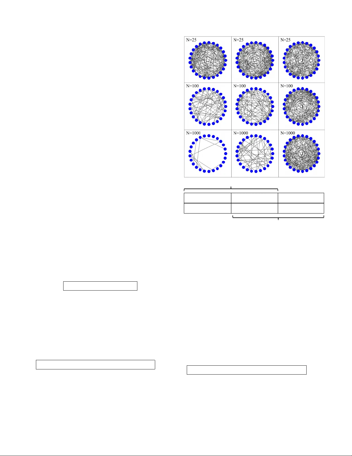
1 Graph Learning Under P artial Observ ability V incenzo Matta, Augusto Santos, and Ali H. Sayed Abstract —Many optimization, inference and learning tasks can be accomplished efﬁciently by means of decentralized processing algorithms where the netw ork topology (i.e., the graph ) plays a critical role in enabling the interactions among neighboring nodes. There is a large body of literature examining the effect of the graph structure on the perf ormance of decentralized pro- cessing strategies. In this article, we examine the in verse problem and consider the r everse question: How much information does observing the behavior at the nodes of a graph con vey about the underlying topology? For large-scale networks, the difﬁculty in addressing such inv erse problems is compounded by the fact that usually only a limited fraction of the nodes can be probed, giving rise to a second important question: Despite the pr esence of unobserved nodes, can partial observations still be sufﬁcient to discover the graph linking the probed nodes? The article surveys recent advances on this challenging learning problem and related questions. Index T erms —Graph lear ning, topology inference, network tomography , Granger estimator , diffusion network, Erd ˝ os-R ´ enyi graph. I . I N T R O D U C T I O N T HIS survey deals with complex systems whose ev olution is dictated by interactions among a large number of elementary units (referred to as network nodes ). The inter- actions giv e rise to some form of decentralized information processing that is characterized by two fundamental features: i ) the locality of information exchange between the individual units; and ii ) the capability to solve rather effecti vely a range of demanding tasks (such as optimization, learning, and inference) that would otherwise be unattainable by stand-alone isolated nodes. There is a large body of literature that examines how the graph topology linking the nodes affects the performance of decentralized processing methods — see, e.g., [1]–[14]. This article focuses on the rev erse question, namely , what informa- tion the optimization solution con ve ys about the underlying topology . Speciﬁcally , assuming that we are able to observe the e volution of the signals at a subset of the nodes, we would like to examine what type of information can be e xtracted from these measurements in relation to the interconnections between the nodes. Rather than focus on what the nodes learn through decen- tralized processing (which is the goal of the direct learning problem), we focus instead on a dual learning problem that V . Matta is with DIEM, Uni versity of Salerno, via Gio vanni Paolo II, I- 84084, Fisciano (SA), Italy (e-mail: vmatta@unisa.it). A. Santos was with the Adaptive System Laboratory , EPFL, CH-1015 Lausanne, Switzerland (e-mail: augusto.pt@gmail.com). A. H. Sayed is with the ´ Ecole Polytechnique F ´ ed ´ erale de Lausanne EPFL, School of Engineering, CH-1015 Lausanne, Switzerland (e-mail: ali.sayed@epﬂ.ch). The work of A. H. Sayed was supported in part by grant 205121-184999 from the Swiss National Science Foundation. Fig. 1. Illustration of the graph learning problem considered in this article. A network performs a decentralized processing task (the dir ect learning prob- lem). The network graph inﬂuences the way each node exchanges information with its neighbors. The online output of the decentralized processing at node k and time i is denoted by y k ( i ) . An inferential engine can probe the subset { j, k, `, m } of the network, and collect the pertinent outputs. Based on these outputs, the goal of the dual learning problem is to estimate the subgraph of connections between nodes j, k , `, m . deals with how the nodes learn (i.e., on discov ering the hidden interconnections that drive the learning process). A schematic illustration of this combined interplay is pro vided in Fig. 1. In the direct problem, we start from a graph topology , run a de- centralized processing algorithm, and analyze its performance (such as con ver gence rate and closeness to optimal solution) and the dependence of this performance on the graph. In the dual problem, we start from observing the signals generated by the nodes and focus instead on discov ering the underlying graph that led to the observed signal e volution. The graph learning problem has man y challenging aspects to it, as we explain below . Nevertheless, it is a problem of fundamental importance arising across a variety of application domains and disciplines 1 because it can provide answers to many useful questions of interest. For instance, by observing the ev olution of signals at a subset of the nodes, can one establish which nodes are sharing information with each other? Or ho w is pri vac y reﬂected in the nodes’ signals? Also, by observing the behavior of some nodes, can one discover which nodes are ha ving a magniﬁed inﬂuence on the overall behavior of the network? Applications that can beneﬁt from such answers are numerous. For example, disco vering who is communicating with whom ov er the Internet [15]–[18]; tracing the information ﬂo w ov er a social network to capture the 1 Since the considered problem arises across multiple disciplines, it is referred to in multiple ways including: graph learning, topology inference, network tomography , graph reconstruction, graph estimation. In the following, we will mostly use “graph learning”. 2 mechanism of opinion formation or to locate the source of f ake news [19], [20]; using graphs to characterize the e volution of urban traf ﬁc [21]; learning the synchronized cogniti ve behavior of a school of ﬁsh ev ading predators [22], [23]; in vestigating the relationship between structural and functional connecti vity in the brain [24]. In this article we focus on netw orks go verned by discr ete- time linear dynamical systems described by Eq. (3) further ahead. This class of models has found application in many do- mains. For e xample, it is a classical model used in economics for time-series forecasting of ﬁnancial data [25]; it has been applied in biostatistics and bioinformatics to estimate gene regulatory networks from gene e xpression data [26]; it arises automatically ov er networks deployed to solve distributed inference tasks, such as distributed detection problems [27], [28]. There e xist some useful surve y articles related to the topic of graph learning [29]–[31]. Howe ver , most prior works assume that all nodes in a network are monitored. This is usually not the case. For example, in probing signals from the brain, only certain localities are examined. Also, in probing signal ﬂows ov er a social network with millions of members, only a limited number of observ ations may be a vailable. It is therefore critical to study how these limitations inﬂuence the problem of graph learning. As such, a core feature of this article is that we deal with lar ge networks. Ov er these networks, due to different forms of physical limitations, it is not practical to assume that data can be collected from all nodes. This is seldom the case and our standing assumption in this presentation will be that observations are collected from only a subset of the nodes. W e refer to this scenario as the partial observability regime. As a result, the graph learning task becomes more complicated than usual, since the observations collected at the monitored nodes are inﬂuenced (through information propagation) by the unobserved nodes. It is then natural to inquire whether this partial observ ability setting leads to an ill-posed graph learning problem or can still provide sufﬁcient information to learn the underlying graph linking the observed nodes. This is a hard problem, which will not be feasible in general. The main aim of this article is to survey some recent advances on graph learning under partial observ ability for networks gov erned by linear dynamical systems. In particular , we will ﬁnd that, despite the (massive, since the network is lar ge) inﬂuence of the latent unobserved nodes , the topology of the monitored subnetwork can be estimated well under proper conditions, and we will illustrate the meaning of these conditions. The roadmap we follow to pursue this goal is as follows. In Sec. II we start by formulating the problem, then in Sec. III we illustrate the main issues in graph learning and how they are dealt with in the literature. W e then focus on some recent theoretical advances in the ﬁeld, which show how graph learning under partial observ ability can be feasible, in a setting that considers random graphs and certain properties of the combination matrix that the nodes employ in the ev olution of the distributed network algorithms — see Sec. IV. Section V is dev oted to illustrating graph learning in operation: ﬁrst we present a distributed detection example; then we use the experiments to highlight useful properties of the graph learning algorithms such as their complexity , performance and ﬁnite- size ef fects; and ﬁnally we sho w ho w an o verall graph can be learned by sequentially reconstructing smaller portions thereof. Conclusions and perspecti ves follow in Sec. VI. Notation . W e use boldface letters to denote random vari- ables, and normal font letters for their realizations. Matrices are denoted by capital letters, and vectors by small letters. This con vention can be occasionally violated, for example, the total number of network nodes is denoted by N . A random vector x that depends on a spatial (i.e., node) index k and a time index i is denoted by x k,i . A (scalar) random variable that depends on a spatial inde x k and a time index i is denoted by x k ( i ) . The symbol p − → denotes con vergence in probability as N → ∞ . When we say that an event occurs “w .h.p. ” we mean that it occurs “with high probability” as N → ∞ . Sets and events are denoted by upper-case calligraphic letters, whereas the corresponding normal font letters will denote set cardinalities. For example, the cardinality of S is S . The complement of S is denoted by S 0 . For a K × K matrix Z , the submatrix spanning the rows of Z indexed by set S ⊆ { 1 , 2 , . . . , K } and the columns indexed by set T ⊆ { 1 , 2 , . . . , K } , is denoted by Z ST , or alternativ ely by [ Z ] ST . When S = T , the submatrix Z ST is abbreviated as Z S . The symbol log denotes the natural logarithm. I I . F O R M U L A T I O N O F T H E P R O B L E M W e are given a connected network of N nodes, which implement a distributed dif fusion algorithm in the form that we are going to illustrate. The output of node k = 1 , 2 , . . . , N at time i ≥ 0 will be henceforth assumed to be a random variable denoted by y k ( i ) . For a gi ven time instant, the outputs of all nodes are stack ed into an N × 1 column vector: y i = [ y 1 ( i ) , y 2 ( i ) , . . . , y N ( i )] > . (1) Like wise, a second random v ariable x k ( i ) will represent the input data (or some function thereof), giving rise to the vector: x i = [ x 1 ( i ) , x 2 ( i ) , . . . , x N ( i )] > . (2) W e assume that the input variables x k ( i ) are independent and identically distrib uted (i.i.d.) both spatially (i.e., across node index k ) and temporally (i.e., over time index i ). W e focus on the follo wing diffusion model, a.k.a. ﬁrst-order V ector AutoRegressi ve (V AR) model, which represents the dif fusion learning process across the network: y i = A y i − 1 + x i (3) Expanding (3) on an entrywise basis we get: y k ( i ) = N X ` =1 a k` y ` ( i − 1) + x k ( i ) . (4) W e see from (4) that the structure of the combination matrix A = [ a k` ] is critical in determining how node k incorporates information coming from node ` . In particular , the sk eleton of A (i.e., the support graph gi ven by the locations of the nonzero entries of A ) encodes the possible paths that the information can follow through during the dif fusion process (4). 3 In the graph learning problem under partial observability , only a limited subset S of nodes can be probed (i.e., their signals { y k ( i ) } k ∈ S observed), and the main goal is to estimate the support graph G S of the submatrix A S (recall that this notation refers to restricting A to the ro ws and columns deﬁned by the indices in S ). The graph learning pipeline can be summarized in the follo wing ﬂow diagram: Y = { y k (1) , y k (2) , . . . , y k ( i ) } k ∈ S | {z } gather signals from S ⇓ b A S = f ( Y ) | {z } estimate the combination submatrix in S ⇓ b G S = h ( b A S ) | {z } estimate the subgraph in S (5) In (5), the function f represents a mapping from the data to an estimated combination submatrix, while the function h is a suitable thr esholding or clustering operator that classiﬁes the entries of b A S as connected/disconnected. According to (5), one fundamental step is to devise a suitable function f to estimate the combination matrix. On ﬁrst thought, it may appear natural to choose f as the cov ari- ance matrix, since one expects that the statistical correlation between the signals at two nodes provides an indication on whether they are connected or not. On closer reﬂection, howe ver , one ﬁnds that this approach is problematic and more effecti ve solutions are necessary . This is because over a connected network with cooperati ve nodes, pairwise corre- lation between two nodes is also affected by data streaming from other nodes through the successive local interactions: Nodes interact with their neighbors, which in turn interact with their neighbors, and so forth. As a result, if node k is connected to ` through an intermediate node m , the outputs of k and ` will be correlated even though there is no direct link between them. For this reason, it is not true in general that the combination matrix entries can be faithfully estimated fr om the corresponding covariance matrix entries. This is true only for special networks that are called correlation networks, but many other possibilities exist. For e xample, in a Gaussian graphical model [32]: i ) the measurements at the network nodes obey a multiv ariate normal distribution with a certain cov ariance matrix; and ii ) the nonzero entries of the inver se of the cov ariance matrix (a.k.a. concentration matrix) correspond to the support graph of the network. But it should be remarked that e ven this result is not general enough, and that effecti ve estimators for the graph must necessarily depend as well on the signal dynamics ov er the graph. The next section focuses on suitable choices for the model in (3). A. Estimating the Combination Matrix A in Model (3) For ease of presentation, in the forthcoming treatment we will assume, without loss of generality , that the random variables { x k ( i ) } in (3) are zero mean and have unit variance. Multiplying both sides of (3) by y > i − 1 and taking expectations, we obtain: E  y i y > i − 1  | {z } i →∞ − → R 1 = A E  y i − 1 y > i − 1  | {z } i →∞ − → R 0 + E [ x i y > i − 1 ] | {z } =0 , (6) where the last term is zero because the sequence { x i } is formed by independent and zero-mean random vectors, and where R 0 and R 1 are the limiting covariance and one-lag cov ariance matrices, respectiv ely (these limits exist if A is a stable matrix) [14]. From (6) we immediately observe that the matrix A can be expressed as: A = R 1 R − 1 0 , (7) which is rele vant for graph learning because cov ariance matri- ces can be estimated from samples, with increasing accurac y as the number of samples increases. The solution in (7) can be interpreted as searching for the coefﬁcients { a k` } that provide the best (in mean-square-error sense) linear prediction of y i giv en the past sample y i − 1 — see, e.g., [33]. Estimator (7) is also kno wn as Granger estimator or predictor , a terminology that arises in the context of Granger causality [34]. 2 Howe ver , in order to ev aluate R 0 and R 1 we need to probe the entire network. Accordingly , estimator (7) is not useful under the partial observability regime adopted here, where only nodes belonging to subset S are probed. One approach to estimate the submatrix A S could be by applying (7) to the cov ariance submatrices pertaining to S : b A S = [ R 1 ] S ([ R 0 ] S ) − 1 . (8) This approach would correspond to determining the coefﬁ- cients { a k` } (for k , ` ∈ S ) that provide the minimum-mean- square-error linear prediction of the subv ector containing the elements of { y k ( i ) } for k ∈ S , giv en the subvector of the past samples { y k ( i − 1) } for k ∈ S . Unfortunately , matrix analysis tells us that [35]: A S =  R 1 R − 1 0  S 6 = [ R 1 ] S ([ R 0 ] S ) − 1 (9) The middle term corresponds to extracting the S component from the product R 1 R − 1 0 , whereas the last term corresponds to ﬁrst extracting the S components from the individual cov ariances R 1 and R 0 . The inequality sign is because the term  R 1 R − 1 0  S takes into account the effect of the latent nodes befor e projection onto the set S . Therefore, a Granger predictor that ignores the latent variables is not necessarily satisfactory . In particular , the elementary result in (9) provides an immediate hint on the fact that the graph learning problem is not necessarily feasible under partial observ ability . I I I . L I T E R A T U R E S U RV E Y It is useful to illustrate three fundamental issues arising in the context of graph learning. 2 In a nutshell, Granger causality refers to the relationships between time se- ries. With reference to our example, assume that we regress y k ( i ) on the past one-lag time series available in the network, y ` ( i − 1) , for ` = 1 , 2 , . . . , N . As we have observed, the optimal predictor minimizing the regression error would not use the time series with a k` = 0 to predict y k ( i ) . Thus, one says that k is “Granger-caused” by those ` for which a k` 6 = 0 . 4 A. Achievability , Hardness, and Sample Complexity I. Achie vability . W e say that graph learning is achiev able when the graph of interest can be estimated well 3 at least in the case of unlimited complexity . In this case, practical complexity constraints are ignored, for example, it is assumed that one can collect as many samples as desired and that the computational complexity associated with matrix inv ersion or search algorithms is not of concern. T o illustrate this concept, consider model (3) under full observability . From (7) we see that graph learning is achiev able since there is a closed-form relationship that allo ws retrie ving A from R 0 and R 1 , and since we assume that the cov ariance matrices can be estimated perfectly from the data for a large number of samples. In our partial observability setting, achie vability is a critical and challenging issue, due to the assumption that we can collect data from only a limited portion of the netw ork, whereas the number of unobserved nodes may scale to inﬁnity . Fortunately , it has been sho wn that, under certain conditions, graph learning with partial observations is achiev able [36]–[39], as we will discuss in Sec. IV. Howe ver , e ven when achiev ability is established, there are at least two other aspects to consider related to har dness and sample complexity . II. Hardness or Computational Complexity . When examin- ing hardness, we continue to disregard the complexity asso- ciated with the number of samples. That is, we continue to assume that an inﬁnite collection of samples is a v ailable, such that no error arises from statistical ﬂuctuations and the statis- tical quantities of interest are perfectly known. The concept of hardness is then related to the computational complexity required to determine the support graph. F or instance, with reference to the model in (3), with inﬁnitely many samples we can assume that R 0 and R 1 are perfectly kno wn. Hence, hardness refers to the computational complexity required to estimate the support graph from R 0 and R 1 , which essentially amounts to inv erting a large matrix. In some other graph learning problems hardness becomes a serious issue, since an NP search would be required to estimate the graph [40]–[44]. III. Sample Comple xity . This concept refers to the number of samples that are required to perform accurate graph learning. It also relates to how the number of necessary samples scales with the dimensionality of the problem (i.e., the network size). The issue of establishing ho w limited sample av ailability affects the learning performance is particularly relev ant in the high-dimensional setting where the number of samples can be signiﬁcantly smaller than the network size, as happens in the theoretical domain of high-dimensional graphical mod- els [32], or in application domains such as gene regulatory networks [26]. It is useful to illustrate the sample complexity issue in relation to problems where one estimates cov ariance matrices (e.g., under Gaussian graphical models or V AR models). Empirical cov ariance matrices are known to be rank deﬁcient when the number of samples is smaller than or equal to the network size, which is clearly a problem when one needs to 3 W e will quantify the qualiﬁcation “well” in Sec. IV -D, where we introduce formal notions of consistency to measure the accuracy of a graph estimate as the network size increases. estimate the concentration matrix (in verse of the cov ariance matrix), or when one needs to compute a Granger estimator like the one in (7). Even when the empirical covariance is not singular , the number of samples necessary to attain satisfactory performance can be large. For example, as we will see later, the nonzero entries of the combination matrix usually become smaller as the network size increases. This means that for large networks, it becomes necessary to increase the accuracy of the empirical covariance matrices. When possible, one may resort to structural constraints (such as sparsity or smoothness) to regularize the estimation of the cov ariance matrices and keep sample complexity under control. One useful technique over sparse graphical models is the graphical LASSO method to estimate the concentration matrix [45]. The majority of results that are av ailable for sample com- plexity in the context of graphical models do not apply to graphs obeying dynamical systems like (3). This is because most of these results assume graphical models with i.i.d. observation samples rather than observations that arise from a dynamical model with memory [30]. Some results on the sample complexity associated with model (3) appear in [46]– [49] but they refer to the setting of full observability . Under partial observability , the issue is considered in [38], [39]. B. Graph Learning Under Full Observability Owing to the nature of model (3), we will mainly focus on linear system dynamics, but hasten to add that there exist works on graph learning ov er nonlinear dynamical systems as well [29], [50]–[55]. One useful work on graph learning over linear systems is [56], which considers a fairly general class of models (including non-causal systems and V AR models of any order). The main contribution of [56] is to devise an inferential strat- egy relying on W iener ﬁltering to retrie ve the network graph. Such strategy is shown to guarantee exact reconstruction for the so-called self-kin networks. For more general network structures, the reconstruction of the smallest self-kin network embodying the true network is guaranteed. In the context of graph signal processing [57]–[61], recent works focus on autoregressiv e diffusion models of arbitrary order [62]–[64]. As a common feature of many of these works, the estimation algorithms lev erage some prior kno wl- edge about the graph structure, which is then translated into appropriate structural constraints. T ypical constraints are in terms of sparsity of the connections, or smoothness (in the graph signal terminology) of the signals deﬁned at the graph nodes. In [62], a two-step inferential process is proposed, where: i ) a graph shift operator [65]–[67] is estimated through the nodes’ signals that arise from the diffusion process; and ii ) giv en the spectral templates obtained from this estimation, the eigen v alues that would identify the graph are then estimated by adding proper structural constraints (e.g., sparsity) that could render the problem well-posed. In [63], the same concept of a two-step procedure is considered, with the main goal being to characterize the space of v alid graphs, namely , graphs that can explain the signals measured at the network nodes. In [64], a model for causal gr aph pr ocesses is proposed, which exploits 5 both inter-relations among nodes’ signals and their intra- relations across time. Capitalizing on these relations, a viable algorithm for graph structure recovery is designed, which is shown to con ver ge under reasonable technical assumptions. There also exist works on graph learning o ver other types of dynamical systems. In [68], a graphical model is pro- posed to represent networks of stochastic processes. Under suitable technical conditions, it is shown that such graphs are consistent with dir ected information graphs , which are based on a generalization of Granger causality . It is proved how directed information quantiﬁes causality in a speciﬁc sense and efﬁcient algorithms are de vised to estimate the topology from the data. In [69], a novel measure of causality is introduced, which is able to capture functional dependencies exhibited by certain (possibly nonlinear) network dynamical systems. These dependencies are then encoded in a functional dependency graph, which becomes a representation of possibly directed (i.e., causal) inﬂuences that are more sophisticated than the classical types of inﬂuences encoded in linear network dynamical systems. Results for graph learning ov er continuous-time linear dy- namical systems described by stochastic dif ferential equations are provided in [46]. Conditions to achie ve consistent graph learning are of fered, along with a sample complexity anal- ysis that relies on concentration bounds for the empirical cov ariance matrix. A least-squares algorithm with ` 1 -norm regularization is proposed. The analysis in [46] goes through a discretization of the model, which can be relevant also to the analysis of discrete-time diffusion models like the one in (3). For these latter models, achiev ability of consistent graph learning over sparse graphs is examined in [49]. An algorithm is designed, which tries to ﬁt (6) with the most sparse matrix possible. Some generalizations of this result to the case of missing observations are offered in [47], [48], where samples from the entire network are gathered, but the y can be intermittently av ailable, or corrupted (these av ailable observations are called “partial observations”, but the meaning is dif ferent from the one adopted in this article, since in [47], [48] all nodes are probed, and the qualiﬁcation “partial” refers to intermittence of observ ations at each node). In summary , the aforementioned works (which we list with no pretense of exhaustiv eness) address under various settings the problem of achie vability and complexity of graph learning under the full observ ability regime. Ho we ver , we must recall that in our setting we focus on the partial observability regime where a large portion of the network is not accessible. Most challenges in terms of feasibility of the graph learning problem will in f act stem from this complication. C. Graph Learning under P artial Observability In the presence of unobserved network nodes, there are results allowing proper graph learning when the topology is of some pre-assigned type (polytrees) [70], [71]. F or fairly arbitrary graph structures, some results about the possibility of correct graph retrie val are provided in [72], [73]. One limitation of these results resides in the f act that the suf ﬁcient conditions for graph learning depend on some “microscopic” details about the model (e.g., about the local structure of the topology or the pertinent statistical model). For this reason, ov er large-scale netw orks (which are the focus of this article) a different approach is necessary . One approach suited to large networks is an asymptotic analysis carried out as the network size N scales to inﬁnity . In order to cope with the lar ge network size in a way that enables a tractable analysis, it is useful to model the network graph as a random graph. An asymptotic analysis can then become feasible, letting emer ge the thermodynamic properties of the graph, with the conditions for graph learning being summarized in some macr oscopic (i.e., average) indicators, such as the probability that two nodes of the random graph are connected. Similar forms of asymptotic analysis were recently per- formed for high-dimensional graphical models with latent variables. In [74], the focus is on Gaussian graphical models, and consistent graph learning is prov ed (along with a viable algorithmic solution) under an appropriate local separation criterion . In [75] results of consistent learning are instead provided for locally tree-lik e graphs. Graph learning under the so-termed “ sparsity+low-rank ” condition is examined in [76]. Under this condition (where the observed subnetwork is sparse and the unobserved subnetwork is low-rank in an appropriate sense), it is proved that the graph and the amount of latent variables can be jointly estimated. Moreover , in [74]–[76], a detailed analysis of sample complexity is provided, which is especially rele vant since these works focus on the high- dimensional setting where the number of samples can be smaller than the network size. In [77], a graphical model consisting of a ferromagnetic restricted Boltzmann machine with bounded degree is considered. It is shown that such class of graphical models can be effecti vely learned through the usage of a nov el inﬂuence-maximization metric. Howe ver , classical graphical models (such as the ones used in the aforementioned references) do not assume that there are signals evolving ov er time at the network nodes. In contrast, classical graphical models assume a still picture of the network, where the data measured at the individual nodes are modeled as random v ariables characterized by a certain joint distribution. The inter-node statistical dependencies are encoded in the joint distribution through an underlying graph. Under this framework, estimation of the graph from the data deﬁned at the nodes is performed assuming that the inferential engine has access to i.i.d. samples of these data, and there is no model of the ev olution of the data across time. For this reason, the results obtained in the aforementioned references on graph learning in the presence of latent variables do not apply to the dynamical system considered in (3). Results relev ant to the latter system are provided in [39], start- ing from the “ spar sity+low-rank ” approach proposed in [76]. In [39] it is assumed that the probed subgraph is sparse, and that a certain matrix associated with the unobserved nodes is low-rank, which in particular means that the number of unobserved nodes must be smaller than the number of probed ones. In order to ﬁt (3), a regularized least-squares algorithm is proposed, where ` 1 -norm regularization is used to control sparsity , and nuclear-norm regularization to control the rank 6 of the matrix associated with the latent network part. Exploiting the properties of Erd ˝ os-R ´ enyi (ER) random graphs and the regularity of the combination matrices used in typical distributed processing settings, some recent ad- vances provide examples of achiev able graph learning under partial observability when the graph of probed nodes is not necessarily sparse, and the number of latent nodes can be arbitrarily large [36]–[38], [78]–[82]. The forthcoming section summarizes these adv ances in some detail. I V . A C H I E V A B L E G R A P H L E A R N I N G As e xplained in the previous section, for large netw orks it is necessary to perform some asymptotic analysis to obtain useful analytical results, and to establish the fundamental thermodynamic properties that emerge with high probability ov er the network. One typical way to tackle this problem is to randomize the network structure, i.e., to work with r andom graphs . One useful class of random graphs is the celebrated model proposed by Erd ˝ os and R ´ enyi [83], [84], which is an undirected graph where the probability that nodes k and ` are connected is a Bernoulli random variable characterized by a certain connection probability p , and where all edges are drawn independently and with the same connection probability . An important graph descriptor is the de gr ee of a node. The degree of node k is deﬁned as the number of neighbors of node k (including k itself), and will be denoted by d k . Owing to the Bernoulli model, the av erage degree D av of e very node in an Erd ˝ os-R ´ enyi graph is equal to 1 + ( N − 1) p . A. Graph Evolution Re gimes Let us examine the ev olution of the random graph when N grows. When the connection probability is a constant p > 0 , the number of neighbors increases linearly with N (in the following, the notation ∼ means “scales as”, when N → ∞ ): D av ∼ N p [dense regime] (10) It is not difﬁcult to ﬁgure out that, since in this case any node has a number of neighbors growing as N , the graph exhibits a dense connection structure, and for sufﬁciently lar ge N , is likely to be a connected graph, i.e., a graph where there always exists an undirected path connecting any pair of nodes. Ho we ver , a fundamental result from random graph theory states that, in order to ensure a graph is connected with high probability as N grows, the minimal growth of the av erage degree is [83], [84]: D av = log N + O (log N ) [log-sparse re gime] (11) where by O (log N ) we denote a sequence that div erges 4 to + ∞ at most logarithmically and, hence, the connection probability p ∼ D av / N vanishes. The logarithmic growth corresponds in fact to a phase transition , since it represents the minimal gro wth that ensures a connected graph. 4 The Big-O notation f ( N ) = O ( g ( N )) usually means that | f ( N ) | is upper bounded by c | g ( N ) | for some constant c and sufﬁciently large N . Our notation O ( f ( N )) adds the requirement that f ( N ) → + ∞ as N → ∞ . ! ! ! ! regime&of& "#$%&'(!)&#)*#+',-&# &of°rees& . /,'.*! regime& 7 our setting (e.g., re gularity of the combination matrices used for the distrib uted optimization algorithm), more po werful results can be obtained. F or instance, we will see that, dif ferent from what happens in other conte xts, our problem can be- come feasible also for densely connected netw orks. F or these models, results for graph learning under partial observ ation ha v e been recently obtained in [18], [19], [59]–[61]. In the follo wing, we will present these recent adv ances in some detail. Notation . W e use boldf ace letters to denote random v ari- ables, and normal font letters for their realizat ions. Matrices are denoted by capital letters, and v ectors by small letters. This con v ention can be occasionally violated, for e xample, the total number of netw ork nodes is denoted by N . The symbol p ! denotes con v er gence in probability as N ! 1 . When we say that an e v ent occurs “w .h.p. ” we mean that it occurs “with high probability” as N !1 . Sets and e v ents are denoted by upper -case calligraphic letters, whereas the corresponding normal font letter will denote the set cardinality . F or e xample, the ca rdinality of S is S . The complement of S is denoted by S 0 . F or a K ⇥ K matrix Z , the submatrix spanning the ro ws of Z inde x ed by set S ✓ { 1 , 2 ,. .., K } and the columns inde x ed by set T ✓ { 1 , 2 ,. .., K } , is denoted by Z ST , or alternati v ely by [ Z ] ST . Whe n S = T , t he submatrix Z ST is abbre viated as Z S . Moreo v er , in the inde xing of the submatrix we k eep the inde x set of the original matrix. F or e xample, if S = { 2 , 3 } and T = { 2 , 4 , 5 } , the submatrix M = Z ST is a 2 ⇥ 3 matrix, inde x ed as follo ws: M = ✓ z 22 z 24 z 25 z 32 z 34 z 35 ◆ = ✓ m 22 m 24 m 25 m 32 m 34 m 35 ◆ . (24) The symbol l og denotes the natural log arithm. V. R AND OM G RAP H M OD EL As said in the pre vious section, o v er lar ge netw orks it is necessary to perform some asymptotic analysis to obtain useful analytical results, and to establish the fundamental thermodynamic properties that emer ge with high probability o v er the netw ork. The typical w ay to tackle this problem is to w ork with r andom netw ork structure, i.e., with r andom gr aphs . One useful class of random graphs is the celebrated model proposed by Erd ˝ os and R ´ en yi, which is an (undirected) graph where the probability that nodes i and j are connected is a Bernoulli random v ariable characterized by a certain connection probability p , and where all edges are dra wn independently and with the same connection probability [80], [81]. Owing to the Bernoulli model, the a v erage de gree D av (i.e., the e xpected number of neighbors including the node itself) of e v ery node of the Erd ˝ os-R ´ en yi (ER) graph is equal to 1+ ( N  1) p . Let us no w focus on the e v olution of the random graph when N gro ws. When the connection probability is a constant p> 0 , the number of neighbors increases linearly with N . It is not dif ﬁcult to ﬁgure out that, since in this case an y node has a number of neighbors gro wing as N , the graph e xhibits a dense connection structure, and for suf ﬁciently lar ge N , is lik ely to be a connected graph, i.e., a graph where co n ce n t ra t i o n re g i me sp a rsi t y re g i me ve ry sp a rse u n i f o rm & sp a rse u n i f o rm & d e n se Fig. 2. V enn diagram illustrating the relationships between concentration and sparsity o v er a connected Erd ˝ os-R ´ en yi graph. there al w ays e xists an (undirected) path connecting an y pair of nodes: D av ⇠ Np [dense re gime] (25) Ho we v er , a fundamental result of random graph theory states that, in order to see a graph connected with high probability as N gro ws, it is suf ﬁcient that the a v erage de gree g r o ws log arithmically with N , formally: D av = l og N + O ( l og N ) [log-sparse re gime] (26) where O ( l og N ) is a sequence di v er ging to + 1 at most log arithmically and, hence, the connection probability D av /N v anishes. The log arithmic gro wth corresponds in f act to a phase transition, in the sense that is the minimal gro wth that ensures a connected graph. There is yet a third (sparse) connected re gime, which is intermediate between the log-sparse and the dense re gimes occurs when the a v erage de gree gro ws f aster than log arithmi- cally (while the connection probability still v anishes), formally when: D av = ! N l og N [intermediate-sparse re gime] (27) where ! N !1 in an arbitrary f ashion, b ut suf ﬁciently slo w so as to ensure that the connection probability D av /N v anishes. There is one fundamental property that holds under the sparse and dense re gimes, b ut not under the log-sparse re gime, and is the follo wing statistical concentr ation of the minimal and maximal de grees of the graph: 1 d min D av p ! 1 , d max D av p ! 1 , [uniform concentration] (28) which means that, under (27), the minimal and maximal de gree concentrate around the e xpected de gree. The o v erall taxonomy comprising the dif ferent elements of sparsity , density , and de- gree concentration, is reported in Fig. 2. W e see that the union of the log-sparse and intermediate-sparse re gimes identiﬁes the sparse (as opposed to the dense) re gim e. Lik e wise, the union of the intermediate-sparse and dense re gimes identiﬁes the re gime of de gree concentration. 1 W e note that the term “concentration” does not refer to the number of node connections, b ut, according to a standard terminology adopted in statistics, will be used to refer to statistical quantities that collapse to som e deterministic v alue as N !1 [82]. 7 our setting (e.g., re gularity of the combination matrices used for the distrib uted optimization algorithm), more po werful results can be obtained. F or instance, we will see that, dif ferent from what happens in other conte xts, our problem can be- come feasible also for densely connected netw orks. F or these models, results for graph learning under partial observ ation ha v e been recently obtained in [18], [19], [59]–[61]. In the follo wing, we will present these recent adv ances in some detail. Notation . W e use boldf ace letters to denote random v ari- ables, and normal font letters for their realizat ions. Matrices are denoted by capital letters, and v ectors by small letters. This con v ention can be occasionally violated, for e xample, the total number of netw ork nodes is denoted by N . The symbol p ! denotes con v er gence in probability as N ! 1 . When we say that an e v ent occurs “w .h.p. ” we mean that it occurs “with high probability” as N !1 . Sets and e v ents are denoted by upper -case calligraphic letters, whereas the corresponding normal font letter will denote the set cardinality . F or e xample, the ca rdinality of S is S . The complement of S is denoted by S 0 . F or a K ⇥ K matrix Z , the submatrix spanning the ro ws of Z inde x ed by set S ✓ { 1 , 2 ,. .., K } and the columns inde x ed by set T ✓ { 1 , 2 ,. .., K } , is denoted by Z ST , or alternati v ely by [ Z ] ST . Whe n S = T , t he submatrix Z ST is abbre viated as Z S . Moreo v er , in the inde xing of the submatrix we k eep the inde x set of the original matrix. F or e xample, if S = { 2 , 3 } and T = { 2 , 4 , 5 } , the submatrix M = Z ST is a 2 ⇥ 3 matrix, inde x ed as follo ws: M = ✓ z 22 z 24 z 25 z 32 z 34 z 35 ◆ = ✓ m 22 m 24 m 25 m 32 m 34 m 35 ◆ . (24) The symbol l og denotes the natural log arithm. V. R AND OM G RAP H M OD EL As said in the pre vious section, o v er lar ge netw orks it is necessary to perform some asymptotic analysis to obtain useful analytical results, and to establish the fundamental thermodynamic properties that emer ge with high probability o v er the netw ork. The typical w ay to tackle this problem is to w ork with r andom netw ork structure, i.e., with r andom gr aphs . One useful class of random graphs is the celebrated model proposed by Erd ˝ os and R ´ en yi, which is an (undirected) graph where the probability that nodes i and j are connected is a Bernoulli random v ariable characterized by a certain connection probability p , and where all edges are dra wn independently and with the same connection probability [80], [81]. Owing to the Bernoulli model, the a v erage de gree D av (i.e., the e xpected number of neighbors including the node itself) of e v ery node of the Erd ˝ os-R ´ en yi (ER) graph is equal to 1+ ( N  1) p . Let us no w focus on the e v olution of the random graph when N gro ws. When the connection probability is a constant p> 0 , the number of neighbors increases linearly with N . It is not dif ﬁcult to ﬁgure out that, since in this case an y node has a number of neighbors gro wing as N , the graph e xhibits a dense connection structure, and for suf ﬁciently lar ge N , is lik ely to be a connected graph, i.e., a graph where co n ce n t ra t i o n re g i me sp a rsi t y re g i me ve ry sp a rse u n i f o rm & sp a rse u n i f o rm & d e n se Fig. 2. V enn diagram illustrating the relationships between concentration and sparsity o v er a connected Erd ˝ os-R ´ en yi graph. there al w ays e xists an (undirected) path connecting an y pair of nodes: D av ⇠ Np [dense re gime] (25) Ho we v er , a fundamental result of random graph theory states that, in order to see a graph connected with high probability as N gro ws, it is suf ﬁcient that the a v erage de gree g r o ws log arithmically with N , formally: D av = log N + O (log N ) [log-sparse re gime] (26) where O ( l og N ) is a sequence di v er ging to + 1 at most log arithmically and, hence, the connection probability D av /N v anishes. The log arithmic gro wth corresponds in f act to a phase transition, in the sense that is the minimal gro wth that ensures a connected graph. There is yet a third (sparse) connected re gime, which is intermediate between the log-sparse and the dense re gimes occurs when the a v erage de gree gro ws f aster than log arithmi- cally (while the connection probability still v anishes), formally when: D av = ! N l og N [intermediate-sparse re gime] (27) where ! N !1 in an arbitrary f ashion, b ut suf ﬁciently slo w so as to ensure that the connection probability D av /N v anishes. There is one fundamental property that holds under the sparse and dense re gimes, b ut not under the log-sparse re gime, and is the follo wing statistical concentr ation of the minimal and maximal de grees of the graph: 1 d min D av p ! 1 , d max D av p ! 1 , [uniform concentration] (28) which means that, under (27), the minimal and maximal de gree concentrate around the e xpected de gree. The o v erall taxonomy comprising the dif ferent elements of sparsity , density , and de- gree concentration, is reported in Fig. 2. W e see that the union of the log-sparse and intermediate-sparse re gimes identiﬁes the sparse (as opposed to the dense) re gim e. Lik e wise, the union of the intermediate-sparse and dense re gimes identiﬁes the re gime of de gree concentration. 1 W e note that the term “concentration” does not refer to the number of node connections, b ut, according to a standard terminology adopted in statistics, will be used to refer to statistical quantities that collapse to som e deterministic v alue as N !1 [82]. 7 our setting (e.g., re gularity of the combination matrices used for the distrib uted optimization algorithm), more po werful results can be obtained. F or instance, we will see that, dif ferent from what happens in other conte xts, our problem can be- come feasible also for densely connected netw orks. F or these models, results for graph learning under partial observ ation ha v e been recently obtained in [18], [19], [59]–[61]. In the follo wing, we will present these recent adv ances in some detail. Notation . W e use boldf ace letters to denote random v ari- ables, and normal font letters for their realizat ions. Matrices are denoted by capital letters, and v ectors by small letters. This con v ention can be occasionally violated, for e xample, the total number of netw ork nodes is denoted by N . The symbol p ! denotes con v er gence in probability as N ! 1 . When we say that an e v ent occurs “w .h.p. ” we mean that it occurs “with high probability” as N !1 . Sets and e v ents are denoted by upper -case calligraphic letters, whereas the corresponding normal font letter will denote the set cardinality . F or e xample, the ca rdinality of S is S . The complement of S is denoted by S 0 . F or a K ⇥ K matrix Z , the submatrix spanning the ro ws of Z inde x ed by set S ✓ { 1 , 2 ,. .., K } and the columns inde x ed by set T ✓ { 1 , 2 ,. .., K } , is denoted by Z ST , or alternati v ely by [ Z ] ST . Whe n S = T , t he submatrix Z ST is abbre viated as Z S . Moreo v er , in the inde xing of the submatrix we k eep the inde x set of the original matrix. F or e xample, if S = { 2 , 3 } and T = { 2 , 4 , 5 } , the submatrix M = Z ST is a 2 ⇥ 3 matrix, inde x ed as follo ws: M = ✓ z 22 z 24 z 25 z 32 z 34 z 35 ◆ = ✓ m 22 m 24 m 25 m 32 m 34 m 35 ◆ . (24) The symbol l og denotes the natural log arithm. V. R AND OM G RAP H M OD EL As said in the pre vious section, o v er lar ge netw orks it is necessary to perform some asymptotic analysis to obtain useful analytical results, and to establish the fundamental thermodynamic properties that emer ge with high probability o v er the netw ork. The typical w ay to tackle this problem is to w ork with r andom netw ork structure, i.e., with r andom gr aphs . One useful class of random graphs is the celebrated model proposed by Erd ˝ os and R ´ en yi, which is an (undirected) graph where the probability that nodes i and j are connected is a Bernoulli random v ariable characterized by a certain connection probability p , and where all edges are dra wn independently and with the same connection probability [80], [81]. Owing to the Bernoulli model, the a v erage de gree D av (i.e., the e xpected number of neighbors including the node itself) of e v ery node of the Erd ˝ os-R ´ en yi (ER) graph is equal to 1+ ( N  1) p . Let us no w focus on the e v olution of the random graph when N gro ws. When the connection probability is a constant p> 0 , the number of neighbors increases linearly with N . It is not dif ﬁcult to ﬁgure out that, since in this case an y node has a number of neighbors gro wing as N , the graph e xhibits a dense connection structure, and for suf ﬁciently lar ge N , is lik ely to be a connected graph, i.e., a graph where co n ce n t ra t i o n re g i me sp a rsi t y re g i me ve ry sp a rse u n i f o rm & sp a rse u n i f o rm & d e n se Fig. 2. V enn diagram illustrating the relationships between concentration and sparsity o v er a connected Erd ˝ os-R ´ en yi graph. there al w ays e xists an (undirected) path connecting an y pair of nodes: D av ⇠ Np [dense re gime] (25) Ho we v er , a fundamental result of random graph theory states that, in order to see a graph connected with high probability as N gro ws, it is suf ﬁcient that the a v erage de gree g r o ws log arithmically with N , formally: D av = l og N + O ( l og N ) [log-sparse re gime] (26) where O ( l og N ) is a sequence di v er ging to + 1 at most log arithmically and, hence, the connection probability D av /N v anishes. The log arithmic gro wth corresponds in f act to a phase transition, in the sense that is the minimal gro wth that ensures a connected graph. There is yet a third (sparse) connected re gime, which is intermediate between the log-sparse and the dense re gimes occurs when the a v erage de gree gro ws f aster than log arithmi- cally (while the connection probability still v anishes), formally when: D av = ! N log N [intermediate-sparse re gime] (27) where ! N !1 in an arbitrary f ashion, b ut suf ﬁciently slo w so as to ensure that the connection probability D av /N v anishes. There is one fundamental property that holds under the sparse and dense re gimes, b ut not under the log-sparse re gime, and is the follo wing statistical concentr ation of the minimal and maximal de grees of the graph: 1 d min D av p ! 1 , d max D av p ! 1 , [uniform concentration] (28) which means that, under (27), the minimal and maximal de gree concentrate around the e xpected de gree. The o v erall taxonomy comprising the dif ferent elements of sparsity , density , and de- gree concentration, is reported in Fig. 2. W e see that the union of the log-sparse and intermediate-sparse re gimes identiﬁes the sparse (as opposed to the dense) re gim e. Lik e wise, the union of the intermediate-sparse and dense re gimes identiﬁes the re gime of de gree concentration. 1 W e note that the term “concentration” does not refer to the number of node connections, b ut, according to a standard terminology adopted in statistics, will be used to refer to statistical quantities that collapse to som e deterministic v alue as N !1 [82]. $#+*'(*0$,+*1./,'.*!'*2$(* & 0*#.*!'*2$(* & 3&21./,'.*!'*2$(* & Fig. 2. T axonomy of the connected regimes for the ER model. The overall sparse regime is given by the union of the log-sparse and intermediate- sparse regimes. In comparison, the union of the intermediate-sparse and dense regimes gi ves rise to the uniform concentration of degr ees , which will be seen to play an important role in the graph learning problem addressed in this article. Each column of the plot grid corresponds to a different regime, from left to right: sparse, intermediate-sparse, and dense, respectiv ely . Moving across ro ws, we consider networks of increasing (from top to bottom) total number of nodes N . For clarity of visualization, in all panels we display only the subgraph of the ﬁrst 25 nodes of the network. There is yet a third (sparse) connected regime, which is intermediate between the log-sparse and the dense regimes introduced so far . This intermediate regime occurs when the av erage degree gro ws f aster than logarithmically (while the connection probability still v anishes), formally when: D av = ω N log N [intermediate-sparse regime] (12) where ω N → ∞ in an arbitrary f ashion, b ut sufﬁciently slow so as to ensure that the connection probability vanishes. There is one fundamental property that holds under the intermediate-sparse and dense regimes, b ut not under the log- sparse regime, and is the following statistical concentration 7 property: 5 d min D av p − → 1 , d max D av p − → 1 , [uniform degree concentration] (13) where d min and d max denote the minimal and maximal degree ov er all nodes, respecti vely . This means that, under (13), the minimal and maximal degree concentrate around the expected degree. The ov erall taxonomy comprising the different elements of sparsity , density , and degree concentration, is reported in Fig. 2, along with an example of ev olution, as N grows, of the ER graphs corresponding to the different regimes. For each regime, we consider an ER graph of increasing size ( N = 25 , 100 , 1000 ), and for each value of N we display (for clarity of visualization) the beha vior of the ﬁrst 25 nodes of the network. For all regimes we start with a connection probability equal to 1 / 2 . Accordingly , the top panels have similar shape. Then, as N increases, the connection probability obeys the scaling law relati ve to the particular regime. In the leftmost panels (sparse regime), we see that the displayed subgraph becomes progressi vely more sparse. 6 In the middle panels (intermediate-sparse regime), sparsity increases, but some more structure is preserved. Finally , in the rightmost panels (dense regime), the subgraph has an in variant behavior . W e see that the union of the log-sparse and intermediate- sparse regimes identiﬁes the sparse (as opposed to the dense) regime. Like wise, the union of the intermediate-sparse and dense regimes identiﬁes the regime of uniform degree con- centration. B. P artial Observability Settings The main challenge of the graph learning problem consid- ered in this article is related to the partial observability setting, where only a subset S of the network can be probed. In order to deal with the asymptotic regime, it is necessary to deﬁne how the cardinality S scales with the o verall network size N . In particular , we introduce the asymptotic fraction of pr obed nodes ξ : S N N →∞ − → ξ (14) The extreme case where the cardinality of probed nodes is ﬁxed when N → ∞ corresponds to a low-observability regime ( ξ = 0 ) where the set of unobserved nodes becomes dominant and inﬁnitely larger than the subset of probed nodes. Howe ver , when the size of S is ﬁxed and ﬁnite, it is not useful to model the connections within S through an ER model because, in the sparse regime, e very edge in S would trivially disappear as N gets large! 5 W e note that the term “concentration” does not refer to the number of node connections, but, according to a standard terminology adopted in statistics, refers to statistical quantities that collapse to some deterministic value as N → ∞ [85]. 6 W e remark that the ov erall graph, which is too large to be displayed, remains connected e ven if the shown subgraph becomes progressiv ely dis- connected. In fact, on the overall graph with N nodes, we can le verage the increasing number of nodes to ﬁnd a path between any two nodes (with high probability) provided that the connection probability scales appropriately . ER model 20% of the total nodes are probed partial ER model 4 nodes are probed N=20 S=4 N=40 S=8 N=20 S=4 N=40 S=4 Fig. 3. Partial observability settings considered in this article. The probed nodes forming the subgraph of interest are highlighted in blue. The evolution for the plain ER regime is illustrated in the top panels. Here, as the network size grows (from N = 20 to N = 40 ), the number of probed nodes grows as well, with the fraction of probed nodes ξ = S/ N = 0 . 2 staying constant and with the subgraph of probed nodes varying. The partial ER regime is illustrated in the bottom panels. Here, the number of probed nodes stays constant ( S = 4 ) as the network size grows and the structure of the probed subgraph is deterministically ﬁxed. In order to deal with the graph learning problem under the low-observ ability regime in a meaningful way , the follo wing partial ER model was introduced in [37]: i ) the subgraph of interest, S , is deterministic and arbitrary ; ii ) while the latent nodes act as a noisy disturbance, with the connections outside S , and also between S and S 0 (the set of latent nodes), dra wn according to an ER model. The distinction between the plain and partial ER models is illustrated in Fig. 3. In the top panels, a plain ER model with ξ = 0 . 2 is considered. W e see that the subset S of probed nodes (displayed in blue) increases from S = 4 to S = 8 when N increases from 20 to 40 . Moreover , the subgraph associated with S (as well as the o verall graph) changes randomly its shape according to an ER model. In comparison, the partial ER model is displayed in the bottom panels. In this case, the subset S of probed nodes has ﬁxed cardinality and structure. The edges (displayed in gray) between nodes belonging to the unobserved set S 0 , as well as between S 0 and S , are randomly drawn according to an ER model. C. Combination Matrices In the presence of partial observations, the graph learning problem can be ill-posed. In fact, while under full observ ability Eq. (7) guarantees that our inv erse problem can be solved, under partial observ ability Eq. (9) highlights that in vertibility is lost due to the error introduced by unobserved nodes, and in general there are no guarantees that this error can allow accurate graph estimation. It makes sense to inv estigate whether it can for certain classes of combination matrices. In the follo wing treatment, the matrix A will be assumed to be symmetric and a scaled (stable) version of a doubly-stochastic matrix, namely , A = A > , a k` ≥ 0 , N X ` =1 a k` = ρ, 0 < ρ < 1 (15) 8 This structure is motiv ated by the typical implementation of combination matrices employed in distributed optimization and learning strategies, for example in consensus [86], [87], gossip algorithms [88], [89], or diffusion algorithms [10]–[14]. In these distributed implementations, if node k is connected to node ` , it scales the output receiv ed from ` through some nonnegati ve weight a k` . In order to perform a distrib uted av eraging, the weight sums are usually kept constant, as in (15). W e will examine an example of these distributed implementations in the detection application considered in Sec. V -A. One useful qualiﬁcation of the combination matrices in (15) that is rele vant to graph learning is in terms of the variability of their nonzero entries. W e introduce two pertinent classes for these matrices. Assumption 1 (Class V 1 ) . The nonzer o entries of the combi- nation matrix, scaled by the avera ge de gr ee D av , do not vanish, namely , given that k and ` ar e connected, a certain θ > 0 exists such that, with high pr obability for lar ge N : D av a k` > θ (16)  Condition (16) is motiv ated by the following observation. For typical choices of combination matrices, each node k distributes the weight mass ρ across its neighbors. Thus, we will have typically , over connected pairs ( k , ` ) : a k` ∝ 1 D av , (17) which explains wh y the quantity D av a k` does not v anish, and why condition (16) is meaningful. Assumption 2 (Class V 2 ) . W e assume that, for connected pairs k and ` : κ d max ≤ a k` ≤ κ d min (18) for some 0 < κ ≤ ρ .  W e see from (18) that, when an edge exists connecting k and ` , the v ariation of the (nonzero) matrix entries is deﬁned in terms of the (reciprocal of the) maximal and minimal graph degrees. Also this condition can be motiv ated by the observation that nodes tend to distrib ute the weights across their neighbors in some homogeneous way . It is possible to sho w that, under the connectivity regimes for the ER model considered here, the left inequality in (18) implies (16), namely , we can conclude that [36]: V 2 ⊂ V 1 . (19) That is, the conditions for a matrix to be in class V 2 are more stringent than the conditions required to be in class V 1 . As a matter of fact, the most popular combination matrices used in distributed processing belong to class V 2 and, hence, to V 1 . T wo notable instances are the Laplacian and Metropolis combination rules, which can be deﬁned as follo ws [14]. For k 6 = ` , with k and ` connected: a k` = αρ d max , [Laplacian rule] a k` = ρ max { d k , d ` } , [Metropolis rule] (20) For both rules, the self-weights are determined by the third condition in (15), yielding a kk = ρ − P ` 6 = k a k` . For the Laplacian rule, the parameter α satisﬁes 0 < α ≤ 1 . D. Consistent Gr aph Learning In the follo wing, the term “consistency” refers to the pos- sibility of learning the graph correctly as N → ∞ . W e will see that dif ferent notions of consistenc y are possible. W e start from the weak est one. W e denote by b A S a certain estimate for the combination (sub)matrix corresponding to subset S . W e explain in the next section sev eral ways by which such an estimate can be computed. W e remark that the consistency results presented next in Sec. IV -F will hold for (plain or partial) ER graphs and symmetric combination matrices. Nevertheless, it is useful to formulate the general theory to handle more general types of graphs (also dir ected ) and asymmetric combination matrices. For this reason, when we refer to node pairs we will actually mean order ed pairs, with ( k , ` ) being distinct from ( `, k ) , because a dir ected link could exist from ` to k and not vice versa. W e ﬁrst introduce a general thresholding rule to classify connected/disconnected pairs. W e will declare that the ordered ( k , ` ) pair is connected (i.e., that the ( k , ` ) entry of the true combination matrix is nonzero) if the corresponding estimated matrix entry , b a k` , exceeds some threshold τ . Accordingly , let us introduce the follo wing error quantities: E 0 ( τ ) , no. of entries where a k` = 0 and b a k` > τ no. of entries where a k` = 0 , E 1 ( τ ) , no. of entries where a k` > 0 and b a k` ≤ τ no. of entries where a k` > 0 , (21) where we assume ( k , ` ) ∈ S with k 6 = ` . More informally , Eqs. (21) can be rephrased as: E 0 ( τ ) , no. of mistak enly classiﬁed disconnected pairs no. of disconnected pairs , E 1 ( τ ) , no. of mistak enly classiﬁed connected pairs no. of connected pairs . (22) Deﬁnition 1 (W eak Consistency) . Let b A S be a matrix estima- tor . W e say that b A S achie ves weak consistency if ther e exists a threshold τ (possibly depending on N ) such that: E 0 ( τ ) + E 1 ( τ ) p − → 0 (23)  The notion of consistency in (23) ensures that the av- erag e fraction of mistakenly classiﬁed edges goes to zero. 9 When the cardinality S of probed nodes is ﬁxed (as happens in the lo w-observ ability regime with partial ER model), an av erage number of mistakes that goes to zero implies that the subgraph of S is perfectly recov ered. In contrast, when the cardinality S grows with N , ensuring a small average fraction of mistakes can be unsatisfactory , which motiv ates the qualiﬁcation “weak”. Let us clarify this issue through a simple example. Consider a reconstruction that is perfect, e xcept for 100 edges that are estimated by the learning algorithm but that are actually not present in the true graph. The a verage number of mistakes, 100 /S , goes to zero as the subnetwork size S goes to inﬁnity , but due to the 100 spurious edges, we will never end up with perfect reconstruction. The presence of (e ven a small number of) spurious edges can be penalizing especially under the sparse re gime, where the number of true edges is small, and a reconstructed network where the number of spurious edges is comparable with the number of true edges might be unsatisf actory . From these observations, we argue that stronger notions of consistency are desirable. T o this aim, we now introduce the useful concepts of mar gins and identiﬁability gap [38]. Deﬁnition 2 (Margins) . F or a given matrix estimator b A S , we intr oduce the lower and upper mar gins corr esponding to the disconnected pairs: δ N , min k,` ∈ S : a k` =0 k 6 = ` b a k` , δ N , max k,` ∈ S : a k` =0 k 6 = ` b a k` , (24) and the lower and upper margins corr esponding to the con- nected pairs: ∆ N , min k,` ∈ S : a k` > 0 k 6 = ` b a k` , ∆ N , max k,` ∈ S : a k` > 0 k 6 = ` b a k` . (25)  The physical meaning of the margins is to identify upper and lo wer bounds on the entries corresponding to node pairs of a gi ven type (connected/disconnected). For example, the lower and upper margins for the disconnected pairs identify a region (see Fig. 4) where we can ﬁnd all the entries of the estimated matrix corresponding to disconnected pairs. A similar interpretation holds for the connected pairs. No w , one would expect that a good estimator exhibits the desirable property that b a k` goes to zero if nodes k and ` are not connected. While it is legitimate to aspire for this property , a more careful analysis reveals that correct classiﬁcation can still occur ev en if, over disconnected pairs ( k , ` ) , the entries b a k` go to some nonzero v alue (i.e, if they ha ve a bias). The important property to enable correct classiﬁcation is that the region of disconnected pairs stays clear and separated from the region of connected pairs, which means that some gap must exist between the upper mar gin over disconnected pairs and the lower mar gin ov er connected pairs. This observation leads naturally to the deﬁnitions of bias and gap , and to the associated concept of str ong consistenc y . Deﬁnition 3 (Strong Consistency) . Let b A S be a matrix estimator . If there e xist a positive sequence s N , a r eal value Fig. 4. Illustration of concepts useful for graph learning consistency . The estimated matrix entries corresponding to disconnected (resp., connected) pairs are sandwiched (clustering effect) between the margins δ N and δ N (resp., ∆ N and ∆ N ). The separation between δ N and the origin determines the emergence of a bias. Likewise, the separation between ∆ N and δ N determines the emergence of an identiﬁability gap. T echnically , the deﬁnitions of η and Γ in (26) and (27) require a scaling sequence s N , which is not considered in the ﬁgure in order to conv ey the main idea without added complexity . η , and a positive value Γ , such that, for an arbitrarily small  > 0 : s N δ N < η +  w .h.p. s N ∆ N > η + Γ −  w .h.p. (26) we say that b A S achie ves str ong consistency , with a bias at most equal to η , an identiﬁability gap at least equal to Γ , and with a scaling sequence s N . 7  W e remark that the latter concept of consistency is strong because it entails the possibility of reco vering asymptotically without err ors the true graph in S . In fact, the separation between the region of connected and disconnected pairs implied by (26) suggests that proper classiﬁcation can be performed by comparing the estimated matrix entries against some threshold comprised between η /s N and ( η + Γ) /s N (disregarding the small  for sufﬁciently large N ). It is nev ertheless evident from (26) that, in order to ev aluate the classiﬁcation threshold, certain system parameters should be known beforehand. First of all, one should know the bias and the gap, and these quantities depend on several system parameters such as parameters of the combination matrix or the connection probability [38]. Moreover , one should know the scaling sequence s N . For example, if s N = D av , one should be able to predict the average number of neighbors to set a proper threshold. For these reasons, in practical applica- tions, it will be more useful to have a data-driv en mechanism (such as a clustering procedure) that would allow us to set 7 W e see that the deﬁnition of consistency includes a scaling sequence s N . This scaling, which might look rather technical at ﬁrst glance, admits a straightforward interpretation. For example, if we assume some homogeneity in the way the weights are distributed across the neighbors, the combination matrix entries over the connected pairs scale roughly as 1 / D av and, hence, they vanish as N → ∞ . Accordingly , it is necessary to scale them by s N = D av to get a stable asymptotic behavior . 10 the classiﬁcation threshold automatically from the observ ed data. W e will use the qualiﬁcation “univ ersal” to denote these data-driv en techniques. Accordingly , we can strengthen once more the notion of consistency to embody the univ ersality requirement. Deﬁnition 4 (Univ ersal strong consistency) . Let b A S be a matrix estimator . If ther e exist a positive sequence s N , a r eal value η , and a positive value Γ , suc h that: s N δ N p − → η , s N ∆ N p − → η + Γ s N δ N p − → η , s N ∆ N p − → η + Γ (27) we say that b A S achie ves universal strong consistency , with a bias η , an identiﬁability gap Γ , and with a scaling sequence s N .  W e see from (27) that the notion of universal strong con- sistency adds to the notion of strong consistenc y an inherent clustering ability . This is because the (scaled) margins corre- sponding to disconnected pairs, s N δ N and s N δ N , con verge to one and the same value, η , whereas the (scaled) margins corresponding to connected pairs, s N ∆ N and s N ∆ N , con- ver ge to one and the same value, η + Γ . In light of this behavior , the estimated entries corresponding to disconnected pairs are squeezed to the bias η , and the estimated entries corresponding to connected pairs are squeezed to the higher value η + Γ , gi ving rise to two well-separated clusters that allow (asymptotically) faithful classiﬁcation by means of a univ ersal clustering algorithm — see Fig. 4. It is useful to compare (27) against (26). W e see that (26) does not require that the margins con verge, b ut requires that the upper margin over disconnected pairs is conﬁned below some value, and the lower margin ov er connected pairs is conﬁned abov e some (higher) v alue. Unfortunately , the mere fact that the regions of connected and disconnected pairs are separated might not be sufﬁcient to set the classiﬁcation threshold from the data. In order to see why , consider a situation where the (scaled) entries below η are separated in two clusters, and the (scaled) entries above η + Γ are arbitrarily disposed. Then, in the absence of any prior information, an automated threshold procedure is likely to get confused since it cannot determine whether the two clusters below η correspond to the same class or not. This unpleasant situation cannot occur if (27) is veriﬁed. E. Relevant Matrix Estimator s A general matrix estimator b A S can always be written as: b A S = A S + E , (28) where E is an error matrix. W e see from the decomposition in (28) that there are two main ingredients to establish consis- tency for the graph learning problem. One is the asymptotic behavior of the true matrix A S (how do its entries scale when N goes to inﬁnity?). Assume that there is a scaling sequence s N ensuring that the true entries over the connected pairs con ver ge somewhere. Then, the asymptotic behavior of the error matrix E becomes critical. For example, if the error (scaled by s N ) con verges to zero, then we can hope to recover the true graph, but other interesting situations can occur . In fact, according to what we illustrated in Sec. IV -D, a nonzero error bias does not impair graph learning provided that a suitable gap between connected and disconnected pairs arises in the respecti ve estimated matrix entries. W e now introduce three matrix estimators that hav e been recently applied to graph learning under partial observabil- ity [36]–[38]. Preliminarily , it is useful to observe that the steady-state self and one-lag covariance matrices in (6) can be ev aluated in closed form as follo ws [14]: R 0 = ( I − A 2 ) − 1 , R 1 = AR 0 = A ( I − A 2 ) − 1 , (29) where I is the N × N identity matrix, and where we remark that the bold notation for R 0 and R 1 is due to the random- ness of the matrix A , which inherits the randomness of the underlying ER graph. The Granger estimator, as discussed in the introduction, is obtained by replacing (7) with its counterpart ov er the monitored subset S , i.e., by accounting only for the probed nodes while ne glecting the ef fect of the latent nodes in S 0 : b A (Gra) S = [ R 1 ] S ([ R 0 ] S ) − 1 = A S + A SS 0  I S 0 − [ A 2 ] S 0  − 1 [ A 2 ] S 0 S | {z } error term . (30) In (30), I S 0 is the submatrix of the N × N identity matrix I , relati ve to subset S 0 , and the representation of the error term comes from classical results on block matrix in version — see [35], [36]. Due to the one-lag regression structure of (3), another possi- bility is to consider [ R 1 ] S as an estimator for the combination matrix. In relation to the graph learning goal, one useful property is that, using (29), the covariance submatrix [ R 1 ] S can be written as the matrix of interest, A S , plus some higher- order powers of A , namely , b A (1-lag) S = [ R 1 ] S = A S + [ A 3 ] S + [ A 5 ] S + . . . | {z } error term (31) The third estimator is based on the (scaled) dif ference be- tween consecuti ve time samples, which is sometimes referred to as the residual : r i = ( y i − y i − 1 ) / √ 2 . Observing that E [ r i r > i ] = R 0 − R 1 = ( I N + A ) − 1 , we can introduce the matrix estimator: b A (res) S = [ R 1 ] S − [ R 0 ] S + I S = A S − [ A 2 ] S + [ A 3 ] S + . . . | {z } error term (32) The asymptotic characterization of the error terms in (30), (31) and (32) was performed in [36]–[38], yielding the achie v ability results summarized in the next section. In particular , the behavior of the three error matrices depends on the asymptotic behavior of the combination matrix powers (this structure is not evident in (30), and is shown in [38]). F . Summary of Results W e now summarize some recent results for the problem of graph learning under partial observability [36]–[38]. The 11 Result and reference Probed nodes Graph regime Matrix variability Consistency Estimator T 1 — Ref. [36] ξ > 0 sparse class V 1 weak Granger T 2 — Ref. [37] ξ = 0 sparse with (log D av ) 2 log N → 0 class V 1 strong Granger T 3 — Ref. [38] ξ ≥ 0 uniform concentration class V 2 univ ersal Granger, one-lag, residual T ABLE I S U MM A RY O F T H E A CH I E V A B I LI T Y R E S ULT S F RO M [ 3 6 ] –[ 3 8 ] . T H E C O N DI T I O N O N D av I N T H E T H IR D C OL U M N P O S ES A S L I GH T L IM I TA T I O N O N T H E G ROW T H O F T H E A V E RA GE D E GR E E , W H IC H I MP L I E S T HAT T H E R E SU LT I N [ 3 7] C OV E RS T H E L OG - S P A R SE A N D I N TE R M ED I A T E - SPA RS E R EG I M E S , W H IL E N OT S PA NN I N G E N TI R E L Y T H E L ATT E R . bottom line of the ensemble of these results is that graph learning under partial observability is possible . Our objecti ve is to present the results in some uniﬁed way . Accordingly , we ﬁnd it appropriate to av oid “highly” technical details and focus instead on the main insights. F or each result, we direct the reader to the references where the technical details can be found. The results in [36]–[38] differ in some aspects that can be summarized by the follo wing ﬁve features. • F raction of pr obed nodes ξ . This feature refers to the regime of observ ability . By writing ξ = 0 we implicitly mean that we are focusing on the low-observ ability regime with partial ER model. • Graph r e gime . This feature refers to the taxonomy in Fig. 2. • Matrix variability . This feature refers to the matrix classes in Assumptions 1 and 2. • Consistency . This feature refers to the notions of weak, strong, and univ ersal consistency , reported in deﬁni- tions 1, 3, and 4, respectively . • Estimator . This feature refers to the three types of esti- mators, namely , the Granger, the one-lag, and the residual estimators. The main theorems available in [36]–[38] are compactly illustrated in T able I. W e now brieﬂy compare the three results T 1 , T 2 , T 3 , as designated in the leftmost column of T able I. Result T 1 from [36] shows that weakly-consistent graph learning with partial observations is possible under the sparse regime (either log-sparse or intermediate-sparse), for the case where the number of probed nodes S grows with N ( ξ > 0 ). In order to ov ercome the limitations of weak-consistency — see discussion following (23) — a reﬁned analysis was conducted in [36] to examine the conv ergence rate of the errors in (23) and to sho w that the edges introduced in error by the estimation algorithm are asymptotically fewer than the true edges. Howe ver , the con vergence analysis relies on some approximation and does not allow to conclude that the subgraph of interest is perfectly reconstructed as N → ∞ . Result T 2 is from [37]; the approach in this work differs from [36] and allows extending the results in two directions. First, the challenging regime of low observability ( ξ = 0 ) is addressed, where the latent part becomes dominant, i.e., inﬁnitely lar ger than the monitored part. Second, result T 2 is able to establish exact reconstruction since strong consistency is proved. Results T 1 and T 2 pertain to the sparse regime. Result T 3 goes further and examines graph learning under the uniform concentration regime [38], [81], [82]. Recall that the regime of uniform concentration is neither simply sparse nor dense, since it is deﬁned as the union of the intermediate-sparse regime and the dense regime. Result T 3 exploits the asymptotic properties arising from the uniform degree concentration (13), coupled with the structure of combination matrices in class V 2 , to characterize the asymptotic behavior of the errors in (30), (31) and (32). W e note that: a) T 3 includes the dense case, and under this re gime it pro vides guarantees of univer sal strong consistenc y . b) Also in the intermediate-sparse regime T 3 provides guar- antees of universal strong consistency , whereas T 1 and T 2 do not. Howe ver , T 3 holds for a more restricted class of matrices (class V 2 ). c) T 3 cannot handle the log-sparse regime, which is instead handled by T 1 and T 2 . d) T 3 shows consistency for two additional matrix estimators (which can be rele vant in practice since they can deliver performance superior to the Granger estimator). One rele vant conclusion from T 3 is that, contrary to some widespread belief, sparsity is not necessarily the enabler of consistent graph learning. One fundamental element is seen to be the uniform concentration of the graph de gr ees , which coupled with the regular combination matrices in class V 2 and the randomness of the ER model, gi ves rise to universally str ongly consistent graph learning under partial observability . Nev ertheless, sparsity has an impact on sample complexity , since it can be lev eraged to make the estimation algorithms more efﬁcient by introducing proper regularization constraints. V . I L L U S T R A T I V E E X A M P L E S In all the forthcoming examples, we consider the graph learning procedure described in (5). In particular: i ) ﬁrst, the combination matrix corresponding to the probed nodes is estimated using one of the three estimators presented in 12 Sec. IV -E; ii ) then, a (v ariant of the) k -means clustering algorithm is applied to classify the entries of the estimated matrix [38]. A. Distributed Detection One relev ant application of distributed inference ov er net- works is distributed detection, which can be formulated as follows [27], [28]. W e are giv en a collection of streaming data { z k ( i ) } , where k and i are node and time indices, respectiv ely . The data are both spatially and temporally i.i.d. according to two possible mutually exclusi ve h ypotheses: the null hypothesis H 0 and the alternati ve hypothesis H 1 , which correspond respectiv ely to probability functions π 0 and π 1 (density functions for continuous variables, mass functions for discrete variables). W e w ant to solve the detection problem in a distributed manner . T o this end, we proceed as described in [28], and focus in particular on a diffusion implementation known as Combine-Then-Adapt (CT A), which is well-suited for learning from streaming data. The CT A algorithm ev olves by iterating the follo wing two steps for e very time i . First, during the combination step, every node k computes an intermediate v alue ψ k ( i − 1) as a weighted linear combination of the states { y ` ( i − 1) } arriving from its neighbors at previous time i − 1 : ψ k ( i − 1) = N X ` =1 c k` y ` ( i − 1) [combine] (33) In order to guarantee proper av eraging, it is often assumed that the matrix C = [ c k` ] is doubly stochastic, meaning that it is nonnegati ve and that the entries on each of its ro ws and on each of its columns add up to 1 . Second, during the adaptation step, each node uses its locally-available curr ent data, z k ( i ) , to update the intermedi- ate state from ψ k ( i − 1) to the new state y k ( i ) . In particular , in detection applications, the update is performed based on the comparison between the old value ψ k ( i − 1) and the local log-lik elihood ratios, λ k ( i ) = log π 1 ( z k ( i )) π 0 ( z k ( i )) , of the fresh observations [28]: y k ( i ) = ψ k ( i − 1) − µ h ψ k ( i − 1) − λ k ( i ) i [adapt] (34) The scalar µ ∈ (0 , 1) appearing in (34) is commonly referred to as the step-size [14]. The adaptation step has the purpose of taking into account the effect of the streaming data, allo wing the system to track fast possible nonstationarities and drifts arising in these data. For example, if the underlying hypothesis changes over time, it is desirable that the distrib uted detectors recognize these changes. By introducing the N × 1 vectors: x i = µ [ λ 1 ( i ) , λ 2 ( i ) , . . . , λ N ( i )] > , (35) and applying (33) and (34) in cascade, we get the useful matrix representation: y i = (1 − µ ) C y i − 1 + x i , (36) which corresponds to (3) with the choice A = (1 − µ ) C . distributed detection graph learning signals at nodes time true graph estimated graph Fig. 5. Example of graph learning under distributed detection. The signals on the left represent the detection statistics ev olving at the probed nodes, with color codes corresponding to the nodes highlighted in the topologies displayed on the right. The horizontal dashed line in the top-left panel represents a detection threshold set equal to zero. The dual learning problem (graph learning) is sho wn in the right panels, where the graph of probed nodes is correctly retrieved by the estimation algorithm. It is possible to show that, provided sufﬁcient time for learning is granted, the individual states y k ( i ) of each node will ﬂuctuate (for suf ﬁciently small µ ) around the expected value of the log-likelihood ratio. This e xpected v alue depends on the particular hypothesis in force, and is equal to (we suppress indices k and i due to identical distrib ution and denote by E π expectation computed under distrib ution π ): under H 0 : E π 0  log π 1 ( z ) π 0 ( z )  = − D 01 , under H 1 : E π 1  log π 1 ( z ) π 0 ( z )  = + D 10 , (37) where D hj denotes the Kullback-Leibler (KL) diver gence between π h and π j , for h, j = 0 , 1 [90]. Accordingly , the output of each node will ﬂuctuate around a negativ e or positiv e value depending on whether the true hypothesis is H 0 or H 1 . Effecti ve discrimination between the hypotheses can be attained through a decision rule that compares the output of the CT A algorithm against a threshold γ ∈ ( − D 01 , D 10 ) . A fundamental tradeoff arises [14], [28]: the smaller µ is, the smaller the size of the oscillations around the expected log- likelihood, which corresponds to a higher detection precision, but at the price of slower adaptation. In particular, the error probabilities scale e xponentially fast with 1 /µ — see [91], [92] for a detailed asymptotic analysis. In Fig. 5, we consider a network engaged in solving a Gaussian shift-in-mean detection problem, where the data are i.i.d. unit-variance Gaussian random variables whose mean is equal to − 1 under the null hypothesis H 0 , and to +1 under the alternative hypothesis H 1 . The step-size of the CT A 13 40 60 80 100 120 140 160 180 200 Total number of nodes 0 0.2 0.4 0.6 0.8 1 Prob. of correct graph learning 60% of the total nodes are probed Granger one-lag residual 40 60 80 100 120 140 160 180 200 Total number of nodes 0 0.2 0.4 0.6 0.8 1 Prob. of correct graph learning 20% of the total nodes are probed Granger one-lag residual 40 60 80 100 120 140 160 180 200 Total number of nodes 0 0.2 0.4 0.6 0.8 1 Prob. of correct graph learning 60% of the total nodes are probed Granger one-lag residual 40 60 80 100 120 140 160 180 200 Total number of nodes 0 0.2 0.4 0.6 0.8 1 Prob. of correct graph learning 20% of the total nodes are probed Granger one-lag residual Fig. 6. Graph learning over the dynamical system in (3). The probability of correct graph learning is ev aluated over 10 3 Monte Carlo runs, where for each run the graph is generated according to a plain Erd ˝ os-R ´ enyi model with connection probability p = 0 . 1 . The input data are generated according to a standard Gaussian distribution, and the combination matrix has parameter ρ = 0 . 99 . Left panels refer to a Metropolis combination rule, right panels to a Laplacian rule with α = 0 . 9 . In the top panels, solid lines refer to the limiting performance (i.e., unlimited samples), whereas dashed lines refer to a ﬁxed number of 5 × 10 5 samples. In the bottom panels, the number of samples is varied with the network size N according to the scaling law ( D av ) 2 log S , and is equal to 5 × 10 5 in the last point ( N = 200 ). W e recall that D av is the average degree of the network and S is the number of probed nodes. diffusion algorithm is set equal to µ = 0 . 1 , and a Metropolis rule is employed to b uild the combination matrix. W e assume that all nodes initially (i.e., at time zero) believ e that the true hypothesis is H 1 , while, in contrast, the data that they start observing are actually generated according to H 0 . In the network topologies on the two right panels, the nodes that can be probed are highlighted by different colors, whereas the nodes that are not accessible are displayed in gray . In the ten left panels, we display the output of the distributed detection problem (i.e., the direct learning problem), namely , the signals { y k ( i ) } k ∈ S that are collected by the inferential engine in order to solv e the graph learning problem (i.e., the dual learning problem). The color of the particular signal refers to the color of the corresponding node in the graph topology . First, we see that the distributed detection algorithm is effecti ve in accomplishing its task. In fact, after a relativ ely short transient all nodes’ output signals ﬂuctuate around the negati ve value − D 01 , which allows them to choose the correct hypothesis H 0 by using, e.g., a threshold equal to zero (horizontal dashed line in Fig. 5). Second, despite the apparent similarity between the signals at dif ferent nodes, we see that there is signiﬁcant information contained in these data streams about the node interactions, i.e., about the network subgraph in S . As a matter of fact, graph learning is possible, as we can appreciate from the boxes on the right, which highlight the correct reconstruction of the subgraph of probed nodes (in particular , in this example the Granger estimator is used). B. P erformance, Complexity and F inite Sizes Let us examine the performance of the graph learning strategies. W e consider the Granger, one-lag and residual estimators computed with both the e xact co variance matrices and the empirical cov ariance matrices estimated from the samples. In Fig. 6 we sho w the probability of e xact reco very of the subgraph of probed nodes, for increasing network sizes and with ﬁxed percentage of probed nodes. T wo instances are considered, namely , one where the percentage of probed nodes is 60% , the other where the percentage is 20% . Consider ﬁrst the top panels in Fig. 6. Here, the number of samples (which is relev ant to the empirical estimators, dashed lines) is kept ﬁxed across all v alues of N . Comparing the two top panels, some useful trends emerge. First, we see that in both cases, and for all the estimators, graph learning becomes effecti ve as the network size increases, and this happens for moderate network sizes. Second, we see that the Granger estimator is the best among the three estimators for ξ = 0 . 6 , b ut not for ξ = 0 . 2 . This beha vior is interesting since it highlights that, ev en if the Granger estimator is e xact in the case of full observability (which justiﬁes why it works well for relativ ely high v alues of ξ ), it can be outperformed under partial observ ability . Third, we see that in the top panels the residual estimator is almost the best one, even if it seems to be more sensitive to the 14 probe no.1 probe no.2 probe no.3 probe no.4 probe no.5 probe no.6 estimated graph true graph Fig. 7. Example of sequential graph learning ov er the dynamical system in (3), with standard Gaussian input data and Metropolis combination rule with parameter ρ = 0 . 5 . Successive local graph-learning experiments are shown, where each experiment corresponds to probing a subset of nodes (highlighted in green). F or each probe, the estimated edges linking the subset of currently pr obed nodes are displayed in green as well. The matrix estimator used in the single experiments is the Granger estimator. In the last two (bottom) panels, we display (second to last panel) the total estimated graph learned by aggregating the six local experiments; and (last panel) the true graph. W e see that the true graph is ev entually learned. number of samples (see dashed lines). W e will get more elements on this beha vior from the subsequent analysis. The limiting performance with unlimited sample size (solid lines) is in principle attainable by the sample estimators (dashed lines) with sufﬁciently large number of samples. Howe ver , as described in Sec. III, a rele v ant question is to determine how many samples are necessary . This aspect has been ov erlooked so far . A sample complexity analysis for the Granger , one-lag and residual estimators is performed in [38]. The analysis reveals that the sample complexity is on the order of D 2 av log S , which loosely ranges from quadratic in N in the dense case, to less than linear in the sparse case. According to this observation, in the bottom panels of Fig. 6 we consider the same parameters of the top panels, but with a number of samples that grows with the network size, scaling as D 2 av log S . Since in a sample complexity analysis we want to examine the impact that a reduced number of samples has on the learning performance, the number of samples used in the bottom panels is ne ver greater than the number of samples used in the top panels. In particular , in the bottom panels the number of samples increases with N and in the last point ( N = 200 ) is set equal to the number of samples used in the top panels. T wo notable effects emerge. First, we see that with this scaling la w for the sample complexity , graph learning becomes effecti ve as the network size grows. Moreov er , while the performance of the Granger and one-lag estimators conﬁrms the behavior (and relativ e ordering) seen in the top panels, the performance of the residual estimator does not, highlighting a major sensiti vity to ﬁnite-samples ef fects. C. Sequential Gr aph Learning The results in T able I show that, under appropriate condi- tions, it is possible to estimate a subgraph by probing only the nodes in that subgraph, i.e., locally . This suggests that the entire network can be reconstructed through a sequence of learning experiments that consider only small patches of the overall network [37], [79]. This sequential scheme is of great interest over large networks, where one could ev entually cov er all nodes, but not simultaneously . For example, for various types of constraints (i.e., computation, accessibility) it might be impractical to measure all signals from the network. Nev ertheless, by integrating the partial results coming from each patch, we can ev entually estimate the entire graph. An example of this sequential reconstruction is of fered in Fig. 7, where the boxes are numbered progressively to denote the current patches under test. For each probe, the graph learning algorithm produces an estimate of the subgraph (displayed in green) linking the currently probed nodes. In the shown example, we assume that the network is partitioned into a certain number of non-ov erlapping equal-sized patches. The ov erall ensemble of patches covers the whole network. Moreov er , we consider that at each probe, a pair of these patches is chosen and that after all probes, all possible pairs are tested. In the second to last bottom box, we display the over all network graph that is learned by aggregating the information relativ e to the individual patches. In the last bottom box we display the true graph. Comparing the latter tw o boxes, we see that the true graph is ultimately learned by the sequential reconstruction algorithm. V I . C O N C L U S I O N S A N D O U T L O O K This article surve ys state-of-the-art methods in the area of graph learning under partial observ ability . Under this setting, data from only a portion of the network is av ailable, and the main question is: Can the subgraph of pr obed nodes be properly estimated despite the pr esence of many latent 15 unobserved nodes? W e described the challenges that arise in this conte xt, and presented algorithms and performance limits that enable consistent learning under both sparse and dense graph regimes. Sev eral extensions are possible, such as considering higher - order and nonlinear dynamical models, directed graphs, asym- metric combination policies, and other random graph mod- els [93]. Furthermore, examining sample complexity for more effecti ve graph learning is an important question that deserves closer examination. R E F E R E N C E S [1] J. N. Tsitsiklis, D. P . Bertsekas, and M. Athans, “Distributed asyn- chronous deterministic and stochastic gradient optimization algorithms, ” IEEE Tr ans. Autom. Contr ol , vol. 31, no. 9, pp. 803–812, Sep. 1986. [2] A. Nedi ´ c and D. P . Bertsekas, “Incremental subgradient methods for nondifferentiable optimization, ” SIAM J. Optim. , vol. 12, no. 1, pp. 109– 138, 2001. [3] A. Nedi ´ c and A. Ozdaglar , “Cooperative distributed multi-agent opti- mization, ” in Con vex Optimization in Signal Pr ocessing and Communi- cations , Y . Eldar and D. Palomar Eds. Cambridge University Press, 2010, pp. 340–386. [4] S. Boyd, N. Parikh, E. Chu, B. Peleato, and J. Eckstein, “Distributed optimization and statistical learning via the alternating direction method of multipliers, ” F ound. Tr ends Mach. Learn. , v ol. 3, no. 1, pp. 1–122, 2010. [5] S. Lee and A. Nedi ´ c, “Distributed random projection algorithm for con vex optimization, ” IEEE J . Sel. T opics Signal Pr ocess. , vol. 7, no. 2, pp. 221–229, Apr . 2013. [6] C. Xi and U. A. Khan, “Distributed subgradient projection algorithm over directed graphs, ” IEEE T rans. Autom. Control , vol. 62, no. 8, pp. 3986–3992, Oct. 2016. [7] C. Xi, V . S. Mai, R. Xin, E. Abed, and U. A. Khan, “Linear conver gence in optimization ov er directed graphs with row-stochastic matrices, ” IEEE T rans. Autom. Contr ol , vol. 63, no. 10, pp. 3558–3565, Oct. 2018. [8] M. G. Rabbat and A. Ribeiro, “Multiagent distributed optimization, ” in Cooperative and Graph Signal Pr ocessing , P . Djuric and C. Richard, Eds. Elsevier , 2018, pp. 147–167. [9] M. Nokleby and W . U. Bajwa, “Stochastic optimization from distributed streaming data in rate-limited networks, ” IEEE T rans. Signal Inf. Pro- cess. Netw . , vol. 5, no. 1, pp. 152–167, Mar . 2019. [10] A. H. Sayed, S. Y . T u, J. Chen, X. Zhao, and Z. J. T owﬁc, “Diffusion strategies for adaptation and learning ov er networks, ” IEEE Signal Pr ocess. Mag. , vol. 30, no. 3, pp. 155–171, May 2013. [11] A. H. Sayed, “ Adaptive networks, ” Pr oceedings of the IEEE , vol. 102, no. 4, pp. 460–497, Apr . 2014. [12] J. Chen and A. H. Sayed, “On the learning beha vior of adapti ve networks — part I: Transient analysis, ” IEEE T rans. Inf. Theory , vol. 61, no. 6, pp. 3487–3517, Jun. 2015. [13] J. Chen and A. H. Sayed, “On the learning beha vior of adapti ve networks — part II: Performance analysis, ” IEEE T rans. Inf. Theory , v ol. 61, no. 6, pp. 3518–3548, Jun. 2015. [14] A. H. Sayed, “ Adaptation, Learning, and Optimization over Networks, ” F ound. T r ends Mach. Learn. , vol. 7, no. 4-5, pp. 311–801, 2014. [15] A. Ganesh, L. Massouli ´ e, and D. T owsle y , “The effect of network topology on the spread of epidemics, ” in Proc. IEEE INFOCOM , v ol. 2, Mar . 2005, pp. 1455–1466. [16] P . C. Pinto, P . Thiran, and M. V etterli, “Locating the source of diffusion in large-scale networks, ” Physical Review Letters , vol. 109, pp. 068702- 1–068702-5, Aug. 2012. [17] P . V enkitasubramaniam, T . He, and L. T ong, “ Anonymous networking amidst ea vesdroppers, ” IEEE T rans. Inf. Theory , v ol. 54, no. 6, pp. 2770– 2784, Jun. 2008. [18] S. Marano, V . Matta, T . He, and L. T ong, “The embedding capacity of information ﬂo ws under renew al traf ﬁc, ” IEEE T rans. Inf . Theory , vol. 59, no. 3, pp. 1724–1739, Mar. 2013. [19] S. Mahdizadehaghdam, H. W ang, H. Krim, and L. Dai, “Information diffusion of topic propagation in social media, ” IEEE T rans. Signal Inf. Pr ocess. Netw . , vol. 2, no. 4, pp. 569–581, Dec. 2016. [20] V . Matta, V . Bordignon, A. Santos, and A. H. Sayed, “Interplay between topology and social learning over weak graphs, ” IEEE Open Journal of Signal Pr ocessing available in early access , Jul. 2020, doi: 10.1109/OJSP .2020.3006436 [21] J. A. Deri and J. M. F . Moura, “New Y ork city taxi analysis with graph signal processing, ” in Pr oc. IEEE Global Confer ence on Signal and Information Pr ocessing (GlobalSIP) , W ashington, DC, USA, 7-9 Dec. 2016, pp. 1275–1279. [22] I. D. Couzin, “Collectiv e cognition in animal groups, ” T rends in Cog- nitive Sciences , vol. 13, no. 1, pp. 36–43, Jan. 2009. [23] B. L. P artridge, “The structure and function of ﬁsh schools, ” Scientiﬁc American , vol. 246, no. 6, pp. 114–123, Jun. 1982. [24] R. Liegeois, A. Santos, V . Matta, D. V an de V ille, and A. H. Sayed, “Revisiting correlation-based functional connectivity and its relation- ship with structural connecti vity , ” Network Neur oscience , accepted for publication , Jul. 2020. [25] J. D. Hamilton, T ime Series Analysis . Princeton University Press, Ne w Jersey , 1994. [26] A. Fujita, J. R Sato, H. M Garay-Malpartida, R. Y amaguchi, S. Miyano, M. C Sogayar , and C. E Ferreira, “Modeling gene expression regulatory networks with the sparse v ector autoregressiv e model, ” BMC Systems Biology , vol. 1, no. 39, Aug. 2007. [27] F . S. Catti velli and A. H. Sayed, “Distributed detection over adapti ve networks using diffusion adaptation, ” IEEE T rans. Signal Pr ocess. , vol. 59, no. 5, pp. 1917–1932, May 2011. [28] V . Matta and A. H. Sayed, “Estimation and detection over adaptiv e networks, ” in Cooperative and Graph Signal Pr ocessing , P . Djuric and C. Richard, Eds. Elsevier , 2018, pp. 69–106. [29] G. B. Giannakis, Y . Shen, and G. V . Karanikolas, “T opology identi- ﬁcation and learning over graphs: Accounting for nonlinearities and dynamics, ” Pr oceedings of the IEEE , vol. 106, no. 5, pp. 787–807, May 2018. [30] G. Mateos, S. Segarra, A. Marques, and A. Ribeiro, “Connecting the dots: Identifying network structure via graph signal processing, ” IEEE Signal Process. Mag. , vol. 36, no. 3, pp. 16–43, May 2019. [31] X. Dong, D. Thanou, M. Rabbat, and P . Frossard, “Learning graphs from data: A signal representation perspective, ” IEEE Signal Pr ocess. Mag. , vol. 36, no. 3, pp. 44–63, May 2019. [32] J. Whittaker, Graphical Models in Applied Multivariate Statistics . John W iley & Sons, NY , 1990. [33] N. W iener , “The theory of prediction, ” in Modern Mathematics for the Engineer , E. F . Beckenbach, Ed. McGraw-Hill, New Y ork, 1956, pp. 165–190. [34] C. W . J. Granger , “In vestigating causal relations by econometric models and cross-spectral methods, ” Econometrica , vol. 37, no. 3, pp. 424–438, Aug. 1969. [35] R. A. Horn and C. R. Johnson, Matrix Analysis . Cambridge University Press, New Y ork, 1985. [36] V . Matta and A. H. Sayed, “Consistent tomography under partial observations over adaptiv e networks, ” IEEE T rans. Inf. Theory , vol. 65, no. 1, pp. 622–646, Jan. 2019. [37] A. Santos, V . Matta, and A. H. Sayed, “Local tomography of large networks under the low-observability regime, ” IEEE T rans. Inf. Theory , vol. 66, no. 1, pp. 587–613, Jan. 2020. [38] V . Matta, A. Santos, and A. H. Sayed, “Graph learning ov er partially observed diffusion networks: Role of degree concentration, ” submitted for publication , May 2020, available online as [math.ST]. [39] A. Jalali and S. Sanghavi, “Learning the dependence graph of time series with latent factors, ” in Proc. International Confer ence on Machine Learning (ICML) , Edinburgh, Scotland, UK, Jun. 2012, pp. 619–626. [40] S. E. Shimony , “Finding MAPs for belief netw orks is NP-hard, ” Artiﬁcial Intelligence , vol. 68, no. 2, pp. 399–410, Aug. 1994. [41] D. M. Chickering, D. Heckerman, and C. Meek, “Large-sample learn- ing of Bayesian networks is NP-hard, ” Journal of Machine Learning Resear ch , vol. 5, pp. 1287–1330, Dec. 2004. [42] A. Bogdanov , E. Mossel, and S. V adhan, “The complexity of dis- tinguishing Markov random ﬁelds, ” in Appr oximation, Randomization and Combinatorial Optimization. Algorithms and T echniques , A. Goel, K. Jansen, J. D. P . Rolim, and R. Rubinfeld, Eds. Springer-V erlag Berlin Heidelberg, 2008, pp. 331–342. [43] J. Bento and A. Montanari, “Which graphical models are dif ﬁcult to learn?” in Pr oc. Neur al Information Pr ocessing Systems (NIPS) , V ancouver , Canada, Dec. 2009, pp. 1303–1311. [44] G. Bresler , D. Gamarnik, and D. Shah, “Hardness of parameter esti- mation in graphical models, ” in Pr oc. Neur al Information Pr ocessing Systems (NIPS) , Montr ´ eal, Canada, Dec. 2014, pp. 1062–1070. [45] J. Friedman, T . Hastie, and R. T ibshirani, “Sparse in verse covariance estimation with the graphical lasso, ” Biostatistics , vol. 9, no. 3, pp.432– 441, Jul. 2008. 16 [46] J. Bento, M. Ibrahimi, and A. Montanari, “Learning networks of stochas- tic differential equations,“ in Pr oc. Neural Information Pr ocessing Systems (NIPS) , V ancouver , Canada, Dec. 2010, pp. 172–180. [47] P . -L. Loh and M. J. W ainwright, “High-dimensional regression with noisy and missing data: Provable guarantees with noncon vexity , ” The Annals of Statistics , vol. 40, no. 3, pp. 1637–1664, Apr . 2012. [48] M. Rao, A. Kipnis, M. Ja vidi, Y . Eldar , and A. Goldsmith, “System identiﬁcation with partial samples: Non-asymptotic analysis, ” in Proc. IEEE Confer ence on Decision and Contr ol (CDC) , Las V egas, NV , USA, Dec. 2016, pp. 2938–2944. [49] F . Han, H. Lu, and H. Liu, “ A direct estimation of high dimensional sta- tionary vector autoregressions, ” Journal of Machine Learning Resear ch , vol. 16, pp. 3115–3150, Dec. 2015. [50] D. Napoletani and T . D. Sauer, “Reconstructing the topology of sparsely connected dynamical networks, ” Physical Review E , vol. 77, no. 2, pp. 026103-1–026103-5, Feb. 2008. [51] J. Ren, W .-X. W ang, B. Li, and Y .-C. Lai, “Noise bridges dynamical correlation and topology in coupled oscillator networks, ” Physical Review Letters , vol. 104, no. 5, pp. 058701-1–058701-4, Feb . 2010. [52] A. Mauroy and J. Goncalv es, “Linear identiﬁcation of nonlinear systems: A lifting technique based on the Koopman operator , ” in Proc. IEEE Confer ence on Decision and Control (CDC) , Las V egas, NV , USA, Dec. 2016, pp. 6500–6505. [53] E. S. C. Ching and H. C. T am, “Reconstructing links in directed networks from noisy dynamics, ” Physical Review E , vol. 95, no. 1, pp. 010301-1–010301-5, Jan. 2017. [54] P .-Y . Lai, “Reconstructing network topology and coupling strengths in directed networks of discrete-time dynamics, ” Physical Review E , vol. 95, no. 2, pp. 022311-1–022311-13, Feb. 2017. [55] Y . Y ang, T . Luo, Z. Li, X. Zhang, and P . S. Y u, “ A robust method for inferring network structures, ” in Scientiﬁc Reports , v ol. 7, no. 5221, pp. 1–12, Jul. 2017. [56] D. Materassi and M. V . Salapaka, “On the problem of reconstructing an unknown topology via locality properties of the W iener ﬁlter , ” IEEE T rans. Autom. Contr ol , vol. 57, no. 7, pp. 1765–1777, Jul. 2012. [57] D. I. Shuman, S. K. Narang, P . Frossard, A. Orte ga, and P . V an- derghe ynst, “The emer ging ﬁeld of signal processing on graphs: Ex- tending high-dimensional data analysis to networks and other irregular domains, ” IEEE Signal Process. Mag. , v ol. 30, no. 3, pp. 83–98, May 2013. [58] S. Chen, R. V arma, A. Sandryhaila, and J. Kov a ˇ cevi ´ c, “Discrete signal processing on graphs: Sampling theory , ” IEEE T rans. Signal Pr ocess. , vol. 63, no. 24, pp. 6510–6523, Dec. 2015. [59] M. Tsitsvero, S. Barbarossa, and P . D. Lorenzo, “Signals on graphs: Uncertainty principle and sampling, ” IEEE T rans. Signal Process. , vol. 64, no. 18, pp. 4845–4860, Sep. 2016. [60] N. Perraudin and P . V andergheynst, “Stationary signal processing on graphs, ” IEEE T rans. Signal Pr ocess. , v ol. 65, no. 13, pp. 3462–3477, Jul. 2017. [61] S. P . Chepuri and G. Leus, “Graph sampling for cov ariance estimation, ” IEEE T rans. Signal Inf. Pr ocess. Netw . , vol. 3, no. 3, pp. 451–466, Sep. 2017. [62] S. Se garra, M. T . Schaub, and A. Jadbabaie, “Network inference from consensus dynamics, ” in Pr oc. IEEE Conference on Decision and Contr ol (CDC) , Dec. 2017, pp. 3212–3217. [63] B. Pasdeloup, V . Gripon, G. Mercier , D. Pastor, and M. G. Rabbat, “Characterization and inference of graph diffusion processes from ob- servations of stationary signals, ” IEEE T rans. Signal Inf. Pr ocess. Netw . , vol. 4, no. 3, pp. 481–496, Sep. 2018. [64] J. Mei and J. Moura, “Signal processing on graphs: Causal modeling of un structured data, ” IEEE T rans. Signal Pr ocess. , v ol. 65, no. 8, pp. 2077–2092, Apr. 2017. [65] A. Sandryhaila and J. M. F . Moura, “Discrete signal processing on graphs, ” IEEE T rans. Signal Pr ocess. , vol. 61, no. 7, pp. 1644–1656, Apr . 2013. [66] A. Sandryhaila and J. M. F . Moura, “Discrete signal processing on graphs: Frequency analysis, ” IEEE T rans. Signal Pr ocess. , v ol. 62, no. 12, pp. 3042–3054, Jun. 2014. [67] A. G. Marques, S. Segarra, G. Leus, and A. Ribeiro, “Stationary graph processes and spectral estimation, ” IEEE T rans. Signal Process. , vol. 65, no. 22, pp. 5911–5926, Nov . 2017. [68] C. J. Quinn, N. Kiya vash, and T . P . Coleman, “Directed information graphs, ” IEEE T rans. Inf. Theory , vol. 61, no. 12, pp. 6887–6909, Dec. 2015. [69] J. Etesami and N. Kiyavash, “Measuring causal relationships in dynam- ical systems through recov ery of functional dependencies, ” IEEE Tr ans. Signal Inf. Pr ocess. Netw . , vol. 3, no. 4, pp. 650–659, Dec. 2017. [70] D. Materassi and M. V . Salapaka, “Network reconstruction of dynamical polytrees with unobserved nodes, ” in Pr oc. IEEE Confer ence on Deci- sion and Control (CDC) , Maui, HI, USA, Dec. 2012, pp. 4629–4634. [71] J. Etesami, N. Kiyavash, and T . Coleman, “Learning minimal latent directed information polytrees, ” Neural Computation , vol. 28, no. 9, pp. 1723–1768, Aug. 2016. [72] P . Geiger , K. Zhang, B. Sch ¨ olkopf, M. Gong, and D. Janzing, “Causal inference by identiﬁcation of vector autoregressi ve processes with hidden components, ” in Pr oc. International Confer ence on Machine Learning (ICML) , vol. 37, Lille, France, Jul. 2015, pp. 1917–1925. [73] D. Materassi and M. V . Salapaka, “Identiﬁcation of network components in presence of unobserv ed nodes, ” in Pr oc. IEEE Confer ence on Decision and Control (CDC) , Osaka, Japan, Dec. 2015, pp. 1563–1568. [74] A. Anandkumar, V . Y . F . T an, F . Huang, and A. S. W illsky , “High- dimensional Gaussian graphical model selection: W alk summability and local separation criterion, ” Journal of Machine Learning Researc h , vol. 13, pp. 2293–2337, Jan. 2012. [75] A. Anandkumar and R. V alluvan, “Learning loopy graphical models with latent variables: Efﬁcient methods and guarantees, ” The Annals of Statistics , vol. 41, no. 2, pp. 401–435, Apr . 2013. [76] V . Chandrasekaran, P . A. P arrilo, and A. S. W illsky , “Latent v ariable graphical model selection via conve x optimization, ” The Annals of Statistics , vol. 40, no. 4, pp. 1935–1967, Aug. 2012. [77] G. Bresler , F . Koehler , A. Moitra, and E. Mossel, “Learning restricted Boltzmann machines via inﬂuence maximization, ” in Pr oc. ACM Sym- posium on Theory of Computing (STOC) , Phoenix, AZ, USA, Jun. 2019. [78] V . Matta and A. H. Sayed, “T omography of adaptive multi-agent networks under limited observation, ” in Pr oc. IEEE International Con- fer ence on Acoustics, Speech and Signal Pr ocessing (ICASSP) , Calgary , Canada, Apr. 2018, pp. 6638–6642. [79] A. Santos, V . Matta, and A. H. Sayed, “Divide-and-conquer tomography for large-scale networks, ” in Pr oc. IEEE Data Science W orkshop (DSW) , Lausanne, Switzerland, Jun. 2018, pp. 170–174. [80] A. Santos, V . Matta, and A. H. Sayed, “Consistent tomography ov er diffusion networks under the lo w-observability regime, ” in Proc. IEEE International Symposium on Information Theory (ISIT) , V ail, CO, USA, Jun. 2018, pp. 1839–1843. [81] V . Matta, A. Santos, and A. H. Sayed, “T omography of large adaptive networks under the dense latent regime, ” in Proc. Asilomar Conference on Signals, Systems, and Computers , Paciﬁc Grove, CA, USA, Oct. 2018, pp. 2144–2148. [82] V . Matta, A. Santos, and A. H. Sayed, “Graph learning with partial observations: Role of degree concentration, ” in Pr oc. IEEE International Symposium on Information Theory (ISIT) , Paris, France, Jul. 2019, pp. 1–5. [83] P . Erd ˝ os and A. R ´ enyi, “On random graphs I, ” Publicationes Mathemat- icae (Debrecen) , vol. 6, pp. 290–297, 1959. [84] B. Bollob ´ as, Random Graphs . Cambridge University Press, 2001. [85] S. Boucheron, G. Lugosi, and P . Massart, Concentration Inequalities: A Nonasymptotic Theory of Independence . Oxford Uni versity Press, 2013. [86] M. H. DeGroot, “Reaching a consensus, ” J. Amer . Statist. Assoc. , vol. 69, no. 345, pp. 118–121, 1974. [87] L. Xiao and S. Boyd, “Fast linear iterations for distrib uted averaging, ” Systems and Control Letters , vol. 53, no. 1, pp. 65–78, Sep. 2004. [88] S. Boyd, A. Ghosh, B. Prabhakar , and D. Shah, “Randomized gossip algorithms, ” IEEE T rans. Inf . Theory , vol. 52, no. 6, pp. 2508–2530, Jun. 2006. [89] A. G. Dimakis, S. Kar, J. M. F . Moura, M. G. Rabbat, and A. Scaglione, “Gossip algorithms for distributed signal processing, ” Proceedings of the IEEE , vol. 98, no. 11, pp. 1847–1864, Nov . 2010. [90] T . Cover and J. Thomas, Elements of Information Theory . John W iley & Sons, NY , 1991. [91] V . Matta, P . Braca, S. Marano, and A. H. Sayed, “Diffusion-based adaptiv e distributed detection: Steady-state performance in the slow adaptation regime, ” IEEE T rans. Inf. Theory , v ol. 62, no. 8, pp. 4710– 4732, Aug. 2016. [92] V . Matta, P . Braca, S. Marano, and A. H. Sayed, “Distributed detection over adaptive networks: Reﬁned asymptotics and the role of connectiv- ity , ” IEEE T rans. Signal Inf. Pr ocess. Netw . , vol. 2, no. 4, pp. 442–460, Dec. 2016. [93] A. L. Barab ´ asi and R. Albert, “Emergence of scaling in random networks, ” Science , vol. 286, no. 5439, pp. 509–512, Oct. 1999.

Graph Learning Under Partial Observability

Original Paper

Comments & Academic Discussion

Leave a Comment

Original Paper

Related Papers

Comments & Academic Discussion

Leave a Comment