Frequency Stability Using MPC-based Inverter Power Control in Low-Inertia Power Systems

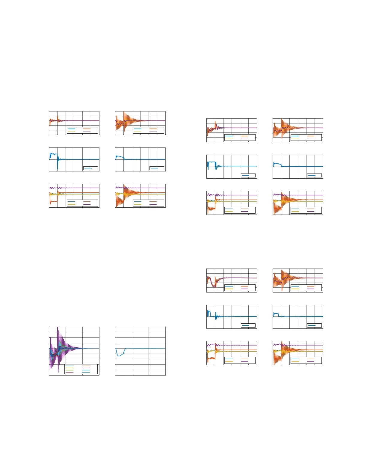
1 Frequenc y Stability Using MPC-based In v erter Po wer Control in Lo w-Inertia Po wer Systems Atinuke Ademola-Ido wu and Baosen Zhang Abstract —The electrical grid is ev olving from a netw ork consist- ing of mostly synchronous machines to a mixtur e of synchronous machines and in verter -based resources such as wind, solar , and energy storage. This transformation has led to a decrease in mechanical inertia, which necessitate a need for the new r esources to provide frequency responses through their inverter interfaces. In this paper we proposed a new strategy based on model predicti ve control to determine the optimal activ e-power set-point for inv erters in the event of a disturbance in the system. Our framework explicitly takes the hard constraints in power and energy into account, and we show that it is rob ust to measur ement noise, limited communications and delay by using an observer to estimate the model mismatches in real-time. W e demonstrate the proposed controller significantly outperf orms an optimally tuned virtual synchronous machine on a standard 39-bus system under a number of scenarios. In turn, this implies optimized in verter -based resources can provide better frequency responses compared to conv entional synchronous machines. I . I N T RO D U C T I O N The electric grid has been under going a transition from a network with dynamics fully gov erned by synchronous ma- chines to a mixed-source network with dynamics gov erned by both synchronous machines and in verter -based resources (IBRs). This transition is marked by a reduction in the amount of mechanical inertia in the system, which has led to more pronounced frequency responses to disturbances and faults in the grid [1], [2]. At the same time, by the virtue of the speed of power electronic circuits, IBRs such as solar, wind and energy storage have the capability to respond to frequency changes in the grid at a much faster rate than traditional generators with rotating masses. The challenge of how to best utilize these new capabilities has spurred much research interest in the last few years (e.g., see [3] and the references within). V arious control strategies that utilizes the IBRs in providing frequency regulation services has been proposed. The goal of these strategies is to design the activ e power response of the IBRs to changes in frequency , such that some frequency response objectiv e is minimized. For example, standard objec- tiv es of interests are the magnitude of the frequency deviation, the rate of change of frequency (R OCOF) and the settling The authors are with the Department of Electrical and Computer Engineer- ing at the University of W ashington, Seattle, W A 98195. Email: { aidowu, zhangbao } @uw .edu This work was partially supported by the National Science F oundation grant ECCS-1930605, the U.S. Department of Energys Office of Energy Efficienc y and Renewable Energy (EERE) under Solar Energy T echnologies Of fice (SETO) Agreement Number EE0009025 and the University of W ashington Clean Energy Institute. time. A unique challenge in the control of IBRs is that they tend to face much tighter limits than con ventional machines. For example, solar and wind resources cannot increase their power output beyond the maximum power tracking point, which introduces a hard (and asymmetrical) constraint on the action of the in verters. For a storage unit, it has only a limited amount of energy that can be used to respond to a disturbance. Of the v arying control strategies proposed for IBRs, Droop Contr ol [4]–[6] and V irtual Synchr onous Machines (VSMs) [7]–[9] are the most popular as they function by mimicking the frequency-po wer dynamic response of a synchronous machine. As suggested by their names, droop control injects/absorbs an amount of activ e power in proportion to the frequenc y deviation, and VSM, in its basic configuration, acts as a second order oscillator to provide inertia and damping to the grid. The parameters (droop slope, inertia and damping constants) used in these strategies can be optimized using a number of techniques [10]–[12]. The structural simplicity of VSMs also leads to a fundamental limitation [10], [15]. Since there are only two parameters to tune (inertia and damping) in the basic VSM configuration, there is an inherent trade-off between different objectiv es and there is no choice of parameters that will make the fre- quency deviation, R OCOF , and settling time small at the same time [10]. While the performance of the VSM can be enhanced by incorporating virtual governors, virtual exciters and other power systems controllers in their virtual form [13], [14], it difficult to tune the multiple parameters of the combined virtual controller simultaneously , since the performance of one might negati vely affect the other . In addition, it is also difficult to include hard constraints, since simply thresholding the output once the constraints are reached tend to lead to very poor performances [16]. Adapti ve rules can be used to alleviate this drawback somewhat, and works in [15], [17], [18] change the parameter based on the measured frequency deviation and R OCOF values. Howe ver , it is difficult to find an optimal rule to update these parameters in real-time. In this work, we propose a novel control strategy , based on model predicti ve control (MPC), called the MPC-based In verter Po wer Control (MIPC). W e explicitly formulate the problem of finding the optimal activ e power set-point of an IBR to minimize the frequency deviation and the ROCOF . It turns out that this formulation also implicitly minimizes the systems settling time. More specifically , at any timestep, we simulate the dynamics of the systems for a finite horizon, then find the best set-points that optimizes the objective ov er 2 that horizon. The first action is then adopted for the current timestep, and the process repeats. Our approach is similar in spirit to the ones in [15], [17], [18] since an objectiv e is optimized in an online fashion. Ho wever , instead of optimizing the parameters, we directly find the best po wer set-points. This approach turns out to provide both an easier optimiza- tion problem and better control performances. Namely , the hard constraints on the IBRs are explicitly included in the optimization process. A requirement of MPC is that the IBR must hav e a model of the system to be optimized. If wide-area measurements are av ailable, then the system states can be obtained from these measurements [19]. In some systems, only a limited buses are equipped with these measurement de vices (e.g. PMUs). W e show that our proposed MIPC frame work is still applicable to these systems by building an observer to estimate unmeasured disturbances and states. Through simulation studies, we show that the MIPC strictly outperforms optimally tuned VSMs for the IEEE 39-bus system, even under limited communication and large measurement noises. This proposed controller finds practical application by en- hancing the capability of the IBRs to participate in providing frequency regulation services. The additional power required can be obtained by running solar below its maximum power point to create suf ficient headroom, utilizing the inertia from the decoupled rotating wind turbine and, lev eraging on the stored energy in a battery . By explicitly considering hard constraints and costs on energy and po wer in the MPC formulation, economic considerations can be accounted for . The remainder of this paper is organized as follows: Section II defines the models used in this paper . Section III presents the design and formulation of the MIPC algorithm. Section IV presents the state and disturbance observer design. Section V compares the performances of MIPC to VSMs in a standard test system. Section VI concludes the paper . I I . M O D E L I N G W e denote the real line by R , the cardinality of a set S as |S | , the n × n identity and zero matrices as I n and 0 n , respectiv ely . Matrices and v ectors are denoted by a bold-faced variables. A. System Structur e Steady state conditions in a po wer systems are achie ved when there is a balance between the power produced by the generating sources and the power consumed by loads and lossy components. For stability analysis, the entire system can be reduced to an equi valent network via Kron reduction [20]. This eliminates passi ve and non-dynamic load buses and leav es only buses with at least one generating source connected. W ith this in place, frequency stability analysis can be carried out, with the frequency dynamics governed by the reactions of buses to activ e power imbalances in the system. In this work, we assume the a vailability of state variables and network information for control purposes. In a later section, we will relax this assumption to partial av ailability of state variables from some generators. Because the generators and IBRs had different dynamics, we denote their sets by G and I , respecti vely . Note that the total number of generating sources in the network is N : = G ∪ I . B. Synchr onous Machines The rotor dynamics of each synchronous generator in a giv en power system is governed by the well-known swing equation [21]. Here we adopt a discretized version of the equations, which in per unit (p.u.) system is: ω t +1 i = ω t i + h m i  P t m ,i − P t e ,i − d i ω t i  , δ t +1 i = ω b  δ t i + h ω t +1 i  , (1) ∀ i ∈ G where h is the step size for the discrete simulation, δ i (rad) is the rotor angle, ω = ¯ ω i − ω 0 is the rotor speed deviation, ω b is the base speed of the system, m i is the inertia constant, d i is the damping constant, P m ,i is the mechanical input power and P e ,i is the electric power output of the i th machine. The electrical output power P e ,i is giv en by the A C power flo w equation in terms of the internal emf | E i | and rotor angle δ i : P t e ,i = X i ∼ j | E i E j | [ g ij cos( δ t i − δ t j ) + b ij sin( δ t i − δ t j )] , (2) ∀ i, j ∈ G , where g ij + j b ij is the reduced admittance between nodes i and j . W e assume the internal emf are constant because of the actions of the exciter systems. The nonlinearity of the A C power flow in (2) makes (1) difficult to use for control applications. Linearizing (1) around the nominal point and using the DC power flow approximation [22], the b us dynamics become: 4 ω t +1 i = 4 ω t i + h m i  4 P t m ,i − 4 P t e ,i − d i 4 ω t i  , 4 δ t +1 i = ω b  4 δ t i + h 4 ω t +1 i  , (3) where 4 P t e ,i = P i ∼ j b ij 4 δ t ij is the dc power flo w between 2 buses. W e model changes to the mechanical input power 4 P t m ,i by a combination of droop and automatic governor control (A GC) actions [22]. C. V irtual Synchr onous Machine (VSM) From the network point of vie w , the grid-connected IBR is seen as producing a constant po wer according to its predeter- mined set-point and fast dynamics governed by closed-loop controls actions [23]. When configured in the grid-following mode, these controls help maintain the output power of the IBRs while remaining synchronized to the terminal voltage set by the grid [24]. For system analysis, the inv erter can be modeled as a v oltage source behind a reactance, much like a synchronous machine. 3 In the event of a power imbalance in the network reflected by a frequency deviation, an in verter does not hav e a ”natural” response to frequency de viation as synchronous machines does since they are made of power electronics components and ha ve no rotating mass. T o elicit some response, an additional control loop is therefore needed to enable the in verters to participate in frequency control by changing the power set-point of the in verter based on frequency measurements. The concept of virtual synchronous machine (VSM) has been proposed in literature to provide this additional control loop and it comes in different configurations [8], [25], [26]. The basic idea is to mimic the behavior of a synchronous machine’ s response to a frequency de viation by choosing appropriate gains cor- responding to the inertia and damping of the machines and producing power proportional to the R OCOF and frequency deviation. Since the response of the inv erter is entirely digital, it can be programmed with almost arbitrary functions. In this work, we adopt the VSM configuration in [26], where the additional power required to combat a frequency deviation is computed using: 4 P = 4 P km + 4 P kd = K m d 4 ω ibr dt + K d 4 ω ibr . (4) The local frequency at the IBR node 4 ω ibr is approximated by the center of inertia (COI) frequency [23], [27], which is an inertia-weighted a verage frequency giv en by: 4 ω ibr = P n i =1 m i 4 ω i P n i =1 m i (5) where n = |G | , 4 ω i is the rotor speed deviation, and m i is the inertia constant of the i th synchronous generators in the network. The gains K m and K d in (4) represent the virtual inertia and damping constants respectively . In contrast to synchronous machines where the constants are decided by the physical parameters, these constants of the VSM can be optimized over [10]. In the next section, we fully lev erage the flexibility of the power electronic interfaces using a MPC framew ork. I I I . M P C - BA S E D I N V E RT E R P O W E R C O N T RO L ( M I P C ) In this work, we propose a novel method for controlling the output po wer of the IBR, called the Inv erter Po wer Control (MIPC). This controller functions by modifying the initial real power set-point P 0 to a new set-point P ref as shown in Fig. 1 at each time step such that a weighted sum of the frequency deviation and ROCOF is minimized. Due to the timescale difference between IBRs and synchronous machines, the real power set-points of an IBR can be set almost instantaneously . Therefore, the important question becomes how to solve the optimization problem at each time step fast enough to find the real power set-point and how much communication is required in performing these calculations. In this section, we describe how to formulate the optimization problem and provide an efficient algorithm, assuming all of the information are known at the IBR. The next section then discusses how to deal with limited and noisy measurements, as well as incomplete communication. For the k th IBR, let u k denote its angle (referenced to the slack-bus). W e think of this u k as the control variable in the optimization problem. Note that the actual control of the IBR is not done via angle control, rather , we use the optimized u k to find the corresponding activ e po wer output of the in verter , then set the inv erter to that po wer . T o determine this real power set-point at a given time step, consider the po wer flow equation in (2), we write out the i th generator’ s power output P e ,i into two parts: power flowing from the i th generator to other generator denoted as P eG ,i and from the i th generator to IBRs denoted as P eI ,i , such that: P e ,i = P eG ,i + P eI ,i = X i ∼ j,i,j ∈G | E i E j | [ g ij cos( δ i − δ j ) + b ij sin( δ i − δ j )] + X i ∼ k,i, ∈G ,k ∈I | E i E k | [ g ik cos( δ i − u k ) + b ij sin( δ i − u k )] , (6) and the output power from the k th IBR denoted as P ibr ,k can also be written in two parts as: P ibr ,k = P ibr ,ki + P ibr ,kj , = X k ∼ i,k ∈I ,i ∈G | E k E i | [ g ki cos( u k − δ i ) + b ki sin( u k − δ i )] + X k ∼ j,j,k ∈I | E k E j | [ g kj cos( u k − u j ) + b kj sin( u k − u j )] . (7) A. Nonlinear Optimization Pr oblem At any timestep, we consider the behavior of the system N steps ahead. W ithout loss of generality , we start the problem at time t = 0 . The control variables are the inv erter angles, which we denote as u 0 , u 1 , . . . , u N − 1 . Once these are set, the rest of the system are gov erned by their swing equations. As stated before, the objectiv e is to minimize a function of the frequency deviation and the R OCOF , and the MIPC problem is giv en by: Min. { u 0 , u 1 ,..., u N − 1 } N − 1 X t =0  k ω t +1 k 2 2 + 1 h k ω t +1 − ω t k 2 2  (8a) s.t. ω t +1 i = ω t i + h m i  P t m ,i − P t e ,i − d i ω t i − 4 P t i  , ∀ i ∈ G (8b) P t e,i = Equation (6) , ∀ i ∈ G (8c) P t ibr,k = Equation (7) , ∀ k ∈ I (8d) P t ibr ,min ,k ≤ P t ibr ,k ≤ P t ibr ,max ,k , (8e) N X t =1 P t ibr ,k ≤ E t ibr , tot ,k , (8f) where ω t +1 ∈ R |G | is a v ector of all machine frequenc y deviations at the next time step and ω t +1 − ω t is a vector of all machine R OCOF between the current and next time step. The ev olution of ω is given in (8b) (swing equations) with the added 4 P i used to denote disturbances to the network which can be either a loss in generation or load, the power constraints are giv en in (8e) and the energy constraints are in (8f). Here we take the frequency deviation and the R OCOF to 4 be equally weighted for simplicity , but their weighting can be adjusted as needed for different practical scenarios. After (8) is solved, the control variable u 0 is substituted into the po wer flow equations (7) to find the acti ve power set-points of the IBRs. Then the IBRs hold their power at these set-points until the next time the optimization problem is solved. This is in line with the MPC conv ention, where the optimal control action is computed for the whole control horizon and only the first action is used. The process is then repeated again to determine the ne w control action. It turns out that the A C power flo w equations in (6) and (7) makes the problem nonlinear and dif ficult to solve in real-time. Therefore, the next two sections uses DC power flow to obtain an approximate problem that is much easier to solve. + + Inverter Operation P P ref P 0 P ibr Measurements Optimization Fig. 1. Block Diagram showing the operation of the MIPC controller which utilizes state and network variables to modify the real power set-point of the IBR at each timestep B. Unconstrained Linearized Pr oblem The main source of non-linearity in (8) comes from the A C po wer flo w equations in (8c) and (8d) and we use the standard DC power flow model from (3) to approximate these equations. Therefore, at b us i ∈ G (synchronous machines), we hav e: 4 P e,i = 4 P eG,i + 4 P eI ,i = X i ∼ j,j ∈G b ij ( 4 δ i − 4 δ j ) + X i ∼ j,k ∈I b ik ( 4 δ i − u k ) , (9) which can be written in matrix form as: 4 P e =  b ii − b ij − b j i b j j  | {z } B GG  4 δ i 4 δ j  +  − b ik − b j k  | {z } B GI u k , (10) where B GG contains the connection between synchronous generators and B GI contains the connection between a syn- chronous generator and IBRs. In state space form, it becomes  4 ω t +1 4 δ t +1  | {z } x t +1 =  − M − 1 D − M − 1 B GG I n 0 n  | {z } ¯ A  4 ω t 4 δ t  | {z } x t (11) +  − M − 1 B GI 0 n  | {z } ¯ B u u t +  − M − 1 0 n  | {z } ¯ B d 4 P t | {z } d t where 4 δ ∈ R n is the rotor angles deviation, 4 ω ∈ R n is the rotor speed de viation, M = diag ( m 1 , . . . , m n ) ∈ R n × n , D = diag ( d 1 , . . . , d n ) ∈ R n × n , 4 P t ∈ R n is vector of all power deviations which comes from the disturbances and noises in the system, denoted by d t . Since the MIPC does not kno w the disturbance or noise impacting the system, we use a two step process to solve the optimization problem. First, we ignore the disturbance term such that the MIPC’ s model of the system is:  4 ω t +1 4 δ t +1  | {z } x t +1 =  − M − 1 D − M − 1 B GG I n 0 n  | {z } ¯ A  4 ω t 4 δ t  | {z } x t (12) +  − M − 1 B GI 0 n  | {z } ¯ B u t . Note that in this case the MIPC’ s model of the system is actually wrong since the disturbances are not modeled. It turns out that this model is still useful, since the measurements are updated every time the MPC problem is solved, and this com- pensates for using a wrong model. In the rest of this section, we focus on solving the optimization problem using the model in (12) since it illustrates our methodology . Of course, when the measurement noise in the system is large or not every bus is equipped with wide-area measurement devices, it becomes necessary to explicitly estimate the mismatch between the model and the actual system. W e do so in section IV. W e reformulate the objective function in terms of the network model in (12) by defining the output of the linearized model as the frequenc y deviation 4 ω t : y t =  I n 0 n  | {z } C x t = 4 ω t (13) such that the R OCOF becomes: 4 y t = 1 h h y t − y t − 1 i = 1 h h 4 ω t − 4 ω t − 1 i (14) The MIPC optimization algorithm in (8) without the po wer limit constraint (8e) and total energy constraints (8f) can now be written as a linear quadratic programming problem: Min. u t J = 1 2 N − 1 X t =0 h y t T Q 1 y t + 4 y t T Q 2 4 y t i s.t. x t +1 = ¯ Ax t + ¯ B u t y t = C x t . (15) This can be written in matrix form for N time step ahead as: Min. u J = 1 2 x 0 T Gx 0 + x 0 T F u + 1 2 u T H u . (16) where H and F are constant matrices depending on ¯ A and ¯ B (see Appendix). C. Constrained Linearized Optimization Pr oblem In the presence of constraints, the problem becomes: Min. u J = 1 2 x 0 T Gx 0 + x 0 T F u + 1 2 u T H u s.t. Lu ≤ W + V x 0 , (17) where L , W and V encodes the constraints. In this paper , we consider constraints on the power output at each time step (8e) and constraints on the total energy av ailable (8f). This problem is a linearly constrained quadratic program and is con vex. 5 1) P ower Output Constraint: In practical considerations, there can be a limit on the amount of instantaneous power that can be drawn from the IBR due to factors such as the distance to the maximum power tracking operating point, the current ratings and switching speed of some power electronics components, and also power capability or C-rate of a battery . The transformation of the minimum and maximum instanta- neous power limit from P t ibr ,min ,k ≤ P t ibr ,k ≤ P t ibr ,max ,k to the linear constraint in (17) in volv es writing the linearized po wer output of the k th IBR at time step t in terms of the control variable u t and states x t , and then stacking them in matrix form for the N control horizon. The linearized output power P t ibr ,k is written in terms of the power flow to generators and to other IBRs as: P t ibr ,k = X k ∼ i,k ∈I ,i ∈G b ki ( u t k − 4 δ t i ) + X k ∼ j,j,k ∈I b kj ( u t k − u t j ) = − X k ∼ i,i ∈G b ki 4 δ t i + X k ∈I b kk u t k − X k ∼ j,j ∈I b kj u t j , which can be written in matrix form as: P t ibr ,k =  0 n − [ B ] ki  x t +  − [ B ] kj [ B ] kk  u t (18) Stacking (18) for a N time horizon and writing the linear system dynamics in term of the initial state results in a form: P ibr ,k = B p1 x 0 + B p2 u , (19) which can finally be written in the linear constraint form of (17) as  − B p2 B p2  | {z } L u ≤  − P ibr , min P ibr , max  | {z } W +  B p1 − B p1  | {z } V x 0 . (20) See appendix for deriv ation. 2) T otal Ener gy Constraint: This constraint occurs when there is a limit on the energy capacity of the IBR as in the case of a battery . For this constraint to be fully satisfied, the total energy not only at the end of the control horizon but also at each rolling sum of the consecuti ve time step should be less than the maximum energy capacity . As with the po wer output constraint, the total ener gy constraint P N t =1 P t ibr ,k ≤ E t ibr , tot ,k can also be written in the linear constraint form in (17) by taking the rolling sum ov er the in verter power output matrix in (19). This results in another matrix of the form: E ibr ,k = B e1 x 0 + B e2 u . (21) T o av oid a sudden decline in the power output when the maximum av ailable energy limit is reached, a rate constraint can be added to the power output decline between a specified consecutiv e time step. This can also be represent in the form of (17) by taking a one time step difference of the IBR power output matrix in (19), that is, a difference between the next time step and current time step IBR power output. This results in a matrix of the form: B r1 x 0 + B r2 u ≤ 4 P ibr ,k , . (22) Equation (21) and (22) can finally be written in the linear constraint form of (17) as  B e2 B r2  | {z } L u ≤  E ibr , tot   | {z } W +  − B e1 − B r1  | {z } V x 0 . (23) where  is a vector of IBR power output rate limit for each one time step difference. See appendix for deri vation. Even with constraints, a linear quadratic program can be solved extremely ef ficiently for systems with thousands of variables and constraints [28]. Again, to actually implement the controller , we compute and set the power output of the IBRs. I V . M I P C W I T H S TA T E E S T I M A T I O N A N D L I M I T E D C O M M U N I C A T I O N In section III, the MIPC controller was designed using the reduced linearized model of the network as in (12) and under the assumption of a full state measurement. When operating this controller in a realistic setting, we would want the controller to be robust against issues such as model mismatch, that is, the difference between the actual system model and the linearized model used by the MIPC; noisy measurements, and incomplete measurements because of limited communication between buses. W e address these issues in this section by integrating an observer into the MIPC controller system according to Fig. 2 to enable the controller estimate a better model of the system from the recei ved measurements. Power Systems Observer Controller y t ˆ x t K ( y t − ˆ y t ) MIPC P ibr ( u t ) Fig. 2. Observer inte grated MIPC in a power systems. The state measurements receiv ed by the observer in addition to the predicted state by the model is used to estimate the true state of the system. Let the dynamics of the actual power systems gov erned by (1) be represented concisely as: x t +1 = f ( x t , u t ) y t = g ( x t , u t ) . (24) A simple discrete observer model design [29] for the system in (24) can be written as: ˆ x t | t = ˆ x t | t − 1 + K ( y t − ˆ y t ) ˆ y t = C ˆ x t | t − 1 , (25) where the notation ˆ x t | τ means the prediction of x t made at time τ . Therefore the variables with ˆ x t | t is the updated observer state prediction based on new measurement y t , ˆ x t | t − 1 is the observer state prediction of the current time step using measurements from the previous time step, and K is a gain chosen such that the error between the measured and predicted state y t − ˆ y t is quickly dri ven to zero. 6 A. State and Disturbance Estimation T o estimate the state and disturbance in a noisy system with model mismatch and other forms of disturbance, we redefine d t as a vector of all disturbances. W e then integrate an input/output constant disturbance model [29] into the MIPC system model in (11) to obtain: ˆ x t +1 = ¯ A ˆ x t + ¯ B u u t + ¯ B d ˆ d t ˆ d t +1 = ˆ d t ˆ y t = C ˆ x t + C d ˆ d t , (26) where the disturbance ˆ d is modeled as a constant disturbance for the control period. Equation (26) can then be written in an augmented form as: " ˆ x t +1 ˆ d t +1 # =  ¯ A ¯ B d 0 I  " ˆ x t ˆ d t # +  ¯ B u 0  u t (27) ˆ y t =  C C d  " ˆ x t ˆ d t # . The predicted augmented state and disturbance can then be estimated using the observer model in (25) as: " ˆ x t | t ˆ d t | t # = " ˆ x t | t − 1 ˆ d t | t − 1 # + K   y t −  C C d  T " ˆ x t | t − 1 ˆ d t | t − 1 #   (28) where K is the gain matrix for the augmented state and disturbance v ariable. For simplicity , we adopt a fixed gain structure for the gain matrix K . This observer inte grated MIPC model in (27) and (28) replaces the linear model in (12), with the augmented state used in place of the original states x t and the rest of the algorithm follows through for the constrained and unconstrained case. B. Limited Communication While wide area measurement and communication systems are becoming increasingly av ailable [30], many networks still do not yet have real-time communication capabilities. Even for system with these types of infrastructure, there is always the possibility of communication issues. T o tackle the issue of limited communication, we assume that the initial state measurements of the generators is av ailable. For e xample, these can be con veyed using the existing SCAD A system ev ery two to four seconds. The augmented state and disturbance estimate in (28) is then used in estimating the full state and disturbance. The only difference is in the gain used since the structure and dimension of the gain K will change depending on the number of generators with a vailable state information, that is, the dimension of y t . The key idea here is that the mismatch between the e volv ed initial state of the generators with limited communication and what the state should be if there was communication is reflected as a disturbance in the network and can be estimated using the measurements from a vailable generators. V . C A S E S T U D I E S In this section, we validate the performance and versatility of the MIPC controller by testing it on the popular IEEE New England 10-machine 39-bus (NE39) system used for power systems dynamics stability studies [31]. W e study scenarios including constraints on the power and energy output of the IBR, noisy measurements and limited communication. Under each scenario, a large disturbance in the form of a partial generating capacity loss is applied to a generator in the network to initiate an event that can lead to a marked frequency decline. The performance metrics for the controller is its ability to maintain the frequency deviation within a small range, quickly recovering to the nominal frequency value and limiting the R OCOF . The network is transformed into a lo w-inertia netw ork by removing the interconnection to the rest of the US network and replacing generator 5 at bus 34 with an IBR whose total aggregated capacity equal to the replaced generator as sho wn in Fig. 3, and reduced to an equiv alent network using Kron reduction. The integrated IBR can be made up of either solar or wind but will be coupled with energy storage devices to guarantee the av ailability of the required capacity for frequency control. The step size for the discrete simulation is set to 0.05 (50ms) and the simulation starts of with the network in steady state, after which a disturbance of 60% loss of capacity is applied to the fourth generator ( G4 ) located at bus 33 from 0.5 to 5 seconds. G2 G1 G4 G3 G7 G6 G9 G8 1 2 3 4 5 6 7 8 9 10 11 12 13 14 15 16 17 18 19 20 21 22 23 24 25 26 27 28 29 30 31 32 33 34 35 36 37 38 Fig. 3. New England 39-bus system schematic with generator 5 at bus 34 replaced with an IBR of equal aggregated capacity . The performance of the proposed controller is compared to that of an optimally tuned VSM controller discussed in Section II-C with computed optimal gain coefficients of K m = 201 . 7 and K d = 520 according to [10]. Note that the VSM controllers simply saturates when it hits its power or energy limits. 7 1) Unconstrained Scenario: Fig. 4 sho ws the generator fre- quencies and IBR output power of the MIPC and VSM where there are not energy nor power limits. For a clearer viewing, only the frequency response of the second (slack), fourth (disturbed), sev enth and ninth generator are shown. The proposed MIPC controller keeps the frequencies within 0.2 Hz of nominal and restores the frequency to its nominal value, while under the VSM controller , the frequency varies by about 0.4 Hz and oscillates for a much longer time. 0 5 10 15 20 25 30 Time in seconds 59.4 59.6 59.8 60 60.2 60.4 Frequency in Hz frequency - MIPC Gen2 Gen4 Gen7 Gen9 0 5 10 15 20 25 30 Time in seconds 59.4 59.6 59.8 60 60.2 60.4 Frequency in Hz frequency - VSM Gen2 Gen4 Gen7 Gen9 0 5 10 15 20 25 30 Time in seconds 0 5 10 Power in pu inverter output power - MIPC Inv5 0 5 10 15 20 25 30 Time in seconds 0 5 10 Power in pu inverter output power - VSM Inv5 0 5 10 15 20 25 30 Time in seconds 0 5 10 Power in pu generator output power - MIPC Gen2 Gen4 Gen7 Gen9 0 5 10 15 20 25 30 Time in seconds 0 5 10 Power in pu generator output power - VSM Gen2 Gen4 Gen7 Gen9 Fig. 4. Comparison of MIPC and VSM control strategies for an unconstrained scenario in a NE39 network. The plots show the frequency and generator output power for some select generators and the IBR’ s output po wer . The MIPC outperforms the VSM in keeping the frequencies within limits. This sho ws the look-ahead and adapti ve nature of the pro- posed MIPC controller enables it outperform the VSM by utilizing the resources av ailable to satisfy the giv en objecti ve. It overcomes a particular issue of when the local frequency measurement becomes misleading a network with different coherent areas swinging against each other . Fig. 5 sho ws the center of inertia frequency gi ven by (5) when utilizing the VSM control structure compared to the true frequency of each generators, which the former is misleadingly small. 0 10 20 30 Time in seconds 59.5 59.6 59.7 59.8 59.9 60 60.1 60.2 60.3 60.4 frequency in Hz frequency deviation of generators Gen1 Gen2 Gen3 Gen4 Gen6 Gen7 Gen8 Gen9 0 10 20 30 Time in seconds 59.5 59.6 59.7 59.8 59.9 60 60.1 60.2 60.3 60.4 frequency in Hz center of inertia frequency Fig. 5. Frequencies of the individual generators (left) and the frequency of the center of inertia (right). 2) P ower and Ener gy Constraints: Figs. 6 and 7 sho ws select generators’ frequency and output po wer , and also the IBR output power for a po wer MIPC and VSM, respecti vely . The maximum po wer limits at each time step was set to 7 pu while the total energy limit was set to 70 pu. For a clearer viewing, only the frequency response of the second (slack), fourth (disturbed), seventh and ninth generator are shown. Compared to the VSM, the MIPC is still able to limit the frequency deviation to about 0.3 Hz for the limited po wer case and 0.4Hz for the limited energy case, while keeping the system frequency from rapid oscillation as seen in the VSM case. This expected since the MIPC is able to integrate the resource constraints into its optimization but is very hard to achiev ed using a VSM controller since it lacks an explicit optimization step to deal with hard constraints. Similar performances are observed in the ener gy-limited setting, which we do not show because of space constraints. 0 5 10 15 20 25 30 Time in seconds 59.4 59.6 59.8 60 60.2 60.4 Frequency in Hz frequency - MIPC Gen2 Gen4 Gen7 Gen9 0 5 10 15 20 25 30 Time in seconds 59.4 59.6 59.8 60 60.2 60.4 Frequency in Hz frequency - VSM Gen2 Gen4 Gen7 Gen9 0 5 10 15 20 25 30 Time in seconds 0 5 10 Power in pu inverter output power - MIPC Inv5 0 5 10 15 20 25 30 Time in seconds 0 5 10 Power in pu inverter output power - VSM Inv5 0 5 10 15 20 25 30 Time in seconds 0 5 10 Power in pu generator output power - MIPC Gen2 Gen4 Gen7 Gen9 0 5 10 15 20 25 30 Time in seconds 0 5 10 Power in pu generator output power - VSM Gen2 Gen4 Gen7 Gen9 Fig. 6. Comparison of MIPC and VSM control strategies for a po wer constrained scenario in a NE39 network. The MIPC controller is able to adaptiv ely change its power output to minimize frequency de viations while respecting the power limits 0 5 10 15 20 25 30 Time in seconds 59.4 59.6 59.8 60 60.2 60.4 Frequency in Hz frequency - MIPC Gen2 Gen4 Gen7 Gen9 0 5 10 15 20 25 30 Time in seconds 59.4 59.6 59.8 60 60.2 60.4 Frequency in Hz frequency - VSM Gen2 Gen4 Gen7 Gen9 0 5 10 15 20 25 30 Time in seconds 0 5 10 Power in pu inverter output power - MIPC Inv5 0 5 10 15 20 25 30 Time in seconds 0 5 10 Power in pu inverter output power - VSM Inv5 0 5 10 15 20 25 30 Time in seconds 0 5 10 Power in pu generator output power - MIPC Gen2 Gen4 Gen7 Gen9 0 5 10 15 20 25 30 Time in seconds 0 5 10 Power in pu generator output power - VSM Gen2 Gen4 Gen7 Gen9 Fig. 7. Comparison of MIPC and VSM control strategies for an energy constrained scenario in a NE39 network. The MIPC controller is also able to adaptiv ely change its power output to ensure that the energy limits over its operation horizon are respected. 3) Robustness of the Contr oller: Fig. 8 demonstrates the robustness of the MIPC controller to noise, model mismatch and external disturbances to the system with the incorporation of the observer model in (28). W e model noisy measurements by adding Gaussian noise to create SNRs of 30dB and 50dB, respectiv ely representing the worst-case and an average-case 8 SNR scenarios [32], [33]. Fig. 8 shows that noise has very little impact to the performance of the MIPC (even under 30 dB of SNR). Of course, the observer plays an important role in this rob ustness to noisy measurements. 0 10 20 30 Time in seconds 59.7 59.8 59.9 60 60.1 60.2 Frequency in Hz frequency - MIPC with 30dB noise Gen2 Gen4 Gen7 Gen9 0 10 20 30 Time in seconds 59.7 59.8 59.9 60 60.1 60.2 Frequency in Hz frequency - MIPC with 50dB noise Gen2 Gen4 Gen7 Gen9 0 10 20 30 Time in seconds 0 2 4 6 8 Power in pu inverter output power - MIPC with 30dB noise Inv5 0 10 20 30 Time in seconds 0 2 4 6 8 Power in pu inverter output power - MIPC with 50dB noise Inv5 Fig. 8. Comparison of robust MIPC under SNR of 30dB and 50dB. The MIPC controller is still able achiev e a smooth response while keeping the frequency within limit even in a worst-case noise scenario. 4) Limited Communication: W e further test the performance of the MIPC in a limited communication scenario. In the partial communication scenario, we assume that measurements can be receiv ed from the generators G3, G4, G6, and G7 while only initial state measurements is receiv ed from the generators G1, G2, G8 and G9 in Fig. 3 (so faulted generator (G4) is able to communicate with the inv erter). The left-side plot of Fig. 9 sho ws the MIPCs performance under the partial communication scenario. By communicating with some buses, the MIPC is able to reconstruct enough of the system-level information to make the computations at the MIPC useful. The right-side plot of Fig. 9 shows the no-communication sce- nario, where none of the generators can exchange information with each other . Here the MIPC performs much like a VSM. This is expected since without communication, the best MIPC can do is to utilize its local measurements to take actions. 0 10 20 30 Time in seconds 59.6 59.8 60 60.2 60.4 Frequency in Hz frequency - MIPC partial communication Gen2 Gen4 Gen7 Gen9 0 10 20 30 Time in seconds 59.6 59.8 60 60.2 60.4 Frequency in Hz frequency - MIPC no communication Gen2 Gen4 Gen7 Gen9 0 10 20 30 Time in seconds 0 2 4 6 8 Power in pu inverter output power - MIPC partial communication Inv5 0 10 20 30 Time in seconds 0 2 4 6 8 Power in pu inverter output power - MIPC no communication Inv5 Fig. 9. MIPC control actions under a partial and no-communication scenario. 5) Delayed Communication: In the previous scenarios, we assumed that the measurements are receiv ed in time for the controller to perform its computations. In this delayed communication scenario, we assume that there is a delay in measurement data received from some generators in the network. Fig. 10 shows the MIPC performance when a delay in measurement receiv ed is applied at random to any four generators thus creating a possibility for the controller to receiv e delayed measurements from the faulted generator (G4). The left-side plot of Fig. 10 shows a one time step delay , that is, a delay of 50ms, while the right-side plot shows a three time step delay , that is, a delay of 150ms. It can be observed that the MIPC controller is still able to determine the appropriate in verter set-point to drive the system to stability albeit with deteriorating performance as the time lag increases. 0 10 20 30 Time in seconds 59.6 59.8 60 60.2 60.4 Frequency in Hz frequency - MIPC one timestep delay Gen2 Gen4 Gen7 Gen9 0 10 20 30 Time in seconds 59.6 59.8 60 60.2 60.4 Frequency in Hz frequency - MIPC three timestep delay Gen2 Gen4 Gen7 Gen9 0 10 20 30 Time in seconds 2 3 4 5 6 7 8 Power in pu inverter output power - MIPC one timestep delay Inv5 0 10 20 30 Time in seconds 2 3 4 5 6 7 8 Power in pu inverter output power - MIPC three timestep delay Inv5 Fig. 10. MIPC control actions under a one- and three- time step delayed communication scenario. V I . C O N C L U S I O N In this paper , we proposed a nov el control strategy called the In verter Power Control that optimally determines the acti ve power set-point for an in verter -based resource in real-time. Using a model predicti ve control framework, hard po wer and energy constraints are considered explicitly in the optimiza- tion process. W e show via simulation on a test system the superiority of the proposed controller in comparison to the optimally tuned virtual synchronous machine, under both noisy and limited communication settings. Our future work explores enhancing the controller to function in a large network with multiple IBRs, integrating model identification techniques and robustness to communication delays. R E F E R E N C E S [1] J. Machowski, J. Bialek, and J. Bumby , P ower system dynamics: stability and contr ol . John Wile y & Sons, 2011. [2] P . T ielens and D. V an Hertem, “The relev ance of inertia in power systems, ” Renewable and Sustainable Energy Reviews , vol. 55, pp. 999– 1009, 2016. [3] F . Milano, F . D ¨ orfler , G. Hug, D. J. Hill, and G. V erbi ˇ c, “Foundations and challenges of low-inertia systems, ” in 2018 P ower Systems Computation Confer ence (PSCC) . IEEE, 2018, pp. 1–25. 9 [4] J. V an de Vyver , J. D. De K ooning, B. Meersman, L. V andevelde, and T . L. V andoorn, “Droop control as an alternativ e inertial response strategy for the synthetic inertia on wind turbines, ” IEEE T ransactions on P ower Systems , vol. 31, no. 2, pp. 1129–1138, 2015. [5] J. W . Simpson-Porco, F . D ¨ orfler , and F . Bullo, “Synchronization and power sharing for droop-controlled in verters in islanded microgrids, ” Automatica , vol. 49, no. 9, pp. 2603–2611, 2013. [6] R. Ofir, U. Markovic, P . Aristidou, and G. Hug, “Droop vs. virtual inertia: Comparison from the perspective of con verter operation mode, ” in 2018 IEEE International Ener gy Confer ence (ENERGYCON) . IEEE, 2018. [7] M. V an W esenbeeck, S. De Haan, P . V arela, and K. V isscher, “Grid tied con verter with virtual kinetic storage, ” in P owerT ech, 2009 IEEE Buchar est . IEEE, 2009, pp. 1–7. [8] K. Sakimoto, Y . Miura, and T . Ise, “Stabilization of a po wer system with a distributed generator by a virtual synchronous generator function, ” in P ower Electronics and ECCE Asia (ICPE & ECCE), 2011 IEEE 8th International Conference on . IEEE, 2011, pp. 1498–1505. [9] Q.-C. Zhong and G. W eiss, “Synchron verters: Inv erters that mimic synchronous generators, ” IEEE T ransactions on Industrial Electronics , vol. 58, no. 4, pp. 1259–1267, 2011. [10] A. Ademola-Idowu and B. Zhang, “Optimal design of virtual inertia and damping coefficients for virtual synchronous machines, ” in P ower and Ener gy Society General Meeting , 2018. [11] T . Borsche and F . D ¨ orfler , “On placement of synthetic inertia with explicit time-domain constraints, ” arXiv pr eprint arXiv:1705.03244 , 2017. [12] B. K. Poolla, S. Bolognani, and F . Dorfler, “Optimal placement of virtual inertia in power grids, ” IEEE Tr ansactions on Automatic Contr ol , 2017. [13] Y . Hirase, K. Abe, K. Sugimoto, and Y . Shindo, “ A grid-connected in verter with virtual synchronous generator model of algebraic type, ” Electrical Engineering in Japan , vol. 184, no. 4, pp. 10–21, 2013. [14] G. Y ao, Z. Lu, Y . W ang, M. Benbouzid, and L. Moreau, “ A virtual synchronous generator based hierarchical control scheme of distributed generation systems, ” Ener gies , vol. 10, no. 12, p. 2049, 2017. [15] F . W ang, L. Zhang, X. Feng, and H. Guo, “ An adaptiv e control strategy for virtual synchronous generator , ” IEEE T ransactions on Industry Applications , vol. 54, no. 5, pp. 5124–5133, 2018. [16] M. Polycarpou, J. Farrell, and M. Sharma, “On-line approximation con- trol of uncertain nonlinear systems: issues with control input saturation, ” in Pr oceedings of the 2003 American Contr ol Conference, 2003. , vol. 1. IEEE, 2003, pp. 543–548. [17] D. Li, Q. Zhu, S. Lin, and X. Bian, “ A self-adaptiv e inertia and damping combination control of vsg to support frequency stability , ” IEEE T ransactions on Ener gy Conver sion , vol. 32, no. 1, pp. 397–398, 2017. [18] C. Zhang, Y . Y ang, H. Miao, and X. Y uan, “ An improved adapti ve inertia and damping control strategy for virtual synchronous generator, ” in 2018 13th IEEE Conference on Industrial Electr onics and Applications (ICIEA) . IEEE, 2018, pp. 322–328. [19] F . D ¨ orfler , M. R. Jovano vi ´ c, M. Chertkov , and F . Bullo, “Sparsity- promoting optimal wide-area control of power networks, ” IEEE T rans- actions on P ower Systems , vol. 29, no. 5, pp. 2281–2291, 2014. [20] T . Nishikawa and A. E. Motter , “Comparativ e analysis of existing mod- els for power -grid synchronization, ” New Journal of Physics , vol. 17, no. 1, p. 015012, 2015. [21] P . W . Sauer, M. Pai, and J. H. Chow , P ower system dynamics and stability: with synchr ophasor measurement and power system toolbox . John Wile y & Sons, 2017. [22] P . Kundur , “Power system control and stability , ” New Y ork: McGraw , 1994. [23] H. N. V . Pico and B. B. Johnson, “Transient stability assessment of multi-machine multi-conv erter power systems, ” IEEE T ransactions on P ower Systems , 2019. [24] J. Rocabert, A. Luna, F . Blaabjerg, and P . Rodriguez, “Control of power con verters in ac microgrids, ” IEEE transactions on power electr onics , vol. 27, no. 11, pp. 4734–4749, 2012. [25] J. Alipoor, Y . Miura, and T . Ise, “Power system stabilization using virtual synchronous generator with alternating moment of inertia, ” IEEE Journal of Emer ging and Selected T opics in P ower Electr onics , vol. 3, no. 2, pp. 451–458, 2015. [26] H. Bevrani, T . Ise, and Y . Miura, “V irtual synchronous generators: A survey and new perspectives, ” International Journal of Electrical P ower & Energy Systems , vol. 54, pp. 244–254, 2014. [27] B. J. Pierre, H. N. V illegas Pico, R. T . Elliott, J. Flicker, Y . Lin, B. B. Johnson, J. H. Eto, R. H. Lasseter, and A. Ellis, “Bulk power system dynamics with varying levels of synchronous generators and grid-forming power in verters, ” National Renewable Ener gy Lab .(NREL), Golden, CO (United States), T ech. Rep., 2019. [28] J. Nocedal and S. Wright, Numerical optimization . Springer Science & Business Media, 2006. [29] G. Pannocchia and J. B. Rawlings, “Disturbance models for offset-free model-predictiv e control, ” AIChE journal , vol. 49, no. 2, pp. 426–437, 2003. [30] A. G. Phadke and B. T ianshu, “Phasor measurement units, wams, and their applications in protection and control of power systems, ” Journal of Modern P ower Systems and Clean Energy , vol. 6, no. 4, pp. 619–629, 2018. [31] R. Ramos, I. Hiskens et al. , “Benchmark systems for small-signal stability analysis and control, ” IEEE P ower and Energy Society , 2015. [32] “Ieee/iec international standard - measuring relays and protection equip- ment - part 118-1: Synchrophasor for power systems - measurements, ” IEC/IEEE 60255-118-1:2018 , pp. 1–78, Dec 2018. [33] R. Ghiga, K. Martin, Q. W u, and A. H. Nielsen, “Phasor measurement unit test under interference conditions, ” IEEE Tr ansactions on P ower Delivery , vol. 33, no. 2, pp. 630–639, 2017. A P P E N D I X C O N S T A N T G A I N M A T R I X F O R M I P C The matrices H and F in III-B can be obtained as follows: writing the linear system model in (12) for N time steps ahead in matrix form, we have:         x 0 x 1 x 2 . . . x N         | {z } x =         0 0 . . . 0 ¯ B 0 . . . 0 ¯ A ¯ B ¯ B . . . 0 . . . . . . . . . . . . ¯ A N − 1 ¯ B ¯ A N − 2 ¯ B . . . ¯ B         | {z } S       u 0 u 1 . . . u N − 1       | {z } u +         I ¯ A ¯ A 2 . . . ¯ A N         | {z } M x 0 (29) The objective function in (15) can then be written in terms of the state v ariable as: y T Q 1 y = ( C x ) T Q 1 ( C x ) = x T C T Q 1 C | {z } ˆ Q 1 x (30) =         x 0 x 1 x 2 . . . x N                 ˆ Q 1 0 0 . . . 0 0 ˆ Q 1 0 . . . 0 0 0 ˆ Q 1 . . . 0 . . . . . . . . . . . . 0 0 0 . . . ˆ Q 1         | {z } ˜ Q 1         x 0 x 1 x 2 . . . x N         = ( S u + M x 0 ) T ˜ Q 1 ( S u + M x 0 ) (31) 10 Let Θ = S [0 : N − 1; 1 : N ] − S [1 : N ; 1 : N ] (32) Γ = M [0 : N − 1] − M [1 : N ] 4 x = x [0 : N − 1] − x [1 : N ] such that 4 y T Q 2 4 y = ( C 4 x ) T Q 2 ( C 4 x ) (33) = 4 x T C T Q 2 C | {z } ˆ Q 2 4 x = (Θ u + Γ x 0 ) T ˜ Q 2 (Θ u + Γ x 0 ) Therefore (15) becomes: J = 1 2  ( S u + M x 0 ) T ˜ Q 1 ( S u + M x 0 ) + (Θ u + Γ x 0 ) T ˜ Q 2 (Θ u + Γ x 0 )  = 1 2 x 0 T h M T ˜ Q 1 M + Γ T ˜ Q 2 Γ | {z } G i x 0 + 1 2 u T h S T ˜ Q 1 S + Θ T ˜ Q 2 Θ | {z } H i u + x 0 T h M T ˜ Q 1 S + Γ T ˜ Q 2 Θ | {z } F i u J = 1 2 x 0 T Gx 0 + 1 2 u T H u + x 0 T F u (34) For optimality , ∇ J u = H u + F x 0 = 0 , such that the optimal control action at a giv en start point for N time horizon ahead becomes: u ∗ = − H − 1 F T x 0 . (35) P OW E R L I M I T The linear constraint equation for the IBR po wer limit in (20) can be deri ved by stacking (18) for a N step control horizon as follows:       P 1 ibr ,k P 2 ibr ,k . . . P N ibr ,k       | {z } P ibr ,k =       B p 1 0 . . . 0 B p 1 B p 1 . . . 0 . . . . . . . . . . . . B p 1 B p 1 . . . B p 1       | {z } B p 1 ,N       ˆ z 1 ˆ z 2 . . . ˆ z N       | {z } ˆ z +       B p 2 0 . . . 0 B p 2 B p 2 . . . 0 . . . . . . . . . . . . B p 2 B p 2 . . . B p 2       | {z } B p 2 ,N       u 0 u 1 . . . u N − 1       | {z } u . (36) From (29), we hav e that ˆ z = S u + M ˆ z 0 , therefore (36) becomes, P ibr ,k = B p 1 ,N S u + B p 1 ,N M ˆ z 0 + B p 2 ,N u = ( B p 1 ,N S + B p 2 ,N | {z } ˜ B p 1 ) u + B p 1 ,N M | {z } ˜ B p 2 ˆ z 0 . (37) The lower power limit can then be written as − ˜ B p 1 u ≤ − ˜ P ibr , min + ˜ B p 2 ˆ z 0 (38) and the upper power limit as ˜ B p 1 u ≤ ˜ P ibr , min − ˜ B p 2 ˆ z 0 (39) resulting in a combined form of: " − ˜ B p2 ˜ B p2 # | {z } L u ≤ " − ˜ P ibr , min ˜ P ibr , max # | {z } W + " ˜ B p1 − ˜ B p1 # | {z } V ˆ z 0 . (40) where ˜ P ibr , min and ˜ P ibr , max are matrices of ˜ P t ibr , min and ˜ P t ibr , max stacked together for N horizon. T OTA L E N E R G Y L I M I T The linear constraint equation for the IBR total energy limit in (23) can be derived from the po wer limit in (37) by taking the rolling sum such that: [ ˜ B p1 u + ˜ B p2 ˆ z 0 ] T 1 N ≤ ˜ E ibr , tot (41) resulting in 1 T N ˜ B p1 | {z } ˜ B e1 u ≤ ˜ E ibr , tot − 1 T N ˜ B p2 | {z } ˜ B e2 ˆ z 0 . (42) The rate limit, represented as  in this work, can be incorpo- rated by taking the difference between time steps of the output power in (37) such that: [ ˜ B p1 u + ˜ B p2 ˆ z 0 ] [1 : N − 1] − [ ˜ B p1 u + ˜ B p2 ˆ z 0 ] [2 : N ] (43) resulting in ˜ B p1 u + ˜ B p2 ˆ z 0 ] [1 : N − 1] − [ ˜ B p1 u + ˜ B p2 ˆ z 0 ] [2 : N ] (44) The combined form of these two constraints is: " ˜ B e2 ˜ B r2 # | {z } L u ≤ " ˜ E ibr , tot  # | {z } W + " − ˜ B e1 − ˜ B r1 # | {z } V ˆ z 0 . (45)