On Scaling Data-Driven Loop Invariant Inference

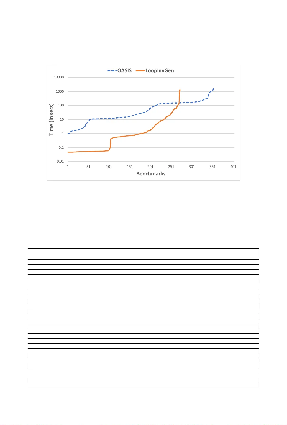
On Scaling Data-Driven Loop Invariant Inference SAHIL BHA TIA, Microsoft Research, India SASW A T P ADHI, University of California Los Angeles, USA NA GARAJAN NA T ARAJAN, Microsoft Research, India RAH UL SHARMA, Microsoft Research, India PRA TEEK JAIN, Microsoft Research, India A utomated synthesis of inductive invariants is an important problem in software verication. Once all the invariants have been sp ecied, software verication reduces to che cking of verication conditions. Although static analyses to infer invariants have been studied for over forty years, recent years have se en a urry of data-driven invariant inference techniques which guess invariants from examples instead of analyzing program text. How ever , these techniques have been demonstrated to scale only to programs with a small number of variables. In this paper , we study these scalability issues and address them in our tool Oasis that improves the scale of data-driven invariant inference and outperforms state-of-the-art systems on benchmarks from the invariant inference track of the Syntax Guided Synthesis competition. 1 INTRODUCTION Inferring inductive invariants is one of the core problems of softwar e verication. Recently , there has been a urr y of data-driven invariant inference techniques [Alur et al . 2017; Garg et al . 2014, 2016; Li et al . 2017; Nguyen et al . 2017, 2012; Padhi et al . 2016; Sharma and Aiken 2016; Sharma et al . 2013b,a, 2012; Thakur et al . 2015; Zhu et al . 2018] that learn invariants from examples. These data-driven techniques oer attractive features such as the ability to systematically generate disjunctive invariants. Whereas the well-know static invariant infer ence techniques either fail to infer disjunctive invariants [Colón et al . 2003; Cousot and Cousot 1977; Cousot and Halbwachs 1978; Miné 2006] or require a user-pr ovided bound on the number of disjunctions [Bagnara et al . 2006; Gulwani and Jojic 2007; Gulwani et al . 2008; Gupta et al . 2013; Sankaranarayanan et al . 2006]. At the heart of the data-driven techniques is an active learning [Hanneke 2009] loop: a learner guesses a candidate invariant fr om data and provides the candidate to a teacher . The teacher either validates that the candidate is a valid invariant or r eturns a counterexample. This example is added to the data and the process is repeated until the learner guesses a correct invariant. In this architecture, the more the numb er of program variables in the verication problem, the more the learner is likely to choose an incorrect candidate or take a long time to generate good candidates [Padhi et al . 2019]. Hence, as we discuss in our evaluation in Section 6, existing data-driven invariant inference techniques have been shown to be ee ctive only for programs with a small number of variables. For data-driven invariant inference to b e applicable to verication of practical softwar e, these scalability challenges must be addressed. There are two main obstacles to scalability which are related to the number of program variables: First, a pr ogram can hav e many variables and often only a small subset of these variables are rele vant to the invariants. Intuitively , writing corr ect programs that require complicated invariants with many variables is hard for developers and prior works on invariant inference are also biased towar ds simple invariants [Albarghouthi and McMillan 2013]. In the absence of a technique that separates the relevant variables from the irrelevant, the learner can get b ogged down by the irrelevant variables. In particular , invariant inference benchmarks in the Syntax Guided Synthesis (SyGuS) competition are pro vided as logic formulas where static slicing [Horwitz et al . 1988] fails to remo ve the semantically irr elevant variables. Second, data-driven A uthors’ addresses: Sahil Bhatia, Microsoft Research, India, t- sab@microsoft.com; Saswat Padhi, University of California Los Angeles, USA, padhi@cs.ucla.edu; Nagarajan Natarajan, Microsoft Research, India, nagarajn@micr osoft.com; Rahul Sharma, Microsoft Research, India, rahsha@microsoft.com; Prateek Jain, Microsoft Research, India, prajain@microsoft.com. 2 Sahil Bhatia, Saswat Padhi, Nagarajan Natarajan, Rahul Sharma, and Prateek Jain techniques also rely on some form of enumeration to generate candidate predicates. Thus, a higher number of variables causes the enumerator to take a long time to reach pertinent candidates. For example, if the enumerator exhaustiv ely generates expressions in increasing size [Alur et al . 2017; Padhi et al . 2019] then before enumerating expressions of size s , it must enumerate all expression of size s − 1 ov er all variables. T o exemplify these scalability issues, we consider LoopInvGen [Padhi et al . 2019, 2016], the state-of-the-art data-driven invariant infer ence tool that won in the invariant infer ence track of SyGuS competition held in 2017 and 2018. It uses exhaustive enumeration to synthesize Bo olean features (simple predicates). Then, a Boolean function learner generates a candidate invariant which is a Boolean combination of the features. As the numb er of program variables increases, the scalability degrades because the enumerator must explore exponentially many features and the learner needs many examples to avoid generating candidates with irrelevant variables; with a large number of variables, the learner can overt on the irrelevant variables to generate incorrect candidates that will be rejected by the teacher [Padhi et al. 2019]. W e explore addressing both the scalability issues, cause d by enumeration and irrele vant variables, through machine learning (ML). In particular , we make the following tw o contributions. First, we describe a learner that can infer the relevant variables, thus ensuring that data-driven invariant inference is only applied to the simpler problem with a few or no irrelevant variables. Since the number of relevant variables is typically small, data-driven invariant inference can scale to such tasks better . Second, we show that exhaustive enumeration can b e replaced by learners that are much more scalable. Instead of a generate-and-check approach where an enumerator generates all possible candidate features eagerly [Albarghouthi et al . 2013; Ernst et al . 2000; Padhi et al . 2016], w e employ a more scalable guess-and-check approach where the learner intelligently guesses features from data. W e have implemente d these techniques in a to ol Oasis 1 that takes as input logic formulas which encode the verication of safety properties of programs over integer variables and outputs inductive invariants that are sucient to prove the properties. T o this end, Oasis employs new ML algorithms for the well-known binary classication problem: the learner’s goal is to nd a classier that separates positive and negative examples. The classier is a predicate that includes the positive examples and excludes the negative examples. In the conte xt of invariant inference, an example is a program state that maps variables to integers. Oasis makes the following contributions. First, Oasis uses binar y classication to infer relevant and irr elevant variables (Section 4.3). It uses symbolic execution to generate reachable states (positive examples) and bad states (negative examples), which are backward reachable from states that violate the safety properties. Then it nds a sparse classier and we classify the variables occurring in the classier as relevant. If a variable is absent from the classier and it is possible to separate samples of reachable states from bad states without using the variable then it is likely to be irrelevant to the invariant. The sparsity requirement ensures that we keep the number of relevant variables to minimal. W e remark that we need a custom learner for this task. Each state (reachable or bad) is a partial map from variables to integers. In particular , there are some variables that are not in the domain of the state. These variables are don’t care , i.e. , they can be assigned any value without aecting the label (positive or negativ e) of the state. The (partial) models generated by SMT solvers typically have don’t cares. The well-known ML classiers learn over total maps as opposed to partial maps. Although one can extend a partial map to a total map by setting the don’t care variables to zero or randomly assigned values, these alternatives ar e undesirable as a partial map corresponds to an innite number of p ossible total maps and supplanting it with any total map loses the information 1 The name Oasis stands for O ptimization A nd S earch for I nvariant S ynthesis. On Scaling Data-Driven Loop Invariant Inference 3 encoded in the partial map. Hence, we hav e designed a custom learner that directly learns a classier using partial maps and is not limited to total maps. After we obtain the set of relevant variables from the classier , Oasis calls a modied version of LoopInvGen where the synthesis of features is restricted to predicates over the rele vant variables. Second, Oasis uses a learner to synthesize Boolean features from data (Section 4.4). Internally , LoopInvGen breaks do wn the problem of invariant inference into many small binary classication tasks and uses Escher [Albarghouthi et al . 2013] to nd features that solve them. Specically , Escher exhaustively enumerates all featur es in increasing size till it nds one that separates the positive examples from the negative examples in the small task. Oasis replaces Escher with a learner to nd such features. Unlike traditional ML algorithms that have non-zero error , i.e. , they fail to separate some positive examples from some negativ e examples, LoopInvGen requires the feature synthesizer to have zero error . Oasis uses the same learner to solve both these problems, i.e. , inferring relevant variables and inferring features. In particular , the learner of Oasis solves a non-standard ML problem: nding sparse classiers with zero error in the presence of don’t car es. W e describe a nov el learner that solves this problem (Section 5). T o the best of our knowledge, all prior works on data-driven invariant inference use learners that r equire total maps. W e show how to encode the problem of nding such a classier as an instance of integer linear programming (ILP) which minimizes an objective function subject to linear constraints. Although linear programming has previously been used to assist invariant inference [Gupta et al . 2013], our encoding is novel. Specically , we show how to systematically encode domain-specic heuristics as objective functions or constraints for eective learning in the context of invariant inference. Heavily optimized ILP solvers are available as o-the-shelf tools and Oasis uses them to scale data-driven invariant infer ence. T o demonstrate the scalability of Oasis in practice, we evaluate Oasis on over 400 benchmarks from the invariant (Inv) track of the Sy GuS competion held in 2019 [syg 5 14] (Section 6). This benchmark set includes the new community provided programs that have a large number of irrelevant variables which test the scalability of invariant synthesis tools [Si et al . 2018]. Our evaluation shows that Oasis signicantly improves the scalability of data-driven invariant inference on these b enchmarks and solves 20% more benchmarks than LoopInvGen , the state-of-the-art data- driven invariant inference tool. Oasis even outperforms state-of-the-art invariant inference tools that are based on very dierent techniques. It solves more benchmarks than de ductive synthesis implemented in CVC4 [Barrett et al . 2011; Reynolds et al . 2015] and cooperative synthesis of the recent work of Dry adSynth [Huang et al . 2020] that combines enumerative and deductive synthesis. Thus, our evaluation shows that Oasis signicantly improves the state-of-the-art in data-driven invariant inference and makes it as scalable as deductive and cooperative techniques. Oasis solves more benchmarks than these tools and also solves benchmarks that are beyond the reach of prior work. The rest of the paper is organized as follo ws. W e provide an e xample to show the end-to-end working of Oasis (Se ction 2) and review the relevant backgr ound (Section 3). W e describe Oasis in detail (Section 4) followed by the ILP-based learner (Section 5). W e evaluate Oasis in Se ction 6, place it in the context of the landscape of invariant inference techniques in Section 7, and conclude with directions for future work in Section 8. 4 Sahil Bhatia, Saswat Padhi, Nagarajan Natarajan, Rahul Sharma, and Prateek Jain 1: assume ( k ≥ 0 ∧ n ≥ 0 ) 2: i = j = 0 3: while ( i ≤ n ) do 4: ( i , j , y ) ← ( i + 1 , j + 1 , i × j ) 5: assert ( i + j + k ≥ 2 n ∨ y ≥ n 2 ) Fig. 1. The C-program of working e xample. 2 W ORKING EXAMPLE W e use a simple (contrived) benchmark to show the working of each comp onent of Oasis . The goal is to synthesize an inductive invariant I ( ® x ) , where ® x = ⟨ i , j , k , n , y ⟩ that satises the following verication conditions (V Cs) expressed as Horn Clauses. Pre ( ® x ) ⇒ I ( ® x ) with Pre ( ® x ) ≜ i = j = 0 ∧ k ≥ 0 ∧ n ≥ 0 I ( ® x ) ∧ Trans ( ® x , ® x ′ ) ⇒ I ( ® x ′ ) with Trans ( ® x , ® x ′ ) ≜ i ≤ n ∧ i ′ = i + 1 ∧ j ′ = j + 1 ∧ y ′ = i × j I ( ® x ) ⇒ Post ( ® x ) with Post ( ® x ) ≜ i ≤ n ∨ i + j + k ≥ 2 n ∨ y ≥ n 2 These V Cs encode the verication of the C-program in Figure 1. If there exists a predicate I that satisifes the VCs then for all possible inputs the assertion can never be violate d. A state for this example is a 5-tuple that maps i , j , k , n , y to integers or don’t cares (denoted by ⊤ ). The rst step is the identication of irrelevant variables. Oasis generates reachable states, i.e., p ositive examples by computing satisfying assignments of Pre ( ® x ) and Pre ( ® x ) ∧ Trans ( ® x , ® x ′ ) . For bad states, i.e., negative examples, Oasis computes satisfying assignments of ¬ Post ( ® x ) and ¬ Post ( ® x ′ ) ∧ Trans ( ® x , ® x ′ ) . These satisfying assignments are obtaine d from o-the-shelf SMT solvers and result in T able 1. i j k n y ℓ 0 0 0 0 ⊤ 1 2 3 0 1 2 1 1 -1 0 0 -1 0 6 4 0 5 15 0 T able 1. Initial symbolic execution data. i j k n y ℓ 0 0 -2 -1 0 0 2 3 -3 1 0 0 T able 2. Additional data from robustness checking. i j k n ℓ 1 1 742 0 1 0 0 0 859 1 -2 -2 0 -2 0 -3 -3 1 -3 0 i j k n ℓ 0 0 21 0 1 1 1 115 38 1 5 15 0 5 1 5 0 1 4 0 6 1 0 4 0 i j k n ℓ 0 0 21 0 1 1 1 115 38 1 373 374 -3 372 0 T able 3. Classification problems generated by LoopInvGen . Here, the label ℓ = 1 corresponds to p ositive examples and ℓ = 0 corresponds to negative examples. Our learner outputs i ≤ j as the classier for the binary classication problem in T able 1. W e run LoopInvGen with ® r = { i , j } as relevant variables and the rest of the variables marked On Scaling Data-Driven Loop Invariant Inference 5 irrelevant. Note that this set of rele vant variables is incorr ect and this instance of LoopInvGen will fail. In parallel to LoopInvGen , we continue improving our set of r elevant variables. The predicate i ≤ j separates the positives from the negatives: it includes, i.e. , is true for all positive examples and excludes, i.e. , is false for all negative examples in the data. Ideally , we want the classier to generalize well: it should not happen that if we generate fe w more examples then the classier can no longer separate the positives from the negatives. Next, we check for the robustness of this separator by che cking for existence of positive states that it excludes or negative states that it includes. The former are generated via satisfying assignments of Pre ( ® x ) ∧ Trans ( ® x , ® x ′ ) ∧ i ′ > j ′ and the latter from ¬ Post ( ® x ′ ) ∧ T rans ( ® x , ® x ′ ) ∧ i ≤ j and are shown in Table 2. Note that no new positive examples are added in this step as the former predicate is unsatisable. Next, we use the learner to nd a classier using the data in T able 1 and T able 2. W e repeat these steps till an instance of LoopInvGen succee ds. Here, these iterations end at i ≤ j + k ∧ i ≤ n + 1 which labels i , j , k , n as rele vant and y as irrele vant. Note that any syntactic slicing-based technique would mark y as relevant but the semantic data guides our learner to determine the irrelevance of y . Next, we show how LoopInvGen (with our improvements) successfully infers an invariant I with this set of relevant variables. LoopInvGen breaks down the process of nding I into two steps. First, it creates many small binary classication problems. For each such problem, a feature synthesizer generates a feature that separates the positives from the negatives. Second, the features are combined together using a Boolean function learner to generate a candidate invariant. LoopInvGen repeats these steps till a predicate that satises all the VCs is discovered. For our example, LoopInvGen generates the classication problems in Table 3 (See [Padhi et al . 2016] for how LoopInvGen generates these problems). Our contribution lies in using our learner to nd features for each of these problems rather than using LoopInvGen ’s exhaustive enumeration based feature synthesizer . Here, our learner generates the following features for these three problems: i ≥ 0 , i ≤ j , and k ≥ 0 . The Boolean function learner combines these featur es to generate the follo wing candidate invariant i ≥ 0 ∧ i ≤ j ∧ k ≥ 0 that satises all the V Cs. This inductive invariant shows that the assertion in Figure 1 holds for all possible inputs. 3 BA CKGROUND In this section, we formally dene the problem of verifying correctness of programs using loop invariants, describe how invariant inference can be considered as a binar y classication problem, and then describe how LoopInvGen reduces this classication problem to many small binar y classication problems. 3.1 Program V erification and loop invariants The rst step in program verication is dening a specication for the desired property . T ypi- cally [web 5 23b,c] this is provided as a pair of logical formulas — (a) a precondition that constrains the initial state of the program, and (b) a postcondition that validates the nal state after execution of the program. Many programming languages support the assume and assert keywords, where assume ( ϕ ) silently halts executions that satisfy ¬ ϕ and executing assert ( ϕ ) with a state that satis- es ¬ ϕ raises an exception. For example, Figure 1 shows a program having a loop where the initial values are specied by initializations/ assume statements and the postcondition is specie d using the assert in the last line. Given such a specication, we dene the verication problem as: Denition 3.1 (Program V erication). Given a pr ogram P and a specication consisting of a pair of formulas — a precondition ρ and a postcondition ϕ , the verication problem is to prove that for all executions starting from states that satisfy ρ , the states obtained after executing P satisfy ϕ . 6 Sahil Bhatia, Saswat Padhi, Nagarajan Natarajan, Rahul Sharma, and Prateek Jain In Floyd-Hoare logic (FHL) [Floyd 1967; Hoare 1969], this problem is abbreviated to the formula { ρ } P { ϕ } , calle d a Hoare triple . W e say that a Hoare triple is valid if the correctness of P can b e prov- ably demonstrated. For example, while { x < 0 } y ← - x { y > 0 } is valid, { x < 0 } y ← x + 1 { y < 0 } is not. FHL oers initial theoretical underpinnings for automatic verication by providing a set of inference rules that can be use d on the program structure. T oday , state-of-the-art verication tools have mechanized these rules and apply them automatically . Howev er , the FHL inference rules can automatically b e applied only for validating Hoare triples that are dene d on lo op-free programs. Applying these rules on a lo op requires an additional parameter called a loop invariant — a predicate o ver the program state that is preserved across each iteration of the loop. T o establish the validity of a Hoare triple, the FHL require a loop invariant to satisfy three specic properties, and a predicate that satises all three is called a sucient loop invariant . Denition 3.2 (Sucient Lo op Invariant). Consider a simple loop, while G do S , which e xecutes the statement S until the condition (loop guard) G holds and then it halts. Then, for the Hoare triple { ρ } while G do S { ϕ } to be valid, there must exist a predicate I that satises: V C pre : ρ = ⇒ I , i.e. , I must hold immediately before the loop V C ind : { G ∧ I } S { I } , i.e. I must b e inductive (hold after each iteration) V C post : I = ⇒ G ∨ ϕ , i.e. , I must certify the postcondition up on exiting the loop These three properties are called the verication conditions (V Cs) for the lo op. Any predicate I that satises the rst two VCs is called a loop invariant . A loop invariant that also satises the third V Cs said to be sucient (for proving the correctness of the Hoare triple). In this pap er , we use invariants to denote sucient lo op invariants for brevity . Thanks to ecient theorem pr overs [Barrett et al . 2011; de Moura and Bjørner 2008], to day it is possible to automatically check if a given pr edicate is indee d an invariant. Howe ver , automati- cally nding an invariant for arbitrary loops is undecidable in general, and even small lo ops are challenging for state-of-the-art tools. The invariant inference track of the syntax guided synthesis competition has hundreds of benchmarks where each benchmark provides a V C pre , a V C ind , and a V C post as logical formulas. Dierent tools compete to solve these problems, i.e. , to infer the invariants every year . 3.2 Data-Drive Invariant Inference An invariant can be viewed as a zero-err or classier — it should demonstrate that the set of p ossible reachable states at the entry to a loop (called loop-head states ) are disjoint from the bad states that violate the postcondition; thus establishing that the postcondition is satised for all executions. Consider verifying our motivating example fr om Figur e 1. W e visualize the classication problem in Figure 2. V C pre and V C ind from Denition 3.2 require I ( dashed blue ellipse ) to capture all possible loop-head states ( cyan dots ). These include states satisfying the precondition ρ ( green circle ), e.g. , ( i = j = 0 , n = 2 ) appearing before the rst iteration, and the subsequent states after each iteration (indicated by the arrows), e.g. , ( i = j = 1 , n = 2 , y = 0 ) , ( i = j = 2 , n = 2 , y = 1 ) etc. The ¬ G ∧ ¬ ϕ space ( red rectangle ) denotes the states violating the postcondition, e.g. , ( i = j = 2 , k = 0 , n = 1 , y = − 1 ) . V C post forces I to be disjoint with this space. An invariant I that satises the V Cs guarantees that no execution starting from ρ would terminate at a state that violates the desired postcondition ϕ . T o infer invariants, we can label examples of loop-head states as positive and satisfying assign- ments of ¬ G ∧ ¬ ϕ as negative and use a classication algorithm to separate these. The output classier is a candidate invariant. If the candidate satises all the VCs then we have succee ded On Scaling Data-Driven Loop Invariant Inference 7 ¬ G ∧ ¬ ϕ I ρ – – – – – – – – – – – – – – Fig. 2. A suicient lo op invariant can be viewed as a classifier for states. in inferring an invariant. If some VC is violated then SMT solv ers can produce counterexamples which can be adde d to positive or negative examples to generate another candidate. Since the actual invariant can b e complex, prior work has explor ed increasingly comple x learning algorithms including support vector machines [Li et al . 2017; Sharma et al . 2012], decision trees [Garg et al . 2016; Zhu et al . 2018], algorithms for learning Boolean combinations of half-spaces [Sankaranarayanan et al . 2006], Metropolis-Hastings sampling [Sharma and Aiken 2016], Gibbs sampling [Gulwani and Jojic 2007], SMT -based constraint solving [Garg et al . 2014], and, nally , neural networks [Ryan et al . 2020; Si et al . 2018]. An alternative approach was proposed by [Padhi et al . 2016] where this classication problem is decomposed into smaller more tractable classication problems that can be solved by simple learning algorithms. This approach is implemented in the tool LoopInvGen that Oasis builds up on. 3.3 LoopInvGen LoopInvGen [Padhi et al . 2016] is a state-of-the-art data-driven invariant inference tool. It consists of a learner and a teacher that interact with each other . The teacher has access to an SMT solv er and can verify lo op-free programs. In particular , given a candidate invariant I generated by the learner , it can check the VCs and if some V C fails then it returns a program state as a counterexample. LoopInvGen uses a multi-stage learning te chnique that composes the candidate invariant out of several predicates, known as features, learned over smaller subproblems. Algorithm 1 outlines this framework. The main Infer procedure is invoked with a Hoare triple L ≡ { ρ } while G do S { ϕ } , and a set P of reachable program states. Here , we assume the loop-body S to be loop-free 2 . The program states are sampled at random by running the loop for a few iterations [Duran and Ntafos 1981]. All the states that LoopInvGen deals with are total maps that map all variables to some integers. The Check ( B ) procedure is a call to the teacher that invokes an SMT solver to check if B is valid. If B is valid the call returns ⊥ other wise it returns a (complete) satisfying assignment of ¬ B . Line 2 performs a sanity check: if ρ ∧ ¬ G ∧ ¬ ϕ is satisable then the input Hoar e triple is invalid and no invariant exists. LoopInvGen starts with a weak candidate invariant I ≡ (¬ G = ⇒ ϕ ) , and iteratively strengthens it (line 17) for inductiv eness. These choices ensures that all candidate invariants I satisfy V C post . Lines 5 and 15 additionally check for V C pre and V C ind respectively , and add appropriate countere xamples. While a violation of V C pre adds a positive example, a violation of V C ind adds a negative example . Since the loop body S is loop free, V C ind can be encoded as an 2 LoopInvGen does handle multiple and nested loops [Padhi et al. 2016]. 8 Sahil Bhatia, Saswat Padhi, Nagarajan Natarajan, Rahul Sharma, and Prateek Jain Algorithm 1 The LoopInvGen algorithm [Padhi et al . 2016]. The teacher is Check and the learner is Learn . function Infer ( { ρ } while G do S { ϕ } , P ) 1 if Check ( ρ = ⇒ ( G ∨ ϕ )) , ⊥ then return False 2 I ← (¬ G = ⇒ ϕ ) 3 while True do 4 c ← Check ( ρ = ⇒ I ) 5 if c , ⊥ then return Infer ( { ρ } while G do S { ϕ } , P ∪ { c } ) 6 N ← { } 7 while True do 8 F ← { } 9 while True do 10 ( P , N ) ← Conflict ( P , N , F ) 11 if P = N = { } then break 12 else F ← F ∪ Learn ( P , N ) 13 δ ← BoolCombine (F ) 14 c ← Check ( { δ ∧ G ∧ I } S { I } ) 15 if c , ⊥ then N ← N ∪ { c } 16 I ← (I ∧ δ ) 17 if δ = T rue then return I SMT formula (through a weakest precondition computation) whose validity ensures the validity of V C ind . The lines 10 – 14 indicates the key learning subcomponents. In line 11, the Conflict procedure selects two sets P ⊆ P and N ⊆ N that are conicting , i.e. , these positive and negative e xamples are indistinguishable modulo F , the set of current featur es. That is for all features f ∈ F . ∀ x , y ∈ P ∪ N . f ( x ) = f ( y ) . For such P and N , line 13 learns a featur e that separates P and N by invoking the learner Learn . In LoopInvGen , the learner is implemente d using Escher [Albarghouthi et al . 2013] that exhaustively enumerates all predicates over all variables in increasing size till it nds a feature f that separates P and N , and this f is added to F . The loop in lines 10–13 has the follo wing postcondition: ∀ x ∈ P . ∀ y ∈ N . ∃ f ∈ F . f ( x ) , f ( y ) , i.e. , for every positive example x and every negative example y , there is a feature f that separates x and y . Once F has enough features, line 14 uses a standard Boolean-function learner [Mitchell et al . 1997; Padhi et al . 2016] BoolCombine to learn δ , a Boolean combination of these features, that separates P and N . Then LoopInvGen logically strengthens the candidate invariant I by conjoining it with δ . For more details on this framework, we refer to the LoopInvGen paper [Padhi et al . 2016]. In particular , [Padhi et al . 2016] shows that breaking the binary classication pr oblem of separating P and N by a candidate invariant into the two step approach of rst inferring features that separate P ⊆ P and N ⊆ N and then combining the features is an ee ctive approach to invariant inference. The features are usually much simpler than the invariants, which makes inferring features much more tractable than inferring candidate invariants. Next, we discuss our contributions: the inference of relevant variables and the changes Oasis makes to LoopInvGen followed by our ILP-based learning (Se ction 5). 4 O ASIS FRAMEW ORK In this section, we overview our appr oach for accelerating invariant inference using a set of relevant variables. First, we dene the state space for programs and describe our enco ding of the verication conditions describ ed in Denition 3.2. W e then describ e the notion of relevant variables for a On Scaling Data-Driven Loop Invariant Inference 9 program verication problem, and present our approach for inferring sucient lo op invariants using these relevant variables. 4.1 Notation Given a program P we write ® x P , to denote the sequence ⟨ x 1 , . . . , x n ⟩ of variables appearing in it. W e omit the subscript P and simply write ® x when the program is clear fr om context. A program state for P , denoted ® σ = ⟨ v 1 , . . . , v n ⟩ , is a sequence of values assigned to the program variables — any subset of these values may be irrelevant (denoted ⊤ ). A program state ® σ is said to be total if it does not contain ⊤ , and is said to be partial other wise. Finally , we use the shorthand ( ® x 7→ ® σ ) to denote the value assignment predicate ( x 1 = v 1 ∧ · · · ∧ x n = v n ) , where irrele vant values ( ⊤ ) are simply dropped, e.g. , ( ⟨ x 1 , x 2 , x 3 ⟩ 7→ ⟨ v 1 , ⊤ , v 3 ⟩ ) ≡ ( x 1 = v 1 ∧ x 3 = v 3 ) . Although, the techniques describe d in this work can be easily extended to programs containing multiple and nested loop, for simplicity , we consider verifying our single-loop pr ogram from the previous section: L ≡ { ρ } while G do S { ϕ } . W e formally model the loop in our program P as a transition relation trans P over pr ogram states. T wo states ® σ 1 and ® σ 2 are related by trans P i a single iteration of the loop b ody ( S ) transitions the state ® σ 1 to ® σ 2 . W e need trans P to be a relation as programs can have non-determinism. Formally , trans P ( ® σ 1 , ® σ 2 ) ⇐ ⇒  G ∧ ( ® x 7→ ® σ 1 )  S  ( ® x 7→ ® σ 2 )  Similarly , we model the precondition and postcondition as unar y predicates on program states: pre P ( ® σ ) ⇐ ⇒ ( ® x 7→ ® σ ) ∧ ρ post P ( ® σ ) ⇐ ⇒ ( ® x 7→ ® σ ) ∧ ¬ G = ⇒ ϕ W e omit the subscript P and simply write pre , trans and post when the program P is clear from context. These relations together dene a program verication (or equivalently , a sucient loop invariant inference) problem. Indeed, this encoding of program verication problems is a commonly used language-agnostic intermediate representation. Moreover , existing program analysis tools can automatically generate these relations fr om high-level programs and their formal spe cications. This representation facilitates the use of o-the-shelf SMT solvers. A sucient loop invariant that establishes the correctness of the Hoare triple L is also a predi- cate dened over states of the program P . Such an invariant is required to satisfy the following verication conditions from Denition 3.1 in terms of the pre , trans and post relations above: ∀ ® σ . pre ( ® σ ) = ⇒ I ( ® σ ) (V C pre ) ∀ ® σ , ® σ ′ . I ( ® σ ) ∧ trans ( ® σ , ® σ ′ ) = ⇒ I ( ® σ ′ ) (V C ind ) ∀ ® σ . I ( ® σ ) = ⇒ post ( ® σ ) (V C post ) Example 4.1. Consider again our motivating example from Figure 1 where ® x = ⟨ i , j , k , n , y ⟩ . W e use ® σ and ® σ ′ to denote the tuples ⟨ v i , v j , v k , v n , v y ⟩ and ⟨ v ′ i , v ′ j , v ′ k , v ′ n , v ′ y ⟩ of values respectively . The following pre , trans and post relations encode the verication problem: pre ( ® σ ) ≜ ( v i = v j = 0 ) ∧ ( v k ≥ 0 ) ∧ ( v n ≥ 0 ) trans ( ® σ , ® σ ′ ) ≜ ( v ′ k = v k ) ∧ ( v ′ n = v n ) ∧  ( v i ≤ v n ) = ⇒  v ′ i = v i + 1 ∧ v ′ j = v j + 1 ∧ v ′ y = v i · v j   post ( ® σ ) ≜ ¬( v i ≤ v n ) = ⇒  ( v i + v j + v k ≥ 2 · v n ) ∨ ( v y ≥ v 2 n )  4.2 Relevant V ariables Scalability is a major challenge for existing data-driven invariant inference techniques. As number of variables incr eases the performance of these techniques degrades rapidly , although in many cases a sucient invariant for verifying these pr ograms contains only a small number of variables. W e propose a no vel technique that rst identies a small subset of variables o ver which a sucient loop 10 Sahil Bhatia, Saswat Padhi, Nagarajan Natarajan, Rahul Sharma, and Prateek Jain Algorithm 2 Oasis framew ork for scaling loop invariant inference function Oasis ( ⟨ pre , trans , post ⟩ : V erication Problem, ® σ + : States, ® σ − : States) 1 Classier C ← Learn ( ® σ + , ® σ − ) 2 if C = ⊥ then return ⊥ 3 V ariables ® r ← FilterV ariables (C ) 4 do parallel 5 in thread 1 do 6 ® σ ← FindP osCounterExample ( ⟨ pre , trans , post ⟩ , C ) 7 if ® σ , ⊥ then return Oasis ( ⟨ pre , trans , post ⟩ , ® σ + ∪ { ® σ } , ® σ − ) 8 in thread 2 do 9 ® σ ← FindNegCounterExample ( ⟨ pre , trans , post ⟩ , C ) 10 if ® σ , ⊥ then return Oasis ( ⟨ pre , trans , post ⟩ , ® σ + , ® σ − ∪ { ® σ } ) 11 in thread 3 do 12 I ← RelInfer ( ⟨ pre , trans , post ⟩ , ® σ + , ® σ − , ® r )   timeout = τ 13 if I , ⊥ then return I invariant is likely to exist. Then, it simultaneously renes this subset and searches for a sucient invariant till one is found. Our core framework, called Oasis , is outlined in Algorithm 2. Oasis accepts the standard set of arguments for a data-driven verication technique (discussed in Section 3.3) — a verication problem ( encoded as a triple ⟨ pre , trans , post ⟩ ), and some sampled positive ( ® σ + ) and negative ( ® σ − ) program states typically sample d randomly . W e rst invoke the Learn function with these sampled states to learn a predicate C that separates ® σ + and ® σ − , i.e. ,  ∀ ® σ ∈ ® σ + . C ( ® σ )  ∧  ∀ ® σ ∈ ® σ − . ¬ C ( ® σ )  W e detail the Learn function in Section 5, which utilizes machine-learning techniques to eciently nd a sparse separator for ® σ + and ® σ − . In line 3 we dr op irrelevant variables, those that do not aect the prediction of the classier over ® σ + ∪ ® σ − , and consider the remaining variables ® r ⊆ ® x to be a candidate set of relevant variables. In Section 2 we show some examples of classication problems, the learned classiers and relevant variables. After a set ® r of relevant variables is identied, in lines 3 – 12, we tr y to rene the set of relevant variables and nd a sucient invariant over them in parallel. In particular , we e xecute the following three threads in parallel: (1) one that attempts to nd a positive state misclassied by the classier (2) one that attempts to nd a negative state misclassied by the classier (3) one that runs invariant inference using the currently identied relevant variables Schohn and Cohn [2000] showed that classiers can be rened by sampling near the classication boundary . This idea is used in Li et al . [2017], which showed that when compared to random sampling, active learning improves the quality of sample d program states and accelerates the search for sucient invariants. Threads 1 and 2 are r esponsible for an active-learning-based renement of the relevant variables set, and thread 3 attempts to nd a sucient invariant over these variables, if there exists one. Next, w e detail our active learning strategy (Se ction 4.3) and our relevance-aware invariant inference algorithm RelInfer (Se ction 4.4). Note that the RelInfer thread is run with a timeout of τ so that long-running inference threads are automatically cleaned up as we spin up more threads with rened sets of rele vant variables. On Scaling Data-Driven Loop Invariant Inference 11 Algorithm 3 Procedures for renement of candidate relevant variables function FindP osCounterExample ( ⟨ pre , trans , post ⟩ : V erication Problem, C : Predicate) 1 for k = 0 to ∞ do 2 Predicate Reachable ( k ) ≜ pre ( ® σ 0 ) ∧ trans ( ® σ 0 , ® σ 1 ) ∧ · · · ∧ trans ( ® σ k − 1 , ® σ k ) 3 Counterexample c ← Check ( ∀ ® σ 0 , . . . , ® σ k . Reachable ( k ) = ⇒ C ( ® σ k )) 4 if c , ⊥ then return c [ ® σ k ] function FindNegCounterExample ( ⟨ pre , trans , post ⟩ : V erication Problem, C : Predicate) 5 for k = 0 to ∞ do 6 Predicate Bad ( k ) ≜ ¬ post ( ® σ k ) ∧ trans ( ® σ k − 1 , ® σ k ) ∧ · · · ∧ trans ( ® σ 0 , ® σ 1 ) 7 Counterexample c ← Check ( ∀ ® σ 0 , . . . , ® σ k . Bad ( k ) = ⇒ ¬C ( ® σ 0 )) 8 if c , ⊥ then return c [ ® σ 0 ] 4.3 Refining Relevant V ariables W e now detail our proce dures for rening a set of relevant variables. The FindPosCounterExample and FindNegCounterExample procedures, which run in threads 1 and 2 respectively , are outlined in Algorithm 3. Each of these proce dures returns a program state that is misclassie d by the curr ent classier C , which is then used to learn a new classier , and thus a new set of rele vant variables. The FindP osCounterExample procedure identies p ositive misclassications — a reachable program state ® σ that the classier labels as a negative state, i.e. , ¬C ( ® σ ) . T o identify such states, we gradually expand the frontier of reachable states starting from the precondition pre and then re- peatedly applying the transition relation trans . In line 2, w e construct the predicate Reachable ( k ) that captures all states that are reachable in exactly k applications of the transition relation, i.e. , k iterations of the loop. In line 3, w e check if all such states are subsumed by the current classier . Upon nding a counterexample, in line 4, w e return the misclassied state. The FindNegCounterExample procedure works in a very similar manner and identies negative misclassications — a bad program state ® σ (one that would lead to violation of the nal assertion) that the classier labels as a positive state, i.e. , C ( ® σ ) . T o identify such states, we gradually expand the frontier of known bad states starting from those that violate the postcondition post and then repeatedly reversing the transition relation trans . In line 6, we construct the predicate Bad ( k ) that captures all states that lead to state to an assertion violation in exactly k applications of the transition relation, i.e. , k iterations of the loop. In line 7, we che ck if all such states are excluded by the current classier . Upon nding a counterexample, in line 8, we r eturn the misclassied state. Although these procedures can be computationally expensive, our implementation caches the results of intermediate queries for r euse. In particular , unsatisable paths are generated at most once. 4.4 Invariant Inference with Relevant V ariables Once we have a set of relevant variables from the learned classier , we run our invariant inference algorithm (in thread 3) with these variables together with all the positive states ( ® σ + ) and negative states ( ® σ − ) sample d so far . In Algorithm 4 we outline this algorithm. They key dierence with respect to Algorithm 1 is the use of ® r — the set of relevant variables. While Algorithm 1 learns features over all variables ® x in the program, Algorithm 4 only learns features over ® r , which is provided to the Learn proce dure in line 11. In the next section, we detail this relevance-aware learning procedure. 12 Sahil Bhatia, Saswat Padhi, Nagarajan Natarajan, Rahul Sharma, and Prateek Jain Algorithm 4 A loop invariant inference algorithm that utilizes relevant variable information function RelInfer ( ⟨ pre , trans , post ⟩ : V erication Problem, ® σ + : States, ® σ − : States, ® r : V ariables) 1 if Check ( ∀ ® σ . pre ( ® σ ) = ⇒ post ( ® σ )) , ⊥ then throw “No Solution!” 2 Predicate I ← post 3 while True do 4 if Check ( ∀ ® σ , ® σ ′ . I ( ® σ ) ∧ trans ( ® σ , ® σ ′ ) = ⇒ I ( ® σ ′ )) = ⊥ then return I 5 States P , N ← ® σ + , ® σ − 6 while True do 7 Featur es F ← { } 8 while True do 9 States ( P , N ) ← Conflict ( P , N , F ) 10 if P = N = { } then break 11 else F ← F ∪ Learn ( P , N , ® r ) 12 Pr edicate δ ← BoolCombine ( F ) 13 Counter example c ← Check ( ∀ ® σ , ® σ ′ . δ ( ® σ ) ∧ I ( ® σ ) ∧ trans ( ® σ , ® σ ′ ) = ⇒ I ( ® σ ′ )) 14 if c = ⊥ then break 15 N ← N ∪ { c [ ® σ ] } 16 I ← (I ∧ δ ) 17 Counterexample ® σ ← ∀ ® σ . pre ( ® σ ) = ⇒ I ( ® σ ) 18 if ® σ , ⊥ then 19 I ← post 20 ® σ + ← ® σ + ∪ { ® σ } 5 CLASSIFIER LEARNING In this section, we formulate the problem of generating a classier that separates positive program states from negative pr ogram states. By default, the output classier predicate can use any of the program variables. If we restrict the classier to use only a subset ® r of variables ( e.g. , the call to Learn proce dure in line 11 of Algorithm 4) then we rst pr oject the examples to ® r and then learn a classier over the projected states. Let x denote a vector of program variables that can occur in the classier . In this se ction, we use the standard notation that b old letters denote vectors ( e.g. , 0 is a vector of all zer os). W e model the problem of inferring a classier h : Z | x | → { True , False } as a search problem over the following class of CNF predicates with C denoting the numb er of conjuncts and D the number of disjuncts in each conjunct: H CNF =  Û c ∈ [ C ] Ü d ∈ [ D ] ⟨ w c d , x ⟩ + b c d > 0  . (1) where b ∈ Z and ⟨ w , x ⟩ + b is an inner product b etween a vector w ∈ Z | x | and x . W e use [ n ] to denote the list { 0 , 1 , . . . , n − 1 } . Given a set of program states with corresponding labels, our task is to nd a classier h ∈ H CNF such that (a) it separates the positive states from the negative states, and (b) it generalizes to unse en program states The rst part is a search question, whereas the second part suggests learning to choose simple and natural predicates. Note that the class of invariants H CNF is very powerful – one can trivially t any given set of e xamples. W e make the following observations. The search problem becomes meaningful on a given set of program states, if we restrict the predicate sizes ( i.e. , C and D ) to be small. Furthermore, the coecients ar e often bounded by the constants occurring in the program. Finally , and most importantly , w e are not dealing with arbitrary predicate formulas, but ones that have a nice conjunction-of-disjunctions structure. These obser vations On Scaling Data-Driven Loop Invariant Inference 13 enable reformulating the search problem as an integer-linear programming (ILP) problem that can be eciently solved in practice for our benchmarks by o-the-shelf ILP solvers. Consider the search problem (1) above: formally , we want to nd a predicate h ∈ H CNF that accurately classies a given set of labele d program states { σ n , y n } N n = 1 , where y n ∈ { 0 , 1 } . It is convenient to think of h as a tree of depth 3: the program variables form the input layer to the linear inequalities, which are groupe d by Ô operators to yield disjunctive predicates. The r oot node is the Ó operator that represents conjunction of the predicates represented by the second layer . The reduction of the search problem to ILP is given as follo ws. ( Input layer: linear ine qualities ) Write z n c d = q { ⟨ w c d , σ n ⟩ + b c d > 0 } ∈ { 0 , 1 } , where the indicator function q { p } of a predicate p maps True to 1 and False to 0. This is captured by the following constraints, for a suciently large integer M : ∀ n ∈ [ N ] , c ∈ [ C ] , d ∈ [ D ] , − M ( 1 − z n c d ) < ⟨ w c d , σ n ⟩ + b c d ≤ M z n c d , w c d ∈ Z | x | , b c d ∈ Z , z n c d ∈ { 0 , 1 } . (2) ( Middle layer: Disjunctions ) Note that the value of the c -th conjunct on a given input σ n corresponds to summing z n c d = q { p n c d } over d , i.e. , write y ∨ n c = q  Ô d ∈ [ D ] p n c d  . This is captured by the constraint: ∀ n ∈ [ N ] , c ∈ [ C ] , − M ( 1 − y ∨ n c ) < Õ d ∈ [ D ] z n c d ≤ M y ∨ n c , y ∨ n c ∈ { 0 , 1 } . (3) ( Final layer: Conjunction ) The predicte d label on a given input state is given by a conjunction of the ab ove disjunctions. Requiring that the predicted label match the obser ved label for each example is equivalent to the following constraints: for n ∈ [ N ] s.t. y n = 1 , Õ c ∈ [ C ] y ∨ n c ≥ C , for n ∈ [ N ] s.t. y n = 0 , Õ c ∈ [ C ] y ∨ n c ≤ C − 1 . (4) The search problem can now be stated as the ILP problem: nd a feasible integral solution { z , y ∨ , w , b } subject to the constraints Equations (2) to (4) combined . Note that the problem formulation naturally handles partial states — if ( σ n ) j is ⊤ then ( w c d ) j is set to zero. Equation (2) is applie d over only the variables that don’t map to ⊤ . This ILP satises the following properties, the proofs of which are straightforward and presented b elow for completeness. W e abuse notation by using 0 (resp. 1) and False (r esp. True ) inter changeably . Theorem 5.1. Any feasible solution to the ILP problem (5) is a memb er of H CNF . Proof. Let { z , y ∨ , w , b } denote a feasible solution. First, note that for any xe d c , y ∨ n c = 0 i Í d ∈ [ D ] z n c d = 0 b ecause the conditions (3) hold. As y ∨ n c ∈ { 0 , 1 } and z n c d ∈ { 0 , 1 } , it follows that y ∨ n c = Ô d ∈ [ D ] z n c d , for each c . Next, it is immediate that y n = 1 i every y ∨ n c = 1 be cause the conditions (4) hold. So, we have y n = Ó c ∈ [ C ] y ∨ n c . Finally , notice that for any n , c , d , z n c d = 1 i ⟨ w c d , σ n ⟩ + b c d > 0 because the conditions (2) hold. In other w ords, z n c d = q { ⟨ w c d , σ n ⟩ + b c d > 0 } . Putting these together , we have, y n = Ó c ∈ [ C ] y ∨ n c = Ó c ∈ [ C ] Ô d ∈ [ D ] ⟨ w c d , σ n ⟩ + b c d > 0 ∈ H CNF . □ 14 Sahil Bhatia, Saswat Padhi, Nagarajan Natarajan, Rahul Sharma, and Prateek Jain Theorem 5.2. Given a set of labeled program states { σ n , y n } , n ∈ [ N ] , if there is a h ∈ H CNF s.t. h ( σ n ) = y n for all n ∈ [ N ] , then the ILP problem (5) has at least one feasible solution. Proof. This direction is easier to show . W e can read o the integral coecients w and b for all the polynomials from h , and obtain z n c d = q { ⟨ w c d , σ n ⟩ + b c d > 0 } so that (2) hold. Then assign y ∨ variables as in the proof of Claim 5.1, so that (3) hold. Finally , because h ( σ n ) = y n holds for all n ∈ [ N ] , it follows that (4) also hold. W e have a feasible solution. □ Now , consider the problem of learning generalizable predicates (2) . T o this end, we follo w the Occam’s razor principle – se eking predicates that are “simple” and hence generalize b etter [Al- barghouthi and McMillan 2013]. Simplicity in our case can be characterized by the size of the predicate clauses and the magnitude of the coecients. One way to achieve this is by constraining the L 1 -norm of the coecients w = [ w 1 , . . . , w n ] , i.e. , by minimizing Í i ∈ [ n ] | w i | . Note that L 1 -norm can be expressed using linear constraints: 3 ∥ w ∥ 1 = ⟨ 1 , w + + w − ⟩ , where w + ≥ 0 and w − ≥ 0 (componentwise inequality) such that w = w + − w − . Howev er , focusing only on the magnitude may lead to p oor solutions. For example, consider the Hoare triple: { n ≥ 0 ∧ x = n ∧ y = 0 } while (x > 0) do {s ← y++; x--;} { y = n } . Here, it is easy to verify that the loop invariant x + y = n is sucient to assert V C post . The equivalent predicate in H CNF , x + y − n ≥ 0 ∧ n − x − y ≥ 0 , ho wever has a larger L 1 -norm though the invariant is a simple equality . So, simply minimizing the L 1 -norm is not sucient. Existing solv ers [Padhi et al . 2019, 2016] employ heuristics such as preferring e quality to inequality . W e handle this by explicitly penalizing the inclusion of variables in the solution by using a penalty µ where µ j = 0 i ∀ c ∈ [ C ] . ∀ d ∈ [ D ] . ( w c d ) j = 0 . Intuitively , the more the number of variables with non-zero coecients in the classier , the more the p enalty . Our nal objective function combines both µ and L 1 -norm penalties: min w , w + , w − , b , z , y ∨ , µ Õ c ∈ [ C ] , d ∈ [ D ] ⟨ 1 , w + c d + w − c d ⟩ + λ ⟨ 1 , µ ⟩ subject to Equations (2) to (4) , and 1 − M ( 1 − µ ) ≤ Õ c ∈ [ C ] , d ∈ [ D ] w + c d + w − c d ≤ M µ , ∀ c ∈ [ C ] , d ∈ [ D ] , w c d = w + c d − w − c d , w + c d ≥ 0 , w − c d ≥ 0 , µ ∈ { 0 , 1 } | x | . (5) The ke y advantage of the ab ove ILP formulation is that it can be solved optimally by o-the-shelf solvers that leverage continuous and integer optimization techniques to solve such problems. This enables ecient and scalable search compared to enumerative techniques. W e now formally give the implementation of Learn procedure in Figure 3. Genera teExpression (in Step 3) executed on the solution { z , y ∨ , w , b } to the ILP problem Equation (5) outputs the expression Ó c ∈ [ C ] Ô d ∈ [ D ] ⟨ w c d , x ⟩ + b c d > 0 . 3 Integrality constraints on w + , w − aren’t needed, so the problem as stated is technically a mixed ILP. On Scaling Data-Driven Loop Invariant Inference 15 function Learn ( dat a ) 1 { z , y ∨ , w , b } ← Solve Equation (5) with labele d program states { σ n , y n } N n = 1 from d at a 2 e x pr ← Genera teExpression ( { z , y ∨ , w , b } ) ▷ returns a CNF e xpression over vars 3 r eturn e x p r Fig. 3. Implementation of Learn proce dure using the ILP formulation. In practice, it suces to r estrict w and b to a small set of integers in Equation (2), and M to be a very large integer . In the evaluation below , we use only two disjuncts 4 , i.e. , C = 1 and D = 2 in Equation (5), constrain the coecients to integers within [− 1000 , 1000 ] and use M = 100 , 000 in Equation (5). In Figure 4, we show the constraints generate d by our ILP formulation for the Hoare triple { x = y = 0 } while (x ≥ 0) do {x ← x + y} { F al s e } from Gulavani et al . [2006]. W e use the data in T able 4 to list our constraints. x y ℓ 0 0 1 -1 ⊤ 0 T able 4. Execution data. Constraints for Equation (2) − M ( 1 − z 111 ) < 0 ∗ w 111 + 0 ∗ w 112 ≤ z 111 − M ( 1 − z 121 ) < 0 ∗ w 122 + 0 ∗ w 122 ≤ z 112 − M ( 1 − z 111 ) < − 1 ∗ w 112 ≤ z 211 − M ( 1 − z 121 ) < − 1 ∗ w 111 ≤ z 212 z 111 , z 112 , z 211 , z 212 ∈ { 0 , 1 } Constraints for Equation (3) − M ( 1 − y ∨ 11 ) < z 111 + z 112 ≤ M y ∨ 11 − M ( 1 − y ∨ 21 ) < z 211 + z 212 ≤ M y ∨ 21 y ∨ 11 , y ∨ 21 ∈ { 0 , 1 } Constraints for Equation (4) y ∨ 11 ≥ 1 y ∨ 21 ≤ 0 Constraints for Equation (5) w 111 = w + 111 + w − 111 w 112 = w + 112 + w − 112 w 121 = w + 121 + w − 121 w 122 = w + 122 + w − 122 1 − M ( 1 − µ 1 ) < w + 111 + w − 111 ≤ M µ 1 1 − M ( 1 − µ 1 ) < w + 121 + w − 121 ≤ M µ 1 1 − M ( 1 − µ 2 ) < w + 112 + w − 112 ≤ M µ 2 1 − M ( 1 − µ 2 ) < w + 122 + w − 122 ≤ M µ 2 µ 1 , µ 2 ∈ { 0 , 1 } Objective function to minimize min w , w + , w − , z , y ∨ , µ w + 111 + w − 111 + w + 121 + w − 121 + w + 112 + w − 112 + w + 122 + w − 122 + λ ( µ 1 + µ 2 ) Fig. 4. Example to show the constraints generated by our ILP formulation. 6 EXPERIMENT AL EV ALU A TION W e have implemented Oasis using the LoopInvGen [Padhi et al . 2016] framework in OCaml , and using Z3 [de Moura and Bjørner 2008] as the theorem prover for checking validity of the 4 An equality requires two disjuncts: we ip the labels ( y n ) in Equation (5) and negate the optimal predicate. 16 Sahil Bhatia, Saswat Padhi, Nagarajan Natarajan, Rahul Sharma, and Prateek Jain verication conditions. W e implement our technique for r educing the classication problem to ILPs in a Python script, which discharges the ILP subproblems to the OR- T ools [web 5 23a] optimization package. FindP osCounterExample and FindNegCounterExample proce dures in Algorithm 3 are implemente d in a python script and we use Z3 [de Moura and Bjørner 2008] to solve the constraints. W e evaluate Oasis on commodity hardware — a CP U-only machines with 2.5GHz Intel Xeon processor , 32 GB RAM, and running Ubuntu Linux 18.04. Solvers. W e compare Oasis , against three tools: (a) LoopInvGen [Padhi et al . 2016] which uses data-driven invariant inference, (b) CV C4 [Barrett et al . 2011; Reynolds et al . 2015] which uses a refutation-based approach, and (c) DradSynth [Huang et al . 2020] which uses a combination of enumerative and deductive synthesis (cooperative synthesis). CVC4 and LoopInvGen are re- spectively the winners of the invariant-synthesis (Inv) track of Sy GuS-Comp’19 [syg 5 14] and SyGuS-Comp’18 [Alur et al . 2019]. Recently , Huang et al . [2020] showed that their coop erative synthesis technique is able to perform b etter than LoopInvGen and CV C4 on invariant synthesis tasks. Benchmark # V ariables # Instances Median A verage Maximum Sygus 2018 3 4 9 127 Unconfounded 10 11 22 92 Confounded1 15 16 32 92 Confounded5 25 26 44 92 T able 5. Statistics of the 403 SyGuS instances use d for evaluation. Benchmarks. W e evaluate our technique on 403 instances which were part of the Sy GuS- Comp’19 [syg 5 14] and also studied by Huang et al . [2020]. All these instances require reasoning over linear arithmetic. Out of these 403 instances, 276 were published by Si et al . [2018] and 127 were part of the SyGuS-Comp’18 . The 276 instances are divided into three groups of 92 instances each (a) Unconfounded, (b) Confounded1, and (c) Confounded5. Confounded1 and Confounded5 instances [Si et al . 2018] were obtaine d by adding irrelevant variables to each of the Unconfounded instances. The number of irrelevant variables ranges from 4-9 in Confounded1 and from 12-23 in Confounded5. In T able 5, we give key statistics of these benchmarks. These instances are pro vided as a collection of logic formulas representing the VCs (Section 3.1) in the SyGuS grammar [Raghothaman et al. 2019]. T ool Solved (out of 403) CV C4 287 DradSynth 346 LoopInvGen 272 Oasis 353 T able 6. Comparison of Oasis with SyGuS tools on the 403 instances which were part of the SyGuS- Comp’19 [syg 5 14] invariant synthesis track. T ool Solved CV C4 0 DradSynth 11 LoopInvGen 1 Oasis 13 T able 7. Number of uniquely solved in- stances by each tool. On Scaling Data-Driven Loop Invariant Inference 17 6.1 Results on SyGuS Benchmarks Comparison with SyGuS Comp etitors. W e report the number of instances each tool solves with a timeout of 30 minutes 5 in T able 6. Oasis synthesizes sucient loop invariants on 353 instances, 7 more than the second best tool and 66 more than CV C4 , the winner of invariant-synthesis (Inv) track of SyGuS-Comp’19 . Oasis is able to solve 13 instances which no other tool can solve. In T able 7, we list the number of unique benchmarks each tool solves. Out of the 353 instances that Oasis solves, 262 instances had disjunctive invariants. T ool Unconfounded (out of 92) Confounded1 (out of 92) Confounded5 (out of 92) Solved (out of 276) LoopInvGen 62 59 44 165 Oasis 84 84 67 235 T able 8. Comparison of Oasis and LoopInvGen , the state-of-the-art data driven tool, on the 276 instances which wer e part of the SyGuS-Comp ’19 [syg 5 14] and studied by Si et al . [2018]. These 276 instance are more complex than the remaining 127 instances in terms of the numb er of variables present in them. These results indicate Oasis scales than beer LoopInvGen on program with large number of variables. Comparison with Data-Driven T ools. Oasis solv es 81 more benchmarks than LoopInvGen , which is the state-of-the-art data-driven invariant inference tool, the winner of Sy GuS-Comp’18 [Alur et al . 2019], and runner up of SyGuS-Comp’19 [syg 5 14]. In T able 8, we give br eak down of the number of instances LoopInvGen and Oasis solves in each categor y of the 276 instances from Si et al . [2018] to show how the complexity of benchmarks aects the performance of data-driven tools. Oasis solves 70 mor e benchmarks than LoopInvGen , indicating that Oasis scales better to programs with large numb er of variables. Re cently , Si et al . [2018] ( code2inv) and Ryan et al . [2020] (cln2inv ) propose neural network base d approaches for inferring invariants. W e evaluate these two tools on Unconfounded instances 6 , code2inv solves 64 and cln2inv solves 86 instances within 30 minutes. Garg et al . [2016] and Zhu et al . [2018] are two other data-driv en invariant inference tools. From T able 5, the complexity of the 127 instances from SyGuS-Comp’18 is lo wer than that of the 276 instances from Si et al . [2018]. The 127 instances from SyGuS-Comp ’18 subsumes the benchmarks these two to ols were evaluated on and Oasis can solve all the instances that they succeeded on. In Figure 5, we plot and compare the solving time for Oasis and LoopInvGen on the 403 instances. Oasis is slo wer that LoopInvGen on most benchmarks because it runs many Z3 queries to rene the set of relevant variables. Identifying rele vant variables helps Oasis scale to programs with large number of variables and Oasis solves few er instances without it (Section 6.2). 5 [Huang et al. 2020] uses a timeout of 30 minutes and we keep the same timeout. 6 Confounded1 and Confounded5 instances are only available as logic formulas and code2inv/cln2inv require C les as input. It is not straightforward to translate the constraints to C while maintaining a fair comparison. 18 Sahil Bhatia, Saswat Padhi, Nagarajan Natarajan, Rahul Sharma, and Prateek Jain 0.01 0.1 1 10 100 1000 10000 1 51 101 151 201 251 301 351 401 T i me (i n se cs) B e nchmar k s OA SIS L oopInv Gen Fig. 5. Solving time comparison of Oasis and LoopInvGen on the 403 Sy GuS instances. T able 9. Details of Oasis invariant synthesis time, LoopInvGen invariant synthesis time, total variables in the instance, number of relevant variable used by Oasis in the successful run of RelInfer , number of variables in the invariant of the corr esponding Unconfounde d instance (Gold Solution) and size of the synthesized invariant for Confounded1 and Confounded5 instances solved by Oasis . A ‘-’ indicates that LoopInvGen times out on that instance. Benchmark Oasis Time LoopInvGen Time # V ariables # Relevant V ariables Gold Solution Size 1_conf1 32.46 - 15 10 2 28 2_conf1 20.83 - 15 6 2 28 3_conf1 142.35 - 18 9 3 11 5_conf1 747.97 - 20 11 3 11 10_conf1 54.31 0.68 14 6 1 24 11_conf1 13.8 0.75 14 6 1 24 12_conf1 41.67 0.69 14 6 1 24 13_conf1 15.58 0.73 14 6 1 24 15_conf1 156.51 - 20 9 2 32 16_conf1 191.54 - 20 9 2 7 17_conf1 322.36 - 20 14 2 32 18_conf1 364.25 - 20 9 2 7 23_conf1 76.15 - 15 6 2 60 24_conf1 26.3 - 15 6 2 60 28_conf1 67.35 - 11 5 2 7 29_conf1 272.63 - 11 8 2 11 38_conf1 140.04 12.01 16 7 1 3 40_conf1 158.92 0.97 16 6 1 3 41_conf1 159.94 0.96 16 7 2 19 42_conf1 620.74 11.46 16 6 1 3 43_conf1 158.4 4.39 16 5 1 3 44_conf1 157.74 5.23 16 5 1 3 45_conf1 163.14 18.16 16 7 1 3 46_conf1 272.05 - 16 7 2 18 47_conf1 159.41 19.41 16 7 1 3 48_conf1 158 11.01 16 7 1 3 On Scaling Data-Driven Loop Invariant Inference 19 49_conf1 158.05 15.35 16 7 1 3 56_conf1 234.26 - 16 6 2 7 57_conf1 168.95 0.82 16 6 2 7 65_conf1 11.46 0.05 14 6 2 22 71_conf1 140.38 110.69 21 4 1 3 77_conf1 165.67 0.75 16 8 2 7 78_conf1 141.53 37.24 16 6 1 3 79_conf1 140.24 32.57 16 6 1 3 91_conf1 14.82 - 12 5 2 7 94_conf1 80.46 - 19 10 4 14 95_conf1 177.43 1.36 20 10 3 53 96_conf1 186.7 0.89 20 10 2 53 97_conf1 15.91 0.69 20 5 1 3 98_conf1 14.77 0.68 20 5 1 3 99_conf1 86.83 1.86 17 8 3 39 100_conf1 26.67 - 17 8 3 30 103_conf1 10.91 0.05 9 3 1 19 107_conf1 281.15 - 21 9 3 11 108_conf1 140.97 1.08 23 5 2 7 109_conf1 324.32 - 23 11 3 11 110_conf1 54.29 8.79 17 8 2 63 111_conf1 144.44 9.14 17 8 2 63 114_conf1 13.79 1.06 16 6 1 19 115_conf1 15.71 0.86 16 6 1 19 118_conf1 15.71 8.75 17 8 2 63 119_conf1 18.63 8.86 17 8 2 63 120_conf1 21.32 - 15 6 2 56 121_conf1 25.12 - 15 6 2 56 124_conf1 101.6 - 19 10 4 47 125_conf1 32.25 - 19 10 4 47 130_conf1 114.27 - 32 12 3 11 131_conf1 104.58 - 32 12 3 11 132_conf1 1087.6 1.59 26 14 1 3 1_conf5 62.36 - 24 9 2 14 2_conf5 25.22 - 24 6 2 14 10_conf5 23.32 1.97 23 6 1 7 11_conf5 27.18 1.82 23 6 1 7 12_conf5 73.78 2.52 23 6 1 7 13_conf5 27.07 2.78 22 6 1 7 16_conf5 1131.16 - 29 9 2 7 18_conf5 215.43 - 29 9 2 7 24_conf5 849.02 - 24 8 2 41 25_conf5 14.68 - 17 3 1 3 28_conf5 1001.83 - 19 10 2 7 30_conf5 13.48 - 17 3 1 3 36_conf5 189.78 1.03 24 6 1 3 38_conf5 152.22 28.63 26 7 1 3 40_conf5 166.24 15.81 26 6 1 3 41_conf5 174.61 2.74 26 7 2 7 42_conf5 165.92 40.38 26 6 1 3 43_conf5 163.34 13.57 26 5 1 3 44_conf5 180.09 58.54 24 5 1 3 45_conf5 171.74 62.23 26 7 1 3 46_conf5 178.62 - 26 7 2 27 47_conf5 167.27 52.93 26 7 1 3 48_conf5 169.15 63.3 26 7 1 3 49_conf5 165.85 53.48 24 7 1 3 50_conf5 164.16 1.54 24 5 1 3 51_conf5 199.07 1.23 24 7 1 3 56_conf5 177.1 26.27 26 6 2 7 57_conf5 700.96 1.49 24 6 2 7 63_conf5 90.45 - 23 6 2 7 64_conf5 84.12 - 23 8 2 7 65_conf5 122.15 - 23 9 2 7 67_conf5 88 - 25 8 2 7 68_conf5 289.74 - 25 8 3 14 70_conf5 122.22 - 25 8 3 11 20 Sahil Bhatia, Saswat Padhi, Nagarajan Natarajan, Rahul Sharma, and Prateek Jain 71_conf5 146.19 61.43 29 4 1 3 77_conf5 171.97 1.23 24 8 2 7 78_conf5 151.23 102.33 24 6 1 3 79_conf5 183.15 - 24 6 1 3 83_conf5 236.27 - 23 6 2 7 84_conf5 32.48 - 23 6 2 7 85_conf5 162.42 - 23 6 2 7 91_conf5 24.29 1.02 20 5 2 7 94_conf5 185.83 - 27 10 4 17 95_conf5 259.72 24.03 29 10 3 53 96_conf5 215.47 47.57 29 10 3 53 97_conf5 35.41 0.8 29 5 1 3 98_conf5 26.88 0.7 29 5 1 3 99_conf5 42.8 2.01 26 8 3 39 100_conf5 180.4 - 26 8 3 27 101_conf5 147.21 - 19 5 2 11 102_conf5 106.3 - 19 5 2 11 103_conf5 18.53 0.95 17 6 1 3 107_conf5 162.78 - 30 9 3 11 108_conf5 149.05 3.31 32 5 2 7 114_conf5 23.81 1.05 25 6 1 31 115_conf5 22.33 0.93 25 6 1 31 120_conf5 66.52 - 24 6 2 37 124_conf5 1068.72 - 28 10 4 47 128_conf5 21.2 18.11 19 5 1 3 132_conf5 1681.38 5.35 38 14 1 3 133_conf5 17.97 27.28 19 5 2 7 Analysis. In T able 9, we give detailed statistics of 120 instances which are Confounded1 and Confounded5 instances that Oasis solves 7 . Oasis takes 183.77 seconds on average for invariant synthesis. LoopInvGen times out on 51 instances and averages 15.36 seconds on the 69 instances it solves. W e giv e the total number of variables in the instance, the number of rele vant variables Oasis uses to synthesize the invariant and the number of variables in the gold solution, i.e. , the number of variables appearing in the invariant of the corresponding Unconfounded instance. Oasis reduces the number of variables it uses to solve the pr oblem by 3 × on average . Size of the invariant is computed as the numb er of nodes in the Sy GuS AST [Raghothaman et al . 2019] of the invariant. 6.2 Ablation Study In Section 6.1, we saw that Oasis solves more instances than any other tool. Now , through this study , we try to answer the following questions about Oasis : (1) Does identifying relevant variables really help? (2) Is our ILP formulation better than other techniques? (3) Is our relevant variable identifying algorithm by itself sucient to guess invariants? T ool Solved (out of 403) Oasis, No V ars Select 326 Oasis 353 T able 10. Comparison of Oasis and Oasis without our relevant variable identifying algorithm. Oasis, No V ars Select uses all the variables app earing in the program as relevant variables. T o show that inference of r elevant variables helps in solving more instances, we compare our tool, Oasis , against the following conguration: 7 W e don’t include the instances where the post-condition is a sucient invariant. On Scaling Data-Driven Loop Invariant Inference 21 function Oasis, Naive V ars Select ( ⟨ pre , trans , post ⟩ : V erication Problem, ® σ + : States, ® σ − : States, V ars: V ariables in Problem) 1 for each subset s of V ars do 2 V ariables ® r ← s 3 I ← RelInfer (⟨ pre , trans , post ⟩ , ® σ + , ® σ − , ® r )   timeout = τ 4 if I , ⊥ then return I Fig. 6. Implementation of Oasis with naive enumeration strategy . ® r is the set of relevant variables. (1) Oasis, No V ars Select . W e don’t use our relevant variables identifying algorithm, i.e. , we don’t execute lines 1-3, thread 1 and thread 2 in Algorithm 2. W e use all the variables appearing in the program to infer the invariant. W e still use our ILP formulation (Section 5) for the Learn function in Algorithm 4. W e observe from T able 10 that inferring relevant variables helps solve 27 more instances. Moreover , these results also show that out of the 81 benchmarks that Oasis solves mor e than LoopInvGen , 54 are because of replacing the exhaustive enumeration-based feature synthesizer in LoopInvGen by ILP and 27 are because of the ILP-based relevant variable inference. T ool Solved (out of 403) Oasis, Naive V ars Select 258 Oasis+DT 338 Oasis, Complete Maps 336 Oasis, No Optimiza tion 297 Oasis 353 T able 11. Comparison of Oasis and Oasis with our ILP formulation replaced with naive enumeration, decision tree, ILP without objective function and ILP with complete maps instead of partial maps. Next, to show that our ILP formulation is better suited for inferring invariants, we compare Oasis to the following congurations: (1) Oasis, Naive V ars Select . W e use an exhaustive enumeration strategy to nd the set of relevant variables instead of using our ILP formulation (Section 5) to identify this set. W e replace our Algorithm 2 with the implementation in Figure 6. (2) Oasis+DT . W e use scikit-learn [web 5 14] implementation of de cision tree in place of our ILP formulation (Section 5) for the Learn function in Algorithm 2 to nd the set of relevant variables. There is no constraint on the height of the tree that the de cision tree algorithm can learn. (3) Oasis, Complete Maps . Instead of using the partial maps returned by Z3 while sampling states in Algorithm 3, we use complete maps. Partial maps are completed by replacing the don’t care values with random integers. (4) Oasis, No Optimiza tion . W e ignore the obje ctive function used in Equation (5), which biases our learner towar ds simple classiers, and instead only search for solutions that satisfy the constraints generated by our ILP formulation. This learner with no optimization is use d for the Learn function in b oth Algorithm 2 and Algorithm 4. Again, in the congurations 1, 2 and 3, we still use our ILP formulation (Section 5) for the Learn function in Algorithm 4. 22 Sahil Bhatia, Saswat Padhi, Nagarajan Natarajan, Rahul Sharma, and Prateek Jain W e obser ve from T able 11 that using a simple strategy like enumerating ov er combinations of variables is not adequate to nd the set of relevant variables. Also, this strategy is not scalable for problems with a large number of variables. Decision trees have b een widely used for classication tasks [Garg et al . 2016; Zhu et al . 2018]. Our ILP formulation performs slightly better than decision trees because of the obje ctive function which has specic p enalties to learn simple and generalizable expressions. W e also obser ve that running our ILP formulation without the objective function results in expressions without any constraints on the coecients of the variables and the size of expression and we solve far less numb er of instances than running with the objective function. This shows that solving only the search problem in our ILP formulation is insucient for generalization and learning expressions consistent with the Occam’s razor principle helps in solving more instances. T ool Solved (out of 403) Oasis, No RelInfer 82 Oasis 353 T able 12. Comparison of Oasis and Oasis without our relevance-aware invariant inference algorithm (thread 3) in Algorithm 2. Finally , one might think that the classier that separates reachable and bad states during the inference of relevant variables might be a good guess for a sucient lo op invariant. T o show that this classier is usually not an invariant, we compare Oasis against the following conguration: (1) Oasis, No RelInfer . W e don’t run RelInfer , i.e. , thread 3 in Algorithm 2. W e use the classier C returned by the Learn function in Algorithm 2 as our invariant guess. From T able 12, w e observe that the classier learnt between the good and bad states in Algorithm 2 is not usually a sucient invariant. However , it is still an indicator of the relevant variables which appear in the sucient invariant. 7 RELA TED W ORK Loop invariant inference is a challenging problem with a long histor y . Although, we fo cus on numerical invariants in this paper , invariant inference over practical programs can b e reduce d to numerical reasoning [Ball et al . 2001]. The existing te chniques for numerical loop invariants can be classied in two categories: those that are purely static and infer invariants from program text and data-driven approaches that guess invariants from examples of program states. The traditional static approaches for inferring loop invariants include abstract interpretation [Cousot and Cousot 1977; Cousot et al . 2005], predicate abstraction [Ball et al . 2001; Godefroid et al . 2010], interpolation [Henzinger et al . 2004; Jhala and McMillan 2006], constraint solving [Colón et al . 2003], and abductive inference [Dillig et al . 2012, 2013]. Although these approaches are mature and can scale to large programs, the data-driven approaches are more r ecent and the scalability is currently limited. Howe ver , data-driven invariant inference techniques ( e.g. , Garg et al . [2014]; Padhi et al . [2016]) have been shown to outperform static approaches for verication of small but non-trivial loops. Oasis r educes the problem of invariant inference to solving a constraine d ILP problem, where a solver minimizes a penalty while maintaining the feasibility of constraints. Similar to us, [Colón et al . 2003; Gulwani et al . 2008; Sankaranarayanan et al . 2006] also reduce invariant inference to constraint solving. Howev er , their constraints are non-linear and much harder to solve. Subsequently , Gupta et al . [2013] use data to make these constraints linear . However , this line of work either doesn’t On Scaling Data-Driven Loop Invariant Inference 23 support disjunctive invariants or r equires the numb er of disjunctions to be xed by a user-pro vided template. Oasis has no such restrictions and can generate invariants that are arbitrary Bo olean combinations of linear inequalities. Moreover , these techniques only solve the feasibility problem and do not have penalty terms. Although we can encode the search comp onent of our ILP problem as an SMT constraint [Garg et al . 2014], our penalty terms are eective at generalization (T able 11). Thus, we use an optimization framework instead of a constraint solving framework like prior works. Unlike [Nguyen et al . 2017, 2012; Sharma et al . 2013b,a], which are data-driv en techniques for non-linear invariants, Oasis focuses on linear invariants. This design is primarily motivated by the presence of hundreds of benchmarks from the Sy GuS competition. There are only a few b enchmarks for non-linear invariants and these can already be solved well by existing techniques [Nguy en et al . 2017; Y ao et al . 2020]. Additionally , since Oasis is implemented on top of LoopInvGen , it inherits the capabilities to infer invariants for multiple loops and nested loops from Padhi et al. [2016]. Prior work on data-driven techniques to infer arbitrar y Boolean combinations of linear inequal- ities have all be en evaluated on b enchmarks at the scale of the Sy GuS’18 b enchmarks (T able 5) that have less than ten variables. These include techniques that use SMT solvers directly [Garg et al . 2014], P A C-learning [Sharma et al . 2013a], decision trees [Garg et al . 2016], SVMs [Li et al . 2017], and combinations of SVMs and decision trees [Zhu et al . 2018]. T echniques based on neural networks [Ryan et al . 2020; Si et al . 2018] have been evaluated at the scale of Unconfounded benchmarks (T able 5). Oasis uses ILP to scale data-driven inference to succe ed on benchmarks with even more variables. 8 CONCLUSIONS Oasis makes the following contributions. Conceptually , Oasis reduces the problem of invariant inference to learning relevant variables and learning features. T echnically , Oasis provides a novel ILP-based learner which generates sparse classiers and solves b oth these problems ee ctively . Practically , Oasis outperforms the state-of-the-art tools, including the most recent work of Huang et al . [2020], on b enchmarks from the invariant inference track of the Syntax Guided Synthesis competition. Oasis both solves more b enchmarks and can solve b enchmarks that no other tool could solve before. W e are working towards integrating Oasis with a full-edged verication system for eective verication of complete applications. Stepping back, the inference of loop invariants is an old problem with a rich histor y . Many techniques have been applied to this problem and they all have their strengths and weaknesses. Data-driven invariant inference techniques can handle challenging loops with confusing program text by applying ML techniques to mine patterns directly from data. Howe ver , these techniques have been evaluated only on loops with a small number of variables. This weakness is clear on benchmarks with large number of irrele vant variables. Oasis uses ML to infer the rele vant variables which leads to simpler verication problems with fewer variables. W e b elieve that this idea of simplifying the verication pr oblems using ML is generally applicable . Oasis demonstrates that ML-based simplication is eective for data-driven invariant inference and we will explore it in other contexts in the future. REFERENCES Accessed: 2019-05-23a. OR-T o ols – Google Optimization T o ols. https://github.com/google/or- tools. Accessed: 2019-05-23b. The International Competition on Software V erication. https://sv- comp.sosy- lab.org. Accessed: 2019-05-23c. The Syntax-Guided Synthesis Comp etition. https://sygus.org. Accessed: 2020-05-14. Decision Tree - Scikit-Learn. https://scikit- learn.org/stable/modules/tree.html. Accessed: 2020-05-14. The Syntax-Guided Synthesis Comp etition 2019. https://sygus.org/comp/2019/. 24 Sahil Bhatia, Saswat Padhi, Nagarajan Natarajan, Rahul Sharma, and Prateek Jain A ws Albarghouthi, Sumit Gulwani, and Zachary Kincaid. 2013. Recursive Program Synthesis. In Computer Aided V erication - 25th International Conference, CA V 2013, Saint Petersburg, Russia, July 13-19, 2013. Proceedings (Lecture Notes in Computer Science, V ol. 8044) , Natasha Sharygina and Helmut V eith (Eds.). Springer, 934–950. A ws Albarghouthi and Kenneth L. McMillan. 2013. Beautiful Interpolants. In Computer Aided V erication - 25th International Conference, CA V 2013, Saint Petersburg, Russia, July 13-19, 2013. Proceedings (Lecture Notes in Computer Science, V ol. 8044) , Natasha Sharygina and Helmut V eith (Eds.). Springer , 313–329. Rajeev Alur , Dana Fisman, Saswat Padhi, Rishabh Singh, and Abhishek Udupa. 2019. SyGuS-Comp 2018: Results and Analysis. CoRR abs/1904.07146 (2019). http://arxiv .org/abs/1904.07146 Rajeev Alur, Arjun Radhakrishna, and Abhishek Udupa. 2017. Scaling Enumerative Program Synthesis via Divide and Conquer . In T ools and Algorithms for the Construction and A nalysis of Systems - 23rd International Conference, T ACAS 2017, Held as Part of the European Joint Conferences on Theor y and Practice of Software, ET APS 2017, Uppsala, Sweden, A pril 22-29, 2017, Procee dings, Part I (Lecture Notes in Computer Science, V ol. 10205) , Axel Legay and Tiziana Margaria (Eds.). 319–336. Roberto Bagnara, Patricia M. Hill, and Enea Zaanella. 2006. Widening operators for p owerset domains. Int. J. Softw . T ools T echnol. Transf. 8, 4-5 (2006), 449–466. Thomas Ball, Rupak Majumdar , T odd D. Millstein, and Sriram K. Rajamani. 2001. A utomatic Predicate Abstraction of C Programs. In Proceedings of the 2001 ACM SIGPLAN Conference on Programming Language Design and Implementation (PLDI) . A CM. https://doi.org/10.1145/378795.378846 Clark Barrett, Christopher L. Conway , Morgan Deters, Liana Hadarean, Dejan Jovanovic, Tim King, Andrew Reynolds, and Cesare Tinelli. 2011. CV C4. In Computer Aided V erication - 23rd International Conference (CA V) (Lecture Notes in Computer Science, V ol. 6806) . Springer . https://doi.org/10.1007/978- 3- 642- 22110- 1_14 Michael Colón, Sriram Sankaranarayanan, and Henny Sipma. 2003. Linear Invariant Generation Using Non-linear Constraint Solving. In Computer Aided V erication, 15th International Conference, CA V 2003, Boulder , CO , USA, July 8-12, 2003, Proceedings (Lecture Notes in Computer Science, V ol. 2725) , W arren A. Hunt Jr. and Fabio Somenzi (Eds.). Springer , 420–432. Patrick Cousot and Radhia Cousot. 1977. Abstract Interpretation: A Unied Lattice Model for Static Analysis of Programs by Construction or Approximation of Fixp oints. In Conference Record of the Fourth ACM Symposium on Principles of Programming Languages (POPL) . A CM. https://doi.org/10.1145/512950.512973 Patrick Cousot, Radhia Cousot, Jérôme Feret, Laurent Mauborgne, Antoine Miné, David Monniaux, and Xavier Rival. 2005. The ASTREÉ Analyzer. In Programming Languages and Systems, 14th European Symposium on Programming (ESOP) (Lecture Notes in Computer Science, V ol. 3444) . Springer . https://doi.org/10.1007/978- 3- 540- 31987- 0_3 Patrick Cousot and Nicolas Halbwachs. 1978. Automatic Discovery of Linear Restraints Among V ariables of a Program. In Conference Re cord of the Fifth A nnual ACM Symposium on Principles of Programming Languages, T ucson, A rizona, USA, January 1978 , Alfred V . Aho, Stephen N. Zilles, and Thomas G. Szymanski (Eds.). ACM Pr ess, 84–96. Leonardo Mendonça de Moura and Nikolaj Bjørner . 2008. Z3: An Ecient SMT Solver. In T o ols and Algorithms for the Construction and A nalysis of Systems, 14th International Conference (T ACAS) (Le cture Notes in Computer Science, V ol. 4963) . Springer . https://doi.org/10.1007/978- 3- 540- 78800- 3_24 Isil Dillig, Thomas Dillig, and Alex Aiken. 2012. Automated error diagnosis using abductive inference. In A CM SIGPLAN Conference on Programming Language Design and Implementation, PLDI ’12, Beijing, China - June 11 - 16, 2012 , Jan Vitek, Haibo Lin, and Frank Tip (Eds.). ACM, 181–192. Isil Dillig, Thomas Dillig, Boyang Li, and Kenneth L. McMillan. 2013. Inductive Invariant Generation via Abductive Inference. In Proceedings of the 2013 ACM SIGPLAN International Conference on Object Oriented Programming Systems Languages & A pplications OOPSLA) . A CM. https://doi.org/10.1145/2509136.2509511 Joe W . Duran and Simeon C. Ntafos. 1981. A Report on Random T esting. In Proceedings of the 5th International Conference on Software Engine ering, San Diego, California, USA, March 9-12, 1981 , Seymour Jerey and Leon G. Stucki (Eds.). IEEE Computer Society , 179–183. Michael D . Ernst, Adam Czeisler , William G. Griswold, and David Notkin. 2000. Quickly detecting relevant program invariants. In Proceedings of the 22nd International Conference on on Software Engine ering, ICSE 2000, Limerick Ireland, June 4-11, 2000 , Carlo Ghezzi, Mehdi Jazayeri, and Alexander L. W olf (Eds.). ACM, 449–458. Robert W . Floyd. 1967. Assigning Meanings to Programms. In Proccedings of the AMS Symp osium on A ppllied Mathematics , V ol. 19. American Mathematical Society . http://www .cs.virginia.edu/~weimer/2007- 615/reading/FloydMeaning.pdf Pranav Garg, Christof Löding, P. Madhusudan, and Daniel Neider . 2014. ICE: A Robust Framework for Learning Invariants. In Computer Aide d V erication - 26th International Conference, CA V 2014, Held as Part of the Vienna Summer of Logic, VSL 2014, Vienna, A ustria, July 18-22, 2014. Proceedings (Lecture Notes in Computer Science, V ol. 8559) , Armin Biere and Roderick Bloem (Eds.). Springer , 69–87. Pranav Garg, Daniel Neider , P. Madhusudan, and Dan Roth. 2016. Learning invariants using Decision Trees and Implication Counterexamples. In Proceedings of the 43rd A nnual ACM SIGPLAN-SIGACT Symposium on Principles of Programming On Scaling Data-Driven Loop Invariant Inference 25 Language (POPL) . A CM. https://doi.org/10.1145/2837614.2837664 Patrice Godefroid, A ditya V . Nori, Sriram K. Rajamani, and SaiDeep T etali. 2010. Compositional may-must program analysis: unleashing the power of alternation. In Proceedings of the 37th ACM SIGPLAN-SIGACT Symp osium on Principles of Programming Languages, POPL 2010, Madrid, Spain, January 17-23, 2010 , Manuel V . Hermenegildo and Jens Palsberg (Eds.). A CM, 43–56. Bhargav S. Gulavani, Thomas A. Henzinger , Y amini Kannan, A ditya V . Nori, and Sriram K. Rajamani. 2006. SYNERGY: a new algorithm for property checking. In Proceedings of the 14th ACM SIGSOFT International Symp osium on Foundations of Software Engineering, FSE 2006, Portland, Oregon, USA, November 5-11, 2006 , Michal Y oung and Premkumar T . Devanbu (Eds.). A CM, 117–127. Sumit Gulwani and Nebojsa Jojic. 2007. Program verication as probabilistic inference. In Proce e dings of the 34th ACM SIGPLAN-SIGA CT Symposium on Principles of Programming Languages, POPL 2007, Nice, France, January 17-19, 2007 , Martin Hofmann and Matthias Felleisen (Eds.). A CM, 277–289. Sumit Gulwani, Saurabh Srivastava, and Ramarathnam V enkatesan. 2008. Program analysis as constraint solving. In Proceedings of the ACM SIGPLAN 2008 Conference on Programming Language Design and Implementation, T ucson, AZ, USA, June 7-13, 2008 , Rajiv Gupta and Saman P. Amarasinghe (Eds.). A CM, 281–292. Ashutosh Gupta, Rupak Majumdar , and Andrey Rybalchenko. 2013. From tests to proofs. Int. J. Softw . T o ols T e chnol. Transf. 15, 4 (2013), 291–303. Steve Hanneke. 2009. The oretical foundations of active learning . Technical Report. CARNEGIE-MELLON UNIV PIT TSBURGH P A MACHINE LEARNING DEPT . Thomas A. Henzinger , Ranjit Jhala, Rupak Majumdar , and Kenneth L. McMillan. 2004. Abstractions from proofs. In Proceedings of the 31st ACM SIGPLAN-SIGACT Symposium on Principles of Programming Languages, POPL 2004, V enice, Italy , Januar y 14-16, 2004 , Neil D. Jones and Xavier Ler oy (Eds.). ACM, 232–244. C. A. R. Hoare . 1969. An Axiomatic Basis for Computer Programming. Commun. ACM 12, 10 (1969). https://doi.org/10. 1145/363235.363259 Susan Horwitz, Thomas W . Reps, and David W . Binkley . 1988. Interprocedural Slicing Using Dependence Graphs. In Proceedings of the ACM SIGPLAN’88 Conference on Programming Language Design and Implementation (PLDI), Atlanta, Georgia, USA, June 22-24, 1988 , Richard L. W exelblat (Ed.). ACM, 35–46. Kangjing Huang, Xiaokang Qiu, Peiyuan Shen, and Y anjun W ang. 2020. Reconciling Enumerative and Deductive Program Synthesis. In Proceedings of the 41st A CM SIGPLAN Conference on Programming Language Design and Implementation (London, UK) (PLDI 2020) . Association for Computing Machinery , New Y ork, NY, USA, 1159–1174. https://doi.org/10. 1145/3385412.3386027 Ranjit Jhala and Kenneth L. McMillan. 2006. A Practical and Complete Approach to Predicate Renement. In T ools and Algorithms for the Construction and A nalysis of Systems, 12th International Conference (T A CAS) (Lecture Notes in Computer Science, V ol. 3920) . Springer . https://doi.org/10.1007/11691372_33 Jiaying Li, Jun Sun, Li Li, Quang Loc Le , and Shang-W ei Lin. 2017. Automatic loop-invariant generation and renement through selective sampling. In Proceedings of the 32nd IEEE/ACM International Conference on A utomated Software Engineering, ASE 2017, Urbana, IL, USA, October 30 - November 03, 2017 , Grigore Rosu, Massimiliano Di Penta, and Tien N. Nguyen (Eds.). IEEE Computer Society , 782–792. Antoine Miné. 2006. The octagon abstract domain. High. Order Symb. Comput. 19, 1 (2006), 31–100. T om M Mitchell et al. 1997. Machine learning. 1997. Burr Ridge, IL: McGraw Hill 45, 37 (1997), 870–877. ThanhVu Nguy en, Timos Antonopoulos, Andrew Ruef, and Michael Hicks. 2017. Counterexample-Guided Approach to Finding Numerical Invariants. In Procee dings of the 2017 11th Joint Meeting on Foundations of Software Engineering (ESEC/FSE) . A CM. https://doi.org/10.1145/3106237.3106281 ThanhVu Nguyen, Deepak Kapur , W estley W eimer , and Stephanie Forrest. 2012. Using dynamic analysis to discov er polynomial and array invariants. In 34th International Conference on Software Engineering, ICSE 2012, June 2-9, 2012, Zurich, Switzerland , Martin Glinz, Gail C. Murphy , and Mauro Pezzè (Eds.). IEEE Computer Society, 683–693. Saswat Padhi, T odd Millstein, Aditya Nori, and Rahul Sharma. 2019. Overtting in Synthesis: Theory and Practice. In Computer Aided V erication - 30th International Conference (CA V) (Lecture Notes in Computer Science) . Springer (T o Appear). https://ar xiv .org/p df/1905.07457 Saswat Padhi, Rahul Sharma, and T odd D. Millstein. 2016. Data-Driven Precondition Inference with Learned Features. In Proceedings of the 37th ACM SIGPLAN Conference on Programming Language Design and Implementation (PLDI) . ACM. https://doi.org/10.1145/2908080.2908099 Mukund Raghothaman, Andrew Reynolds, and Abhishek Udupa. 2019. The Sy GuS Language Standard V ersion 2.0. (2019). Andrew Reynolds, Morgan Deters, Viktor Kuncak, Cesare Tinelli, and Clark W . Barrett. 2015. Counterexample-Guided Quantier Instantiation for Synthesis in SMT. In Computer Aided V erication - 27th International Conference (CA V) (Lecture Notes in Computer Science, V ol. 9207) . Springer . https://doi.org/10.1007/978- 3- 319- 21668- 3_12 26 Sahil Bhatia, Saswat Padhi, Nagarajan Natarajan, Rahul Sharma, and Prateek Jain Gabriel Ryan, Justin W ong, Jianan Y ao, Ronghui Gu, and Suman Jana. 2020. CLN2IN V: Learning Loop Invariants with Continuous Logic Netw orks. In 8th International Conference on Learning Representations, ICLR 2020, Addis Ababa, Ethiopia, A pril 26-30, 2020 . OpenReview .net. Sriram Sankaranarayanan, Franjo Ivancic, Ilya Shlyakhter , and Aarti Gupta. 2006. Static Analysis in Disjunctive Numerical Domains. In Static A nalysis, 13th International Symposium, SAS 2006, Seoul, Kor ea, August 29-31, 2006, Procee dings (Lecture Notes in Computer Science, V ol. 4134) , K wangkeun Yi (Ed.). Springer , 3–17. Greg Schohn and David Cohn. 2000. Less is More: Activ e Learning with Support V ector Machines. In Proceedings of the Seventeenth International Conference on Machine Learning (ICML 2000), Stanford University , Stanford, CA, USA, June 29 - July 2, 2000 , Pat Langley (Ed.). Morgan Kaufmann, 839–846. Rahul Sharma and Alex Aiken. 2016. From Invariant Checking to Invariant Inference Using Randomized Search. Formal Methods in System Design 48, 3 (2016). https://doi.org/10.1007/s10703- 016- 0248- 5 Rahul Sharma, Saurabh Gupta, Bharath Hariharan, Alex Aiken, Percy Liang, and Aditya V . Nori. 2013b. A Data Driven Approach for Algebraic Lo op Invariants. In Programming Languages and Systems - 22nd European Symposium on Programming, ESOP 2013, Held as Part of the European Joint Conferences on Theory and Practice of Software, ETAPS 2013, Rome, Italy , March 16-24, 2013. Proceedings (Lecture Notes in Computer Science, V ol. 7792) , Matthias Felleisen and Philippa Gardner (Eds.). Springer , 574–592. Rahul Sharma, Saurabh Gupta, Bharath Hariharan, Alex Aiken, and Aditya V . Nori. 2013a. V erication as Learning Geometric Concepts. In Static A nalysis - 20th International Symposium (SAS) (Lecture Notes in Computer Science, V ol. 7935) . Springer . https://doi.org/10.1007/978- 3- 642- 38856- 9_21 Rahul Sharma, Aditya V . Nori, and Alex Aiken. 2012. Interpolants as Classiers. In Computer Aided V erication - 24th International Conference, CA V 2012, Berkeley , CA, USA, July 7-13, 2012 Proceedings (Lecture Notes in Computer Science, V ol. 7358) , P. Madhusudan and Sanjit A. Seshia (Eds.). Springer , 71–87. Xujie Si, Hanjun Dai, Mukund Raghothaman, Mayur Naik, and Le Song. 2018. Learning Loop Invariants for Program V erication. In Advances in Neural Information Processing Systems 31: A nnual Conference on Neural Information Processing Systems (NeurIPS) . http://papers.nips.cc/paper/8001- learning- loop- invariants- for- program- verication Aditya V . Thakur , Akash Lal, Junghee Lim, and Thomas W . Reps. 2015. PostHat and All That: A utomating Abstract Interpretation. Electron. Notes Theor . Comput. Sci. 311 (2015), 15–32. Jianan Y ao, Gabriel Ryan, Justin W ong, Suman Jana, and Ronghui Gu. 2020. Learning nonlinear loop invariants with gated continuous logic networks. In Proceedings of the 41st ACM SIGPLAN International Conference on Programming Language Design and Implementation, PLDI 2020, London, UK, June 15-20, 2020 , Alastair F . Donaldson and Emina T orlak (Eds.). A CM, 106–120. He Zhu, Stephen Magill, and Sur esh Jagannathan. 2018. A Data-Driven CHC Solver. In Procee dings of the 39th ACM SIGPLAN Conference on Programming Language Design and Implementation (PLDI) . ACM. https://doi.org/10.1145/3192366.3192416