Time-limited pseudo-optimal H$_2$-model order reduction

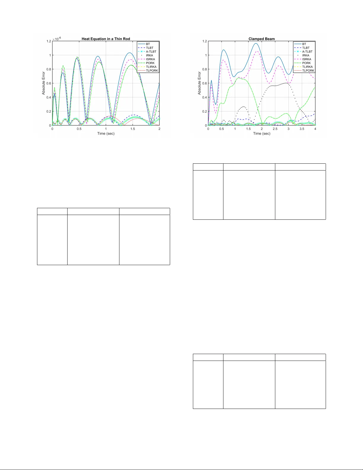
“ ”THIS P APER IS A PREPRINT OF A P APER ACCEPTED BY IET CONTR OL THEOR Y & APPLICA TIONS AND IS SUBJECT TO INSTITUTION OF ENGINEERING AND TECHNOLOGY COPYRIGHT .” 1 T ime-limited pseudo-optimal H 2 -model order reduction Umair Zulfiqar , V ictor Sreeram, and Xin Du Abstract —A model order reduction algorithm is presented that generates a reduced-order model of the original high- order model, which ensures high-fidelity within the desired time interv al. The reduced model satisfies a subset of the first- order optimality conditions for time-limited H 2 -model reduction problem. The algorithm uses a computationally efficient Krylov subspace-based framework to generate the reduced model, and it is applicable to large-scale systems. The reduced-order model is parameterized to enfor ce a subset of the first-order optimality conditions in an iteration-free way . W e also propose an adaptive framework of the algorithm, which ensures a monotonic decay in error irr espective of the choice of interpolation points and tangential directions. The efficacy of the algorithm is validated on benchmark model reduction problems. Index T erms — H 2 -norm, model reduction, optimal, time- limited. I . I N T R OD U C T I O N T HE intricacies and comple xity of the physical systems are increasing each year . The modern-day physical systems are mathematically described by se veral hundred or thousands of differential equations resulting in a large-scale state-space model. The computing power of the modern-day computers is also increasing at an increasing rate; howe ver , the complexity of the physical systems still poses a computational challenge to the efficient simulation, analysis, and design. Model order reduction (MOR) techniques are used to obtain a reduced- order approximation of the original high-order model, which retains most of its input-output properties. The reduced-order model (R OM) can then be used as a surrogate for the original high-order system in the design and analysis [1], [2], [3], [4], [5], [6]. Balanced truncation (BT) [7] is among the most popular MOR techniques. The preservation of stability , the existence of an a priori error bound, and high accuracy are among the most significant features of BT . In BT , the states which hav e significant Hankel singular values are retained in the R OM, and the remaining states are truncated. BT requires the solution of tw o lar ge-scale L yapunov equations which “This paper is a preprint of a paper accepted by IET Control Theory & Applications and is subject to Institution of Engineering and T echnology Copyright. When the final version is published, the copy of record will be av ailable at the IET Digital Library”. U. Zulfiqar and V . Sreeram are with the School of Electrical, Electronics and Computer Engineering, The University of W estern Australia, 35 Stirling Highway , Crawle y , W A 6009 (email: umair.zulfiqar@research.uw a.edu.au, victor .sreeram@uwa.edu.au). X. Du is with the School of Mechatronic Engineering and Automation, Shanghai Uni versity , Shanghai 200072, China, and also with the Shanghai K ey Laboratory of Power Station Automation T echnology , Shanghai Univ ersity , Shanghai 200444, P .R. China (e-mail: duxin@shu.edu.cn) is a computationally intensiv e task. The high computational cost of BT hinders its applicability to large-scale systems. Sev eral e xtensions of BT exist in the literature to reduce its computational cost like [8], [9], [10], [11], [12] which suggest replacing the exact solution of the L yapunov equations with their low-rank approximations. BT is generalized to preserve sev eral other system characteristics like passi vity , second-order structure, contractivity , etc. Reference [1] provides an in-depth surve y of BT and its extensions. The modal configuration is an important mathematical prop- erty of the system model, which is related to sev eral physical phenomena. For instance, the interconnected po wer systems exhibit low-frequenc y oscillations like local, interplant, and interarea oscillations. These are associated with the modes in the frequency interval of 0 − 2 Hz and are poorly damped [13]. The small-signal stability analysis and the damping controller design rely heavily on these modes. V arious modes can also be associated with the power system components in the network, like generators and power system stabilizers. Therefore, their preservation in the R OM is important from a physical perspectiv e. Moreov er, their preserv ation in the R OM is also beneficial for the accuracy of ROM both in the time and frequency domains [14], [15], [16], [17]. Recently , sev eral eigensolvers are developed which exploit the sparse structure of the large-scale models and ef ficiently compute the dominant modes [18], [19], [20] which are required to be preserved in the R OM for achieving good accuracy . Modal truncation based on these eigensolvers can ef ficiently generate a R OM for large-scale systems which preserv es the dominant modes of the original model. In terms of accuracy , modal truncation is way inferior to BT . Ho wev er, in many applications, the preserv ation of important modes of the original system is more important than the overall accuracy in terms of error . Moment matching is another important class of MOR tech- niques. In moment matching methods, a R OM is constructed which interpolates the original transfer function and a few of its moments using computationally ef ficient rational Krylov subspace based-framework. These techniques can easily han- dle large-scale systems and can be applied e ven if the model is unknown, and only the input-output data is known [21]. Moment matching methods have been significantly advanced ov er the last two decades, and several generalizations and extensions exist which can preserve various system properties while ensuring good accuracy as well. Reference [22] provides a detailed survey of moment matching methods. The H 2 -optimal MOR problem is studied extensi vely in the literature. One popular approach to this problem is to first con vert it into an unconstraint minimization problem “ ”THIS P APER IS A PREPRINT OF A P APER ACCEPTED BY IET CONTR OL THEOR Y & APPLICA TIONS AND IS SUBJECT TO INSTITUTION OF ENGINEERING AND TECHNOLOGY COPYRIGHT .” 2 ov er Stiefel manifold. Then the ROM is constructed using optimization schemes that minimize the cost function derived ov er the manifold [23], [24], [25]. In [26], a trust-region for the H 2 -optimal MOR over Stiefel manifold is proposed using the Riemannian trust-region method of [27]. In [28], the Rie- mannian trust-re gion method [27] is generalized for second- order transfer functions wherein the second-order structure is preserved in the R OM. The second popular approach to the H 2 -optimal MOR problem is the tangential interpola- tion. The first-order optimality conditions (known as W ilson’ s conditions [29]) are described as the tangential interpolation conditions in [30], [31]. The iterati ve rational Krylo v algorithm (IRKA) [30] is considered among the gold standards of these methods, and it efficiently generates a local optimum for the problem. IRKA was first developed for single-input single- output (SISO) systems in [30], and it is generally as accurate as BT ev en if it is initialized with fairly random interpolation points. It was later generalized for multi-input multi-output (MIMO) systems in [31]. IRKA is computationally efficient and thus easily applicable to large-scale systems. In general, the conv ergence is not guaranteed in IRKA, and it significantly slo ws do wn as the number of inputs and outputs increases. Moreover , the stability of the R OM is not guaranteed. There are some methods reported in the literature, which use trust-region methods to speed up the con ver gence of IRKA like [32], [33], [34]. In [35], a projection-based algorithm is proposed, which provides a sub-optimal solution to the H 2 -MOR problem while guaranteeing the stability of the R OM at the same time. The applicability of the algorithm [35] can also be extended to the nonlinear systems. The L yapunov equation-based algorithm presented in [36] also guarantees the stability of the ROM while preserving the second-order struc- ture in the R OM. Gugercin presented a modification to IRKA, i.e., iterativ e SVD rational Krylov algorithm (ISRKA), which satisfies a subset of the first-order optimality conditions for the H 2 -MOR problem, and the stability is also guaranteed [37]. Howe ver , the algorithm presented is an iterativ e algorithm with no guarantee on con vergence. Also, it requires the computation of one large-scale L yapunov equation which is computation- ally not feasible in a large-scale setting. In [38], an iteration- free pseudo-optimal rational Krylov (PORK) algorithm is presented, which generates a R OM that satisfies a subset of the first-order optimality conditions like ISRKA, and the R OM is also guaranteed to be stable. Unlike ISKRA, it does not require the solution of a lar ge-scale L yapunov equation, and thus it is computationally efficient. In [39], a cumulativ e reduction (CURE) framework is proposed, which constructs the R OM adaptiv ely . In each step, ne w interpolation conditions are enforced without affecting the conditions induced in the previous steps. An important property of CURE is that if PORK is used in it’ s ev ery step, the H 2 -norm error decays monotonically irrespecti ve of the choice of interpolation points and tangential directions. Practically , no system or its simulation is run ov er an infinite time interval. In some applications, a particular time interval is more important in terms of accuracy , e.g., the low-frequency oscillations in the interconnected po wer system are observed in the first 15 sec of the simulation, after which these are successfully damped by the power system stabilizers. The first 15 sec are very important for the small-signal stability analysis of the interconnected po wer systems [40]. Similarly , in a time-limited optimal control problem, the behavior of the system and the performance of the controller is important within a finite time interval [41]. It is, therefore, reasonable to ensure superior accuracy within the desired time interval of the interest. T o ensure high-fidelity in a desired limited time interval, BT is generalized to time-limited BT (TLBT) in [42]. TLBT is computationally expensi ve as it requires the solution of two large-scale dense L yapunov equations. In [43], the applicability of TLBT is extended to large- scale systems using Krylov subspace-based methods and lo w- rank approximation of large-scale L yapunov equations. The R OM is not guaranteed to be stable in TLBT , and an a priori error bound does not exist. In [44], a modification in TLBT is proposed, which guarantees stability , and an error bound is also defined. Howe ver , [44] is computationally more expensi ve than the original TLBT , and the accuracy is also poor . An H 2 -norm error bound for TLBT is also proposed in [45], which is based on the error bound in [46]. TLBT is extended to more general classes of linear systems in [47], [48], [49], [50] and bilinear systems in [51]. In [52], a cross Gramian based algorithm for TLBT is presented, which significantly sa ves the computational time as it requires one instead of two large-scale L yapunov equations. Further , TLBT is extended to unstable systems in [53]. In [54], IRKA is generalized to time-limited scenario to approximately achiev e the first-order optimality conditions for the time-limited H 2 - MOR problem. The first-order optimality conditions for the time-limited H 2 -MOR problem are expressed as bi-tangential Hermite interpolation conditions in [55], and a descent-based iterativ e algorithm is presented for the SISO systems. The algorithm [55] generates a R OM that satisfies these conditions for SISO system. It is computationally not feasible in a large- scale setting as it requires the computation of the pole-residue form of the original transfer function, which is an expensiv e task. Moreov er, the stability of the original system is not guaranteed to be preserved in the ROM generated by both the algorithms, and there is no guarantee on the conv ergence of the algorithms. In this paper , we present a time-limited MOR algorithm which satisfies a subset of the first-order optimality conditions for the time-limited H 2 -MOR problem (as deriv ed in [54] and [55]). The algorithm is iteration-free, and it guarantees the stability of R OM. The proposed algorithm does not in volve any large-scale L yapunov equation, and it uses a computationally efficient rational Krylov algorithm to construct the R OM. Therefore, it is applicable to large-scale systems. The proposed algorithm uses the parametrization of the R OM approach [56], [57] to enforce a subset of the optimality conditions and to place the poles and their associated input or output residues to the specified locations. Thus, it can also preserve the modes and their associated input or output residues of the original systems like modal truncation. Therefore, the proposed algorithm can also be used for the applications wherein modal preservation is an important property to be preserved in the ROM. W e also present an adaptive version “ ”THIS P APER IS A PREPRINT OF A P APER ACCEPTED BY IET CONTR OL THEOR Y & APPLICA TIONS AND IS SUBJECT TO INSTITUTION OF ENGINEERING AND TECHNOLOGY COPYRIGHT .” 3 of the algorithm, which ensures that the time-limited H 2 - norm error decays monotonically irrespectiv e of the choice of interpolation points and tangential directions. The proposed algorithm also provides approximate time-limited Gramians, which monotonically approach to the exact solutions. The approximate Gramians can be used for a computationally effi- cient implementation of TLBT . W e hav e tested our algorithm on benchmark MOR problems, and the simulation results confirm the efficacy of the proposed algorithm. I I . P R E L I M I N A R I E S Let H ( s ) be the n th order model of the original high-order system. The MOR problem is to find a r th ( r << n ) order R OM ˆ H r ( s ) of H ( s ) such that the error || H ( s ) − ˆ H r ( s ) || is small in some defined sense. Let x ∈ R n × 1 , u ∈ R 1 × m , and y ∈ R p × 1 be the state, input, and output vectors of the state-space representation of H ( s ) , i.e., ˙ x = Ax + B u, y = C x, H ( s ) = C ( sI − A ) − 1 B . (1) Let x r ∈ R r × 1 and y r ∈ R p × 1 be the state and output vectors of the state-space representation of ˆ H r ( s ) , i.e., ˙ x r = ˆ A r x r + ˆ B r u ˆ y r = ˆ C r x r . (2) ˆ W r and ˆ V r project H ( s ) onto a reduced subspace such that the dominant dynamics of H ( s ) are retained in ˆ H r ( s ) , i.e., ˆ H r ( s ) = C ˆ V r ( sI − ˆ W T r A ˆ V r ) − 1 ˆ W T r B = ˆ C r ( sI − ˆ A r ) − 1 ˆ B r . The time-limited MOR problem is to compute a R OM ( ˆ A r , ˆ B r , ˆ C r ) such that y ≈ ˆ y r within the desired time interval [0 , t ] sec. The important mathematical notations which are used throughout the text are tabulated in T able I. T ABLE I: Mathematical Notations Notation Meaning  .  ∗ Hermitian of the matrix tr ( · ) T race of the matrix λ i ( · ) Eigen values of the matrix Ran ( · ) Range of the matrix orth ( · ) Orthogonal basis for the range of the matrix span i =1 , ··· ,r {·} Span of the set of r vectors Let h ( t ) = C e At B and ˆ h r ( t ) = ˆ C r e ˆ A r t ˆ B r be the im- pulse responses of H ( s ) and ˆ H r ( s ) , respectively . The fourier transforms of h ( t ) and ˆ h r ( t ) are giv en by C F ( ω ) B and ˆ C r ˆ F ( ω ) ˆ B r , respectiv ely where F ( ω ) = ( j ω I − A ) − 1 and ˆ F ( ω ) = ( j ω I − ˆ A r ) − 1 . The controllability Gramian P and observability Gramian Q of the state-space realization ( A, B , C ) are defined as the following P = Z ∞ 0 e Aτ B B T e A T τ dτ = 1 2 π Z ∞ −∞ F ( ν ) B B T F ∗ ( ν ) dν (3) Q = Z ∞ 0 e A T τ C T C e Aτ dτ = 1 2 π Z ∞ −∞ F ∗ ( ν ) C T C F ( ν ) dν. (4) The time-limited controllability Gramian P T and the time- limited observability Gramain Q T defined ov er the time inter- val [0 , t ] [42] are defined as P T = Z t 0 e Aτ B B T e A T τ dτ Q T = Z t 0 e A T τ C T C e Aτ dτ . Similarly , the frequency-limited controllability Gramian P Ω and the frequency-limited observ ability Gramain Q Ω defined ov er the frequency interval [0 , ω ] [42] are defined as P Ω = 1 2 π Z ω − ω F ( ν ) B B T F ∗ ( ν ) dν (5) Q Ω = 1 2 π Z ω − ω F ∗ ( ν ) C T C F ( ν ) dν. (6) Definition 1. The H 2 -norm [30] of H ( s ) is defined as || H ( s ) || H 2 = s tr  Z ∞ 0 h ( τ ) h T ( τ ) dτ  = s tr  Z ∞ 0 C e Aτ B B T e A T τ C T dτ  = q tr  C P C T  = s tr  Z ∞ 0 h T ( τ ) h ( τ ) dτ  = s tr  Z ∞ 0 B T e A T τ C T C e Aτ B dτ  = q tr  B T QB  . Definition 2. The time-limited H 2 -norm [54] for the time interval [0 , t ] , i.e., H 2 ,t of H ( s ) is defined as || H ( s ) || H 2 ,t = s tr  Z t 0 h ( τ ) h T ( τ ) dτ  = s tr  Z t 0 C e Aτ B B T e A T τ C T dτ  = q tr  C P T C T  = s tr  Z t 0 h T ( τ ) h ( τ ) dτ  = s tr  Z t 0 B T e A T τ C T C e Aτ B dτ  = q tr  B T Q T B  . “ ”THIS P APER IS A PREPRINT OF A P APER ACCEPTED BY IET CONTR OL THEOR Y & APPLICA TIONS AND IS SUBJECT TO INSTITUTION OF ENGINEERING AND TECHNOLOGY COPYRIGHT .” 4 Definition 3. The frequency-limited H 2 -norm [58] for the frequency interval [0 , ω ] , i.e., H 2 ,ω of H ( s ) is defined as || H ( s ) || H 2 ,ω = s tr  1 2 π Z ω − ω H ( j ν ) H ∗ ( j ν ) dν  = s tr  1 2 π Z ω − ω C F ( ν ) B B T F ∗ ( ν ) C T dν  = q tr  C P Ω C T  = s tr  1 2 π Z ω − ω H ∗ ( j ν ) H ( j ν ) dν  = s tr  1 2 π Z ω − ω B T F ∗ ( ν ) C T C F ( ν ) B dν  = q tr  B T Q Ω B  . Definition 4. The H 2 ,t -norm [54] of the error system E ( s ) = H ( s ) − ˆ H r ( s ) is given by || E ( s ) || H 2 ,t = q tr ( C P T C T ) − 2 tr ( C ˜ P T ˆ C T r ) + tr ( ˆ C r ˆ P T ˆ C T r ) = q tr ( B T Q T B ) − 2 tr ( ˆ B T r ˜ Q T B ) + tr ( ˆ B T r ˆ Q T ˆ B r ) where AP T + P T A T + B B T − e At B B T e A T t = 0 , (7) A T Q T + Q T A + C T C − e A T t C T C e At = 0 , (8) ˆ A r ˆ P T + ˆ P T ˆ A T r + ˆ B r ˆ B T r − e ˆ A r t ˆ B r ˆ B T r e ˆ A T r t = 0 , (9) ˆ A T r ˆ Q T + ˆ Q T ˆ A r + ˆ C T r ˆ C r − e ˆ A T r t ˆ C T r ˆ C r e ˆ A r t = 0 , (10) A ˜ P T + ˜ P T ˆ A T r + B ˆ B T r − e At B ˆ B T r e ˆ A T r t = 0 , (11) ˆ A T r ˜ Q T + ˜ Q T A + ˆ C T r C − e ˆ A T r t ˆ C T r C e At = 0 . (12) See [54] for the proof. A. PORK [38] ˆ H r ( s ) interpolates H ( s ) at the interpolation points σ i in the respective (right) tangential directions ˆ c i ∈ C m × 1 for any output rational Krylov subspace ˆ W r such that ˆ W T r ˆ V r = I if the input rational Krylov subspace ˆ V r satisfies the following property Ran ( ˆ V r ) = span i =1 , ··· ,r { ( σ i I − A ) − 1 B ˆ c i } . (13) Choose ˆ W r as ˆ W r = ˆ V r ( ˆ V r ˆ V T r ) − 1 , and compute the follo wing matrices ˆ A r = ˆ W T r A ˆ V r , ˆ B r = ˆ W T r B , (14) B ⊥ = B − ˆ V r ˆ B r , (15) ˆ L r = ( B T ⊥ B ⊥ ) − 1 B T ⊥  A ˆ V r − ˆ V r ˆ A r  , (16) ˆ S r = ˆ A r − ˆ B r ˆ L r . (17) Then ˆ V r satisfies the following Sylvester equations: A ˆ V r + ˆ V r ( − ˆ S r ) + B ( − ˆ L r ) = 0 , (18) A ˆ V r + ˆ V r ( − ˆ A r ) + B ⊥ ( − ˆ L r ) = 0 (19) where { σ 1 , · · · , σ r } are the eigen values of ˆ S r . A family of R OMs which satisfy the interpolation condition ˆ H r ( σ i )ˆ c i = H ( σ i )ˆ c i (20) can be obtained by parametrizing the R OM in ˆ B r if all the interpolation points σ i hav e positi ve real parts, and ( ˆ S r , ˆ L r ) is observable, i.e., ˆ A r = ˆ S r + ξ ˆ L r , ˆ B r = ξ , ˆ C r = C ˆ V r . ˆ H r ( s ) ensures that || H ( s ) − ˆ H r ( s ) || 2 H 2 = || H ( s ) || 2 H 2 − || ˆ H r ( s ) || 2 H 2 (21) if ξ is set to ξ = − ˆ Q − 1 s ˆ L T r where ˆ Q s solves − ˆ S T r ˆ Q s − ˆ Q s ˆ S r + ˆ L T r ˆ L r = 0 . The equation (21) is a subset of the first-order optimality con- ditions for the local optimality problem || H ( s ) − ˆ H r ( s ) || 2 H 2 , and thus ˆ H r ( s ) is a pseudo-optimal ROM of H ( s ) . B. CURE [39] The r th -order R OM in CURE is constructed adaptiv ely in k steps. ( ˆ A r , ˆ B r , ˆ C r ) , ˆ S r , ˆ L r , and B ⊥ are accumulated after each step such that the interpolation condition (20), and the Sylvester equations (18) and (19) are satisfied after each step. In other words, at each step, new interpolation points and the tangential directions are added without disturbing the interpolation conditions induced by the previous interpolation points and tangential directions. Let ˆ V ( k ) , ˆ S ( k ) , ˆ L ( k ) , ( ˆ A ( k ) , ˆ B ( k ) , ˆ C ( k ) ) , and B ( k ) ⊥ be matrices of k th step for any ˆ W ( k ) such that ( ˆ W ( k ) ) T ˆ V ( k ) = I , i.e., ˆ A ( k ) = ( ˆ W ( k ) ) T A ˆ V ( k ) , ˆ B ( k ) = ( ˆ W ( k ) ) T B ( k − 1) ⊥ , ˆ C ( k ) = C ˆ V ( k ) where A ˆ V ( k ) − ˆ V ( k ) ˆ S ( k ) − B ( k − 1) ⊥ ˆ L ( k ) = 0 , (22) A ˆ V ( k ) − ˆ V ( k ) ˆ A ( k ) − B ( k ) ⊥ ˆ L ( k ) = 0 , (23) B (0) ⊥ = B , and B ( k ) ⊥ = B ( k − 1) ⊥ − ˆ V ( k ) ˆ B ( k ) . After each step, the R OM can be accumulated, and a r th -order R OM can be obtained adaptively in k steps, i.e., the order of the R OM grows after each step without affecting the interpola- tion conditions induced in the previous steps. The accumulated R OM and the associated matrices for i = 1 , · · · , k are giv en by A ( i ) tot =    A ( i − 1) tot 0 ˆ B ( i ) L ( i − 1) tot ˆ A ( i )    , B ( i ) tot =   B ( i − 1) tot ˆ B ( i )   , C ( i ) tot = h C ( i − 1) tot ˆ C ( i ) i , L ( i ) tot = h L ( i − 1) tot ˆ L ( i ) i , S ( i ) tot =   S ( i − 1) tot − B ( i − 1) tot ˆ L ( i ) 0 ˆ S ( i )   , V ( i ) tot = h V ( i − 1) tot ˆ V ( i ) i “ ”THIS P APER IS A PREPRINT OF A P APER ACCEPTED BY IET CONTR OL THEOR Y & APPLICA TIONS AND IS SUBJECT TO INSTITUTION OF ENGINEERING AND TECHNOLOGY COPYRIGHT .” 5 where AV ( i ) tot − V ( i ) tot S ( i ) tot − B L ( i ) tot = 0 , and A (0) tot , B (0) tot , C (0) tot , L (0) tot , S (0) tot , and V (0) tot are all empty matrices. An important property of CURE is that if ( ˆ A ( i ) , ˆ B ( i ) , ˆ C ( i ) ) is computed using PORK for i = 1 , · · · , k , ( A ( i ) tot , B ( i ) tot , C ( i ) tot ) stays pseudo-optimal. This further implies that ( A ( i − 1) tot , B ( i − 1) tot , C ( i − 1) tot ) is a pseudo-optimal R OM of ( A ( i ) tot , B ( i ) tot , C ( i ) tot ) as S ( i ) tot and ˆ C ( i ) tot contain the interpolation points and tangential directions encoded in S ( i − 1) tot and ˆ C ( i − 1) tot , respectiv ely . Let H ( i ) tot  s  be defined as H ( i ) tot  s  = C ( i ) tot ( sI − A ( i ) tot ) − 1 B ( i ) tot . If H ( i ) tot  s  stays pesudo-optimal, the following holds || H ( s ) − H ( i ) tot  s  || 2 H 2 = || H ( s ) || 2 H 2 − || H ( i ) tot  s  || 2 H 2 . Thus || H ( s ) || 2 H 2 ≥ || H ( i ) tot  s  || 2 H 2 . Moreover , since || H ( i ) tot  s  − H ( i − 1) tot  s  || 2 H 2 = || H ( i ) tot  s  || 2 H 2 − || H ( i − 1) tot  s  || 2 H 2 , || H ( i ) tot  s  || 2 H 2 ≥ || H ( i − 1) tot  s  || 2 H 2 . Therefore, || H ( s ) − H ( i ) tot  s  || 2 H 2 decays monotonically irrespectiv e of the choice of interpolation points and tangential directions. C. TLBT [42] TLBT [42] is a generalization of BT [7] wherein the standard controllability and observability Gramians, which are defined ov er the infinite time horizon, are replaced with the ones defined over the time interv al of interest. ˆ V r and ˆ W r in TLBT are computed as ˆ V r = ˆ T r ˆ R T r and ˆ W r = ˆ T − T r ˆ R T r , respectiv ely , where ˆ R r =  I r × r 0 r × ( n − r )  , ˆ T − 1 r P T ˆ T − T r = ˆ T T r Q T ˆ T r = diag ( ˆ σ 1 , ˆ σ 2 , · · · , ˆ σ n ) , and ˆ σ 1 ≥ ˆ σ 2 ≥ · · · ≥ ˆ σ n . The ROM is then obtained as ˆ A r = ˆ W T r A ˆ V r , ˆ B r = ˆ W T r B , ˆ C r = C ˆ V r . D. H 2 ,t -Optimal MOR Define G ( s ) and ˆ G r ( s ) as the following G ( s ) = − e − st f C ( sI − A ) − 1 e At f B + H ( s ) , (24) ˆ G r ( s ) = − e − st f ˆ C r ( sI − ˆ A r ) − 1 e ˆ A r t f ˆ B r + ˆ H r ( s ) . (25) Let ˆ H r ( s ) be represented in the following pole-residue form ˆ H r ( s ) = r X k =1 ˆ l k ˆ r T k s − ˆ λ k . (26) It is sho wn in [55] that ˆ H r ( s ) is a local optimum for the problem || H ( s ) − ˆ H r ( s ) || 2 H 2 ,t if the following bi-tangential Hermite interpolation conditions are satisfied ˆ l T k G ( − ˆ λ k ) = ˆ l T k ˆ G r ( − ˆ λ k ) (27) G ( − ˆ λ k ) ˆ r k = ˆ G r ( − ˆ λ k ) ˆ r k (28) ˆ l T k G 0 ( − ˆ λ k ) ˆ r k = ˆ l T k ˆ G 0 r ( − ˆ λ k ) ˆ r k . (29) Further , it is shown in [54] that these are equiv alent to the following Gramian-based first-order optimality conditions ˆ C r ˆ P T = C ˜ P T (30) ˆ Q T ˆ B r = ˜ Q T B (31) ˆ e ∗ i ˜ X ∞ [ ˜ P T − te At B ˆ B ∗ r e ˆ A ∗ r t ] ˆ e i = ˆ e ∗ i ˆ Q ∞ [ ˆ P T − te ˆ A r t ˆ B r ˆ B ∗ r e ˆ A ∗ r t ] ˆ e i (32) where ˆ A r ˜ X ∞ + ˜ X ∞ A ∗ + ˆ C ∗ r C = 0 , ˆ A ∗ r ˆ Q ∞ + ˆ Q ∞ ˆ A r + ˆ C ∗ r ˆ C r = 0 , and ˆ e i is the unit vector . When either the equation (30) or (31) (or equiv alently the equation (27) or (28)) is satisfied, the following holds || H ( s ) − ˆ H r ( s ) || 2 H 2 ,t = || H ( s ) || 2 H 2 ,t − || ˆ H r ( s ) || 2 H 2 ,t . (33) E. Issues in H 2 ,t -Optimal MOR ˆ H r ( s ) and resultantly { ˆ λ k , ˆ l k , ˆ r k } k =1 , ··· ,r are not known a priori which necessitate an iterativ e algorithm starting with a random guess of the interpolation data. The bi-tangential Hermite interpolation conditions (27)-(29) cannot be achiev ed if IRKA is applied to G ( s ) . Note that a ROM of G ( s ) is not required. A R OM ˆ H r ( s ) is required which satisfies (27)- (29). If IRKA is applied to G ( s ) , there is no way to e xtract ˆ H r ( s ) from ˆ G r ( s ) as IRKA cannot preserve the structure of ˆ G r ( s ) according to (25). In [55], a decent algorithm is presented for SISO systems which computes ˆ H r ( s ) which satisfies G ( − ˆ λ k ) = ˆ G r ( − ˆ λ k ) and G 0 ( − ˆ λ k ) = ˆ G 0 r ( − ˆ λ k ) using quasi-Newton type optimization. This is a computationally expensi ve strategy to achieve the optimality conditions, which is just limited to the SISO systems. In [54], a projection-based algorithm the time-limited IRKA (TLIRKA) is presented, which tends to achiev e optimality conditions (30)-(32). The algorithm does not achiev e an exact local optimum; ne vertheless, it yields a R OM, which ex- hibits high-fidelity within the specified time interval [0 , t ] . Let ( ˆ A r , ˆ B r , ˆ C r ) be the initial guess of the ROM, and let QS Q − 1 be the spectral factorization of ˆ A r , B = S ˆ B r , and C = ˆ C r S − 1 where Q =  q 1 · · · q r  and q i is the eigen vector of λ i ( ˆ A r ) . The algorithm in [54] heuristically suggests replacing B B ∗ and C ∗ C in IRKA with B B ∗ − e At B B ∗ e S t and C ∗ C − e A ∗ t C ∗ C e S t , respectiv ely for the calculation of the reduction subspaces (see the equations (34)-(35)). The input and output subspaces in TLIRKA [54] are computed as A ˆ V r,t + ˆ V r,t S + B B ∗ − e At B B ∗ e S t = 0 , (34) A ∗ ˆ W r,t + ˆ W r,t S + C ∗ C − e A ∗ t C ∗ C e S t = 0 . (35) ˆ V r,t and ˆ W r,t is set to or th ( ˆ V r,t ) and orth ( ˆ W r,t ) , respectiv ely , and the ROM is updated as ˆ A r = ( ˆ W ∗ r,t ˆ V r,t ) − 1 ˆ W ∗ r,t A ˆ V r,t , ˆ B r = ( ˆ W ∗ r,t ˆ V r,t ) − 1 ˆ W ∗ r,t B , ˆ C r = C ˆ V r,t . The process is repeated until the relati ve change in S stagnates. W e will explain in the next section why this simple heuristic “ ”THIS P APER IS A PREPRINT OF A P APER ACCEPTED BY IET CONTR OL THEOR Y & APPLICA TIONS AND IS SUBJECT TO INSTITUTION OF ENGINEERING AND TECHNOLOGY COPYRIGHT .” 6 modification in IRKA generates a high-fidelity ROM despite the fact that it does not achieve the optimality conditions (30)- (32). Here we just mention that TLIRKA tends to achieve (30) and (31) upon conv ergence; howe ver , it fails to do so because a particular structure is required to be preserved in the R OM, which is not possible in an IRKA-type framew ork. Moreover , the con ver gence is not guaranteed in both the aforementioned approaches. I I I . M A I N R E S U LT S In this section, we present an iteration-free rational Krylov subspace based MOR algorithm, which generates a time- limited pseudo-optimal R OM of H ( s ) . W e call a ROM as time-limited pseudo-optimal if it satisfies (33). The ROM thus satisfies a subset of the optimality conditions for the problem || H ( s ) − ˆ H r ( s ) || 2 H 2 ,t , i.e., ˆ H r ( s ) satisfies either (30) or (31). W e name our algorithm as “time-limited PORK (TLPORK)”. W e then generalize CURE such that || H ( s ) − ˆ H r ( s ) || 2 H 2 ,t decays monotonically after each step irrespective of the choice of interpolation points and tangential directions, and we name it as “time-limited CURE (TLCURE)”. A. TLPORK Let us define H T ( s ) , G T ( s ) , ˆ H T r ( s ) , and ˆ G T r ( s ) as the following H T ( s ) = C ( sI − A ) − 1 B T , G T ( s ) = C T ( sI − A ) − 1 B , ˆ H T r ( s ) = ˆ C r ( sI − ˆ A r ) − 1 ˆ B T r , ˆ G T r ( s ) = ˆ C T r ( sI − ˆ A r ) − 1 ˆ B r where B T =  B − e At B  , ˆ B T r = h ˆ B r − e ˆ A r t ˆ B r i , (36) C T =  C − C e At  , and ˆ C T r = " ˆ C r − ˆ C r e ˆ A r t # . (37) W e begin our in vestigation by finding out the reason why TLIRKA constructs a nearly-optimal R OM due to the heuristic choice of the reduction subspaces proposed in [54]. Intuitively , it appears that TLIRKA tries to satisfy the following interpo- lation conditions H T ( ˆ λ k ) r k = ˆ H T r ( − ˆ λ k ) r k , (38) l T k G T ( − ˆ λ k ) = l T k ˆ G T r ( − ˆ λ k ) (39) while maintaining the structure of ˆ B T r and ˆ C T r where  ˆ r 1 · · · ˆ r r  ˆ r 1 · · · ˆ r r  e diag ( ˆ λ 1 , ··· , ˆ λ r ) t  =  r 1 . . . r r  ,    ˆ l 1 . . . ˆ l r e diag ( ˆ λ 1 , ··· , ˆ λ r ) t    ˆ l 1 . . . ˆ l r       =    l 1 . . . l r    . Howe ver , it does not retain that structure because this is not possible in an IRKA-type frame work. Our first aim is to construct a R OM, which satisfies (38) or (39) while main- taining the structure of ˆ B T r or ˆ C T r according to (36) or (37), respectiv ely . The next aim is to study the properties of such ROM and in vestigate its connection with the optimality conditions (30)-(32). Let us define ˆ S r , ˆ L r , and L T as ˆ S r = diag ( σ 1 , · · · , σ r ) , ˆ L r =  ˆ c 1 · · · ˆ c r  , L T = " ˆ L r ˆ L r e − ˆ S t # =  c 1 . . . c r  . (40) ˆ H T ,r ( s ) interpolates H T ( s ) at the interpolation points σ k in the respective (right) tangential directions c k ∈ C 2 m × 1 for any output rational Krylov subspace ˆ W r,t such that ˆ W ∗ r,t ˆ V r,t = I if the input rational Krylov subspace ˆ V r,t is defined as ˆ V r,t =  ( A − σ 1 I ) − 1 B T c 1 · · · ( A − σ r I ) − 1 B T c r  . Owing to the relation with the Sylvester equation [39], ˆ V r,t solves the following Sylvester equation A ˆ V r,t + ˆ V r,t ( − ˆ S r ) + B T ( − L T ) = 0 . (41) A family of R OMs, which satisfy the interpolation condition ˆ H T r ( σ k ) c k = H T ( σ k ) c k , can be obtained by parametrizing ˆ H T r ( σ k ) in ˆ B T if all the interpolation points σ k hav e positiv e real parts, and ( ˆ S r , L T ) is observable, i.e., ˆ A r = ˆ S r + ξ L T ˆ B T = ξ ˆ C r = C ˆ V r,t . This can be v erified by multiplying (41) with ˆ W ∗ r,t from the left; see [39] for more details. The assumption on the interpolation points to have positiv e real parts is to ensure that the R OM is stable as we aim to place the poles at their mirror images, and the assumption on the observability of the pair ( ˆ S r , L T ) is to ensure that the pole-placement is possible. W e now propose a nov el choice of ξ which retains the structure of ˆ B T r according to the equation (36), i.e., ξ = h − ˆ Q − 1 S ˆ L ∗ r ˆ Q − 1 S e − ˆ S ∗ r t ˆ L ∗ r i (42) where − ˆ S ∗ r ˆ Q S − ˆ Q S ˆ S r + ˆ L ∗ r ˆ L r − e − ˆ S ∗ r t ˆ L ∗ r ˆ L r e − ˆ S r t = 0 . (43) ˆ H T r ( s ) is then obtained as ˆ A r = ˆ S r + ξ L T , ˆ B T ,r = ξ , ˆ C r = C ˆ V r,t . (44) ˆ H r ( s ) can be extracted from ˆ H T r ( s ) by setting ˆ B r = − ˆ Q − 1 S ˆ L ∗ r . This particular choice of ξ places the poles of ˆ H T r ( s ) (and ˆ H r ( s ) ) at the mirror images of the interpolation points and makes the tangential directions their respectiv e input-residuals. Thus, it enforces the interpolation condition (38) while also maintaining the structure of ˆ B T r according to (36). W e now prove these properties in the following theorem, and we also show that the R OM ˆ H r ( s ) obtained by enforcing these conditions is a time-limited pseudo-optimal R OM of H ( s ) . Theor em 1: If ( ˆ A r , ˆ B T ,r , ˆ C r ) is defined as in the equation (44), then ˆ H r ( s ) , which is extracted from ˆ H T r ( s ) by setting ˆ B r = − ˆ Q − 1 S ˆ L ∗ r , has the following properties: (i) ˆ H r ( s ) has poles at the mirror images of the interpolation points. “ ”THIS P APER IS A PREPRINT OF A P APER ACCEPTED BY IET CONTR OL THEOR Y & APPLICA TIONS AND IS SUBJECT TO INSTITUTION OF ENGINEERING AND TECHNOLOGY COPYRIGHT .” 7 (ii) ˆ c i is the input-residuals of the pole − σ ∗ i of ˆ H r ( s ) . (iii) ξ = h ˆ B r − e ˆ A r t ˆ B r i . (iv) ˆ Q − 1 S is the time-limited controllability Gramian of the pair ( ˆ A r , ˆ B r ) . (v) ˆ H r ( s ) is a time-limited pseudo-optimal ROM of H ( s ) . Proof . (i) By multiplying ˆ Q − 1 S from the left side of the equation (43) yields − ˆ Q − 1 S ˆ S ∗ r ˆ Q S − ˆ S r + ˆ Q − 1 S ˆ L ∗ r ˆ L r − ˆ Q − 1 S e − ˆ S ∗ r t ˆ L ∗ r ˆ L r e − ˆ S r t = 0 − ˆ Q − 1 S ˆ S ∗ r ˆ Q S − ˆ A r = 0 . Thus, ˆ A r = − ˆ Q − 1 S ˆ S ∗ r ˆ Q S , and hence, λ i ( ˆ A r ) = − λ i ( ˆ S ∗ r ) . (ii) ( − ˆ Q − 1 S )( − ˆ S ∗ r )( − ˆ Q S ) is actually the spectral factorization of ˆ A r . Also, ˆ B r = − ˆ Q − 1 S  ˆ c i · · · ˆ c r  ∗ . Thus, ˆ c i is the input-residual of − σ ∗ i . (iii) By putting the v alue of ˆ B r in h ˆ B r − e ˆ A r t ˆ B r i , we get h − ˆ Q − 1 S ˆ L ∗ r e ˆ A r t ˆ Q − 1 S ˆ L ∗ r i . Since, ˆ Q S e ˆ A r t ˆ Q − 1 S = e − ˆ S ∗ r t and e ˆ A r t ˆ Q − 1 S = ˆ Q − 1 S e − ˆ S ∗ r t , ξ = h ˆ B r − e ˆ A r t ˆ B r i . (iv) The time-limited controllability Gramian of ( ˆ A r , ˆ B r ) solves the following L yapunov equation (as in the equation (9)) ˆ A r ˆ P T + ˆ P T ˆ A ∗ r + ˆ B r ˆ B ∗ r − e ˆ A r t ˆ B r ˆ B ∗ e ˆ A ∗ r t = 0 . By pre- and post-multiplying the equation (9) with ˆ Q S , by putting ˆ A r = − ˆ Q − 1 S ˆ S ∗ r ˆ Q S and ˆ B r = − ˆ Q − 1 S ˆ L ∗ r , and also by noting that ˆ Q S e ˆ A r t ˆ Q − 1 S = e − ˆ S ∗ r t , the equation (9) becomes − ˆ S ∗ r ˆ Q S ˆ P T ˆ Q S − ˆ Q S ˆ P T ˆ Q S ˆ S r + ˆ L ∗ r ˆ L r − e − ˆ S ∗ r t ˆ L ∗ r ˆ L r e − ˆ S r t = 0 . Due to uniqueness, ˆ Q S ˆ P T ˆ Q S = ˆ Q S , ˆ Q S ˆ P T = I , and ˆ P T = ˆ Q − 1 S . (v) Consider the following equation A ˆ V r,t ˆ P T + ˆ V r,t ˆ P T ˆ A ∗ r + B ˆ B ∗ r − e At B ˆ B ∗ r e ˆ A ∗ r t = [ ˆ V r,t ˆ S r + B T L T ] ˆ P T − ˆ V r,t ˆ S r ˆ Q − 1 S − B ˆ L r ˆ Q − 1 S − e At B ˆ L r ˆ Q − 1 S e ˆ A ∗ r t = ˆ V r,t ˆ S r ˆ P T + B ˆ L r ˆ P T − e At B ˆ L r e − ˆ S r t ˆ P T − ˆ V r,t ˆ S r ˆ P T − B ˆ L r ˆ P T + e At B ˆ L r e − ˆ S r t ˆ P T = 0 . Due to uniqueness, ˆ V r,t ˆ P T = ˜ P T , and therefore, ˆ C r ˆ P T = C ˜ P T . Hence, ˆ H r ( s ) is a time-limited pseudo- optimal model ROM of H ( s ) . W e now aim to construct a ROM ˆ G T ,r ( s ) , which satisfies the interpolation condition (39) while preserving the structure of ˆ C T ,r according to (37). Let σ k be the interpolation points in the (left) tangential directions ˆ b k ∈ C 1 × p . Let us define ¯ B T and ˜ B T as ¯ B T =  ˆ b ∗ 1 · · · ˆ b ∗ r  ∗ , ˜ B T = h ¯ B T e − ˆ S r t ¯ B T i =  b ∗ 1 · · · b ∗ r  ∗ . (45) ˆ G T ,r ( s ) interpolates G T ( s ) at the interpolation points σ k in the respective (left) tangential directions b k ∈ C 2 m × 1 for any input rational Krylov subspace ˆ V r,t such that ˆ W ∗ r,t ˆ V r,t = I if the output rational Krylov subspace ˆ W r,t is defined as ˆ W r,t =  ( A ∗ − σ 1 I ) − 1 C ∗ T b ∗ 1 · · · ( A ∗ − σ r I ) − 1 C ∗ T b ∗ r  . Owing to the relation with the Sylvester equation [39], ˆ W r,t solves the following Sylvester equation ˆ W ∗ r,t A + ( − ˆ S r ) ˆ W ∗ r,t + ( − ˜ B T )( ˜ L T ) = 0 . (46) A family of ROMs which satisfy the interpolation condition b T k ˆ G T r ( σ k ) = b T k G T ( σ k ) can be obtained by parametrizing ˆ G T r ( σ k ) in ˆ C T ,r if all the interpolation points σ i hav e positiv e real parts, and the pair ( ˆ S r , ˜ B T ) is controllable, i.e., ˆ A r = ˆ S r + ˜ B T ξ , ˆ B r = ˆ W ∗ r,t B , ˆ C T ,r = ξ . (47) W e no w propose a no vel choice of ξ which retains the structure of ˆ C T r according to the equation (37), i.e., ξ = " − ¯ B ∗ T ˆ P − 1 S ¯ B ∗ T e − ˆ S ∗ r ˆ P − 1 S # , (48) where ˆ P S solves − ˆ S r ˆ P S − ˆ P S ˆ S ∗ r + ¯ B T ¯ B ∗ T − e − ˆ S r ¯ B T ¯ B ∗ T e − ˆ S ∗ r t = 0 . (49) ˆ H r ( s ) can be extracted from ˆ G T r ( s ) by setting ˆ C r = − ¯ B ∗ T ˆ P − 1 S . This particular choice of ξ places the poles of ˆ H r ( s ) at the mirror images of the interpolation points and makes the tangential directions their respecti ve output- residuals. Thus, it enforces the interpolation condition (39) while also maintaining the structure of ˆ C T r according to (37). W e now prove these properties in the following theorem, and we also show that the R OM ˆ H r ( s ) obtained by enforcing these conditions is a time-limited pseudo-optimal ROM of H ( s ) . Theor em 2: If ( ˆ A r , ˆ B r , ˆ C T ,r ) is defined as in the equation (47), then ˆ H r ( s ) , which is extracted from ˆ G T r ( s ) by setting ˆ C r = − ¯ B ∗ T ˆ P − 1 S , has the following properties: (i) ˆ H r ( s ) has poles at the mirror images of the interpolation points. (ii) ˆ b i is the output residual of the pole − σ ∗ i . (iii) ξ = " ˆ C r − ˆ C r e ˆ A r t # . (iv) ˆ P − 1 S is the time-limited observability Gramian of the pair ( ˆ A r , ˆ C r ) . (v) ˆ H r ( s ) is a time-limited pseudo-optimal ROM of H ( s ) . Proof . (i) By multiplying ˆ P − 1 S from the right, the equation (49) becomes − ˆ S r − ˆ P S ˆ S ∗ r ˆ P − 1 S + ¯ B T ¯ B ∗ T ˆ P − 1 S − e − ˆ S r ¯ B T ¯ B ∗ T e − ˆ S ∗ r t ˆ P − 1 S = 0 − ˆ P S ˆ S ∗ r ˆ P − 1 S − ˆ A r = 0 . Thus, ˆ A r = − ˆ P S ˆ S ∗ r ˆ P − 1 S , and hence, λ i ( ˆ A r ) = − λ i ( ˆ S ∗ r ) . (ii) ( − ˆ P S )( − ˆ S r )( − ˆ P − 1 S ) is actually the spectral factorization of ˆ A r . Moreov er, ˆ C r =  ˆ b ∗ 1 · · · ˆ b ∗ r  ( − ˆ P − 1 S ) . Thus, ˆ b i is the output residual of − σ ∗ i . (iii) By putting the value of ˆ C r in " ˆ C r − ˆ C r e ˆ A r t # , we get “ ”THIS P APER IS A PREPRINT OF A P APER ACCEPTED BY IET CONTR OL THEOR Y & APPLICA TIONS AND IS SUBJECT TO INSTITUTION OF ENGINEERING AND TECHNOLOGY COPYRIGHT .” 8 " − ¯ B ∗ T ˆ P − 1 S ¯ B ∗ T ˆ P − 1 S e ˆ A r t # . Since ˆ P − 1 S e ˆ A r t ˆ P S = e − ˆ S ∗ r t and ˆ P − 1 S e ˆ A r t = e − ˆ S ∗ r t ˆ P − 1 S , ξ = " ˆ C r − ˆ C r e ˆ A r t # . (iv) The time-limited observ ability Gramian of ( ˆ A r , ˆ C r ) solves the following L yapunov equation (as in the equation (10)) ˆ A ∗ r ˆ Q T + ˆ Q T ˆ A r + ˆ C ∗ r ˆ C r − e ˆ A ∗ r t ˆ C ∗ r ˆ C r e ˆ A r t = 0 . By pre- and post-multiplying the equation (10) with ˆ P S , by putting ˆ A r = − ˆ P S ˆ S ∗ r ˆ P − 1 S and ˆ C r = − ¯ B ∗ T ˆ P − 1 S , and also by noting that ˆ P − 1 S e ˆ A r t ˆ P S = e − ˆ S ∗ r t , the equation (10) becomes − ˆ S r ˆ P S ˆ Q T ˆ P S − ˆ P S ˆ Q T ˆ P S ˆ S ∗ r + ¯ B T ¯ B ∗ T − e − ˆ S r ¯ B T ¯ B ∗ T e − ˆ S ∗ r t = 0 . Due to uniqueness, ˆ P S ˆ Q T ˆ P S = ˆ P S , ˆ P S ˆ Q T = I , and ˆ Q T = ˆ P − 1 S . (v) Consider the following equation ˆ A ∗ r ˆ Q T ˆ W ∗ r,t + ˆ Q T ˆ W ∗ r,t A + ˆ C ∗ r C − e ˆ A ∗ r t ˆ C ∗ r C e At = − ˆ Q T ˆ S r ˆ W ∗ r,t + ˆ Q T [ ˆ S r ˆ W ∗ r,t + ˜ B T ˜ L T ] − ˆ Q T ¯ B T C + e ˆ A ∗ r t ˆ Q T ¯ B T C e At = − ˆ Q T ˆ S r ˆ W ∗ r,t + ˆ Q T ˆ S r ˆ W ∗ r,t + ˆ Q T ¯ B T C − ˆ Q T e − ˆ S r t ¯ B T C e At − ˆ Q T ¯ B T C + e ˆ A ∗ r t ˆ Q T ¯ B T C e At =0 Due to uniqueness, ˆ Q T ˆ W ∗ r,t = ˜ Q T , and therefore, ˆ Q T ˆ B r = ˜ Q T B . Hence, ˆ H r ( s ) is a time-limited pseudo-optimal model R OM of H ( s ) . Remark 1: If the interpolation points are selected as the mirror images of r -poles of H ( s ) , TLPORK and O-TLPORK preserve these poles in ˆ H r ( s ) like modal truncation. Addition- ally , TLPORK and O-TLPORK preserve the input and output residues, respectively of these poles if the tangential directions are selected as such. Remark 2: TLPORK and O-TLPORK resemble PORK in its pole-placement property , i.e., they place the poles at the mirror images of the interpolation points and make the tangential directions residuals of the poles. Howe ver , PORK does not (and does not have to) preserve a structure in the R OM. Unlike PORK, TLPORK and O-TLPORK do (and have to) preserve a specific structure in the R OM in order to satisfy the optimality conditions. When t is set to ∞ , TLPORK and O-TLPORK reduce to PORK. Remark 3: TLPORK and O-TLPORK satisfy the optimality conditions (30) and (31), respectiv ely , which are equiv alent to (27) and (28), respecti vely . For SISO systems, the interpolation conditions (27) and (28) are equiv alent. For MIMO systems, the interpolation conditions (27) and (28) are not equiv alent. Howe ver , the R OMs constructed by TLPORK and O-TLPORK both satisfy (33). The accuracy of the ROMs in the MIMO case depends on the choice of tangential directions, ev en if the interpolation points used in TLPORK and O-TLPORK are the same. Remark 4: The time-limited pseudo-optimality (equation (33)) does not depend on the realization of H ( s ) or ˆ H r ( s ) . B. Algorithmic Aspects W e allowed the state-space matrices to be complex so far in this section; howe ver , one can obtain a real R OM for a real original model if the complex interpolation points (and the associated tangential directions) are chosen in conjugate pairs. This is a standard practice in Krylov subspace methods wherein the interpolation data is grouped into conjugate pairs to obtain a real basis (which satisfies the property in the equation (50)); see [59] for more details. For instance, a real ˆ V r,t can be computed by any rational Krylov subspace method instead of actually solving the Sylvester equation (41), i.e., Ran ( ˆ V r,t ) = span i =1 , ··· ,r { ( σ i I − A ) − 1 B T c i } . (50) The next step then is to compute the matrices of Sylvester equation which this ˆ V r,t satisfies (as it may not satisfy the equation (41)). This can be accomplished in a few simple steps. Choose an y ˆ W r,t , for instance, ˆ W r,t = ˆ V r,t . Then compute the following matrices ˜ E = ˆ W T r,t ˆ V r,t , ˜ A = ˆ W T r,t A ˆ V r,t , ˜ B = ˆ W T r,t B T , (51) B ⊥ = B T − ˆ V r,t ˜ E − 1 ˜ B . (52) Then L T and ˆ S r for the Sylvester equation of this ˆ V r,t can be computed as L T = ( B T ⊥ B ⊥ ) − 1 B T ⊥  A ˆ V r,t − ˆ V r,t ˜ E − 1 ˜ A  , (53) ˆ S r = ˜ E − 1  ˜ A − ˜ B L T  . (54) Now partition L T as L T =  L + m × r L − m × r  , and define L − T as L − T =  L + m × r − L − m × r  . Then ˆ Q S can be computed from the following L yapunov equation − ˆ S T r ˆ Q S − ˆ Q S ˆ S r + L T T L − T = 0 . (55) Finally , the ROM is obtained as ˆ A r = − ˆ Q − 1 S ˆ S T r ˆ Q S , ˆ B r = − ˆ Q − 1 S ( L + m × r ) T , ˆ C r = C ˆ V r,t . (56) Algorithm 1: TLPORK Input: Original model: ( A, B , C ) , interpolation points: { σ 1 , · · · , σ r } , tangential directions: { ˆ c 1 , · · · , ˆ c r } . Output: ROM: ( ˆ A r , ˆ B r , ˆ C r ) . (i) Define B T according to the equation (36), and ˆ S r and L T according to the equation (40). (ii) Compute ˆ V r,t from the equation (50). (iii) Update ˆ S r and L T from the equations (51)-(54). (iv) Partition L T as L T =  L + m × r L − m × r  T . (v) Define L − T =  L + m × r − L − m × r  T . (vi) Solve the equation (55) to calculate ˆ Q S . (vii) Obtain the ROM from the equation (56). Similarly , a real ˆ W r,t can be computed by any rational Krylov subspace method instead of actually solving the Sylvester equation (46) if the complex interpolation points “ ”THIS P APER IS A PREPRINT OF A P APER ACCEPTED BY IET CONTR OL THEOR Y & APPLICA TIONS AND IS SUBJECT TO INSTITUTION OF ENGINEERING AND TECHNOLOGY COPYRIGHT .” 9 (and the associated tangential directions) are chosen in conjugate pairs, i.e., Ran ( ˆ W r,t ) = span i =1 , ··· ,r { ( σ i I − A T ) − 1 C T T b T i } . (57) The next step then is to compute the matrices of Sylvester equation which this ˆ W r,t satisfies (as it may not satisfy the equation (46)). Choose any ˆ V r,t , for instance, ˆ V r,t = ˆ W r,t . Then compute the following matrices ˜ E = ˆ W T r,t ˆ V r,t , ˜ A = ˆ W T r,t A ˆ V r,t , ˜ C = C T ˆ V r,t , (58) C ⊥ = ˜ L T − ˜ C ˜ E − 1 ˆ W T r,t . (59) Then ˜ B T and ˆ S r for the Sylvester equation of this ˆ W r,t can be computed as ˜ B T =  ˆ W T r,t A − ˜ A ˜ E − 1 ˆ W T r,t  C T ⊥ ( C ⊥ C T ⊥ ) − 1 , (60) ˆ S r =  ˜ A − ˜ B T ˜ C  ˜ E − 1 . (61) Now partition ˜ B T as ˜ B T =  ˜ B + m × r ˜ B − m × r  , and define ˜ B − T as ˜ B − T =  ˜ B + m × r − ˜ B − m × r  T . Then ˆ P S can be computed from the following L yapunov equation − ˆ S r ˆ P S − ˆ P S ˆ S T r + ˜ B T ˜ B − T = 0 . (62) The ROM is obtained as ˆ A r = − ˆ P S ˆ S T r ˆ P − 1 S , ˆ B r = ˆ W T r,t B , ˆ C r = − ( ˜ B + m × r ) T ˆ P − 1 S . (63) Algorithm 2: O-TLPORK Input: Original model: ( A, B , C ) , interpolation points: { σ 1 , · · · , σ r } , tangential directions: { ˆ b 1 , · · · , ˆ b r } . Output: ROM: ( ˆ A r , ˆ B r , ˆ C r ) . (i) Define C T according to the equation (37), and ˆ S r and ˜ B T according to the equation (45). (ii) Compute ˆ W r,t from the equation (57). (iii) Update ˆ S r and ˜ B T from the equations (58)-(61). (iv) Partition ˜ B T as ˜ B T =  ˜ B + m × r ˜ B − m × r  . (v) Define ˜ B − T as ˜ B − T =  ˜ B + m × r − ˜ B − m × r  T . (vi) Solve the equation (62) to calculate ˆ P S . (vii) Obtain the ROM from the equation (63). C. TLCURE W e no w generalize CURE for the time-limited scenario aiming to inherit the monotonic decay in the error property when TLPORK/O-TLPORK is used within CURE. Applying CURE on H T ( s ) and G T ( s ) can generate their R OMs H T r ( s ) and G T r ( s ) , respectiv ely with a monotonic decay in the error . Howe ver , the R OM ˆ H r ( s ) cannot be extracted from H T r ( s ) or G T r ( s ) because the CURE frame work does not preserve the structure according to the equation (36) or (37). This is the same issue that TLIRKA faces. In the sequel, we tackle this issue and generalize CURE to adaptively construct the ROMs whose H 2 ,t -norm error decay monotonically irrespecti ve of the choice of interpolation points and tangential directions. Recall the ROM constructed by PORK is given by ˆ A r = − ˆ Q − 1 s ˆ S T r ˆ Q s , B r = − ˆ Q s ˆ L T r , ˆ C r = C ˆ V r . Since pseudo-optimality is a property of the transfer function, and it does not depend on the state-space realization, a state transformation can be applied using ˆ Q − 1 s as the transformation matrix, i.e., ˆ A r = − ˆ S T r , ˆ B r = − ˆ L T r , ˆ C r = C ˆ V r ˆ Q − 1 s . On similar lines, the ROM constructed by TLPORK can be defined as ˆ A r = − ˆ S T r , ˆ B r = − ˆ L T r , ˆ C r = C ˆ V r,t ˆ Q − 1 S . Since ˆ Q S satisfies the equation (55), the following holds (see [42] for details) ˆ Q S = ˆ Q s − e − ˆ S T r t ˆ Q s e − ˆ S r t . (64) Similarly , the following relationship holds between ˆ V r,t and ˆ V r , i.e., ˆ V r,t = ˆ V r − e At ˆ V r e − ˆ S r t . (65) This can be verified as the following by noting that Ae At = e At A and ˆ S r e ˆ S r t = e ˆ S r t ˆ S r , i.e., A ˆ V r,t = A ˆ V r − Ae At ˆ V r e − ˆ S r t A ˆ V r,t = A ˆ V r − e At A ˆ V r e − ˆ S r t A ˆ V r,t = ˆ V r ˆ S r + B ˆ L r − e At  ˆ V r ˆ S r + B ˆ L r  e − ˆ S r t A ˆ V r,t = ˆ V r ˆ S r + B ˆ L r − e At ˆ V r ˆ S r e − ˆ S r t − e At B ˆ L r e − ˆ S r t A ˆ V r,t =  ˆ V r − e At ˆ V r e − ˆ S r t  ˆ S r + B ˆ L r − e At B ˆ L r e − ˆ S r t A ˆ V r,t = ˆ V r,t ˆ S r + B ˆ L r − e At B ˆ L r e − ˆ S r t . Thus the time-limited pseudo-optimality can be enforced on the pair ( ˆ A r , ˆ B r ) generated by PORK by selecting ˆ C r as C ˆ V r,t ˆ Q S . It is shown in [38] that P ( i ) tot can be obtained recursiv ely if ( ˆ A ( i ) , ˆ B ( i ) , ˆ C ( i ) ) is obtained at each step of CURE using PORK, i.e., P ( i ) tot = " P ( i − 1) tot 0 0  ˆ Q ( i )  − 1 # (66) where − ( ˆ S ( i ) ) T ˆ Q ( i ) − ˆ Q ( i ) ˆ S ( i ) + ( ˆ L ( i ) ) T ˆ L ( i ) = 0 . (67) One can note that S ( i ) tot and L ( i ) tot do not depend on C ( i ) tot or C ( i − 1) tot in each step of CURE. Thus the basic structure of CURE is not affected if C ( i ) tot is manipulated in each step. W e now show that if the time-limited pseudo-optimality is enforced at each step of CURE by appropriately constructing C ( i ) tot , || H ( s ) − H ( i ) tot  s  || 2 H 2 ,t decays monotonically at each step irrespectiv e of the choice of interpolation points and the tangential directions. Let ( ˆ A ( i ) , ˆ B ( i ) , ˆ C ( i ) ) is constructed using PORK in ev ery iteration of CURE, and let H ( i ) tot  s  is constructed as the following A ( i ) tot = ( − S ( i ) tot ) T , B ( i ) tot = ( − L ( i ) tot ) T , C ( i ) tot = C V ( i ) tot,t P ( i ) tot,t (68) “ ”THIS P APER IS A PREPRINT OF A P APER ACCEPTED BY IET CONTR OL THEOR Y & APPLICA TIONS AND IS SUBJECT TO INSTITUTION OF ENGINEERING AND TECHNOLOGY COPYRIGHT .” 10 where V ( i ) tot,t = V ( i ) tot − e At V ( i ) tot e − S ( i ) tot t , (69) P ( i ) tot,t =   P ( i ) tot  − 1 − e ( − S ( i ) tot ) T t  P ( i ) tot  − 1 e − S ( i ) tot t  − 1 . (70) Needless to say that H ( i ) tot  s  is time-limited pseudo-optimal R OM of H ( s ) as the time-limited pseudo-optimality is judi- ciously enforced on H ( i ) tot  s  by setting C ( i ) tot = C V ( i ) tot,t P ( i ) tot,t . Thus || H ( s ) − H ( i ) tot  s  || 2 H 2 ,t = || H ( s ) || 2 H 2 ,t − || H ( i ) tot  s  || 2 H 2 ,t . Moreov er, H ( i − 1) tot  s  is a time-limited pseudo-optimal R OM of H ( i ) tot  s  as  S ( i ) tot , L ( i ) tot  contains the interpolation points and tangential directions of the pair  S ( i − 1) tot , L ( i − 1) tot  . This is because the basic structure of CURE is not affected due to the choice of H ( i ) tot  s  according to the equation (68). Therefore, || H ( i ) tot  s  − H ( i − 1) tot  s  || 2 H 2 ,t = || H ( i ) tot  s  || 2 H 2 ,t − || H ( i − 1) tot  s  || 2 H 2 ,t , || H ( i ) tot  s  || 2 H 2 ,t ≥ || H ( i − 1) tot  s  || 2 H 2 ,t . Hence, || H ( s ) − H ( i ) tot  s  || 2 H 2 ,t decays monotonically in each step irrespective of the choice of interpolation points and tangential directions. Also, note that || H ( s ) − H ( i ) tot  s  || 2 H 2 ,t = C P T C T − C V ( i ) tot,t P ( i ) tot,t ( V ( i ) tot,t ) T C T = C  P T − V ( i ) tot,t P ( i ) tot,t ( V ( i ) tot,t ) T  C T . Therefore, V ( i ) tot,t P ( i ) tot,t ( V ( i ) tot,t ) T monotonically approaches to P T after each iteration of TLCURE. Hence, TLCURE also provides an approximation of P T . Algorithm 3: TLCURE (V -type) (i) Initialize B (0) ⊥ = B , S (0) tot = [ ] , C (0) tot = [ ] , L (0) tot = [ ] , P (0) tot = [ ] , ¯ B (0) tot = [ ] , V ( i ) tot = [ ] . for i = 1 , · · · , k (ii) R an ( ˆ V ( i ) ) = span j =1 , ··· ,r j { ( σ j I − A ) − 1 B b j } . (iii) Set ˆ W ( i ) = ˆ V ( i ) ( ˆ V ( i ) ( ˆ V ( i ) ) T ) − 1 , ˆ A = ( ˆ W ( i ) ) T A ˆ V ( i ) , ˆ B = ( ˆ W ( i ) ) T B ( i − 1) ⊥ , B ( i ) ⊥ = B i − 1 ⊥ − ˆ V ( i ) ˆ B , ˆ L ( i ) = (( B ( i ) ⊥ ) T B ( i ) ⊥ ) − 1 ( B ( i ) ⊥ ) T ( A ˆ V ( i ) − ˆ V ( i ) ˆ A ) , ˆ S ( i ) = ˆ A − ˆ B ˆ L ( i ) . (iv) Solve the equation (67) to compute ˆ Q ( i ) . (v) Set P ( i ) tot according to the equation (66). (vi) ¯ B ( i ) tot = " ¯ B ( i − 1) tot − ( ˆ Q ( i ) ) − 1 ( ˆ L ( i ) ) T # , L ( i ) tot = h L ( i − 1) tot ˆ L ( i ) i , S ( i ) tot = " S ( i − 1) tot − ¯ B ( i − 1) tot ˆ L ( i ) 0 ˆ S ( i ) # , V ( i ) tot = h V ( i − 1) tot ˆ V ( i ) i . (vii) Compute V ( i ) tot,t and P ( i ) tot,t from the equations (69) and (70), respectively . (viii) Compute cumulative R OM from the equation (68). end for . W e have so far just presented a V -type algorithm, i.e., only V ( i ) tot,t is computed for the construction of the ROM. A W -type algorithm can also be dev eloped by duality , which we no w present without a proof for bre vity . The W -type TLCURE is summarized in algorithm 4 . It also ensures that || H ( s ) − H ( i ) tot  s  || 2 H 2 ,t decays monotonically at each step irrespective of the choice of interpolation points and the tangential directions provided H ( i ) tot is computed using O-TLPORK at each step. Algorithm 4: TLCURE (W -type) (i) Initialize C (0) ⊥ = C , S (0) tot = [ ] , C (0) tot = [ ] , L (0) tot = [ ] , Q (0) tot = [ ] , ¯ C (0) tot = [ ] , W ( i ) tot = [ ] . for i = 1 , · · · , k (ii) R an ( ˆ W ( i ) ) = span j =1 , ··· ,r j { ( σ j I − A T ) − 1 C T c T j } . (iii) Set ˆ V ( i ) = ˆ W ( i ) , ˆ W ( i ) = ˆ W ( i ) ( ˆ W ( i ) ( ˆ W ( i ) ) T ) − 1 , ˆ A = ( ˆ W ( i ) ) T A ˆ V ( i ) , ˆ C = C ( i − 1) ⊥ ˆ V ( i ) , C ( i ) ⊥ = C i − 1 ⊥ − ˆ C ( ˆ W ( i ) ) T , ˆ L ( i ) =  ( ˆ W ( i ) ) T A − ˆ A ( ˆ W ( i ) ) T  ( C ( i ) ⊥ ) T  C ( i ) ⊥ ( C ( i ) ⊥ ) T  − 1 , ˆ S ( i ) = ˆ A − ˆ L ( i ) ˆ C . (iv) Solve − S ( i ) ˆ P ( i ) − ˆ P ( i ) ( ˆ S ( i ) ) T + ˆ L ( i ) ( ˆ L ( i ) ) T = 0 . (v) Q ( i ) tot = " Q ( i − 1) tot 0 0 ( ˆ P ( i ) ) − 1 # , ¯ C ( i ) tot =    ¯ C ( i − 1) tot −  ˆ L ( i )  T ( ˆ P ( i ) ) − 1    , S ( i ) tot = " S ( i − 1) tot 0 − ˆ L ( i ) ¯ C ( i − 1) tot ˆ S ( i ) # , L ( i ) tot = " L ( i − 1) tot ˆ L ( i ) # , W ( i ) tot = h W ( i − 1) tot ˆ W ( i ) i . (vi) Q ( i ) tot,t =  ( Q ( i ) tot ) − 1 − e − S ( i ) tot t ( Q ( i ) tot ) − 1 e ( − S ( i ) tot ) T t  − 1 . (vii) W ( i ) tot,t = W ( i ) tot − e A T t W ( i ) tot e ( − S ( i ) tot ) T t . (viii) A ( i ) tot = ( − S ( i ) tot ) T , C ( i ) tot = ( − L ( i ) tot ) T , B ( i ) tot = Q ( i ) tot,t ( W ( i ) tot,t ) T B . end for . Remark 5: It should be stressed here that it does not matter whether a time-limited pseudo-optimal R OM is generated in a single run of TLPORK (,i.e., algorithm 1 or 2 ) or adaptiv ely using TLCURE (i.e., algorithm 3 or 4 ) as long as the same interpolation points and the tangential directions are used. The real benefit of TLCURE and its monotonic decay in the error property is that it makes an adaptiv e choice of the order r of the ROM possible for a given tolerance in terms of H 2 ,t -norm error . Note that || H ( s ) − H ( i ) tot  s  || 2 H 2 ,t = B T Q T B − B T W ( i ) tot,t Q ( i ) tot,t ( W ( i ) tot,t ) T B = B T  Q T − W ( i ) tot,t Q ( i ) tot,t ( W ( i ) tot,t ) T  B . Therefore, W ( i ) tot,t Q ( i ) tot,t ( W ( i ) tot,t ) T monotonically approaches to Q T after each iteration of TLCURE (W -type). D. Extension to Generalized T ime-limited Pr oblem The results presented so far can readily be generalized for any time interval other than [0 , t ] , i.e., [ t 1 , t 2 ] where 0 < t 1 < “ ”THIS P APER IS A PREPRINT OF A P APER ACCEPTED BY IET CONTR OL THEOR Y & APPLICA TIONS AND IS SUBJECT TO INSTITUTION OF ENGINEERING AND TECHNOLOGY COPYRIGHT .” 11 t 2 . This can be done by making some simple changes in the algorithms 1 − 4 , which we no w enlist. In the algorithm 1 , B T and L T in the step (1) are replaced with the following: B T =  e At 1 B − e At 2 B  and L T = " ˆ L r e − ˆ S t 1 ˆ L r e − ˆ S t 2 # . In the algorithm 2 , C T and ˜ B T in the step (1) are replaced with the following: C T =  C e At 1 − C e At 2  and ˜ B T = h e − ˆ S t 1 ¯ B T e − ˆ S t 2 ¯ B T i . In the algorithm 3 , V ( i ) tot,t and P ( i ) tot,t in the step (8) are replaced with the following: V ( i ) tot,t = e At 1 V ( i ) tot e − S ( i ) tot t 1 − e At 2 V ( i ) tot e − S ( i ) tot t 2 and P ( i ) tot,t =  e ( − S ( i ) tot ) T t 1  P ( i ) tot  − 1 e − S ( i ) tot t 1 − e ( − S ( i ) tot ) T t 2  P ( i ) tot  − 1 e − S ( i ) tot t 2  − 1 . In the algorithm 4 , Q ( i ) tot,t and W ( i ) tot,t in the steps (7) and (8), respectiv ely are replaced with the following: Q ( i ) tot,t =  e − S ( i ) tot t 1  Q ( i ) tot  − 1 e ( − S ( i ) tot ) T t 1 − e − S ( i ) tot t 2  Q ( i ) tot  − 1 e ( − S ( i ) tot ) T t 2  − 1 and W ( i ) tot,t = e A T t 1 W ( i ) tot e ( − S ( i ) tot ) T t 1 − e A T t 2 W ( i ) tot e ( − S ( i ) tot ) T t 2 . E. Choice of the User-defined P arameters There is no theoretical assurance that the particular choices of the interpolation points and the tangential directions ensure the least error . Howe ver , some general guidelines can be followed to construct a high-fidelity R OM. For instance, it is suggested in [30] to interpolate at the mirror images of the poles of the original system, which are associated with the large residuals to obtain less error . The preservation of poles associated with the large residuals in itself generally leads to a good time- and frequency-domain accuracy [18]. Unlike TLIRKA, the poles of the ROM ˆ H r ( s ) are known a priori in TLPORK and O-TLPORK, and it can preserve the desired poles of the original system as well. Moreover , TLPORK and O-TLPORK can also preserve the input and output residuals, respectiv ely , associated with these poles. These properties can be exploited to obtain a high-fidelity R OM while satisfying a subset of the optimality conditions at the same time. Moreov er , TLPORK and O-TLPORK can be adaptively constructed using the TLCURE framework, and the order of the R OM can be increased until the error has decayed up to the desired accuracy . Thus, the adaptiv e nature of TLCURE can be exploited to automatically select the order of the R OM for the desired tolerance in the accuracy . The computation of H 2 ,t -norm can become a computationally demanding task in a large-scale setting as it requires the computation of P T or Q T . In this scenario, P T or Q T may be replaced with its low-rank approximation, as suggested in [43], [45]. F . Computational Cost TLBT [42] is computationally not feasible for large-scale systems because of the cubic complexity associated with the solution of large-scale L yapunov equations. In [43], the appli- cability of TLBT is extended to large-scale systems by using the low-rank approximation of L yapunov equations. V arious methods to ef ficiently compute e At B and C e At are also discussed in [43]. TLPORK and O-TLPORK do not in volv e large-scale L yapunov equations like TLBT [42]. The L yapunov equations in volv ed in the algorithm, i.e., the equations (55) and (62) are small-scale equations, which can be solved easily without much computational effort. The main computational effort in TLPORK and O-TLPORK is spent on calculating the rational Krylov subspaces ˆ V r,t and ˆ W r,t for which sev eral efficient methods are av ailable [39]. Thus TLPORK and O- TLPORK are easily applicable to large-scale systems. I V . N U M E R I C A L R E S U LT S In this section, we perform three experiments to test the efficac y of TLPORK, and we compare its performance with the well-known existing techniques. The first two test models are taken from the benchmark collection of [60], and the third model is taken from [20]. In all the experiments, we initialize IRKA randomly and use its final interpolation points and tangential directions to initialize ISRKA and TLIRKA. W e use the same interpolation points and tangential directions for PORK. W e use the final interpolation points and tangential directions of TLIRKA for TLPORK and O-TLPORK. This helps to in vestigate the impact of satisfying only a subset of the optimality conditions on the accuracy of the R OM. The results of O-TLPORK are indistinguishable from TLPORK for the SISO case and hence, not shown in the figures for clarity . The approximate Gramians provided by TLPORK and O-TLPORK, i.e., ˆ V r,t ˆ P T ˆ V T r,t and ˆ W r,t ˆ Q T ˆ W T r,t , respectively are used to implement TLBT , and we refer it to here as “ Approximate-TLBT (A-TLBT)”. The H 2 ,t -norm of the error is computed from the equations (7)-(12). W e solved the large- scale L yapunov equations (7)-(12) e xactly for the sake of accu- racy and the fairness of the comparison. Practically , howe ver , these can be replaced with their low-rank approximations, as suggested in [45]. All the experiments are conducted on a computer with Intel(R) Core(TM) i7-8550U 1.80GHz × 8 processors and 16GB memory using MA TLAB 2016 . Heat equation in a thin rod: This is a 200 th order SISO model taken from [60]. In this experiment, a unit step input is applied to the system at 0 sec for two seconds. The goal of the experiment is to construct a ROM that accurately mimics the original system during these two seconds when the same input is applied. A 5 th order R OM is obtained using BT , TLBT , IRKA, ISRKA, PORK, TLIRKA, TLPORK, O-TLPORK, and A-TLBT . The desired time interval is specified as [0 , 2] sec. The step response of the original model and the ROMs is computed using MA TLAB’ s “step” command. The absolute error , i.e., || y − ˆ y r || , is plotted in Fig. 1. It can be seen that TLPORK compares well with TLBT and TLIRKA. Note that unlike TLBT and TLIRKA, the stability of the R OM is guaranteed in TLPORK and O-TLPORK because the poles of “ ”THIS P APER IS A PREPRINT OF A P APER ACCEPTED BY IET CONTR OL THEOR Y & APPLICA TIONS AND IS SUBJECT TO INSTITUTION OF ENGINEERING AND TECHNOLOGY COPYRIGHT .” 12 Fig. 1: Absolute error in the step response the R OM are selected by the user, (i.e., as the mirror images of the interpolation points,) and the interpolation points must lie in the right-half of the s -plane. The H 2 ,t and H ∞ norms of the error are tabulated in T able II. Interestingly , TLPORK T ABLE II: H 2 ,t -norm Error T echnique || H ( s ) − ˆ H r ( s ) || H 2 ,t || H ( s ) − ˆ H r ( s ) || H ∞ BT 7 . 6520 × 10 − 6 3 . 6950 × 10 − 6 TLBT 1 . 1589 × 10 − 6 0 . 0742 A-TLBT 1 . 1545 × 10 − 6 0 . 0673 IRKA 7 . 8103 × 10 − 6 3 . 3822 × 10 − 6 ISRKA 7 . 7093 × 10 − 6 3 . 4314 × 10 − 6 PORK 7 . 8103 × 10 − 6 3 . 3822 × 10 − 6 TLIRKA 1 . 1545 × 10 − 6 0 . 0673 TLPORK 1 . 1347 × 10 − 6 0 . 0673 O-TLPORK 1 . 1347 × 10 − 6 0 . 0673 and O-TLPORK ensure less H 2 ,t -norm error than TLIRKA in this example. This is not a surprising result as TLIRKA does not yield an optimal R OM but only tends to yield an optimal R OM and nearly satisfies the optimality conditions. The H ∞ -norm error shows the accuracy of the R OM ov er the entire (frequency and) time horizon. One can notice that the infinite horizon MOR techniques outclass the time-limited MOR techniques when H ∞ -norm errors are considered, which is intuitive. Clamped beam: This is a 348 th order SISO model taken from [60]. In this experiment, a unit step input is applied to the system at 0 sec for four seconds. The goal of the experiment is to construct a ROM that accurately mimics the original system during these four seconds when the same input is applied. A 12 th order ROM is obtained using BT , TLBT , IRKA, ISRKA, PORK, TLIRKA, TLPORK, O-TLPORK, and A-TLBT . The desired time interval is specified as [0 , 4] sec. The step response of the original model and the ROMs is computed using MA TLAB’ s “step” command. The absolute error , i.e., || y − ˆ y r || , is plotted in Fig. 2. It can be seen that TLPORK compares well with TLBT and TLIRKA. The H 2 ,t and H ∞ norms of the error are tabulated in T able III. It can be seen that TLPORK and O-TLPORK ensure the least H 2 ,t - norm error . Again, as expected, the infinite horizon MOR Fig. 2: Absolute error in the step response T ABLE III: H 2 ,t -norm Error T echnique || H ( s ) − ˆ H r ( s ) || H 2 ,t || H ( s ) − ˆ H r ( s ) || H ∞ BT 3 . 3993 2 . 3748 TLBT 1 . 0228 4 . 4856 × 10 3 A-TLBT 0 . 5455 4 . 5769 × 10 3 IRKA 1 . 3301 19 . 8369 ISRKA 3 . 3260 2 . 2517 PORK 1 . 3785 20 . 0268 TLIRKA 0 . 5455 4 . 5769 × 10 3 TLPORK 0 . 5191 4 . 5763 × 10 3 O-TLPORK 0 . 5191 4 . 5763 × 10 3 techniques outclass the time-limited MOR techniques when H ∞ -norm errors are considered. Brazil Interconnected Power System: This is a 3077 th order MIMO model taken from [20] with four inputs and four outputs. A unit step input is applied to the system at 0 sec for three seconds. Again, the goal of the experiment is to construct a R OM that accurately mimics the original system during these three seconds when the same input is applied. A 25 th order R OM is obtained using BT , TLBT , IRKA, ISRKA, PORK, TLIRKA, TLPORK, O-TLPORK, and A-TLBT . The desired time interv al is specified as [0 , 3] sec. W e av oid plotting the step response in this case as it is a MIMO system with 16 response plots. The H 2 ,t and H ∞ norms of the error are tabulated in T able IV. It can be seen that TLPORK and O- TLPORK ensure the least H 2 ,t -norm error . T ABLE IV: H 2 ,t -norm Error T echnique || H ( s ) − ˆ H r ( s ) || H 2 ,t || H ( s ) − ˆ H r ( s ) || H ∞ BT 24 . 2988 4 . 0541 TLBT 1 . 4003 9 . 1142 A-TLBT 0 . 7537 2 . 9662 IRKA 1 . 3156 2 . 1406 ISRKA 1 . 0945 2 . 3048 PORK 1 . 3156 2 . 1406 TLIRKA 0 . 7585 2 . 8972 TLPORK 0 . 7478 3 . 0644 O-TLPORK 0 . 7421 3 . 0745 V . C O N C L U S I O N W e present an iteration-free tangential interpolation algo- rithm, which enforces a subset of the first-order optimality “ ”THIS P APER IS A PREPRINT OF A P APER ACCEPTED BY IET CONTR OL THEOR Y & APPLICA TIONS AND IS SUBJECT TO INSTITUTION OF ENGINEERING AND TECHNOLOGY COPYRIGHT .” 13 conditions for time-limited H 2 -MOR problem. The proposed algorithm can also preserve the desired modes and their asso- ciated residues in the R OM like modal truncation. The Krylov subspace-based implementation ensures its applicability to large-scale systems. W e also present an adaptive framew ork of the proposed algorithm, which increases the order the R OM until the desired tolerance in the error is achiev ed, and it ensures that the error decreases monotonically after each step. The numerical results confirm the theory presented in the paper . V I . A C K N O W L E D G M E N T This work is supported by National Natural Science Foun- dation of China under Grant (No. 61873336, 61873335), and supported in part by 111 Project (No. D18003). R E F E R E N C E S [1] Gugercin, S., Antoulas, A.C.: ‘ A survey of model reduction by balanced truncation and some new results’, International Journal of Control , 2004, 77 , (8), pp. 748–766 [2] Antoulas, A.C., Sorensen, D.C., Gugercin, S. ‘ A survey of model reduction methods for lar ge-scale systems’ (Rice Uni versity , 2000), pp.1- 28. [3] Benner, P ., Gugercin, S., Willcox, K.: ‘ A survey of projection-based model reduction methods for parametric dynamical systems’, SIAM r eview , 2015, 57 , (4), pp. 483–531 [4] Reis, T ., Stykel, T . ‘ A survey on model reduction of coupled systems’. In: Model order reduction: theory , research aspects and applications. (Springer , 2008. pp. 133–155 [5] Benner, P ., Mehrmann, V ., Sorensen, D.C.: ‘Dimension reduction of large-scale systems’. vol. 45. (Springer , 2005) [6] Obinata, G., Anderson, B.D.: ‘Model reduction for control system design’ (Springer Science & Business Media, 2012) [7] Moore, B.: ‘Principal component analysis in linear systems: Con- trollability , observability , and model reduction’, IEEE transactions on automatic contr ol , 1981, 26 , (1), pp. 17–32 [8] Gugercin, S., Sorensen, D.C., Antoulas, A.C.: ‘ A modified low-rank smith method for large-scale lyapunov equations’, Numerical Algo- rithms , 2003, 32 , (1), pp. 27–55 [9] Su, Q., Balakrishnan, V ., Koh, C.K. ‘Efficient approximate balanced truncation of general large-scale rlc systems via krylov methods’. In: Proceedings of the 2002 Asia and South Pacific Design Automation Conference. (IEEE Computer Society , 2002. p. 311 [10] V an.Dooren, P .: ‘Gramian based model reduction of large-scale dynam- ical systems’, Chapman and Hall CRC Resear ch Notes in Mathematics , 2000, pp. 231–248 [11] Li, J.R., White, J.: ‘Low rank solution of lyapunov equations’, SIAM Journal on Matrix Analysis and Applications , 2002, 24 , (1), pp. 260– 280 [12] Balakrishnan, V ., Su, Q., K oh, C.K. ‘Efficient balance-and-truncate model reduction for large scale systems’. In: Proceedings of the 2001 American Control Conference.(Cat. No. 01CH37148). vol. 6. (IEEE, 2001. pp. 4746–4751 [13] Kundur , P ., Balu, N.J., Lauby , M.G.: ‘Power system stability and control’. vol. 7. (McGraw-hill New Y ork, 1994) [14] Scarciotti, G. ‘Model reduction of power systems with preservation of slow and poorly damped modes’. In: 2015 IEEE Power & Energy Society General Meeting. (IEEE, 2015. pp. 1–5 [15] Scarciotti, G.: ‘Low computational complexity model reduction of po wer systems with preservation of physical characteristics’, IEEE Tr ansac- tions on P ower Systems , 2016, 32 , (1), pp. 743–752 [16] Chaniotis, D., Pai, M.: ‘Model reduction in power systems using krylov subspace methods’, IEEE T ransactions on P ower Systems , 2005, 20 , (2), pp. 888–894 [17] Sanchez.Gasca, J.J., Chow , J.H.: ‘Power system reduction to simplify the design of damping controllers for interarea oscillations’, IEEE T ransactions on P ower systems , 1996, 11 , (3), pp. 1342–1349 [18] Rommes, J., Martins, N.: ‘Efficient computation of multi variable transfer function dominant poles using subspace acceleration’, IEEE tr ansactions on power systems , 2006, 21 , (4), pp. 1471–1483 [19] Rommes, J., Martins, N.: ‘Computing large-scale system eigen values most sensitive to parameter changes, with applications to power system small-signal stability’, IEEE transactions on power systems , 2008, 23 , (2), pp. 434–442 [20] Rommes, J., Martins, N., Freitas, F .D.: ‘Computing rightmost eigen val- ues for small-signal stability assessment of large-scale power systems’, IEEE transactions on power systems , 2009, 25 , (2), pp. 929–938 [21] Scarciotti, G., Astolfi, A.: ‘Data-driven model reduction by moment matching for linear and nonlinear systems’, Automatica , 2017, 79 , pp. 340–351 [22] Beattie, C.A., Gugercin, S.: ‘Model reduction by rational interpolation’, Model Reduction and Algorithms: Theory and Applications, P Benner , A Cohen, M Ohlberg er , and K W illcox, eds, Comput Sci Engr g , 2014, 15 , pp. 297–334 [23] Y an, W .Y ., Lam, J.: ‘ An approximate approach to H 2 optimal model reduction’, IEEE T ransactions on Automatic Contr ol , 1999, 44 , (7), pp. 1341–1358 [24] Xu, K.L., Jiang, Y .L.: ‘ An unconstrained H 2 model order reduction op- timisation algorithm based on the stiefel manifold for bilinear systems’, International Journal of Contr ol , 2019, 92 , (4), pp. 950–959 [25] W ang, W .G., Jiang, Y .L.: ‘ H 2 optimal model order reduction on the stiefel manifold for the mimo discrete system by the cross gramian’, Mathematical and Computer Modelling of Dynamical Systems , 2018, 24 , (6), pp. 610–625 [26] Y ang, P ., Jiang, Y .L., Xu, K.L.: ‘ A trust-region method for H 2 model reduction of bilinear systems on the stiefel manifold’, Journal of the F ranklin Institute , 2019, 356 , (4), pp. 2258–2273 [27] Sato, H., Sato, K. ‘Riemannian trust-region methods for H 2 optimal model reduction’. In: 2015 54th IEEE Conference on Decision and Control (CDC). (IEEE, 2015. pp. 4648–4655 [28] Sato, K., Sato, H.: ‘Structure-preserving H 2 optimal model reduction based on the riemannian trust-region method’, IEEE Tr ansactions on Automatic Control , 2017, 63 , (2), pp. 505–512 [29] Wilson, D. ‘Optimum solution of model-reduction problem’. In: Proceedings of the Institution of Electrical Engineers. vol. 117. (IET , 1970. pp. 1161–1165 [30] Gugercin, S., Antoulas, A.C., Beattie, C.: ‘ H 2 model reduction for large- scale linear dynamical systems’, SIAM journal on matrix analysis and applications , 2008, 30 , (2), pp. 609–638 [31] V an.Dooren, P ., Gallivan, K.A., Absil, P .A.: ‘ H 2 -optimal model reduc- tion of mimo systems’, Applied Mathematics Letters , 2008, 21 , (12), pp. 1267–1273 [32] Beattie, C.A., Gugercin, S. ‘ A trust region method for optimal H 2 model reduction’. In: Proceedings of the 48h IEEE Conference on Decision and Control (CDC) held jointly with 2009 28th Chinese Control Conference. (IEEE, 2009. pp. 5370–5375 [33] Panzer , H.K., Jaensch, S., W olf, T ., Lohmann, B. ‘ A greedy rational krylov method for H 2 -pseudooptimal model order reduction with preser - vation of stability’. In: 2013 American Control Conference. (IEEE, 2013. pp. 5512–5517 [34] W ang, Z., Jiang, Y ., Li, Z.: ‘ A trust-region method for optimal H 2 model reduction of discrete-time dynamical systems’, Journal of Difference Equations and Applications , 2018, 24 , (10), pp. 1604–1620 [35] Ibrir, S.: ‘ A projection-based algorithm for model-order reduction with H 2 performance: A con vex-optimization setting’, Automatica , 2018, 93 , pp. 510–519 [36] W ang, Q., Lam, J.: ‘Optimal H 2 model reduction for mechanical systems’, Int J Innov Comput, Inf Control , 2010, 6 , (5), pp. 2045–2054 [37] Gugercin, S.: ‘ An iterative svd-krylov based method for model reduction of large-scale dynamical systems’, Linear Algebra and its Applications , 2008, 428 , (8-9), pp. 1964–1986 [38] W olf, T . ‘ H 2 pseudo-optimal model order reduction’. PhD thesis, T echnische Universit ¨ at M ¨ unchen, 2014 [39] Panzer , H.K. ‘Model order reduction by Krylov subspace methods with global error bounds and automatic choice of parameters’. PhD thesis, T echnische Universit ¨ at M ¨ unchen, 2014 [40] Rogers, G.: ‘Power system oscillations’. (Springer Science & Business Media, 2012) [41] Grimble, M.: ‘Solution of finite-time optimal control problems with mixed end constraints in the s-domain’, IEEE T ransactions on Automatic Contr ol , 1979, 24 , (1), pp. 100–108 [42] Gawronski, W ., Juang, J.N.: ‘Model reduction in limited time and frequency intervals’, International Journal of Systems Science , 1990, 21 , (2), pp. 349–376 [43] K ¨ urschner , P .: ‘Balanced truncation model order reduction in limited time intervals for large systems’, Advances in Computational Mathe- matics , 2018, 44 , (6), pp. 1821–1844 “ ”THIS P APER IS A PREPRINT OF A P APER ACCEPTED BY IET CONTR OL THEOR Y & APPLICA TIONS AND IS SUBJECT TO INSTITUTION OF ENGINEERING AND TECHNOLOGY COPYRIGHT .” 14 [44] Gugercin, S., Antoulas, A. ‘ A time-limited balanced reduction method’. In: 42nd IEEE International Conference on Decision and Control (IEEE Cat. No. 03CH37475). vol. 5. (IEEE, 2003. pp. 5250–5253 [45] Redmann, M., K ¨ urschner , P .: ‘ An H 2 -type error bound for time-limited balanced truncation’, arXiv pr eprint arXiv:171007572 , 2017, [46] Redmann, M., Benner , P .: ‘ An H 2 -type error bound for balancing-related model order reduction of linear systems with l ´ evy noise’, Systems & Contr ol Letters , 2017, 105 , pp. 1–5 [47] T ahav ori, M., Shaker , H.R.: ‘Model reduction via time-interval balanced stochastic truncation for linear time inv ariant systems’, International Journal of Systems Science , 2013, 44 , (3), pp. 493–501 [48] Haider, K.S., Ghafoor , A., Imran, M., Malik, F .M.: ‘Model reduction of large scale descriptor systems using time limited gramians’, Asian Journal of Control , 2017, 19 , (3), pp. 1217–1227 [49] Haider, S., Ghafoor , A., Imran, M., Malik, F .M.: ‘T ime-limited gramians- based model order reduction for second-order form systems’, T rans- actions of the Institute of Measurement and Contr ol , 2019, 41 , (8), pp. 2310–2318 [50] Zulfiqar, U., Imran, M., Ghafoor, A., Liaqat, M.: ‘T ime/frequency- limited positi ve-real truncated balanced realizations’, IMA Journal of Mathematical Contr ol and Information , 2018, [51] Shaker , H.R., T ahav ori, M.: ‘Time-interv al model reduction of bilinear systems’, International Journal of Contr ol , 2014, 87 , (8), pp. 1487–1495 [52] Jazlan, A., Sreeram, V ., T ogneri, R. ‘Cross gramian based time interval model reduction’. In: 2015 5th Australian Control Conference (AUCC). (IEEE, 2015. pp. 274–276 [53] Kumar , D., Jazlan, A., Sreeram, V . ‘Generalized time limited gramian based model reduction’. In: 2017 Australian and New Zealand Control Conference (ANZCC). (IEEE, 2017. pp. 47–49 [54] Goyal, P ., Redmann, M.: ‘Time-limited H 2 -optimal model order reduc- tion’, Applied Mathematics and Computation , 2019, 355 , pp. 184–197 [55] Sinani, K., Gugercin, S.: ‘ H 2 ( t f ) optimality conditions for a finite-time horizon’, Automatica , 2019, 110 , pp. 108604 [56] Astolfi, A.: ‘Model reduction by moment matching for linear and nonlinear systems’, IEEE T ransactions on Automatic Control , 2010, 55 , (10), pp. 2321–2336 [57] Ahmad, M.I. ‘Krylov subspace techniques for model reduction and the solution of linear matrix equations’. PhD thesis, Imperial College London. UK, 2011 [58] Petersson, D., L ¨ ofberg, J.: ‘Model reduction using a frequency-limited H 2 -cost’, Systems & Contr ol Letters , 2014, 67 , pp. 32–39 [59] Grimme, E.J. ‘Krylov Projection Methods for Model Reduction’. PhD thesis, University of Illinois at Urbana-Champaign, 1997 [60] Chahlaoui, Y ., V an.Dooren, P . ‘Benchmark examples for model re- duction of linear time-in variant dynamical systems’. In: Dimension Reduction of Large-Scale Systems. (Springer, 2005. pp. 379–392