Harmonise and integrate heterogeneous areal data with the R package arealDB

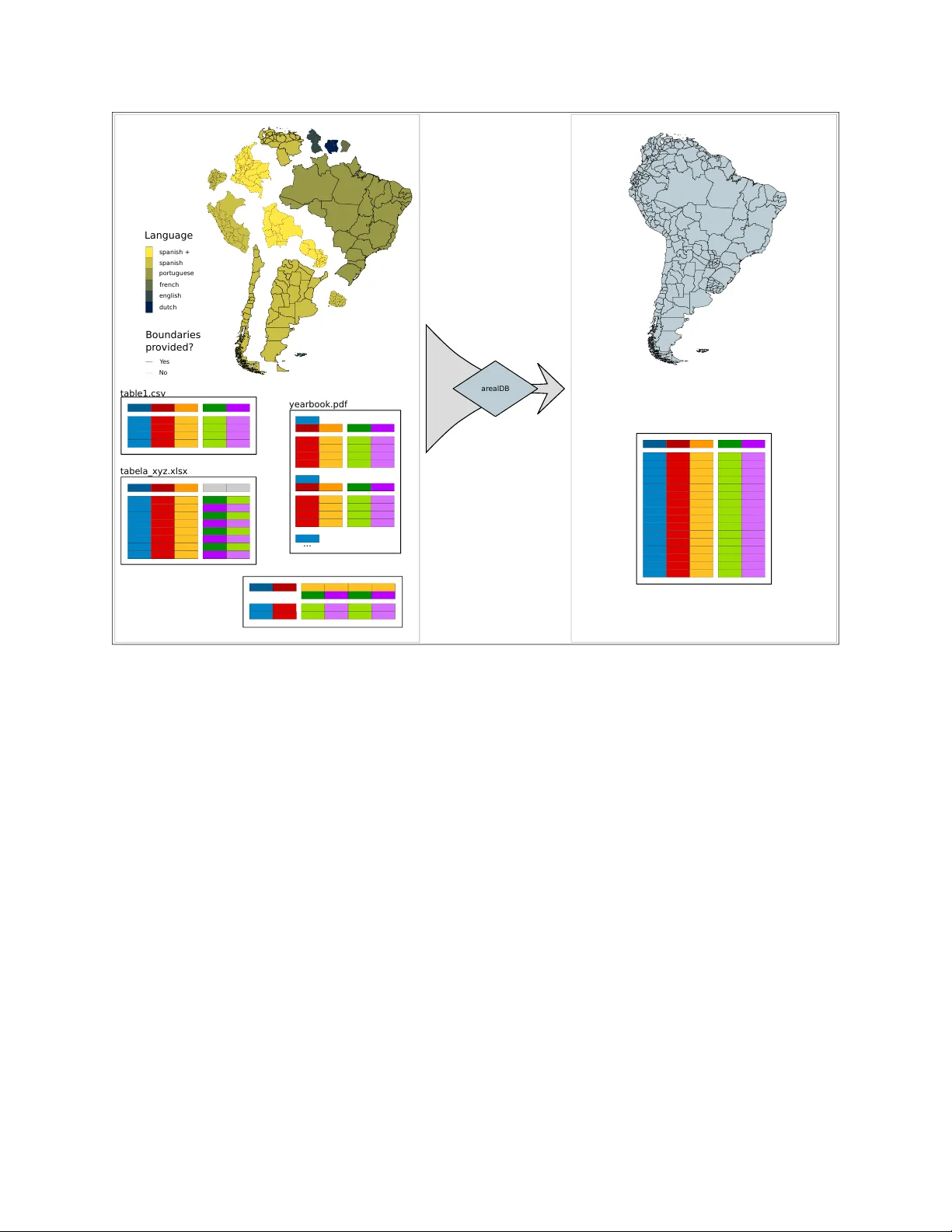
A P R E P R I N T - J U L Y 1 5 , 2 0 2 0 Harmonise and integrate heterogeneous areal data with the R package arealDB Steffen Ehrmann 1,* Ralf Seppelt 2,3 , Carsten Meyer 1,3,4* 1 German Centre for Integrati v e Biodi versity Research (iDi v) Halle-Jena-Leipzig, Deutscher Platz 5e, 04103 Leipzig, Germany 2 UFZ – Helmholtz Centre for En vironmental Research, Leipzig, Department Computational Landscape Ecology , Permoserstraße 15, 04318 Leipzig, Germany 3 Institute of Geosciences and Geography , Martin Luther Univ ersity Halle-W ittenber g, Halle (Saale), Germany 4 Institute of Biology , Leipzig Univ ersity , Leipzig, Germany * steffen.ehrmann@idiv .de, carsten.me yer@idiv .de A B S T R A C T Many rele v ant applications in the en vironmental and socioeconomic sciences use areal data, such as biodi versity checklists, agricultural statistics, or socioeconomic surveys. For applications that surpass the spatial, temporal or thematic scope of an y single data source, data must be integrated from se veral heterogeneous sources. Inconsistent concepts, definitions, or messy data tables mak e this a tedious and error-prone process. T o date, a dedicated tool to address these challenges is still lacking. Here, we introduce the R package arealDB that integrates heterogeneous areal data and associated geometries into a consistent database , in an easy-to-use workflow . It is useful for harmonising language and semantics of variables, relating data to geometries, and documenting metadata and prov enance. W e illustrate the functionality by integrating two disparate datasets (Brazil, USA) on the harvested area of soybean. arealDB promises quality-improv ements to do wnstream scientific, monitoring, and management applications b ut also substantial time-sa vings to database collation efforts. K eywords interoperability · census data · indicator data · polygon data · data warehouse · provenance documentation Software a v ailability arealDB is an R package that is a v ailable from CRAN via the function install.packages("arealDB") . This paper is based on version v0.3.6, which is installed via devtools::install_github("EhrmannS/arealDB@v0.3.6") . All programming was performed by the authors unless stated otherwise. 1 Introduction Areal data are an essential data type in man y socioeconomic applications, from visualising characteristics of human populations, to assessing trade statistics or documenting land ownership. They are increasingly used to analyse v arious en vironmental v ariables such as global biodi versity patterns. Areal data are an e veryday communication tool in ci vil society , where they play an important role as illustrati v e maps in news or education media. Generally , an y phenomenon at the lev el of finite spatial polygons (called geometries henceforth) is recorded as areal data , irrespective of the domain. Areal data are typically collated and curated by a di verse set of actors, from small and focused projects that b uild datasets around their particular observ ations, for example in nature conserv ation, to national statistical agencies or intergo vernmental or ganisations such as the W orld Bank Group 1 or the Food and Agriculture Organization 2 . The data are presented in formats, arrangements, languages and with definitions that are primarily adapted to a specific purpose, resulting in many distinct datasets that are by default not interoperable. Ho we ver , many important downstream applications and analyses surpass the spatial, temporal or thematic scope of any unique data source or organisation, and thus rely on combining data from multiple different sources (Otto et al. [2015]). 1 https://data.worldbank.or g/ 2 http://www .fao.org/faostat 1 A P R E P R I N T - J U L Y 1 5 , 2 0 2 0 Integrating areal data across man y sources comes with a large number of challenges (T ab . 1) that w ould, if not addressed, affect database consistency and potentially bias do wnstream analyses. For e xample, data tables that refer to the same areas must match one another , both spatially and lexically (Du et al. [2013]), for databases to be consistent. Besides, terms that emer ge from different languages or ontologies must correspond to one another , so that a v ariable that has different names in different source data does in fact match (De Giacomo et al. [2018]). Moreov er , alternati v e data that describe disputed areas or ha v e been recorded by different institutions should be ackno wledged to a v oid bias due to erroneous political assumptions, and final outputs should be appropriately documented (Henzen et al. [2013]). T able 1. List of issues, which have to be considered when b uilding a database of areal data from distinct sources. challenge class requir ed activity reproject geometries georeferencing harmonise spatial projection of distinct input geome- tries to be able to match them spatially match geometries and unit names georeferencing connect names of territorial units to the correct geome- tries territorial changes alternati ve data match areal data associated to territorial units that change through time data sources that disagree alternati ve data match areal data associated with the same territorial units provided by different data sources disputed areas alternati ve data identify data that belong to territorial units that are claimed by different authorities territorial unit names translation translate territorial unit names into a common language distinct concepts translation map variable names and v alues of categorical v ariables to standardised concepts disorganised messy data documentation arrange all data in the same format metadata documentation document dataset characteristics when input data are retrie ved from the source data prov enance documentation document the procedure by which the final data product was deri v ed Sev eral of the challenges in integrating areal data can be addressed indi vidually with specialised tools. For instance, a so-called ETL procedure (extract, transform, load) is typically used in data warehousing, where data from different sources are inte grated into a single database (Baumer [2017], Debroy et al. [2018]). Moreov er , geometries can be matched with GIS software such as QGIS, and ontologies that describe and relate distinct concepts can be created with the software Protégé (Horridge [2011]). Finally , data can be made av ailable via so-called Spatial Data Infrastructures (van den Brink et al. [2017]) and data values of the resulting database can be cleaned or validated with R-packages such as dataMaid (Petersen and Ekstrøm [2019]) . Howe ver , some specific challenges, such as to document input metadata or prov enance or to reshape messy data (W ickham [2014]) are typically solved in non-standardised w ays (if at all) via custom scripts or macros that are de veloped for indi vidual use-cases. Oftentimes, important steps of database management are ev en carried out manually , e.g., by comparing information visually and entering the data by hand into an Excel file. Notwithstanding the existence of many specialised tools, in practice, their application is not always tri vial and may require specific expert knowledge or e xpensi ve proprietary software (Debroy et al. [2018]). Moreover , none of the existing tools can address the full range of typical problems, so that combinations of independent tools are needed, which comes with further issues of interoperability of the specialised tools. This complexity increases resource and time requirements for a comprehensiv e workflo w , hindering successful implementation and thus scientific progress (Baumer [2017]). T o date, a coherent and easy-to-use solution for integrating areal data that considers a lar ge number of frequent issues and that is implemented in a robust and reproducible manner is still lacking. Here, we introduce the R software package arealDB to address the ov erall challenge of integrating heterogeneous areal data in an easy-to-use framework. The package offers a set of tools that are focused specifically on harmonisation and inte gration of areal data, thereby reducing complexity and increasing utility and confidence in data quality for downstream applications. arealDB automates complicated and error -prone procedures, such as reshaping data tables, semantic matching from v ocabularies or metadata and prov enance documentation, with only limited required user-input. Finally , it provides extensi v e unit testing, ensuring that all tools work as e xpected. W e ex emplify the full functionality of arealDB by integrating two e xample datasets on the harvested area of so ybean. The first dataset (Brazil) is pro vided in Portuguese language and accompanied by specific geometries, while the second 2 A P R E P R I N T - J U L Y 1 5 , 2 0 2 0 datasets (USA) is provided in our tar get language English and does not come with geometries b ut merely refers to the names of US counties. 3 A P R E P R I N T - J U L Y 1 5 , 2 0 2 0 2 Methods The R software package arealDB contains three groups of tools that reflect three stages of data management: (Fig. 1): • Stage 1 (Initialisation): Set up a database while gathering thematic metadata. • Stage 2 (Registration): Transform original data from downloaded files into standardised data formats and gather metadata on those files. • Stage 3 (Normalisation): Harmonise geometries and data tables based on the metadata collected at stage 2, and integrate them in a standardised database. T echnical documentation of any function that comes with this package can be retrie ved after installation, for e xample, via the command ?setPath for the function of that name. data table s Gazetteers GADM Setup I Registr atio n II Norm ali sati on III V oc abul aries D ar win C ore T a xonomies In v ent ories Schema descript ions Metadata Documentation Final harmonised database organised b y c ountr y Sourc es of areal data ... and man y more Sourc es of standar dised ... geometries/ shape fi les __.csv __.gpk g geometries data table s Figure 1. Flow-chart of the general workflow of data integration using arealDB . In stage 1, tables containing standardised terms for all v ariables of interest are read in to establish an ontological basis. In stage 2, data tables and geometries that hav e been do wnloaded from various data sources are re gistered. In stage 3, those files are harmonised and inte grated into the final database. The shown data sources, gazetteers, taxonomies and vocab ularies are an exemplary , non exhausti v e list of sources that can be handled with arealDB . 2.1 Project setup An areal database is started with the function setPath() , which creates the standardised directory structure in which the database is stored (Fig. 2a). All further operations within arealDB that rely on a path are then relati ve to this database directory . Any areal database typically contains a set of variables that identify the observed areal units, such as the unit names. Howe v er , it would also include other variables that identify the observed phenomenon, such as timesteps, socioeconomic groups of people, agricultural or other commodities or biological species. The function setVariables() is used to setup the v ariables that are used in a project to handle lexical translation and semantic harmonisation of the terms of those variables (Fig. 2b). It creates, by default, the skeleton of two files per variable and database, (1) an index table, which relates the v ariables’ terms to an ID and ancillary information and (2) a translation table, which relates terms in foreign languages and semantics to the tar get language/ontology . T o utilize index tables, an input table that contains term-ID pairs is indispensable and translation tables do not hav e to, but can be pro vided with standardised translations of the target v ariables, which can help impro ving consistency and data quality (Fig. 1). 4 A P R E P R I N T - J U L Y 1 5 , 2 0 2 0 Sources of such standardised tab ular information may be, for example, gazetteers such as GeoNames (GeoNames [2019]) or the ancillary data in the Global Administrativ e Areas database (GADM) (Hijmans [2019]), biological taxonomies such as The Plant List (The Plant List [2013]), W oRMS (Horton et al. [2019]) or the IUCN Red List (IUCN [2019]), or standardised ontologies, such as those offered by F A OST A T (F A O [2019]), the Darwin Core (W ieczorek et al. [2012]), the Humboldt Core (Guralnick et al. [2018]), or the Land Administration Domain Model(Lemmen et al. [2015]). (a) (b) to stage 2 Start DB setPath( ) setVaria bles() inv_tables.c sv inv_geometries.c sv inv_dataser ies.csv ID tables tran slation tables log stage1 stage3 adb_geometry incoming stage1 meta stage2 stage3 stage2 adb_tables incoming meta schem as Figure 2. Flow-chart of the project setup. (a) The function setPath() initiates the project by creating a directory structure in which the files are stored and by creating the inv entory tables for data-series, geometries and census tables. (b) The function setVariables() creates index and translation tables for all v ariables that should be handled in this project. 2.2 Data registration An important aspect to ensure the quality of an integrated database is prov enance documentation. This allows tracing errors that may show only in the final database to the specific source datasets or to a certain modification process. Documenting prov enance requires that the input state of a dataset, as well as procedural metadata that become available as a side-product in the ev olution from input to output data, be kno wn. Thus, the second stage in integrating data with arealDB is to create an inv entory of the rele vant files and to record metadata on the initial state of data, such as original file names, file locations, licenses and the arrangement of data tables (this process is called r e gistering in arealDB ). The arrangement of data tables is managed via the independent R-package tabshiftr (Ehrmann and Rümmler [2020]). Here, so-called schema descriptions are defined, where the table-specific arrangement is described by the position (columns and ro ws) of data components in the table, which is the basis for automatically reshaping the files in stage 3. arealDB thoroughly documents metadata on three kinds of information, data-series, geometries and data tables. Data- series are collections of data that are provided by the same source and which share more or less the same tabular arrangement and organisational logic. By documenting the data-series, one mostly documents information about a particular data provider and creates a tag that is common for input data that "belong together" and typically share a common structure. That information will eventually be documented in the three in v entory tables of the respecti v e names inv_dataseries.csv , inv_geometries.csv and inv_tables.csv . None of these in ventory tables e v er need to be modified by hand, as all information documented here is managed automatically . 5 A P R E P R I N T - J U L Y 1 5 , 2 0 2 0 A ne w data-series is re gistered with the function regDataseries() , before geometries and data tables, which are registered with the functions regGeometry() and regTable() (Fig. 3). The functions carry out the following operations: • check the arguments for valid v alues and consistenc y ,. • ov ersee that the indi vidual items are transformed to the tar get format with standard names and stored in the correct directory , • create IDs for all items and insert the provided metadata into the respectiv e in v entory tables. regDatas eries() regGeome try() original geometry (GADM) inv_dataser ies.csv regTable () original data ta ble fr om stage 1 to stage 3 (a) (b) (c) inv_geometries.c sv r egister ed geometry (GADM) inv_tables.c sv r egister ed data ta ble Figure 3. Flow-chart of the registration procedur e. (a) The function regDataseries() is used to document the various data-series (both, of data tables and geometries) that are provided by the data source. (b) The func- tion regGeometry() is then used to register all geometry files that ha ve been do wnloaded. (c) Finally , the func- tion regTable() is used to register all census tables that have been downloaded, and to relate the census tables to data-series and geometries. The re gistered files are stored in the folders "/adb_geometries/stage2" and "/adb_tables/stage2" . 2.3 Data normalisation The third and final step to integrate areal data consists of reshaping and harmonising the output of stage 2 (Fig. 4) and this process is called normalising in arealDB (Codd [1990]). This final step is crucial, since at stage 2, there is still no guarantee that names of territorial units in geometries are associated with those in data tables or that areal data are georeferenced, that variables are pro vided in the same language across several sources, or that data tables are provided in a compatible arrangement. Geometries are typically provided as shape or geopackage files, which ha v e already been optimised for interoperability , and where it is thus sufficient to kno w which columns in the attrib ute table contain names of the territorial units (see 6 A P R E P R I N T - J U L Y 1 5 , 2 0 2 0 regGeometry() ). The function normGeometry() builds harmonised geometry collections with regard to coordinate reference system, as well as semantically interoperable attribute tables. The ov erall procedure is detailed in Fig. A.1. There is no generally accepted way of recording data in tables so that these can be vastly more comple x or messy than geometries, and hence require schema descriptions. The schema descriptions that ha v e been recorded at stage 2 document accurate positions of variables held in data tables. The function normTable() utilises those schemas, in concert with the function tabshiftr::reor ganise() , to reshape the data into syntactically interoperable tables. It utilises, furthermore, the functions matchUnits() and matchVars() to harmonise labels of territorial units and the le v els of identifying variables to end up with semantically interoperable data tables. r egister ed geometry (GADM) r egister ed geometry (GADM) r egister ed geometry (GADM) fr om stage 2 normGeom etry() geometries gr ouped per nation data ta bles gr ouped per nation r egister ed data ta ble r egister ed data ta ble r egister ed data ta ble normTabl e() Figure 4. Flow-chart of the normalisation procedure . The function normGeometry() groups geometries per nation and creates the administrative hierar c hy ID (ahID) . The function normTable() reshapes the data tables into tidy format, calls matchUnits() to assign ahID to the areal data and groups the tables per nation. The normalised files are stored in the folders "/adb_geometries/stage3" and "adb_tables/stage3" 2.4 The administrative hierarchy Geometries in arealDB are assigned a unique ID for each territorial unit at each administrativ e le vel. This requires, first of all, an initial geometry dataset from which this administrative hierar chy ID (ahID) can be constructed, and which must thus include information on the hierarchical arrangement of the territorial units. At each administrativ e lev el a three-digit ID is assigned to the alphabetically sorted unit names. When descending into a lower le v el, that ID is restarted at 0 within each parent unit. For instance, T artu County in Estonia has the ahID 070013 , as Estonia is the 70th country (alphabetically) and T artu County the 13th county within Estonia. 2.5 T ranslating terms When handling data from sources that span lar ge spatial e xtents, these are lik ely only present in different languages. Howe v er , terms may be provided not only in different languages ( sensu stricto ), but also with distinct semantic meanings. For example, the concept of patch of land that is dominated by grassy ve getation and on which cattle graze , could be called "pasture" (British English), but also "rangeland" (American English), and is called "pastagem" in Portuguese. The language translation "pastagem <-> pasture" from Portuguese to English is functionally similar to the semantic translation "rangeland <-> pasture". Both examples are cases of many-to-one translations because terms in different languages ( sensu lato ) refer to the same term in the target language. Additionally , in a particular dataset, 7 A P R E P R I N T - J U L Y 1 5 , 2 0 2 0 the term "pasture" might refer to anything from atificially maintained gr assland manag ed for livestock gr azing to natural grassland (i.e., with or without liv estock). Ideally , these different meanings will become evident from a v ailable metadata. In arealDB , an indi vidual term is allo wed to refer to different concepts, depending on where it originates, which constitutes a one-to-many semantic translation. Many-to-one translations are handled quite straightforwardly , in that the target v alue is repeated in the column target for each translation and terms that refer to it are recorded in the column origin (T ab . 2). One-to-many translations are provided, in the column source , either with geoID or tabID , depending on whether the terms originate from geometries or tables, and in ID with the respecti ve ID. T able 2. A translation table that includes (a) many-to-one translations (lines 1 and 2) and a case of one-to-many translations (line 3), as well as (b) language (line 1) and semantic (lines 2 and 3) translations of the term ’pasture’. origin target source ID notes pastagem pasture rangeland pasture pasture grassland tabID 3 ... The function translateTerms() manages all translations by comparing ne w terms individually and explicitly with the translation tables that have been created in stage 1. The user is pro vided with an interface that suggests a range of terms pre-selected from the translation table via approximate string matching (fuzzy matching). The missing translations then hav e to be provided by the user , so that the ne w terms can finally be compared against the look-up section of the translation table to check for consistent translations. 3 Results W e have tested the described functionalities on sev eral dozen agricultural and forestry census datasets from most countries of the American continent. These data represent many of the challenges outlined in T ab. 1, including different table arrangements of the areal data, dissimilar v ariables provided in different languages and associations to geometries, if they were pro vided at all, in distinct spatial projections. In Appendix A, we exemplarily sho wcase the inte gration of data on the soybean harv ested area for Brazil and the US. Do wnstream applications, such as maps of the spatial patterns (Fig. 5 and Appendix B) or e xplorati ve analysis, can profit from the relativ e ease of accessing all data in a database that has been built with arealDB at once. 400500 300375 200250 10012 5 0 Figure 5. Choropleth maps of the final, integrated database . The maps ha ve been created with the simple code snippet that is shown in Appendix B. The standardised geometries and data tables were read in with a loop through all countries of interest and the maps were created with another loop through the years of interest to plot the data via the R-package geometr (Ehrmann [2019]). 8 A P R E P R I N T - J U L Y 1 5 , 2 0 2 0 The schema descriptions for each input dataset are central to this workflo w . They record the type of each variable, the locationin a spreadsheet ( row , col ) at which the v ariable is and other metadata that are relev ant to reshape the table. At stage 2, the Brazilian dataset is organised in a systematic way , ho we ver the arrangement is rather complicated (Listing 1). First of all, the spreadsheet contains a metadata header in the first three rows so that the origin of the table is at the fourth ro w in the first column. The values of the identifying v ariables "years" and "commodities" and the target v ariable "harvested" are stored in the same columns. Moreover , states ( al2 ) and municipalities ( al3 ) are combined in the first column, so that this column has to be split. The names of the states are abbreviated, requiring translation to correct names (e.g., "R O <-> Rondônia"). l i b r a r y ( r e a d r ) # i n p u t a n d s c h e m a f o r B r a z i l r e a d _ c s v ( f i l e = p a s t e 0 ( d b P a t h , " / a d b _ t a b l e s / s t a g e 2 / p r o c e s s e d / b r a _ 3 _ s o y _ 2 0 0 0 _ 2 0 1 8 _ i b g e . c s v " ) , c o l _ n a m e s = F A L S E ) # > # A t i b b l e : 5 , 5 6 9 x 2 0 # > X 1 X 2 X 3 X 4 X 5 X 6 X 7 X 8 X 9 X 1 0 # > < c h r > < c h r > < c h r > < c h r > < c h r > < c h r > < c h r > < c h r > < c h r > < c h r > # > 1 T a b e l N A N A N A N A N A N A N A N A N A # > 2 V a r i a N A N A N A N A N A N A N A N A N A # > 3 M u n i c A n o x N A N A N A N A N A N A N A N A # > 4 N A 2 0 0 0 2 0 0 1 2 0 0 2 2 0 0 3 2 0 0 4 2 0 0 5 2 0 0 6 2 0 0 7 2 0 0 8 # > 5 N A S o j a S o j a S o j a S o j a S o j a S o j a S o j a S o j a S o j a # > 6 A l t a - - - - 1 0 0 - - - - # > 7 A r i q u - - 4 5 0 - - - 5 0 - - # > 8 C a b i x 2 0 0 4 8 6 6 0 0 1 5 0 0 1 5 0 0 5 3 7 0 7 5 0 0 6 0 0 0 7 0 0 0 # > 9 C a c o a - - - - - - - - - # > 1 0 C e r e j 2 7 0 0 3 3 5 3 3 4 0 0 4 5 1 6 7 1 8 4 8 0 0 0 1 8 0 0 0 1 6 2 0 0 1 8 0 0 0 # > # w i t h 5 , 5 5 9 m o r e r o w s , a n d 1 0 m o r e v a r i a b l e s : X 1 1 < c h r > , # > # X 1 2 < c h r > , X 1 3 < c h r > , X 1 4 < c h r > , X 1 5 < c h r > , X 1 6 < c h r > , # > # X 1 7 < c h r > , X 1 8 < c h r > , X 1 9 < c h r > , X 2 0 < c h r > r e a d _ r d s ( p a t h = p a s t e 0 ( d b P a t h , " / a d b _ t a b l e s / m e t a / s c h e m a s / s c h e m a _ 1 . r d s " ) ) # > 1 c l u s t e r # > o r i g i n : 4 | 1 ( t o p | l e f t ) # > # > v a r i a b l e t y p e r o w c o l r e l d i s t # > - - - - - - - - - - - - - - - - - - - - - - - - - - - - - - - - - - - - - - - - - - - # > a l 2 i d 1 F F # > a l 3 i d 1 F F # > y e a r i d 4 2 : 2 0 F F # > c o m m o d i t i e s i d 5 2 : 2 0 F F # > h a r v e s t e d m e a s u r e d 2 : 2 0 F F Listing 1. Schema description of the Brazilian dataset The US dataset, on the other hand, is already "tidy" at stage 2, i.e., all v ariables are recorded in individual columns that simply hav e to be selected, and no lexical or ontological translations are required (Listing 2). r e a d _ c s v ( f i l e = p a s t e 0 ( d b P a t h , " / a d b _ t a b l e s / s t a g e 2 / p r o c e s s e d / u s a _ 3 _ s o y _ 2 0 0 0 _ 2 0 1 8 _ u s d a . c s v " ) , c o l _ n a m e s = F A L S E ) # > # A t i b b l e : 3 0 , 1 4 3 x 2 1 # > X 1 X 2 X 3 X 4 X 5 X 6 X 7 X 8 X 9 X 1 0 # > < c h r > < c h r > < c h r > < c h r > < c h r > < c h r > < c h r > < c h r > < c h r > < c h r > # > 1 P r o g r Y e a r P e r i o d W e e k G e o S t a t e S t a t A g D A g D C o u n # > 2 S U R V E Y 2 0 1 8 Y E A R N A C O U N A L A B 1 B L A C 4 0 D A L L # > 3 S U R V E Y 2 0 1 8 Y E A R N A C O U N A L A B 1 B L A C 4 0 E L M O # > 4 S U R V E Y 2 0 1 8 Y E A R N A C O U N A L A B 1 B L A C 4 0 O T H E # > 5 S U R V E Y 2 0 1 8 Y E A R N A C O U N A L A B 1 B L A C 4 0 P E R R Y # > 6 S U R V E Y 2 0 1 8 Y E A R N A C O U N A L A B 1 B L A C 4 0 S U M T # > 7 S U R V E Y 2 0 1 8 Y E A R N A C O U N A L A B 1 C O A S 5 0 B A L D # > 8 S U R V E Y 2 0 1 8 Y E A R N A C O U N A L A B 1 C O A S 5 0 O T H E # > 9 S U R V E Y 2 0 1 8 Y E A R N A C O U N A L A B 1 M O U N 2 0 B L O U # > 1 0 S U R V E Y 2 0 1 8 Y E A R N A C O U N A L A B 1 M O U N 2 0 C H E R # > # w i t h 3 0 , 1 3 3 m o r e r o w s , a n d 1 1 m o r e v a r i a b l e s : X 1 1 < c h r > , # > # X 1 2 < c h r > , X 1 3 < c h r > , X 1 4 < c h r > , X 1 5 < c h r > , X 1 6 < c h r > , # > # X 1 7 < c h r > , X 1 8 < c h r > , X 1 9 < c h r > , X 2 0 < c h r > , X 2 1 < c h r > 9 A P R E P R I N T - J U L Y 1 5 , 2 0 2 0 r e a d _ r d s ( p a t h = p a s t e 0 ( d b P a t h , " / a d b _ t a b l e s / m e t a / s c h e m a s / s c h e m a _ 2 . r d s " ) ) # > 1 c l u s t e r ( w h o l e s p r e a d s h e e t ) # > # > v a r i a b l e t y p e r o w c o l r e l d i s t # > - - - - - - - - - - - - - - - - - - - - - - - - - - - - - - - - - - - - - - - - - - # > a l 2 i d 6 F F # > a l 3 i d 1 0 F F # > y e a r i d 2 F F # > c o m m o d i t i e s i d 1 6 F F # > h a r v e s t e d m e a s u r e d 2 0 F F Listing 2. Schema description of the US dataset After normalising (at stage 3), both tables share the same arrangement, where e very information is encoded by IDs that point either to metadata ( tabID , geoID ), territorial units ( ahID ), or to commodities ( faoID ). r e a d _ c s v ( f i l e = p a s t e 0 ( d b P a t h , " / a d b _ t a b l e s / s t a g e 3 / b r a z i l . c s v " ) , c o l _ t y p e s = " i i i i i d i " ) % > % s u m m a r y ( ) # > i d t a b I D g e o I D a h I D # > M i n . : 1 M i n . : 1 M i n . : 5 M i n . : 3 2 0 0 1 0 0 1 # > 1 s t Q u . : 2 4 6 4 8 1 s t Q u . : 1 1 s t Q u . : 5 1 s t Q u . : 3 2 0 1 1 0 2 9 # > M e d i a n : 4 9 2 9 6 M e d i a n : 1 M e d i a n : 5 M e d i a n : 3 2 0 1 5 1 9 7 # > M e a n : 4 9 2 9 6 M e a n : 1 M e a n : 5 M e a n : 3 2 0 1 5 7 9 3 # > 3 r d Q u . : 7 3 9 4 4 3 r d Q u . : 1 3 r d Q u . : 5 3 r d Q u . : 3 2 0 2 1 3 0 6 # > M a x . : 9 8 5 9 1 M a x . : 1 M a x . : 5 M a x . : 3 2 0 2 7 1 3 7 # > # > y e a r h a r v e s t e d f a o I D # > M i n . : 2 0 0 0 M i n . : 0 M i n . : 2 3 6 # > 1 s t Q u . : 2 0 0 4 1 s t Q u . : 4 6 0 1 s t Q u . : 2 3 6 # > M e d i a n : 2 0 0 9 M e d i a n : 2 9 5 0 M e d i a n : 2 3 6 # > M e a n : 2 0 0 9 M e a n : 1 2 3 8 8 M e a n : 2 3 6 # > 3 r d Q u . : 2 0 1 4 3 r d Q u . : 1 1 5 0 0 3 r d Q u . : 2 3 6 # > M a x . : 2 0 1 8 M a x . : 4 1 1 2 2 4 M a x . : 2 3 6 # > N A ’ s : 6 5 5 2 9 r e a d _ c s v ( f i l e = p a s t e 0 ( d b P a t h , " / a d b _ t a b l e s / s t a g e 3 / u n i t e d s t a t e s o f a m e r i c a . c s v " ) , c o l _ t y p e s = " i i i i i d i " ) % > % s u m m a r y ( ) # > i d t a b I D g e o I D a h I D # > M i n . : 1 M i n . : 2 M i n . : 3 M i n . : 2 3 8 0 0 1 0 0 1 # > 1 s t Q u . : 6 8 7 1 1 s t Q u . : 2 1 s t Q u . : 3 1 s t Q u . : 2 3 8 0 1 6 0 7 4 # > M e d i a n : 1 3 7 4 0 M e d i a n : 2 M e d i a n : 3 M e d i a n : 2 3 8 0 2 5 0 5 4 # > M e a n : 1 3 7 4 0 M e a n : 2 M e a n : 3 M e a n : 2 3 8 0 2 6 6 4 7 # > 3 r d Q u . : 2 0 6 1 0 3 r d Q u . : 2 3 r d Q u . : 3 3 r d Q u . : 2 3 8 0 3 6 0 6 5 # > M a x . : 2 7 4 8 0 M a x . : 2 M a x . : 3 M a x . : 2 3 8 0 5 0 0 7 4 # > y e a r h a r v e s t e d f a o I D # > M i n . : 2 0 0 0 M i n . : 4 0 . 4 7 M i n . : 2 3 6 # > 1 s t Q u . : 2 0 0 4 1 s t Q u . : 2 9 5 4 . 2 1 1 s t Q u . : 2 3 6 # > M e d i a n : 2 0 0 8 M e d i a n : 1 2 7 8 8 . 0 7 M e d i a n : 2 3 6 # > M e a n : 2 0 0 9 M e a n : 2 0 3 0 2 . 9 0 M e a n : 2 3 6 # > 3 r d Q u . : 2 0 1 3 3 r d Q u . : 3 3 1 0 8 . 3 4 3 r d Q u . : 2 3 6 # > M a x . : 2 0 1 8 M a x . : 2 1 8 1 2 5 . 5 6 M a x . : 2 3 6 Listing 3. Summary of the core table of the harmonised and integrated database 4 Discussion The present R package arealDB provides so far missing software for harmonising and integrating areal data across multiple heterogeneous sources into a single, consistent database (Fig. 6). By guiding users through the three stages ’project setup’, ’ data registration’ and ’ data normalisation’ , embedded into a collaborati ve and transparent software en vironment (Lo wndes et al. [2017]), arealDB substantially impro ves the speed, scientific accuracy , and reproducibility of integrating areal data . 10 A P R E P R I N T - J U L Y 1 5 , 2 0 2 0 ar ealDB Language Boundaries pr ovided? Y es No spanish + spanish portugu ese fr ench dutch english table1.cs v tabela_xyz.xlsx ... yearbook.pdf Figure 6. Schematic overview of the purpose of arealDB . Both, data tables that are disor ganised and messy and that are based on different languages and concepts, as well as distinctly org anised geometric datasets are harmonised and integrated into one consistent database. Lacking such a tool, many data integrators ha v e thus far gone through a highly time-consuming and error-prone process of opening individual input datasets in Excel, translating variables "by hand", and reshaping tables by copying relev ant data from one spreadsheet into another , typically without any prov enance documentation. More sophisticated workflo ws based on adv anced tools, such as lookup and pi vot tables or programmable statistical/data management tools often require custom-scripted solutions for the different, heterogeneous input data-sets. arealDB , by contrast, merely requires that users document metadata, provide translation tables and specify a schema description for each dataset. 4.1 Handling geometries Using arealDB , each indi vidual areal data table may be linked to a different geometry dataset. This helps to a v oid political and other assumptions where more than one source of areal data exists for territorial units, for example in cases of disputed areas or administrati ve changes. Data that refer to such disparate geometry sources can coexist in a database without biasing downstream analyses that are sensiti ve to the areas of measurement units (e.g., when estimating ecological scaling relationships from species checklists; (Kreft and Jetz [2007]; K eil and Chase [2019]). Where such considerations are not an issue, datasets may be linked to standardised geometries, such as GADM (Hijmans [2019]). Currently , arealDB matches areal data via an internal assessment of the geographical overlap of geometries (using the R package sf (Pebesma [2018]); see flowchart in Appendix C). This procedure could be further refined by additionally incorporating functions that can automatically detect and handle temporal changes of territorial units (Bernard et al. [2018]). Howe ver , as all ra w input geometries are retained in the final database, more sophisticated procedures for matching recorded geometries may be applied alongside arealDB ’ s own functions. Another common challenge in matching territorial units lies in names that are shared by multiple territorial units located in different nations and at different administrati v e le vels. For e xample, the term ’Santa Cruz’ may refer to city districts, 11 A P R E P R I N T - J U L Y 1 5 , 2 0 2 0 municipalities, departments, or other units in over twenty different nations. arealDB addresses this issue by matching territorial unit names to geometries hierarchically . 4.2 Documenting metadata Even arealDB is still prone to some human error , mostly related to correctly reading in the required files and information. arealDB ’ s syst em of unique IDs ensures that all data v alues can be linked to metadata on their input tables, associated geometries, and original data sources. Hence, inconsistencies that may still exist in an output database are fully traceable, due to the metadata collected while collating the database (Henzen et al. [2013]). Moreov er , the relational setup of the resulting database allows that database management software can retriev e metadata on all harmonised datasets (e.g., the recorded number of entities or observations, or value ranges) and make those and other metadata av ailable also to other tools and en vironments. 4.3 Interoperability arealDB was primarily designed for the purpose of integrating heterogeneous areal data within a gi v en knowledge domain. Howe ver , by storing all v ariables in the same data structure, the tools provided here enable areal databases that are syntactically interoperable across domains. The areal data in each and every output table of arealDB hav e a v alue of ahID (Code-Listing 3) that is by default alw ays deri ved from the same spatial basis, the GADM dataset. Merely areal data for which ahID was derived from specific non-GADM geometries may deviate from a common list of ahID values. This means that areal databases from se veral distinct domains (for instance, human health and biodi versity) that ha v e all been built with the same geometries dataset can simply be joined via ahID to combine information on the distinct topics within a consistent database and facilitate interdisciplinary applications (Otto et al. [2015]). While arealDB enables such data integration technically , the endeavour of actually integrating databases across knowledge domains in a meaningful way hinges crucially on adv ances in ontological standardisation to come up with concepts that are valid simultaneously across kno wledge domains (v an den Brink et al. [2017]). 5 Conclusions arealDB provides a range of tools that standardise the process of inte grating heterogeneous areal data sources into a single, harmonised database, removing hurdles that come with high resource and time requirements. It enables users that may lack the necessary background knowledge to address the majority of the anticipated issues in setting up a coherent workflo w of data integration. This helps in homogenising data collection methodologies, which is urgently needed to tackle data management strategies that are able to deal with v ast amounts of heterogeneous data (Otto et al. [2015]). The tools presented here allow to process any areal data, such as socioeconomic census and surv ey data, ecological checklist data, data on infectious diseases, (sub-)national indicator data, cadastral parcel data, and man y more. arealDB lowers the effort to surpass barriers of the spatial, temporal or thematic scope of single data sources. This can enable many e xciting and easy to set-up applications at the pan-re gional and global scale, supporting data-inte gration needs across application domains and progressing tow ards multiple Sustainable De velopment Goals. 6 Acknowledgements CM ackno wledges funding by the V olkswagen F oundation via a Freigeist Fello wship. SE ackno wledges funding by iDiv via the Fle xpool mechanism (FZT -118, DFG). 7 A ppendix • Appendix A: Replication Script • Appendix B: Downstream Application • Appendix C: Normalise Geometries References Benjamin S Baumer . A grammar for reproducible and painless extract-transform-load operations on medium data. Journal of Computational and Graphical Statistics , 28(2):256–264, 2017. doi: 10.1080/10618600.2018.1512867. 12 A P R E P R I N T - J U L Y 1 5 , 2 0 2 0 Camille Bernard, Christine Plumejeaud-Perreau, Marlène V illano v a-Oliv er , Jérôme Gensel, and Hy Dao. An ontology- based algorithm for managing the e volution of multi-level territorial partitions. In Pr oceedings of the 26th A CM SIGSP ATIAL International Confer ence on Advances in Geographic Information Systems , pages 456–459. A CM, 2018. doi: 10.1145/3274895.3274944. EF Codd. The Relational Model for Database Management: V ersion 2 . Addison-W esley Longman Publishing Co., Inc., Boston, MA, USA, 1990. ISBN 0-201-14192-2. Giuseppe De Giacomo, Domenico Lembo, Maurizio Lenzerini, Antonella Poggi, and Riccardo Rosati. Using ontologies for semantic data integration. In A Comprehensive Guide Thr ough the Italian Database Researc h Over the Last 25 Y ears , pages 187–202. Springer , 05 2018. ISBN 978-3-319-61892-0. doi: 10.1007/978- 3- 319- 61893- 7_11. V idroha Debroy , Lance Brimble, and Matt Y ost. Newtl: engineering an extract, transform, load (etl) softw are system for business on a very lar ge scale. In Pr oceedings of the 33r d Annual ACM Symposium on Applied Computing , pages 1568–1575. A CM, 2018. Heshan Du, Natasha Alechina, Mik e Jackson, and Glen Hart. Matching formal and informal geospatial ontolo- gies. In Geogr aphic information science at the heart of Eur ope , pages 155–171. Springer, 2013. doi: 10.1007/ 978- 3- 319- 00615- 4_9. URL https://link.springer.com/chapter/10.1007/978- 3- 319- 00615- 4_9 . Steffen Ehrmann. geometr: Generate and Modify Interoper able Geometric Shapes , 2019. URL https://github. com/EhrmannS/geometr . R package version 0.2.2. Steffen Ehrmann and Arne Rümmler . r ectifyr: Reshape disor ganised messy tables , 2020. URL https://gitlab. com/luckinet/software/rectifyr . R package version 0.1.2. F A O. Faostat, 2019. URL http://www.fao.org/faostat . GeoNames. Geonames, 2019. URL http://www.geonames.org . Robert Guralnick, Ramona W alls, and W alter Jetz. Humboldt core–toward a standardized capture of biological in v entories for biodi versity monitoring, modeling and assessment. Ecography , 41(5):713–725, 2018. URL https: //onlinelibrary.wiley.com/doi/full/10.1111/ecog.02942 . Christin Henzen, Stephan Mäs, and Lars Bernard. Provenance information in geodata infrastructures. In Geographic Information Science at the Heart of Eur ope , volume 2013, pages 133–151. Springer International Publishing, 05 2013. ISBN 978-3-319-00615-4. doi: 10.1007/978- 3- 319- 00615- 4_8. URL https://doi.org/10.1007/ 978- 3- 319- 00615- 4_8 . Robert J Hijmans. Global administrative areas, 2019. URL www.gadm.org . M Horridge. A practical guide to building o wl ontologies using protégé 4 and co-ode tools edition 1.3. retrieved march 10, 2013, 2011. T . Horton, A. Kroh, S. Ah yong, N. Bailly , C.B. Bo yko, S.N. Brandão, S. Gofas, J.N.A. Hooper, F . Hernandez, O. Holo- vacho v , J. Mees, T .N. Molodtsov a, G. Paulay , W . Decock, S. Deke yzer , T . Lanssens, L. V andepitte, B. V anhoorne, K. V erfaille, R. Adlard, P . Adriaens, S. Agatha, K.J. Ahn, N. Akkari, B. Alvarez, G. Anderson, M.V . Angel, C. Arango, T . Artois, S. Atkinson, R. Bank, A. Barber, J.P . Barbosa, I. Bartsch, D. Bellan-Santini, J. Bernot, A. Berta, T .N. Bezerra, R. Bieler , S. Blanco, I. Blasco-Costa, M. Blaze wicz, P . Bock, R. Böttger-Schnack, P . Bouchet, N. Boury- Esnault, G. Boxshall, R. Bray , B. Breure, N.L. Bruce, S. Cairns, P . Cárdenas, E. Carstens, B.K. Chan, T .Y . Chan, L. Cheng, M. Churchill, C.O. Coleman, A.G. Collins, L. Corbari, R. Cordeiro, A. Cornils, M. Coste, M.J. Costello, K.A. Crandall, F . Cremonte, T . Cribb, S. Cutmore, F . Dahdouh-Guebas, M. Daly , M. Daneliya, J.C. Dauvin, P . Davie, C. De Broyer , S. De Grav e, V . de Mazancourt, N.J. de V oogd, P . Decker , W . Decraemer , D. Defaye, J.L. d’Hondt, S. Dippenaar , M. Dohrmann, J. Dolan, D. Domning, R. Do wney , L. Ector, U. Eisendle-Flöckner , M. Eitel, S.C.d. Encarnação, H. Enghoff, J. Epler , C. Ewers-Saucedo, M. F aber , S. Feist, D. Figueroa, J. Finn, C. Fišer , E. Fordyce, W . F oster , J.H. Frank, C. Fransen, H. Furuya, H. Galea, O. Garcia-Alvarez, R. Garic, R. Gasca, S. Gaviria-Melo, S. Gerken, D. Gibson, R. Gibson, J. Gil, A. Gittenberger , C. Glasby , A. Glo ver , S.E. Gómez-Noguera, D. González- Solís, D. Gordon, M. Grabowski, C. Gravili, J.M.. Guerra-García, R. Guidetti, M.D. Guiry , K.A. Hadfield, E. Hajdu, J. Hallermann, B.W . Hayw ard, E. Hendrycks, D. Herbert, A. Herrera Bachiller , J.s. Ho, M. Hodda, J. Høeg, B. Hoek- sema, R. Houart, L. Hughes, M. Hyžný, L.F .M. Iniesta, T . Iseto, S. Iv anenk o, M. Iw ataki, R. Janssen, G. Jarms, D. Jaume, K. Jazdzewski, C.D. Jersabek, P . Jó ´ zwiak, A. Kabat, Y . Kantor , I. Karanovic, B. Karthick, Y .H. Kim, R. King, P .M. Kirk, M. Klautau, J.P . K ociolek, F . Köhler, J. K olb, A. K oto v , A. Kremenetskaia, R.M. Kristensen, M. Kulik ovskiy , S. Kullander , G. Lambert, D. Lazarus, F . Le Coze, S. LeCroy , D. Leduc, E.J. Lefko witz, R. Lemaitre, Y . Liu, A.N. Lörz, J. Lowry , T . Ludwig, N. Lundholm, E. Macpherson, L. Madin, C. Mah, B. Mamo, T . Mamos, R. Manconi, G. Mapstone, P .E. Marek, B. Marshall, D.J. Marshall, P . Martin, R. Mast, C. McF adden, S.J. McInnes, T . Meidla, K. Meland, K.L. Merrin, C. Messing, D. Miljutin, C. Mills, Ø. Moestrup, V . Mokievsky , F . Monniot, R. Mooi, A.C. Morandini, R. Moreira da Rocha, F . Moretzsohn, C. Morrow , J. Mortelmans, J. Mortimer , L. Musco, T .A. Neubauer , E. Neubert, B. Neuhaus, P . Ng, A.D. Nguyen, C. Nielsen, T . Nishikawa, J. Norenbur g, T . O’Hara, 13 A P R E P R I N T - J U L Y 1 5 , 2 0 2 0 D. Opresko, M. Osa wa, H.J. Osigus, Y . Ota, B. Páll-Gergely , D. Patterson, H. Paxton, R. Peña-Santiago, V . Perrier , W . Perrin, I. Petrescu, B. Picton, J.F . Pilger , A.B. Pisera, D. Polhemus, G.C. Poore, M. Potapo va, P . Pugh, G. Read, M. Reich, J.D. Reimer , H. Reip, M. Reuscher , J.W . Reynolds, I. Richling, F . Rimet, P . Ríos, M. Rius, D.C. Rogers, G. Rosenberg, K. Rützler , K. Sabbe, J. Saiz-Salinas, S. Sala, S. Santagata, S. Santos, E. Sar , A. Satoh, T . Saucède, H. Schatz, B. Schierwater , A. Schmidt-Rhaesa, S. Schneider, C. Schönberg, P . Schuchert, A.R. Senna, C. Serejo, S. Shaik, S. Shamsi, J. Sharma, W .A. Shear , N. Shenkar , A. Shinn, M. Short, J. Sicinski, P . Sierwald, E. Simmons, F . Sinniger , D. Si v ell, B. Sk et, H. Smit, N. Smit, N. Smol, J.F .. Souza-Filho, J. Spelda, W . Sterrer , E. Stienen, P . Stoev , S. Stöhr , M. Strand, E. Suárez-Morales, M. Summers, L. Suppan, C. Suttle, B.J. Swalla, S. T aiti, M. T anaka, A.H. T andberg, D. T ang, M. T asker , J. T aylor , J. T aylor, A. Tchesunov , H. ten Hov e, J.J. ter Poorten, J.D. Thomas, E.V . Thuesen, M. Thurston, B. Thuy , J.T . Timi, T . T imm, A. T odaro, X. T uron, S. T yler, P . Uetz, J. Uribe-P alomino, S. Ute vsky , J. V acelet, D. V achard, W . V ader , R. Väinölä, B. V an de V ijv er , S.E. v an der Meij, T . van Haaren, R.W . van Soest, A. V anreusel, V . V eneke y , M. V inarski, R. V onk, C. V os, G. W alker-Smith, T .C. W alter, L. W atling, M. W ayland, T . W esener , C.E. W etzel, C. Whipps, K. White, U. W ieneke, D.M. W illiams, G. Wil liams, R. W ilson, A. W itko wski, J. W itkowski, N. W yatt, C. W ylezich, K. Xu, J. Zanol, W . Zeidler , and Z. Zhao. W orld register of ma- rine species (worms). = http://www .marinespecies.org, 2019. URL http://www.marinespecies.org . Accessed: 2019-09-11. IUCN. The iucn red list of threatened species, 2019. URL http://www.iucnredlist.org . V ersion 2019-2. Petr Keil and Jonathan M Chase. Global patterns and driv ers of tree di versity inte grated across a continuum of spatial grains. Nature ecology & evolution , 3(3):390, 2019. doi: 10.1038/s41559- 019- 0799- 0. Holger Kreft and W alter Jetz. Global patterns and determinants of v ascular plant di v ersity . Pr oceedings of the National Academy of Sciences , 2007. doi: 10.1073/pnas.0608361104. URL https://www.pnas.org/content/104/14/ 5925 . Christiaan Lemmen, Peter V an Oosterom, and Rohan Bennett. The land administration domain model. Land use policy , 49:535–545, 2015. doi: 10.1016/j.landusepol.2015.01.014. URL https://www.sciencedirect.com/science/ article/pii/S0264837715000174?via%3Dihub . Julia S Ste wart Lo wndes, Benjamin D Best, Courtne y Scarborough, Jamie C Afflerbach, Melanie R Frazier , Casey C O’Hara, Ning Jiang, and Benjamin S Halpern. Our path to better science in less time using open data science tools. Natur e ecology & evolution , 1(6):1–7, 2017. doi: 10.1038/s41559- 017- 0160. Ilona M Otto, Anne Bie wald, Dim Coumou, Georg Feulner , Claudia Köhler , Thomas Nocke, Anders Blok, Albert Gröber , Sabine Selchow , David T yfield, et al. Socio-economic data for global en vironmental change research. Natur e Climate Change , 5(6):503, 2015. doi: 10.1038/nclimate2593. URL https://www.nature.com/articles/ nclimate2593.pdf . Edzer Pebesma. Simple Features for R: Standardized Support for Spatial V ector Data. The R Journal , 10(1):439–446, 2018. doi: 10.32614/RJ- 2018- 009. URL https://doi.org/10.32614/RJ- 2018- 009 . Anne Helby Petersen and Claus Thorn Ekstrøm. datamaid: Y our assistant for documenting supervised data quality screening in r . Journal of Statistical Software , 90(1):1–38, 2019. The Plant List. The plant list, 2013. URL http://www.theplantlist.org/ . V ersion 1.1. Linda van den Brink, Paul Janssen, W ilko Quak, and Jantien Stoter . T ow ards a high lev el of semantic harmonisation in the geospatial domain. Computers, Envir onment and Urban Systems , 62:233–242, 2017. doi: 10.1016/j.compen vurbsys. 2016.12.002. Hadley W ickham. Tidy data. Journal of Statistical Software , 59(10):1–23, 2014. doi: 10.18637/jss.v059.i10. URL https://www.jstatsoft.org/article/view/v059i10 . John W ieczorek, Da vid Bloom, Robert Guralnick, Stan Blum, Markus Döring, Renato Gio vanni, T im Robertson, and David V ieglais. Darwin core: an evolving community-de v eloped biodi versity data standard. PloS One , 7(1):e29715, 2012. doi: 10.1371/journal.pone.0029715. URL https://journals.plos.org/plosone/article/file?id= 10.1371/journal.pone.0029715&type=printable . 14