Robust delay-dependent LPV output-feedback blood pressure control with real-time Bayesian estimation

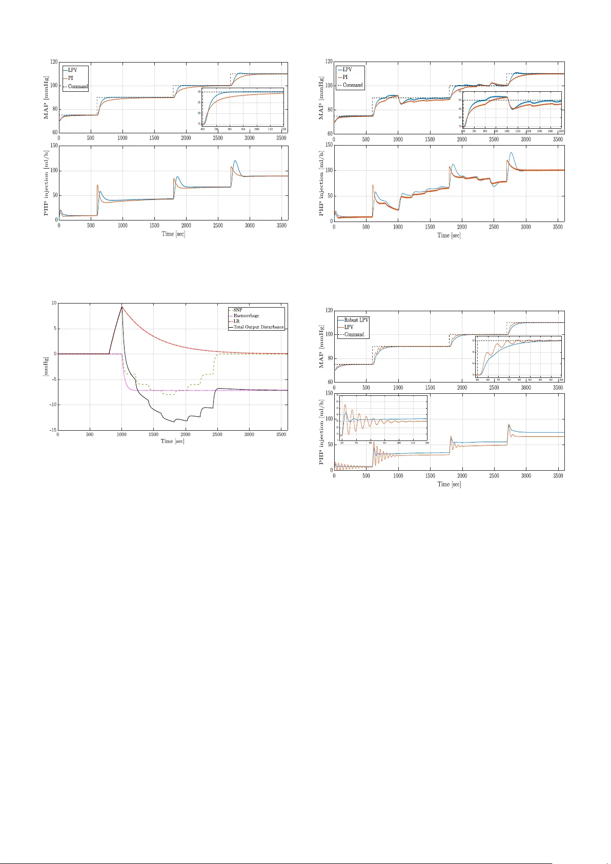
This paper is a preprint of a paper submitted to IET Control Theor y & Applications Rob ust dela y-dependent LPV output-feedbac k b lood pressure contr ol with real-time Ba yesian estimation ISSN 1751-8644 doi: 0000000000 www .ietdl.org S. T asoujian S. Salav ati M. F ranchek K. Gr igoriadis Depar tment of Mechanical Engineer ing, University of Houston, Houston, TX, USA, 77204 * E-mail: stasoujian@uh.edu Abstract: Mean ar ter ial blood pressure (MAP) dynamics estimation and its automated regulation could benefit the clinical and emergency resuscitation of cr itical patients. In order to address the variability and comple xity of the MAP response of a patient to vasoactiv e drug infusion, a parameter-v ar ying model with a v ar ying time dela y is considered to describe the MAP dynamics in re- sponse to drugs. The estimation of the varying par ameters and the dela y is perf ormed via a Ba yesian-based multiple-model square root cubature Kalman filter ing approach. The estimation results validate the effectiv eness of the proposed random-walk dynam- ics identification method using collected animal e xperiment data. Following the estimation algor ithm, an automated dr ug delivery scheme to regulate the MAP response of the patient is carried out via time-delay linear parameter-varying (LPV) control tech- niques. In this regard, an LPV gain-scheduled output-f eedback controller is designed to meet the MAP response requirements of trac king a desired reference MAP target and guarantee rob ustness against nor m-bounded uncer tainties and disturbances. In this conte xt, parameter-dependent L yapuno v-Krasovskii functionals are used to derive sufficient conditions for the robust stabilization of a general LPV system with an arbitrarily varying time delay and the results are provided in a conv e x linear matrix inequality (LMI) constraint frame work. Finally , to e valuate the performance of the proposed MAP regulation approach, closed-loop simulations are conducted and the results confirm the effectiv eness of the proposed control method against various simulated clinical scenarios. 1 Introduction The human body has inherent feedback loops to maintain homeosta- sis including the regulation of blood pressure that may fail to work properly under sev ere trauma or disease or due to the administra- tion of certain drugs. For this purpose, mean arterial blood pressure (MAP) regulation of a patient to a desired target value is essential in many clinical and operative procedures in critical care, and has been a challenging aspect of emergenc y resuscitation. Mainly , two types of vasoacti ve drugs are being used to attain a target MAP in emergenc y resuscitation: (1) vasodilator drugs to decrease the MAP to a target v alue, like sodium nitroprusside (SNP) which re- duces the tension in the blood v essel walls [1], and (2) vasopressor drugs to increase the MAP to a target value, like phenylephrine (PHP) which stimulates the depressed cardiovascular system causing vasoconstriction [2]. T ypically , MAP control and re gulation procedures in clinical care are carried out manually using a syringe or infusion pump with a manual titration by the medical personnel. In these cases, drug de- liv ery and adjustment may not be precisely managed, which can lead to undesirable or potentially fatal consequences, such as, increased cardiac workload and cardiac arrest. Moreov er , manual drug admin- istration is a time-consuming and labor-intensi ve task and often is challenged by poor and sluggish performance. Further, inaccurate operator monitoring can lead to under - or over -resuscitation with po- tentially dangerous outcomes [3, 4]. Accordingly , the automation of the v asoactiv e drug infusion via feedback control has been proposed as a potential remedy to tackle the mentioned challenges of manual drug administration [5]. T o address the automated MAP regulation problem, several approaches including fractional-order proportional- integral (PI) control [6], nonlinear proportional-integral-deriv ati ve (PID) digital control [7], adaptiv e predictiv e control [8, 9], ro- bust multiple-model adaptive control [10], switching robust con- trol [11], reinforcement learning [12], and more recently PID and loop-shaping control methods [13] hav e been considered. Among the automated MAP control strategies, model-based ap- proaches hav e the advantage of f ast, accurate, and reliable drug administration in the face of model mismatch, disturbances and noise. Howe ver , the main challenge is due to the considerable intra- and inter-patient variations in the physiological MAP response to the drug infusion implying model parameters variation over time for an individual, as well as, from patient-to-patient [8]. Therefore, due to such physiological and pharmacological variations, a mathematical model with fix ed parameters is inadequate to capture an indi vidual’ s MAP response dynamics. In this regard, in order to improve the auto- mated closed-loop resuscitation strate gies, parameter-varying blood pressure response modeling and real-time estimation of the model’ s time-varying parameters is of significant practical interest. On this basis, in the present study , a first-order model with a time-varying delay and time-varying g ain and time constant is considered to char - acterize the MAP response to the infusion of the vasopressor drugs used to regulate blood pressure in critical hypotensi ve scenarios. T raditional parameter estimation methods, such as the recur- siv e least-squares algorithm and instrumental-variable methods ha ve been examined for real-time parameter estimation [16–18]. Specifi- cally , variance models have been proposed to characterize the MAP response of patients to drug infusion. Howev er , these methods fail to suf ficiently address the pharmacological variability problem and often suffer from a slo w con ver gence rate [5, 19]. In more recent work, [20] utilizes the e xtended Kalman filtering (EKF) method for the real-time parameter estimation of a MAP response model. Al- though this approach can pro vide real-time parameter identification of a patient’ s MAP response model, the estimation can be inac- curate when the response is far aw ay from the equilibrium point, since the EKF is based on local linearization [21]. Moreover , the proposed parameter identification approach is not capable of pro vid- ing a consistent estimate of the time-lag parameter of the first-order mathematical model. Thus, to overcome the various inherent limi- tations of the previously utilized estimation methods, in this work, we dev elop a multiple-model square-root cubature Kalman filter (MMSRCKF) as a novel real-time model parameter and time-delay estimation method of the MAP response dynamics. MMSRCKF is a Bayesian filtering approach that can provide precise estimation of the varying model parameters and addresses the stochasticity in the nonlinear model without a need for linearization. Additionally , a lin- ear parameter-varying (LPV) gain-scheduling controller combined IET Research Jour nals, pp. 1–12 c  The Institution of Engineering and T echnology 2015 1 with the real-time model parameter estimation is proposed to enable automated closed-loop drug delivery to meet the MAP regulation objectiv es in critical patient resuscitation. Automated MAP regulation should be robust against physio- logical disturbances and be able to adapt to varying patient dy- namics. The varying MAP response dynamics and the large input time-delay degrade the performance of the closed-loop system by affecting its damping characteristics and bandwidth. Time-domain methods based on L yapunov-Krasovskii functionals and L yapunov- Razumikhin functions, to assess the stability of linear time-in variant (L TI) time-delay systems hav e been examined in [22, 23]. Control of time-delay LPV systems has been studied in [14, 15, 24, 25]. The corresponding stability criteria fall into delay-dependent and delay-independent sufficient conditions where the former criterion is generally considered to be less conservati ve. Mean-square sta- bility of stochastic LPV systems with delayed measurements has been studied in [26]. The authors in [27], deriv ed delay-dependent sufficient conditions for the closed-loop stabilization of LPV sys- tems with input delay . A transformaton based on the maximum value of the delay is used to recast the original system into a more tractable form. A gain-scheduled static state-feedback controller is then designed to meet the performance requirements. In another work, a robust static gain-scheduled controller design for discrete- time polytopic LPV systems with a state delay is formulated in a delay-independent matrix inequality frame work in [28]. Dilated delay-dependent linear matrix inequalities (LMIs) for the control of state-delay polytopic LPV systems has been addressed in [29]. Through this method, the coupling between controller matrices and L yapunov matrix functions is av oided and a gain-scheduled dynamic output feedback controller with memory is designed to reject distur- bances. For the LPV MAP response control problem, [30] proposed an LPV control frame work which uses Padé approximation to trans- form the infinite-dimensional time-delay model into a non-minimum phase rational transfer function. The dynamics of the MAP response is assumed to be fully known; howe ver , parametric uncertainties are unav oidable in realistic conditions. In the present paper, the model is assumed to be subject to varying parameters, v arying time-delay , norm-bounded uncertain- ties and disturbances that impair the response of the closed-loop system to track a reference MAP profile. Hence, a robust time- delayed LPV gain-scheduled dynamic output-feedback controller is designed to guarantee robustness and tracking performance of the closed-loop system. The LMI frame work is adopted to result in con- troller synthesis conditions in a con vex and tractable setting using a L yapunov-Krasovskii functional approach. Finally , the proposed ro- bust LPV control design method in conjunction with the MMSRCKF parameter estimation tool is validated via simulations. Simulation results utilizing collected animal experiment data and a patient sim- ulation model demonstrate the superiority and effecti veness of the control and estimation strategies to achie ve MAP reference tracking, disturbance rejection, noise attenuation, and parametric uncertainty compensation. The notation to be used in the paper is standard and as follo ws. R denotes the set of real numbers, R + is the set of non-negati ve real numbers, and R n and R k × m are used to denote the set of real vec- tors of dimension n and the set of real k × m matrices, respecti vely . S n and S n ++ represent the set of real symmetric and real symmet- ric positive definite n × n matrices, respectively . M  0 shows the positiv e definiteness of the matrix M . The in verse and transpose of a real matrix M are designated by M T and M − 1 , respectiv ely . H e [ M ] is Hermitian operator defined as H e [ M ] = M + M T . Also, In a symmetric matrix, the asterisk ? in the ( i, j ) element shows transpose of the ( j, i ) element. C ( J, K ) stands for the set of contin- uous functions mapping a set J to a set K . For a stochastic process, x k , E [ x k ] denotes its expected value and N { x k ; b x k | k , P k | k } rep- resents a normal Gaussian probability distrib ution with the mean of b x k | k and the cov ariance of P k | k . The outline of the paper is as follows. Section 2 presents the math- ematical description of the blood pressure dynamical model. The MMSRCKF parameter identification method is introduced in section 3, followed by the estimation results in section 4. In section 5, the Fig. 1 : T ypical MAP response due to step vasopressor drug infusion LPV model of the MAP response is introduced and the robust time- delayed LPV gain-scheduling control design is described. Section 6 outlines the simulation results and presents the e v aluation of the per - formance of the proposed controller . Final remarks are provided in section 7. 2 MAP drug response model In this paper in line with the previous work in the literature (see [12, 13, 31, 32]) a first-order model with a time delay is considered to describe the patient’ s MAP response to the infusion of a vasoacti ve drug, such as phenylephrine (PHP), i.e . T ( t ) · ˙ ∆ M AP ( t ) + ∆ M AP ( t ) = K ( t ) · u ( t − τ ( t )) , (1) where ∆ M AP ( t ) stands for the MAP v ariations in mmH g from its baseline value, i.e. ∆ M AP ( t ) = M AP ( t ) − M AP b ( t ) , u ( t ) is the drug delivery rate in ml/h , K ( t ) denotes the patient’ s sen- sitivity to the drug, T ( t ) is the lag time representing the uptake, distribution and biotransformation of the drug [33], and τ ( t ) is the time delay for the drug to reach the circulatory system from the infusion pump. This first-order model seems to properly capture a patient’ s physiological response to the PHP drug injection. Figure 1 presents a typical MAP response due to a step PHP infusion versus a matched response of (1). The figure also shows the interpreta- tion of the model parameters K ( t ) , T ( t ) , τ ( t ) , M AP b ( t ) which hav e been obtained to fit the MAP response using a least-squares optimization method. Data is collected from swine e xperiments per- formed at the Resuscitation Research Laboratory at the Univ ersity of T exas Medical Branch (UTMB), Galv eston, T exas [32]. Although the proposed model structure (1) is qualitatively able to represent the characteristics of the MAP response to the infusion of PHP , the model parameters vary considerably over time due to the vari- ability of patients’ pharmacological response to the vasoacti ve drug infusion. That is, the model parameters and delay could vary signif- icantly from patient-to-patient (inter-patient variability), as well as, for a giv en patient ov er time (intra-patient variability) [17, 33]. In the next section, a multiple-model square-root cubature Kalman filter (MMSRCKF) estimation algorithm is proposed and validated for the online estimation of the MAP response model parameters. 3 Estimation preliminaries and methodology T o implement the estimation frame work, the continuous-time model (1) is discretized at a sampling rate of T s . Thus, the governing dynamics in discrete-time is giv en by    x k +1 =  1 − T s T k  x k + K k T s T k u ( k − τ k T s ) , y k = x k + M AP b k , (2) IET Research Jour nals, pp. 1–12 2 c  The Institution of Engineering and T echnology 2015 where x k = ∆ M AP k = M AP k − M AP b k at the k th time inter- val. The state equation (2) is augmented with the parameters to be estimated, namely K k , T k , and M AP b k to form an augmented state vector by assuming local random-walk dynamics. The state vector to be estimated is thus giv en by X k = [ X 1 k X 2 k X 3 k X 4 k ] T = [ ∆ M AP k K k T k M AP b k ] T . (3) Since all model parameters are time-varying and assumed to be a pri- ori unknown, (2) represents a nonlinear equation with regards to the state vector , X k , which can be expressed as the following nonlinear dynamics ( X 1 k +1 = f k ( X k , u k ) + w k , y k = h k ( X k ) + v k , (4) with    f 1 k ( X k , u k ) =  1 − T s X 3 k  X 1 k + T s X 2 k X 3 k u ( k − τ k T s ) , h k ( X k ) = X 1 k + X 4 k . (5) The process noise, w k , and the measurement noise, v k , are both assumed additi ve and statistically independent zero-mean Gaussian processes with covariances giv en by Q k and R k , respectively . As a consequence, linear regression methods like recursi ve least-squares and instrumental variables may fail in the efficient estimation of the parameters. Other local-approximation methods such as EKF require the model to be mildly nonlinear to be approximated via the first- order T aylor series. Moreover , partial deriv atives of the nonlinear state-space model, i.e. the Jacobians, must be computed which is not always viable. Therefore, these limitations moti vated the use of a Bayesian-based filtering approach based on the cubature Kalman fil- ter (CKF) through which the system’ s intrinsic nonlinear dynamics is employed directly [34]. Although such an augmentation facilitates the estimation procedure, the time-varying input delay cannot be in- cluded in the augmented state vector or captured by a random walk process. Thus, it is computed through a multiple-model hypothesis testing process along with the CKF , which will be discussed later . 3.1 Square-root CKF In the Bayesian-based CKF method, a probability approach is fol- lowed to the state estimation of dynamic systems [34]. Due to the fact that accumulated numerical errors can lead to an indefinite er- ror covariance matrix, square-root CKF (SRCKF) will be examined to ov ercome this problem. In this method, the cov ariance matrix is decomposed using a factorization method, such as the Cholesk y f ac- torization [35]. Then, the third-degree spherical-radial rule is used to approximate the multidimensional integrals in volved in the Bayesian filtering [36]. Consider the following general nonlinear discrete-time stochastic system  x k +1 = f ( x k , u k ) + w k , y k = h ( x k , u k ) + v k , k = 0 , 1 , . . . , k f , (6) where x k ∈ R n is the state vector or the unmeasurable states of the system, u k ∈ R n u is the input vector , and y k ∈ R n y is the mea- surement vector at the time k , and k f is the final time. The mappings f ( x k , u k ) : ( R n , R n u ) 7→ R n and h ( x k , u k ) : ( R n , R n u ) 7→ R n y are known and the v ectors w k ∈ R n and v k ∈ R n y denote the pro- cess and measurement noise, respectiv ely and are assumed mutually independent. The probability distribution functions (PDFs) of the noise, namely p ( w k ) and p ( v k ) are assumed to be known, as well as, the initial state PDF giv en by p ( x 0 ) . CKF seeks to find the estimation of the state v ector in the form of a conditional PDF , p ( x k | y k ) where y k = [ y 0 y 1 . . . y k ] denotes the vector of the measurements. Howe ver , in some cases, a Gaussian approximation of the conditional PDF allows to only compute the first two conditional moments, i.e. the mean b x k | k = E [ x k | y k ] and the error cov ariance matrix P k | k = cov [ x k | y k ] which results in p ( x k | y k ) ≈ N { x k ; b x k | k , P k | k } . The third-degree spherical-radial rule is utilized in the CKF pro- cedure to compute the moment inte grals. Consequently , if the noise signal enters the system as Gaussian white noise, the prediction step (state prediction) and correction step (measurement update) are car- ried out via inte grating a nonlinear function with regards to a normal distribution, that is b x k +1 | k = E [ x k +1 | y k ] = Z R n f ( x k , u k ) p ( x k | y k ) d x k ≈ Z R n f ( x k , u k ) N { x k ; b x k | k , P k | k } d x k , (7) b y k +1 | k = E [ y k +1 | x k +1 ] = Z R n h ( x k +1 , u k +1 ) p ( y k +1 | x k +1 ) d x k +1 ≈ Z R n h ( x k +1 , u k +1 ) N { x k +1 ; b x k +1 | k , P k +1 | k } d x k +1 . (8) Next, for an arbitrary function g ( x ) with Σ as the cov ariance of x , the integral I ( g ) = √ 2 π | Σ | − 1 2 Z R n g ( x ) exp  − 1 2 ( x − µ ) T Σ − 1 ( x − µ )  d x , (9) can be expressed in the spherical coordinate system as I ( g ) = (2 π ) − n 2 Z ∞ r =0 Z U n g ( C r z + µ ) d z r n − 1 e − r 2 2 d r , (10) where x = C r z + µ with k z k = 1 , µ is the mean and C is the Cholesky factor of the cov ariance, Σ , and U n is the unit sphere. Then, the symmetric spherical cubature rule is used to further approximate the integral through the follo wing relation I ( g ) = 1 2 n 2 n X i =0 g ( √ n ( C ξ i + µ )) , (11) where ξ i denotes the i th cubature point at the intersection of the unit sphere and its axes. The main advantage of this method is that the cubature points are obtained off-line using a third-degree cubature rule [37]. Hence, one can use the following steps to compute state estimation using SRCKF . SRCKF algorithm 1. Initialization : The state initial condition is given by x 0 | 0 ≡ x 0 with b x 0 = E [ x 0 ] where the initial covariance matrix is P 0 | 0 which is decomposed as P 0 | 0 = S 0 | 0 S T 0 | 0 through Cholesk y factorization, i.e. S 0 | 0 = chol { [ x 0 − b x 0 ][ x 0 − b x 0 ] T } . Then, the cubature points, ξ i , and the weights, w i = w = 1 2 n , are set for i = 1 , 2 , . . . , 2 n . 2. Time update (Prediction) ( k = 1 , 2 , . . . , k f ) : (a) Evaluation of the cubature points X i,k − 1 | k − 1 = S k − 1 | k − 1 ξ i + b x k − 1 | k − 1 . (12) (b) Evaluation of the propagated cubature points via the system dynamics X ∗ i,k | k − 1 = f k ( X i,k − 1 | k − 1 , u k − 1 ) . (13) (c) Evaluation of the predicted states based on the weights and propagated points b x k | k − 1 = 2 n X i =1 w i X ∗ i,k | k − 1 . (14) IET Research Jour nals, pp. 1–12 c  The Institution of Engineering and T echnology 2015 3 (d) Evaluation of the square-root of the covariance of the predicted state error cov ariance S k | k − 1 = tr iangl e  [ χ ∗ k | k − 1 , S Q k − 1 ]  , (15) where B = triang le { A } stands for a general triangularization algorithm, e.g. QR decomposition, where B is a lower triangular matrix. If C is an upper triangular matrix obtained through the QR decomposition of A T , then the lo wer triangular matrix is given by B = C T . In (15), χ ∗ k | k − 1 is a centered, weighted matrix giv en by χ ∗ k | k − 1 = 1 √ 2 n [ X ∗ 1 ,k | k − 1 − b x k | k − 1 X ∗ 2 ,k | k − 1 − b x k | k − 1 · · · X ∗ 2 n,k | k − 1 − b x k | k − 1 ] . (16) S Q k − 1 is the square-root of the the process noise such that Q k − 1 = S Q k − 1 S T Q k − 1 . 3. Measurement update (Correction) ( k = 1 , 2 , . . . , k f ) : (a) Evaluation of the cubature points X i,k | k − 1 = S k | k − 1 ξ i + b x k | k − 1 . (17) (b) Evaluation of the propagated cubature point via the output dynamics Y i,k | k − 1 = h ( X i,k | k − 1 , u k ) . (18) (c) Estimation of the predicted measurement b y k | k − 1 = 2 n X i =1 w i Y i,k | k − 1 . (19) (d) Evaluation of the square-root of the innov ation covariance matrix S y y,k | k − 1 = tr iangl e  [ Y k | k − 1 , S R k ]  , (20) where Y k | k − 1 is a centered, weighted matrix giv en by Y k | k − 1 = 1 √ 2 n [ Y 1 ,k | k − 1 − b y k | k − 1 Y 2 ,k | k − 1 − b y k | k − 1 · · · Y 2 n,k | k − 1 − b y k | k − 1 ] . (21) S R k is also the square-root of the the measurement noise such that R k = S R k S T R k . (e) Evaluation of the cross-co variance matrix P xy ,k | k − 1 = χ k | k − 1 Y T k | k − 1 , (22) with the centered, weighted matrix χ k | k − 1 obtained by χ k | k − 1 = 1 √ 2 n [ X 1 ,k | k − 1 − b x k | k − 1 X 2 ,k | k − 1 − b x k | k − 1 · · · X 2 n,k | k − 1 − b x k | k − 1 ] . (23) (f) Evaluation of the SRCKF filter g ain W k = P xy ,k | k − 1 S − T y y,k | k − 1 S − 1 y y,k | k − 1 . (24) (g) Evaluation of the corrected state update based on the measure- ment b x k | k = b x k | k − 1 + W k ( y k − b y k | k − 1 ) . (25) (h) Evaluation of the square-root of the corrected error cov ariance matrix S k | k = tr iangl e  [ χ k | k − 1 − W k Y k | k − 1 , W k S R k ]  . (26) The state estimation process continues iterati vely from the second step of the algorithm, i.e . the time update (prediction) by setting k = k + 1 . The flowchart depicting the SRCKF algorithm is shown in Fig. 2. Start b x 0 = E [ x 0 ] , P 0 | 0 = S 0 | 0 S T 0 | 0 , w i = 1 2 n , ξ i , i = 1 , 2 , . . . , 2 n X i,k − 1 | k − 1 = S k − 1 | k − 1 ξ i + b x k − 1 | k − 1 X ∗ i,k | k − 1 = f k ( X i,k − 1 | k − 1 , u k − 1 ) b x k | k − 1 = 2 n P i =1 w i X ∗ i,k | k − 1 χ ∗ k | k − 1 = 1 √ 2 n [ X ∗ 1 ,k | k − 1 − b x k | k − 1 X ∗ 2 ,k | k − 1 − b x k | k − 1 · · · X ∗ 2 n,k | k − 1 − b x k | k − 1 ] S k | k − 1 = tr iang le  [ χ ∗ k | k − 1 S Q k − 1 ]  X i,k | k − 1 = S k | k − 1 ξ i + b x k | k − 1 Y i,k | k − 1 = h ( X i,k | k − 1 , u k ) b y k | k − 1 = 2 n P i =1 w i Y i,k | k − 1 Y k | k − 1 = 1 √ 2 n [ Y 1 ,k | k − 1 − b y k | k − 1 Y 2 ,k | k − 1 − b y k | k − 1 · · · Y 2 n,k | k − 1 − b y k | k − 1 ] S yy ,k | k − 1 = tr iang le  [ Y k | k − 1 S R k ]  χ k | k − 1 = 1 √ 2 n [ X 1 ,k | k − 1 − b x k | k − 1 X 2 ,k | k − 1 − b x k | k − 1 · · · X 2 n,k | k − 1 − b x k | k − 1 ] P xy,k | k − 1 = χ k | k − 1 Y T k | k − 1 W k = P xy,k | k − 1 S − T yy ,k | k − 1 S − 1 yy ,k | k − 1 b x k | k = b x k | k − 1 + W k ( y k − b y k | k − 1 ) S k | k = tr iang le  [ χ k | k − 1 − W k Y k | k − 1 W k S R k ]  k + 1 Exists k = k + 1 Return False T rue Fig. 2 : SRCKF algorithm flowchart 3.2 Multiple-model SRCKF for time-dela y estimation T ime-delay estimation introduces a challenge in the estimation framew ork since the variable delay cannot be transformed into an equiv alent random walk process. Rational approximations of the delay may be used, such as Padé approximation; howe ver , the intro- duced error may be significant, especially for large and time-varying delays. Thus, in order to obtain a more accurate delay estimation, IET Research Jour nals, pp. 1–12 4 c  The Institution of Engineering and T echnology 2015 . . . . . . SRCKF with τ i SRCKF with τ 1 SRCKF with τ N Hypothesis T esting u k y k b X 1 k b X i k b X N k b τ M M k Fig. 3 : Bank of N parallel SRCKFs for delay estimation the previously introduced SRCKF algorithm is equipped with a multiple-model framew ork with a hypothesis testing [38]. The underlying idea of the multiple-model SRCKF (MMSRCKF) method is to use a bank of N identical SRCKFs in a parallel set- ting, as shown in Fig. 3. Every filter uses the same measurement and input data, but a different delay is assigned to each element. The i th element in the bank provides us with a state estimation X i k to- gether with the residuals r i k = y k − b y i k . Having this information, a hypothesis testing method can then be used to obtain information on the value of the delay . Specifically , if the delay matches the one as- signed to the i th SRCKF element, then the corresponding residual is essentially a zero-mean white noise process, i.e. E [ r i k ] = 0 , and its cov ariance giv en by E [ r i k ( r i k ) T ] = HP i k H + R , R i k . (27) where H = [1 0 0 1] , P i k denotes the estimation covariance at the k th step, and R denotes the measurement noise cov ariance. The conditional probability density function of the i th SRCKF element measurement can be computed through f ( b y i k | y k ) = 1 (2 π ) m 2 | R i k | 1 2 exp n − 1 2 ( r i k ) T ( R i k ) − 1 r i k o , (28) where m is the dimension of av ailable measurements at each time step. Then, the conditional probability of each hypothesis is p i k = f ( b y i k | y k ) p i k − 1 N P j =1 f ( b y j k | y k ) p j k − 1 , (29) where p i k can be interpreted as the normalized conditional probabil- ity of a case when the delay equals the assigned value to the i th filter , i.e. N P j =1 p j k = 1 . Now , it is possible to estimate the delay according to the element which has the highest probability . Ho wev er , to obtain a more accurate delay estimation and avoid lar ge fluctuations, instead of choosing the most likely delay estimation, we use the probabili- ties as weights to blend the hypotheses resulting from a number of filters. In other words, the time delay can be estimated as ˆ τ M M k = N X j =1 p j k τ j k , (30) where τ j k is the delay estimation of the i th filter . In the following section, the bank of N parallel SRCKF estimators of the MMSR- CKF (see Fig. 3) will be implemented for the model parameter and the time delay estimation of the MAP response dynamics. Fig. 4 : Experimental instantaneous blood pressure and MAP re- sponse to a piece-wise constant PHP drug infusion Fig. 5 : MAP estimation results 4 MAP respose estimation Experimental data from anesthetized swine acquired at the Resusci- tation Research Laboratory , Department of Anesthesiology , UTMB in Galveston, T exas are utilized for the validation of MAP dy- namic model parameter estimation using the proposed MMSRCKF method. An intramuscular injection of ketamine was used to sedate the swine which were maintained under anesthetic conditions by the continuous infusion of propofol. In order to monitor the blood pres- sure, a Philips MP2 transport device with a sampling frequency of 20 Hz was used, while the PHP drug was infused through a bodyguard infusion pump. The 6 -hour e xperiment was performed on a swine of 55 kg. Fig. 4 depicts the piece-wise constant PHP drug injection pro- file versus the corresponding absolute blood pressure response ov er time. T o implement the estimation process, the experimental data has been re-sampled with a sampling frequency of 0 . 2 Hz. T o effectiv ely capture the delay using the proposed MMSRCK algorithm and to address the trade-of f between the delay estimation accuracy and the speed of conv ergence, a bank of 11 SRCKFs with a delay interval of τ ( t ) ∈ [0 100] s is considered. As a result, the time gridding for the e venly distributed filters is equal to 10 s . The re- sults of the implemented estimation approach on experimental data, as well as, the clinically acquired MAP measurements are shown in Fig. 5. As per the figure, the estimation method is capable of pre- cisely capturing the MAP response of the patient to the injection of the vasoacti ve drug. Moreover , the estimation of the model parame- ters, namely the sensitivity K ( t ) , time constant T ( t ) , MAP baseline value M AP b ( t ) , and time delay τ ( t ) , are sho wn in Figs. 6, 7, 8, and 9, respectively . The estimated parameter values follow the expected trends as discussed in detail in [13]. Moreover , the delay estimation shown in Fig. 9 demonstrates a sharp initialization peak right after IET Research Jour nals, pp. 1–12 c  The Institution of Engineering and T echnology 2015 5 Fig. 6 : Sensitivity parameter estimation Fig. 7 : Lag-time parameter estimation Fig. 8 : Baseline MAP parameter estimation the initial injection of the drug and follows a slo wly decaying trend during the rest of the experiment as e xpected [19]. 5 MAP response LPV modeling and control In order to apply the LPV control approach to the MAP regula- tion problem, we first represent the described system (1) as an LPV time-delay model. Subsequently , a new time-delayed LPV formula- tion is developed to design a rob ust LPV time-delay gain-scheduling controller , where the real-time model parameters are continuously estimated via the MMSRCKF approach and utilized as scheduling parameters. The structure of the closed-loop system with the LPV Fig. 9 : Time-delay parameter estimation LPV Controller P atient MMSRCKF y ∗ ( t ) + e ( t ) u ( t ) + y − K T τ d o ( t ) + Fig. 10 : Closed-loop system structure controller and the real-time MMSRCKF estimator is shown in Fig. 10. 5.1 MAP response continuous-time LPV modeling By considering the state variable as x ( t ) = ∆ M AP ( t ) , we can rewrite the state space representation of the first-order time-delayed MAP response model (1) as follows ˙ x ( t ) = − 1 T ( t ) x ( t ) + K ( t ) T ( t ) u ( t − τ ( t )) , y ( t ) = x ( t ) + d o ( t ) , (31) where y ( t ) is the patient’ s measured MAP response and d o ( t ) de- notes output disturbances. In (31), the varying time delay , τ ( t ) , is appearing in the input signal. In order to utilize the proposed time- delay LPV system control design framework, we need to transform the input delay system into a state-delay LPV representation. T o this end, we introduce a filtered input signal u a ( t ) as follows u ( s ) = Ω s + Λ u a ( s ) , (32) where Ω and Λ are positive scalars that are selected based on the bandwidth of the actuators. By considering the augmented state vec- tor x a ( t ) = [ x ( t ) u ( t ) x e ( t ) ] T , and defining the scheduling parameter vector , ρ ( t ) = [ K ( t ) T ( t ) τ ( t ) ] T , the LPV state- delayed state-space representation of the MAP response dynamics takes the follo wing form ˙ x a ( t ) = A ( ρ ( t )) x a ( t ) + A d ( ρ ( t )) x a ( t − τ ( t )) + B 1 ( ρ ( t )) w ( t ) + B 2 ( ρ ( t )) u ( t ) y a ( t ) = C 2 ( ρ ( t )) x a ( t ) + C 2 d ( ρ ( t )) x a ( t − τ ( t )) + D 21 ( ρ ( t )) w ( t ) , (33) where the exogenous disturbance vector w ( t ) = [ r ( t ) d o ( t ) ] T includes the reference command and output disturbance. The third state x e ( t ) is defined for command tracking purposes, i.e. ˙ x e ( t ) = IET Research Jour nals, pp. 1–12 6 c  The Institution of Engineering and T echnology 2015 e ( t ) = r ( t ) − y ( t ) = r ( t ) − ( x ( t ) + d o ( t )) . Thus, the state space matrices of the augmented LPV system (33) are obtained as A ( ρ ( t )) =   − 1 T ( t ) 0 0 0 − Λ 0 − 1 0 0   , A d ( ρ ( t )) =   0 K ( t ) T ( t ) 0 0 0 0 0 0 0   , B 1 ( ρ ( t )) =   0 0 0 0 1 − 1   , B 2 ( ρ ( t )) =   0 Ω 0   , C 2 ( ρ ( t )) =  1 0 0  , D 21 ( ρ ( t )) =  0 1  , (34) and C 2 d ( ρ ( t )) is a zero matrix with compatible dimensions. The robust time-delayed LPV control synthesis is examined as next. 5.2 Robust time-delay LPV control design Consider the following state-space represent ation of an LPV system with a varying state delay ˙ x ( t ) = A ( ρ ( t )) x ( t ) + A d ( ρ ( t )) x  t − τ ( ρ ( t ))  + B 1 ( ρ ( t )) w ( t ) + B 2 ( ρ ( t )) u ( t ) z ( t ) = C 1 ( ρ ( t )) x ( t ) + C 1 d ( ρ ( t )) x  t − τ ( ρ ( t ))  + D 11 ( ρ ( t )) w ( t ) + D 12 ( ρ ( t )) u ( t ) y ( t ) = C 2 ( ρ ( t )) x ( t ) + C 2 d ( ρ ( t )) x  t − τ ( ρ ( t ))  + D 21 ( ρ ( t )) w ( t ) , x ( t 0 + s ) = φ ( s ) , ∀ s ∈ [ − τ , 0] , (35) where x ( t ) ∈ R n is the system state vector , w ( t ) ∈ R n w is the vector of exogenous disturbances with finite energy in the space L 2 [0 , ∞ ] , u ( t ) ∈ R n u is the input vector , z ( t ) ∈ R n z is the vector of outputs to be controlled, y ( t ) ∈ R n y is the vector of measur- able outputs, φ ( s ) ∈ C ([ − τ 0] , R n ) is the system initial condition, and the state space matrices in (35), i.e. A ( · ) , A d ( · ) , B 1 ( · ) , B 2 ( · ) , C 1 ( · ) , C 1 d ( · ) , D 11 ( · ) , D 12 ( · ) , C 2 ( · ) , C 2 d ( · ) , and D 21 ( · ) are real- valued matrices which are continuous functions of the time-varying parameter vector ρ ( · ) ∈ F ν P . The scheduling parameter vector is assumed to be measurable in real-time and the set F ν P denotes the set of allow able scheduling parameter trajectories defined as F ν P , { ρ ( t ) ∈ C ( R + , R s ) : ρ ( t ) ∈ P , | ˙ ρ i ( t ) | ≤ ν i , i = 1 , 2 , . . . , n s , ∀ t ∈ R ≥ 0 } , (36) where n s is the number of parameters and P is a compact subset of R n s . Also, τ ( ρ ( t )) is a differentiable scalar function representing the parameter -varying time delay , that is considered to be dependent on the scheduling parameter v ector and lies in the set T µ defined as T µ , { τ ( ρ ( t )) ∈ C ( P , R ≥ 0 ) : 0 ≤ τ ( · ) ≤ τ < ∞ , ˙ τ ( · ) ≤ µ, ∀ t ∈ R ≥ 0 } . (37) Since the delay is considered to be dependent on the schedul- ing parameter vector ρ ( t ) , as a result, the delay bound should be incorporated into the parameter set F ν P . In the present work, L yapunov-Krasovskii functionals are uti- lized to obtain less conserv ativ e results, which are v alid for bounded parameter variation rates [39]. W e seek a gain-scheduling LPV controller to meet the following objecti ves: • Input-to-state stability (ISS) of the closed-loop system in the presence of parameter and delay variations, uncertainties, and dis- turbances, and • Minimization of the w orst case amplification of the induced L 2 - norm of the mapping from the disturbances w ( t ) to the controlled output z ( t ) , giv en by k T zw k i, 2 = sup ρ ( t ) ∈ F ν P sup k w ( t ) k 2 6 =0 k z ( t ) k 2 k w ( t ) k 2 . (38) Accordingly , a full-order dynamic output-feedback controller in the following form is considered: ˙ x k ( t ) = A k ( ρ ) x k ( t ) + A dk ( ρ ) x k ( t − τ ( t )) + B k ( ρ ) y ( t ) , u ( t ) = C k ( ρ ) x k ( t ) + C dk ( ρ ) x k ( t − τ ( t )) + D k ( ρ ) y ( t ) , (39) where x k ( t ) ∈ R n is the controller state vector and x k ( t − τ ( t )) ∈ R n is the delayed state of the controller . Considering the system dynamics (35) and the controller (39), the closed-loop system would be as follows: ˙ x cl ( t ) = A cl x cl ( t ) + A d,cl x cl ( t − τ ( t )) + B cl w ( t ) , z ( t ) = C cl x cl ( t ) + C d,cl x cl ( t − τ ( t )) + D cl w ( t ) , (40) where A cl =  A + B 2 D k C 2 B 2 C k B k C 2 A k  , A d,cl =  A d + B 2 D k C 2 d B 2 C dk B k C 2 d A dk  , B cl =  B 1 + B 2 D k D 21 B k D 21  , C cl =  C 1 + D 12 D k C 2 D 12 C k  , C d,cl =  C 1 d + D 12 D k C 2 d D 12 C dk  , D cl = D 11 + D 12 D k D 21 , and x cl ( t ) = [ x ( t ) x k ( t ) ] T , and the dependence on the scheduling parameter has been dropped for clarity . No w , considering the closed-loop system (40), the following result provides sufficient conditions for the synthesis of a delayed output-feedback controller which guarantees closed-loop asymptotic stability and a specified lev el of disturbance rejection performance as defined in (38). Theorem 1. The system ( 35 ) is asymptotically stable for parame- ters ρ ( t ) ∈ F ν P and all delays τ ( t ) ∈ T µ and satisfy the condition || z ( t ) || 2 ≤ γ || w ( t ) || 2 for the closed-loop system ( 40 ), if ther e ex- ists a continuously differ entiable matrix function e P : R s → S 2 n ++ , parameter dependent matrix functions X , Y : R s → S n ++ , constant matrices e Q , e R ∈ S n ++ , parameter dependent matrices b A , b A d , b B , b C , b C d , b D k , and scalars γ > 0 , and λ 2 , λ 3 such that the following LMI conditions hold         − 2 e V e P − λ 2 e V + A − λ 3 e V + A d ? e Ψ 22 + λ 2 ( A + A T ) e R + λ 3 A T + λ 2 A d ? ? e Ξ 22 + λ 3 ( A d + A T d ) ? ? ? ? ? ? ? ? ? B 0 e V + τ e R λ 2 B C T λ 2 e V − e P λ 3 B C T d λ 3 e V − γ I D T 0 ? − γ I 0 ? ? ( − 1 − 2 τ ) e R         ≺ 0 , (41) IET Research Jour nals, pp. 1–12 c  The Institution of Engineering and T echnology 2015 7 with e V =  Y I I X  , A =  A Y + B 2 b C A + B 2 D k C 2 b A XA + b B C 2  , A d =  A d Y + B 2 b C d A d + B 2 D k C 2 d b A d XA d + b B C 2 d  , B =  B 1 + B 2 D k D 21 XB 1 + b B D 21  , C =  C 1 Y + D 12 b C C 1 + D 12 D k C 2  , C d =  C 1 d Y + D 12 b C d C 1 d + D 12 D k C 2 d  , D =  D 11 + D 12 D k D 21  , e Ψ 22 =  P s i =1 ±  ν i ∂ e P ( ρ ) ∂ ρ i   + e Q − e R , e Ξ 22 = −  1 − P s i =1 ±  ν i ∂ τ ∂ ρ i   e Q − e R . (42) Pr oof: Refer to [25].  For rob ust LPV control synthesis, we consider the class of uncer- tain time-delay LPV systems with the norm-bounded uncertainties in the state and delayed state matrices as: ˙ x ( t ) = A ∆ ( ρ ( t )) x ( t ) + A ∆ d ( ρ ( t )) x ( t − τ ( t )) + B 1 ( ρ ( t )) w ( t ) + B 2 ( ρ ( t )) u ( t ) z ( t ) = C 1 ( ρ ( t )) x ( t ) + C 1 d ( ρ ( t )) x ( t − τ ( t )) + D 11 ( ρ ( t )) w ( t ) + D 12 ( ρ ( t )) u ( t ) y ( t ) = C 2 ( ρ ( t )) x ( t ) + C 2 d ( ρ ( t )) x ( t − τ ( t )) + D 21 ( ρ ( t )) w ( t ) , x ( t 0 + s ) = φ ( s ) , ∀ s ∈ [ − τ , 0] , (43) where A ∆ ( ρ ( t )) = A ( ρ ( t )) + ∆A ( t ) , A ∆ d ( ρ ( t )) = A d ( ρ ( t )) + ∆A d ( t ) are bounded matrices containing parametric uncertain- ties. The norm-bounded uncertainties are assumed to satisfy the following relations  ∆A ( t ) ∆A d ( t )  = H∆ ( t )  E 1 E 2  , (44) where H ∈ R n × i , E 1 ∈ R j × n , E 2 ∈ R j × n are kno wn constant matrices and ∆ ( t ) ∈ R i × j is an unknown time-v arying uncertainty matrix function satisfying ∆ T ( t ) ∆ ( t ) ≤ I . (45) Considering the uncertain time-delayed LPV system (43), the fol- lowing result provides suf ficient conditions for the synthesis of a robust time-delayed output-feedback LPV controller which guar- antees the asymptotic stability and a specified lev el of disturbance rejection performance as in (38) for the uncertain closed-loop time- delay system. Theorem 2. Ther e exists a full-or der r obust output-feedback LPV contr oller of the form ( 39 ) which first, asymptotically stabilizes the uncertain LPV system ( 43 ) with all admissible uncertainties ∆A ( t ) and ∆A d ( t ) of the form ( 44 ) and all ∆ ( t ) satisfying ( 45 ) with τ ( t ) ∈ T µ and ρ ( t ) ∈ F ν P and second, satisfies the condi- tion || z ( t ) || 2 ≤ γ || w ( t ) || 2 for the closed-loop system, if ther e exists a continuously differ entiable matrix function e P : R s → S 2 n ++ , pa- rameter dependent matrix functions X , Y : R s → S n ++ , constant matrices e Q , e R ∈ S n ++ , parameter dependent matrices b A , b A d , b B , b C , b C d , b D k , and scalars γ > 0 ,  > 0 , and λ 2 , λ 3 such that the following LMI is feasible.               − 2 e V e P − λ 2 e V + A − λ 3 e V + A d B ? e Ψ 22 + λ 2 ( A + A T ) e R + λ 3 A T + λ 2 A d λ 2 B ? ? e Ξ 22 + λ 3 ( A d + A T d ) λ 3 B ? ? ? − γ I ? ? ? ? ? ? ? ? ? ? ? ? ? ? ? ? 0 e V + τ e R  H T H T X 0 0  0 C T λ 2 e V − e P λ 2  H T H T X 0 0    Y T E T 1 0 E T 1 0  C T d λ 3 e V λ 3  H T H T X 0 0    Y T E T 2 0 E T 2 0  D T 0 0 0 − γ I 0 0 0 ? ( − 1 − 2 τ ) e R 0 0 ? ? −  I 0 ? ? ? −  I                       ≺ 0 , (46) with e V , A , A d , B , C , C d , D , e Ψ 22 , and e Ξ 22 as in ( 42 ). Pr oof: By substituting the norm-bounded matrices A ∆ ( ρ ( t )) = A ( ρ ( t )) + ∆A ( t ) and A ∆ d ( ρ ( t )) = A d ( ρ ( t )) + ∆A d ( t ) con- taining parametric uncertainties for A ( ρ ( t )) and A d ( ρ ( t )) into the LMI condition (41) of Theorem 1, we obtain a new LMI condition (47), which can be written as summation of the initial LMI constraint (41) and the LMI corresponding to the uncertain parts as shown in (48). ( 47 ) = ( 41 )+                 0 " ∆A Y ∆A 0 X∆A # ? λ 2 ( " ∆A Y ∆A 0 X∆A # + " ∆A Y ∆A 0 X∆A # T ) ? ? ? ? ? ? ? ? " ∆A d Y ∆A d 0 X∆A d # 0 0 0 λ 3 " ∆A Y ∆A 0 X∆A # T + λ 2 " ∆A d Y ∆A d 0 X∆A d # 0 0 0 λ 3 ( " ∆A d Y ∆A d 0 X∆A d # + " ∆A d Y ∆A d 0 X∆A d # T ) 0 0 0 ? 0 0 0 ? ? 0 0 ? ? ? 0                     ≺ 0 , (48) IET Research Jour nals, pp. 1–12 8 c  The Institution of Engineering and T echnology 2015             − 2 e V e P − λ 2 e V + A +  ∆A Y ∆A 0 X∆A  ? e Ψ 22 + λ 2 ( A + A T ) + λ 2 (  ∆A Y ∆A 0 X∆A  +  ∆A Y ∆A 0 X∆A  T ) ? ? ? ? ? ? ? ? − λ 3 e V + A d +  ∆A d Y ∆A d 0 X∆A d  B 0 e V + τ e R e R + λ 3 A T + λ 2 A d + λ 3  ∆A Y ∆A 0 X∆A  T + λ 2  ∆A d Y ∆A d 0 X∆A d  λ 2 B C T λ 2 e V − e P e Ξ 22 + λ 3 ( A d + A T d ) + λ 3 (  ∆A d Y ∆A d 0 X∆A d  +  ∆A d Y ∆A d 0 X∆A d  T ) λ 3 B C T d λ 3 e V ? − γ I D T 0 ? ? − γ I 0 ? ( − 1 − 2 τ ) e R 0 0 ? ? −  I 0 ? ? ? ( − 1 − 2 τ ) e R                       ≺ 0 , (47) This condition can equiv alently be written as ( 47 ) = ( 41 )+ He                    " H 0 XH 0 # λ 2 " H 0 XH 0 # λ 3 " H 0 XH 0 # 0 0 0                    " ∆ ( t ) 0 0 ∆ ( t ) # " 0 , " E 1 Y E 1 0 0 # , " E 2 Y E 2 0 0 # , 0 , 0 , 0 # ! ≺ 0 . (49) Finally , by using the following inequality [40] Θ∆ ( t ) Φ + Φ T ∆ T ( t ) Θ T ≤  − 1 ΘΘ T +  Φ T Φ , (50) which holds for all scalars  > 0 and all constant matrices Θ and Φ of appropirate dimensions, and using the Schur complement [41], the final LMI condition (46) is obtained.  Once the parameter dependent matrices X , Y , b A , b A d , b B , b C , b C d , and b D k satisfying the LMI condition (46) are obtained, the delayed output-feedback controller matrices can be computed as follows: 1. Determine M and N from the factorization problem I − XY = NM T , (51) where the obtained M and N matrices are square and in vertible in the case of a full-order controller . 2. Compute the following parameter matrices: b A = XA Y + XB 2 D k C 2 Y + NB k C 2 Y + XB 2 C k M T + NA k M T , b A d = XA d Y + XB 2 D k C 2 d Y + NB k C 2 d Y + XB 2 C dk M T + NA dk M T , b B = XB 2 D k + NB k , b C = D k C 2 Y + C k M T , b C d = D k C 2 d Y + C dk M T . (52) 3. Finally , the controller matrices are computed in the following order: C dk = ( b C d − D k C 2 d Y ) M − T , C k = ( b C − D k C 2 Y ) M − T , B k = N − 1 ( b B − XB 2 D k ) , A dk = − N − 1 ( XA d Y + XB 2 D k C 2 d Y + NB k C 2 d Y + XB 2 C dk M T − b A d ) M − T , A k = − N − 1 ( X A Y + XB 2 D k C 2 Y + NB k C 2 Y + XB 2 C k M T − b A ) M − T . (53) The next section examines the application of the proposed ro- bust time-delayed LPV control design method to the MAP regulation problem. 6 MAP regulation using LPV control The MAP dynamic regulation problem is formulated in an LPV framew ork utilizing the state equations in (33) where the state-space matrices are as in (34). Moreover , the vector of the target outputs to be controlled is z ( t ) = [ φ · x e ( t ) ψ · u ( t )] T , i.e. C 1 ( ρ ( t )) =  0 0 φ 0 0 0  , D 12 ( ρ ( t )) = [0 , ψ ] T . The matrices C 1 d ( ρ ( t )) and D 11 ( ρ ( t )) in (35) are zero matrices with compatible dimensions. The tracking error which is included in the state x e ( t ) and the IET Research Jour nals, pp. 1–12 c  The Institution of Engineering and T echnology 2015 9 control effort u ( t ) are penalized by the weighting scalars φ and ψ , respectiv ely . The choice of the scalars φ , and ψ determines the relativ e weighting in the optimization scheme and depends on the desired performance objectives. The output-feedback controller is designed to minimize the induced L 2 gain (or H ∞ norm) (38) of the closed-loop LPV system (40) with the augmented uncertain matrices. The design objective is to guarantee closed-loop stabil- ity and minimize the worst case disturbance amplification over the entire range of model parameter variations. Theorem 2 is used to design a robust LPV output-feedback controller which leads to an infinite-dimensional con vex optimization problem with an infinite number of LMIs and decision variables. T o overcome this chal- lenge, we utilize the gridding approach introduced in [39] to conv ert the infinite-dimensional problem to a finite-dimensional con vex optimization problem. In this regard, we choose the functional de- pendence as M ( ρ ( t )) = M 0 + s P i =1 ρ i ( t ) M i 1 + 1 2 s P i =1 ρ 2 i ( t ) M i 2 , where M ( ρ ( t )) represents any of the parameter-dependent matrices appearing in the LMI condition (41). Finally , gridding the scheduling parameter space at appropriate intervals leads to a finite set of LMIs to be solved for the unknown matrices and γ . The MA TLAB R  tool- box Y ALMIP is used to solve the introduced optimization problem [42]. T o ev aluate the performance of the proposed robust LPV gain- scheduling output-feedback control design, collected animal experi- ment data is used to build a patient’ s non-linear MAP response model based on (1) where the instantaneous v alues of the model parameters K ( t ) , T ( t ) , and τ ( t ) are generated as follows [30]. • Sensitivity parameter , K ( t ) : experiments have demonstrated a regressi ve non-linear relationship between the v asoactiv e drug injec- tion and the MAP response through which the patient’ s sensitivity decreases gradually on a constant v asoactiv e drug injection. This behavior is captured by the follo wing non-linear relationship: a k ˙ K ( t ) + K ( t ) = k 0 exp {− k 1 i ( t ) } , (54) where i ( t ) is the drug injection and a k , k 0 , and k 1 are uniformly distributed random coef ficients based on T able 1 [19, 43]. For exam- ple, a non-responsive patient to the injected vasoacti ve drug will be characterized by a low k 0 and a high k 1 . • Lag time, T ( t ) : This parameter gradually increases with the injected drug volume and it can be modeled as: T ( t ) = sat [ T min ,T max ] { b T Z t 0 i ( t ) dt } , (55) where b T is a uniformly distributed random variable which sho ws the inclination of the increase and varies as sho wn in T able 1. • Injection delay , τ ( t ) : Based on observ ations, the delay value has a peak shortly after the drug injection and it decays afterward. The following equation is used to describe the delay beha vior: ( a τ , 2 ... τ ( t ) + a τ , 1 ¨ τ ( t ) + ˙ τ ( t ) = b τ , 1 ˙ i ( t ) + i ( t ) , t ≥ t i 0 , τ ( t ) = 0 , other wise, (56) where the saturation is imposed on the delay value, i.e. sat [ τ min ,τ max ] τ and the uniformly distributed random variables a τ , 2 , a τ , 1 , and b τ , 1 are listed in T able 1. The non-linear patient simulation model developed follo wing the abov e scheme is utilized along with the real-time model parame- ter estimation provided by the MMSRCKF to v alidate the proposed LPV control in closed-loop simulations. The MMSRCKF estimates the model parameters of the non-linear patient online and feeds them to the LPV controller as the scheduling parameters as shown in Fig. 10. For comparison purposes, we e valuate the proposed controller performance against a fixed structure PI controller (see [44]). Giv en the following nominal values of the model parameters K = T able 1 Probabilistic distr ibution of the non-linear patient coefficients P arameter Distribution a k U (500 , 600) k 0 U (0 . 1 , 1) k 1 U (0 . 002 , 0 . 007) b T U (10 − 4 , 3 × 10 − 4 ) a τ, 1 U (5 , 15) a τ, 2 U (5 , 15) b τ, 1 U (80 , 120) 0 . 55 , T = 150 , and τ = 40 , the tuned PI controller transfer function is as follows: G c ( s ) = 3 + 0 . 017 s , (57) which is obtained based on the approach proposed in [45] to meet prescribed gain and phase margin constraints. In the absence of disturbances and measurement noise, the tracking profile and the control effort are shown in Fig. 11 where the objecti ve is to regu- late the MAP response to track the commanded MAP with minimum ov ershoot and settling time and zero steady-state error . According to this figure, the o vershoot of the closed-loop response remains within the admissible range and the delay-dependent parameter varying controller provides a faster response with less settling time compared to the con ventional PI controller . Next, we assume that the closed- loop system is experiencing both measurement noise and output disturbances. These disturbances could be the result of medical in- terventions and physiological variations due to hemorrhage or other medications like lactated ringers (LR). Fig. 12 is a typical profile of such disturbances. Considering measurement noise as white noise with the intensity of 10 − 3 the performance of the LPV and the PI controllers can be seen in Fig. 13. As expected, the proposed LPV controller outperforms the fixed structure PI controller with respect to rise time and speed of the response due to its scheduling structure. T o ev aluate the robustness of the proposed LPV control design, the closed-loop response in the presence of parameter uncertainty on the model parameters is inv estigated. T o this end, the time-delay and the sensitivity are considered to be under-estimated by 30% and the time constant is considered to be o ver -estimated by 30% to result in a worst-case perturbation scenario. The closed-loop MAP response of the system with the proposed robust LPV control design is compared to the response of the LPV controller designed without considering uncertainty obtained using the results of Theorem 1. As shown in Fig. 14, the control without considering uncertainty in the design demonstrates oscillatory behavior and higher overshoot both in the closed-loop MAP response and also in the PHP injection which are undesirable. As the results suggest, the proposed robust LPV control design is capable of compensating for the parameter uncertainty . W e conclude that the proposed MMSRCKF online parameter estimation method and the proposed LPV gain-scheduling control methodology demonstrates desirable closed-loop performance in terms of commanded MAP tracking and disturbance rejection under different scenarios in the presence of model parameter variations, varying time-delay , model uncertainty and disturbances. 7 Conclusion Parameter estimation of a MAP dynamic model in response to va- sopressor drug infusion has been examined using a multiple-model square root cubature Kalman filtering algorithm. A first-order dy- namic model with time-varying parameters and a time-v arying delay is used to capture the MAP variation characteristics. The multiple- model part of the filter accomplishes the delay estimation while the Bayesian-based SRCKF part estimates the remaining four param- eters, namely the sensitivity , lag-time, MAP variation as well as its baseline v alue at each time step using the nonlinear dynamic model. The conv ergence of the filter is guaranteed by considering the residuals to be zero-mean white noise and the results verify the effecti veness of this approach in comparison to experimental data. IET Research Jour nals, pp. 1–12 10 c  The Institution of Engineering and T echnology 2015 Fig. 11 : Closed-loop MAP response and control ef fort of the LPV controller and the fixed structure PI controller with no disturbance and no measurement noise Fig. 12 : Profile of output disturbances The proposed estimation is utilized in conjunction with a feedback control of drug infusion for automated MAP regulation. T o this end, the design of a robust LPV output-feedback controller is addressed to track a target MAP profile in the face of model uncertainties, a v ary- ing time delay , clinically induced disturbances, and noise. Suf ficient conditions for stabilization and disturbance rejection are obtained via bounding the deriv ati ve of a proposed L yapunov-Krasovskii func- tional and the results are formulated in a parameter -dependent LMI setting. A nonlinear simulation model constructed using animal ex- periment data is used to v alidate the closed-loop response of the proposed robust LPV controller in regulating MAP to a target value in comparison with a fixed structure PI controller . Ackno wledgement Financial support from the National Science Foundation under grant CMMI1437532 is gratefully acknowledged. The collaboration of the Resuscitation Research Laboratory (Dr . G. Kramer) at the Uni versity of T exas Medical Branch (UTMB), Galveston, T exas, in providing animal experiment data is gratefully ackno wledged. 8 References 1 He, W ., Kaufman, H., Roy , R.: ‘Multiple model adaptive control procedure for blood pressure control’, IEEE Trans. on Biomedical Engineering , 1986, 33 , (1), pp. 10–19 2 Nev es, J.F .N.P .d., Monteiro, G.A., Almeida, J.R.d., Sant’Anna, R.S., Bonin, H.B., Macedo, C.F .: ‘Phenylephrine for blood pressure control in elective cesarean section: therapeutic versus prophylactic doses’, Revista Brasileira de Anestesiolo- gia , 2010, 60 , (4), pp. 395–398 Fig. 13 : Closed-loop MAP response and control ef fort of LPV con- troller against fix ed structure PI controller subject to disturbance and measurement noise Fig. 14 : Closed-loop MAP response and control effort of robust LPV controller in the presence of model parameter uncertainty 3 Luspay , T ., Grigoriadis, K.M.: ‘ Adaptiv e parameter estimation of blood pres- sure dynamics subject to vasoactive drug infusion’, IEEE Tr ans. on Control Syst. T echnol. , 2016, 24 , (3), pp. 779–787 4 Kee, W .D.N., Khaw , K.S., Ng, F .F .: ‘Prevention of hypotension during spinal anesthesia for cesarean deli veryan ef fective technique using combination phenyle- phrine infusion and crystalloid cohydration’, The J. of the American Society of Anesthesiologists , 2005, 103 , (4), pp. 744–750 5 Bailey , J.M., Haddad, W .M.: ‘Drug dosing control in clinical pharmacology’, IEEE Contr ol Syst.s Magazine , 2005, 25 , (2), pp. 35–51 6 Sondhi, S., Hote, Y .V .: ‘Fractional-order PI controller with specific gain-phase margin for MABP control’, IETE J . of resear ch , 2015, 61 , (2), pp. 142–153 7 Slate, J., Sheppard, L.: ‘ Automatic control of blood pressure by drug infusion’, IEE Pr oceedings (Physical Science, Measurement and Instrumentation, Management and Education, Reviews), IET , 1982, 129 , (9), pp. 639–645 8 Kashihara, K., Kawada, T ., Uemura, K., Sugimachi, M., Sunagawa, K.: ‘ Adaptiv e predictiv e control of arterial blood pressure based on a neural network during acute hypotension’, Annals of Biomedical Engineering , 2004, 32 , (10), pp. 1365–1383 9 Hahn, J., Edison, T ., Edgar, T .F .: ‘ Adaptive IMC control for drug infusion for biological systems’, Contr ol Engineering Practice , 2002, 10 , (1), pp. 45–56 10 Malagutti, N., Dehghani, A., K ennedy , R.A.: ‘Robust control design for automatic regulation of blood pressure’, IET Control Theory & Applications , 2013, 7 , (3), pp. 387–396 11 Ahmed, S., Özbay , H.: ‘Design of a switched rob ust control scheme for drug deliv- ery in blood pressure regulation’, IF AC-P apersOnLine , 2016, 49 , (10), pp. 252–257 12 Sandu, C., Popescu, D.: ‘Reinforcement learning for the control of blood pressure in post cardiac surgery patients’, UPB Sci. Bull., Series C , 2016, 78 , (1), pp. 139– 150 13 T asoujian, S., Salavati, S., Franchek, M., Grigoriadis, K.: ‘Robust IMC-PID and parameter-v arying control strategies for automated blood pressure regulation’, Int. J. of Contr ol, Autom. and Syst. , 2019, 17 , (7), pp. 1803–1813 IET Research Jour nals, pp. 1–12 c  The Institution of Engineering and T echnology 2015 11 14 Salav ati, S., Grigoriadis, K., Franchek, M.: ‘Reciprocal con vex approach to output- feedback control of uncertain LPV systems with fast-varying input delay’, Int. J. of Robust and Nonlinear Contr ol , 2019, pp. 1–21 15 T asoujian, S., Ebrahimi, B., Grigoriadis, K., Franchek, M. ‘Parameter-v arying loop-shaping for delayed air-fuel ratio control in lean-burn SI engines’. Proc. ASME Dynamic Syst. and Control Conf., Minneapolis, MN, 2016, pp. 1–8 16 Arnsparger , J.M., McInnis, B.C., Glover , J.R., Normann, N.A.: ‘ Adaptiv e con- trol of blood pressure’, IEEE T rans. on Biomedical Engineering , 1983, 30 , (3), pp. 168–176 17 Rao, R.R., Aufderheide, B., Bequette, B.W .: ‘Experimental studies on multiple- model predictive control for automated regulation of hemodynamic variables’, IEEE T rans. on Biomedical Engineering , 2003, 50 , (3), pp. 277–288 18 Ljung, L., Söderström, T .: ‘Theory and practice of recursive identification’. (MIT Press, 1983) 19 Craig, C.R., Stitzel, R.E.: ‘Modern pharmacology with clinical applications’. (Lippincott W illiams & Wilkins, 2004) 20 Luspay , T ., Grigoriadis, K.M. ‘Design and validation of an extended Kalman fil- ter for estimating hemodynamic variables’. Proc. IEEE American Control Conf., Portland, OR, 2014, pp. 4145–4150 21 Simon, D.: ‘Kalman filtering with state constraints: a surve y of linear and nonlinear algorithms’, IET Contr ol Theory & Applications , 2010, 4 , (8), pp. 1303–1318 22 Fridman, E.: ‘Introduction to time-delay systems analysis and control’. (Basel: Springer , 2014) 23 W u, M., He, Y ., She, J.H.: ‘Stability analysis and robust control of time-delay Systems’. (Heidelberg: Springer-V erlag, 2010) 24 Mohammadpour , J., Scherer, C.W ., editors. ‘Control of linear parameter varying systems with applications’. (New Y ork: Springer Science & Business Media, 2012) 25 Briat, C.: ‘Linear parameter-varying and time-delay systems analysis, Observation, Filtering & Control’. (Springer-V erlag Berlin Heidelberg, 2015) 26 Zhang, Y ., Y ang, F ., Han, Q.L.: ‘ H ∞ control of LPV systems with randomly multi-step sensor delays’, Int. J. of Control, Autom. and Syst. , 2014, 12 , (6), pp. 1207–1215 27 W ang, J., Shi, P ., Gao, H.: ‘Gain-scheduled stabilisation of linear parameter- varying systems with time-varying input delay’, IET Control Theory & Applica- tions , 2007, 1 , (5), pp. 1276–1285 28 Rosa, T .E., Frezzatto, L., Morais, C.F ., Oliv eira, R.C.L.F .: ‘ H ∞ static output- feedback gain-scheduled control for discrete LPV time-delay systems’, IF AC- P apersOnLine , 2018, 51 , (26), pp. 137–142 29 Nejem, I., Bouazizi, M.H., Bouani, F .: ‘ H ∞ dynamic output feedback control of LPV time-delay systems via dilated linear matrix inequalities’, T rans. of the Institute of Measur ement and Control , 2019, 41 , (2), pp. 552–559 30 Luspay , T ., Grigoriadis, K.: ‘Robust linear parameter-varying control of blood pressure using vasoacti ve drugs’, Int. J . of Control , 2015, 88 , (10), pp. 2013–2029 31 Cao, G., Luspay , T ., Ebrahimi, B., Grigoriadis, K., Franchek, M., Marques, N., et al. ‘Simulator for simulating and monitoring the h ypotensive patients blood pres- sure response of phenylephrine bolus injection and infusion with open-loop and closed-loop treatment’. Proc. Int. Conf. on Computer Modeling and Simulation, Canberra, Australia, 2017, pp. 175–181 32 Luspay , T ., Grigoriadis, K.M.: ‘ Adaptiv e parameter estimation of blood pres- sure dynamics subject to vasoactive drug infusion’, IEEE Tr ans. on Control Syst. T echnol. , 2016, 24 , (3), pp. 779–787 33 Isaka, S., Sebald, A.V .: ‘Control strategies for arterial blood pressure regulation’, IEEE T rans. on Biomedical Engineering , 1993, 40 , (4), pp. 353–363 34 Haykin, S.S.: ‘Neural networks and learning machines’. (New Y ork: Prentice Hall, 2009) 35 Loehr , N.: ‘ Advanced linear algebra’. (New Y ork: Chapman and Hall/CRC, 2014) 36 Jia, B., Xin, M., Cheng, Y .: ‘High-degree cubature Kalman filter’, A utomatica , 2013, 49 , (2), pp. 510–518 37 Liu, Y ., Dong, K., W ang, H., Liu, J., He, Y ., Pan, L.: ‘Adaptive Gaussian sum squared-root cubature Kalman filter with split-mer ge scheme for state estimation’, Chinese J. of Aer onautics , 2014, 27 , (5), pp. 1242–1250 38 Hanlon, P .D., Maybeck, P .S.: ‘Multiple-model adapti ve estimation using a residual correlation kalman filter bank’, IEEE T rans. on Aerospace and Electronic Syst. , 2000, 36 , (2), pp. 393–406 39 Apkarian, P ., Adams, R.J.: ‘ Advanced gain-scheduling techniques for uncertain systems’, IEEE T rans. on Contr ol Syst. T echnol. , 1998, 6 , (1), pp. 21–32 40 Xie, L.: ‘Output feedback H ∞ control of systems with parameter uncertainty’, Int. J. of contr ol , 1996, 63 , (4), pp. 741–750 41 Boyd, S., El.Ghaoui, L., Feron, E., Balakrishnan, V .: ‘Linear matrix inequalities in system and control theory’. vol. 15. (Philadelphia, P A: SIAM, 1994) 42 Lofberg, J. ‘Y ALMIP: A toolbox for modeling and optimization in MA TLAB’. Proc. IEEE Int. Conf. on Robotics and Autom., New Orleans, LA, 2004, pp. 284– 289 43 Flancbaum, L., Dick, M., Dasta, J.a., Sinha, R., Choban, P .: ‘ A dose-response study of phenylephrine in critically ill, septic surgical patients’, European J. of Clinical Pharmacology , 1997, 51 , (6), pp. 461–465 44 W assar, T ., Luspay , T ., Upendar , K.R., Moisi, M., V oigt, R.B., Marques, N.R., et al.: ‘ Automatic control of arterial pressure for hypotensive patients using phenylephrine’, Int. J . of Modelling and Simulation , 2014, 34 , (4), pp. 187–198 45 Zhong, Q.C.: ‘Robust control of time-delay systems’. (London: Springer-V erlag, 2006) IET Research Jour nals, pp. 1–12 12 c  The Institution of Engineering and T echnology 2015