A Hybrid Distribution Feeder Long-Term Load Forecasting Method Based on Sequence Prediction

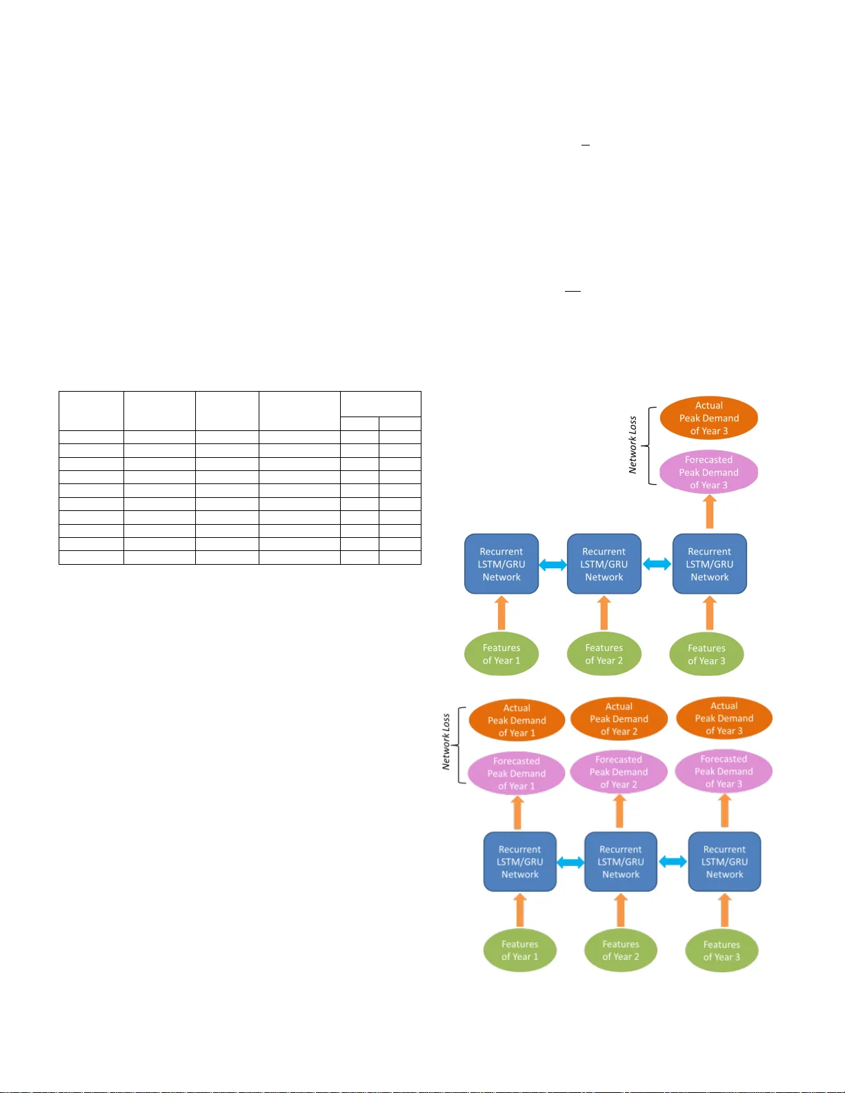
1949-3053 (c) 2019 IEEE. Personal use is permitted, but republication/redistribution requires IEEE permission. See http://www.ieee.org/publications_standards/publications/rights/index.html for more information. This article has been accepted for publication in a future issue of this journal, but has not been fully edited. Content may change prior to final publication. Citation information: DOI 10.1109/TSG.2019.2924183, IEEE Transactions on Smart Grid Abstract — Distribution feeder long-ter m load forecast (LTLF) is a critical task many ele ctric utility companies p erform on an annual basis. The goal of this task is to forecast the annual load of distribu tion feeders. The previous top-down an d bo ttom- up LTLF metho ds are unable to incorporate different levels of information. This paper proposes a hybrid m odeling method using sequence prediction for this classic and important task. The proposed method can seamlessly integrate top- down, bottom- up and sequential information hidden i n multi-year da t a. Tw o advanced sequence prediction models Long S hort-Term M emory (LSTM) and Ga ted Recurrent Unit (GRU) n etw orks a re investigated in this paper. They successfully solve the vanishi ng and explod ing gradient p roblems a standard recurrent neural network has . Th is p aper firstly explains th e theories o f LSTM and GRU networks and then discusses the steps of feature selection, feature engineering and model i mplementation in detail. In the end, a real-world a pplication example for a large urban grid in West Canada is provided. LSTM and GRU netw orks under different sequential c onfigurations a nd traditional models including bottom-up , ARIMA and feed-forward neural network are all i mplemented and compared in detail. T he proposed method demonstrates superior performance and great practicality. Index Terms — Long-term Load forecast, Sequence Prediction, Long Short-Term Memory network, Gated Recurrent Unit I. I NTRODUCTI ON ifferent fro m s hort-term load forecast (STLF), long-term load forecast (LTLF) problem refers to forecasting electrical po wer demand in more than one -year planning horizon for d ifferent p arts of a power s ystem [1 -3]. It is the essential foundation o f system p lanni ng activitie s in util ity companies. LTLF estab lishes a necessar y unders tanding of system adeq uacy for reliably supplying power to meet future customer demand. Peak demand is ofte n used as the forecast target b ecause it rep resents the worst case sce nario and needs to be tested against s ystem capac ity constraints. Long-term forecast of p eak demand at di stribution feeder level i s esp ecially important bec ause it is used as the input to assess the p ower deliver y cap acity during nor mal oper ation and the restoratio n cap ability during system contingencies for the ne xt few years. Onl y a fter proper forecast and assess ment, M. Dong is with Department of System Plannin g, ENMAX Power Corporation, Calg ary, A B, Canada, T2G 4S7 (e -mail: mingdong@ieee .org) L.S.G rumbach is with Auroki Analytics , Vanco uver, BC, Canada, V7L 1E6 (e -mail: ls grumbach@auroki.co m) utility co mpanies can reasonably plan lo ng -term i nfrastruct ure upgrades and m odifications [1-3]. Examples are transferri ng loads bet ween feeders, adding feeder tie-poi nts, building new feeders, installing new tr ansfor mers, building new substatio ns and etc. Therefore, distribution feeder LTLF signi ficantly affects the reliability of f uture grid , the satisfaction o f utilit y customers, the capital investment and f inancial outco me of utility companies. In general , LTLF m ethods can be grouped into the following three categories [4-6 ]: 1) Top-do wn Forecasting : this category foc uses on forecasting electricit y usage at a group-level suc h as t he load of all c usto mers or t he load of residential sector in a re gion [ 4 ]. Some methods use s ingle or combinations of un ivariate regression models such as AR IMA to analy ze the trend of loading change [ 7-9]. These m ethods only a nalyze the temporal load ing variable itself and are generally unacceptable for LTLF beca use lon g-term l oad change is str ongly d riven by external variables such as econo my, population a nd weather . To overcome this problem, so me methods use multivariate regression models such as feed-for ward neural network ( FNN) to analyze those external variables and their r elationships with the loadin g change [ 10 -14]. The advantage o f these methods is the statistical e xplicability. Ut ility companies ca n now forecast and explain future load change based on other variables forecasted by government or third -party agencies. These methods w ork w ell for regional or g roup-level load forecast but can be challenging when applied to s ystem co mpone nts such as individual distribution feeders. This is b ecause the top-do wn pr ocess o f allocatin g group -level load to individual members is subjective. T here is no clear way to reconcile the group-level i nformation with me mber-level in formation. It is also unrealistic to assume all me mbers s imply co mply with the group-level load behavior . In reality, a distrib ution feed er’s peak demand ca n be greatl y affected by its large loads and significantly deviates fro m its r egional load behavior. Therefore, in practic e top -down forecasti ng only pro vides an overall reference for manual chec k and adjustment of me mber -level forecast [4, 6 ]. 2) Bottom-up Forecasting: in contrast to top-down forecasting, this ca tegory r equires gathering bo ttom cus tomer load in formation to build a higher level f orecast. One approach of information gathering is conducting utilit y surveys or intervie ws. Long -term load infor mation such as A Hybrid Distribution Feeder Long-T erm Load Forecasting Method Based on Sequence Prediction Ming Dong, Senio r Member, IEEE and L.S.G rumbach D 97 1949-3053 (c) 2019 IEEE. Personal use is permitted, but republication/redistribution requires IEEE permission. See http://www.ieee.org/publications_standards/publications/rights/index.html for more information. This article has been accepted for publication in a future issue of this journal, but has not been fully edited. Content may change prior to final publication. Citation information: DOI 10.1109/TSG.2019.2924183, IEEE Transactions on Smart Grid expected sizes o f new loads, load matu ratio n p lan and/o r long-term p roduction plan is obtained, summarized a nd estimated as annu al loading ch ange. In practice, this is only done for large customers since those custo mers can substantially a ffect the feeder -level loading and it is too co stly to gather load plans from all custo mers [ 4 ]. Despite t he tremendous effort required to communicate with maj or residential developers, com mercial and industrial customers, inaccurate forecast ofte n occ urs with this app roach d ue to unreliable c ustomer infor mation and chan ge o f c ustomer plans over the forecasti ng horizo n. As an a lternative to surveys or interviews, some methods rely on the use of sub-load p rofiles [1 5-16]. Sub-load profiles are forecasted i ndividually or by clusters and then aggregated to a higher level. This is an effective approac h for SLTF. However, m issing statistical analysis of lo ad variation driven b y external factors ma de it unreliable for long -term forecast tas ks. 3) Hybrid Forecasting: this appro ach attempts to combine the advantages of top-do wn and bottom-up f orecasti ng. Unfortunately not m any research works were f ound in t his direction. One exa mple is the statisticall y-adj usted end -use model for household -level load forecast [1 7]. I t combines top-do wn weather, household and econo mic infor mation with bottom-up appliance information to forecast household -level load. No literature wa s found f or distribution feeder LTLF using similar methods. In respo nse to t he abo ve literature findings, the fir st contribution of t his paper is the estab lish ment of a h ybrid forecasting met hod that can effectively co mbine region al economic, de mographic a nd te mperature in formation with feeder-level lo ad infor mation in one mathematical model . As a result, this model can reflect the effects o f overall re gional drivers on feeder peak demand; it ca n also reflect lar ge customer load change, load composition, Distributed Energ y Resources (DER) and Electric Vehicle (EV) ado ption information specific to individual feeders. The second contribution of this pap er is the ado ption of sequence prediction model s to extract and utilize the long-term seq uential patterns of peak de mand to i mprove forecast acc uracy . Seq uence p redictio n is the pr oblem o f usi ng historical sequence infor mation to predict the next value or values i n a sequence [1 8]. Both LSTM and G RU networks a re commonly used advanced seque nce predictio n models . Compared to ARIMA, they suppo rt input a nd o utput with multiple features; co mpared to a standard recurrent ne ural network (RNN), the y solved the vanishing and exploding gradient prob lems and are therefore much more stable [1 9-24 ]. In a way, these models can co mbine t he adva ntages of univariate trending analysis and complex multivariate regression models . In recent years, researchers app lied the m to classic time-ser ies proble ms such as stock, weather forec asting and machine translatio n [25-27] . T hey ofte n outper for m traditional regression models such as FNN in these tas ks. I t was not u ntil very recently that some researcher s started to apply LST M and GRU to ST LF problem s in power systems [2 8- 30 ] . The application of LSTM and GRU to LTLF problems has not been fo und through literat ure r eview. T his paper aim s to fill this r esearch gap and explore the us e of LSTM and GRU networks under different sequenti al configurations for one o f the m ost classic and important long-term forec asting ta sks – forecasting individual feeder long-term peak de mand. The struct ure of the p roposed modeling method is shown in Fig.1. Raw t op -down features (related to economy, populat ion and temperature), ra w botto m-up features (related to customer load and DE R/EV adoption) , and previous -year peak de mand are all fed into a feature engineering module. For feature engineering, the concept of virtual feeder is p roposed to eliminate the data co rruption result ed fro m historical load transfer eve nts betwee n fee ders; feature nor malization is applied to normalize differen t types of feat ures to the same numerical scale; then principal co mponent analysis is applied to reduce the dimensionality of hig hly correlated features to improve model trai ning eff iciency and avoid over- fitting problems. After t he step of feature engineering, the dataset is constructed to a u nique multi-time step format u nder either many- to -many or many- to -one seq uential co nfigurations. The dataset is also split into train ing se t and test set for traini ng and eval uation purposes. Afte r model evaluation and net work parameter tunin g, a r eliable sequence p rediction model for distribution feeder LTLF is estab lished and can be used for future forecast. Fig.1. Wo rkflow of the propose d modeling method This paper firstly introduces the theo ries of LSTM and GRU network s. It then elab orates the workflow of feat ure selection, f eature engineering and model im pleme ntation as shown in Fig.1. In t he e nd, a real -world applicatio n to a lar ge urban grid in West Ca nada with 28 9 feeders is p resented and discussed in d etail. As p art o f the model evaluation, the proposed method is co mpared to traditional methods includin g bottom-up, ARIMA and FNN. It demonstrates superior performance over all of the m. II. I NTRODUCTI ON OF LSTM AND GRU M ODELS This section provides a brief introducti on to LSTM and GRU models and establish es the mathematical foundation f or the proposed metho d . Sin ce LSTM and GRU models are both based on RNN, this section firstly review s standard RNN and then explain s the working principles of LSTM and GRU and their advan tages ove r standar d RNN. 98 1949-3053 (c) 2019 IEEE. Personal use is permitted, but republication/redistribution requires IEEE permission. See http://www.ieee.org/publications_standards/publications/rights/index.html for more information. This article has been accepted for publication in a future issue of this journal, but has not been fully edited. Content may change prior to final publication. Citation information: DOI 10.1109/TSG.2019.2924183, IEEE Transactions on Smart Grid A. Recurrent Neural Network As shown in Fig.2, a RNN is a group of FNNs wh ere hidden neurons of the FNN at a previous time step are connecte d with the hidden neurons of the FNN at the follow ing ti me step. T he state of hid den neurons   is gen erated from    at the previous time step and the curr ent data input   by applying weights   and   . At each time step t , an o utput   is produced . This process co ntinu es for the next time step and so on. This way , RNN is able to make use of sequenti al inform ation and d oes n ot treat one time s tep as an isolat ed point. T his nature m ade RN N suitable for f orecasting task s where the output of current time step is not only based on the current input but als o the infor mation from previous tim e steps. Taking LTLF problem as an example, the current power demand is often not only related to the current year but also related t o the c onditions an d mom entum of the past few years . Fig.2 . Illustratio n of an unfolded RN N Althoug h RNN has a better performance than FNN when dealing with time-series d ata , the training of a RNN can be unstable due to an intrinsi c problem called vanishin g/expl oding gradient . T his problem is caused by the long distance during backpropag ation of ne twork loss from one FNN to another FNN a few time steps ago [1 9- 20 ]. Duri ng back propa ga tio n of RNN, g radient value may become very small a nd the training process loses tracti on; gradient value ca n also become very large and lead to overly large change of weig hts between updates. B. LSTM Model To solve the vanishing /explo ding gradient problem , LSTM model was proposed to improve the RNN structure [ 20 - 21 ]. Compared to standard RNN, LSTM introduces a specially designed LSTM unit to sophisticate dly control the flow o f hidden state inform ation from one time step to the next. The structure of LS TM unit is sh own in Fig.3 . Fig.3. A L STM unit diagram In Fig.3,    and  󰇍 󰇍   are the input vector and network hidden state vector at time st ep t .    is a vector stored in an external memor y ce ll. This memory cell carries infor mation between time steps, interacts with inp ut vecto r and hidden state vecto r and gets updated from one time step to the ne xt. Th is interactio n is completed through three control gates: forget gate, input gate a nd output gate. A forget gate ele ment   is calculated b y:      󰇍 󰇍 󰇍     󰇍 󰇍           (1) where  󰇍 󰇍       is the co ncatenated vecto r of previous hidden state vector  󰇍 󰇍    and the current input vector      is the sigmoid activatio n functio n ;  󰇍 󰇍 󰇍   and   are the weight vector and bias. The y are deter mined through net work training . Th e sigmoid ac tivation function outputs a value   between 0 and 1 . In the forget gate vector, each element   controls how the correspo nding ele ment in the ce ll state vector    gets kept or forgotten . 1 means keepi ng the element uncha nged and 0 means ze roing o ut the element . This is achieved by p ointwise mu ltiplying forget gate vector    by    and is mathematically give n later in (4). Following the infor mation flo w in Fig.3 , a temp orary cel l state element   is calculated by:      󰇛 󰇍 󰇍 󰇍     󰇍 󰇍          󰇜 (2 ) where  󰇍 󰇍       is the co ncatenated vecto r of previous hidden state vector  󰇍 󰇍    and the current input vector    ; tanh is the tanh activation function and outputs a value between -1 and 1 ;  󰇍 󰇍 󰇍   and   are the weight vector and bias. In p arallel with calc ulating   , the input gate   is calculated by:    󰇛 󰇍 󰇍 󰇍     󰇍 󰇍           󰇜 (3) where   and   are the weight vector and bias of   . Eventually the new cell state    at time step t is updated with previous cell s tate vect or     , forget gate vec tor    , input ga te vector     and tempo rary ce ll state vector  󰇍   by using pointwise multiplication and addition:                  󰇍   (4 ) This ne w cell state further deter min es the hidden state in the current neural network at time step t through the o utput gate    Si milar to   and   ,   is calculated b y:       󰇍 󰇍 󰇍     󰇍 󰇍           (5 ) Then, hidden state    at the current ti me step t is calculated by pointwise m ultiplying output gate vector    by the tanh function of    :  󰇍 󰇍        󰇛   󰇜 ( 6) Through (1) to (6 ), the current hidden state  󰇍 󰇍   is calculated with the use of    and  󰇍 󰇍    from t he p revious ti me step as well as the current input    .  󰇍 󰇍   is then used to p roduce network output   at the current time step . LSTM m odel inherits the ad vantages of R NN in d ealing with temporal forecast p roblems and also sol ve s the vanishing/exploding gradient problem by using t he LS TM unit . C. GRU Mod el GRU model is a ne wer sequence predictio n model invented in 20 14 by C ho et al . when they researched machi ne translation problems [2 2]. Co mpared to LSTM, GRU eliminates the use of the memory cell and uses only hidden state to car ry i nformation flow. It also merges the forget and 99 1949-3053 (c) 2019 IEEE. Personal use is permitted, but republication/redistribution requires IEEE permission. See http://www.ieee.org/publications_standards/publications/rights/index.html for more information. This article has been accepted for publication in a future issue of this journal, but has not been fully edited. Content may change prior to final publication. Citation information: DOI 10.1109/TSG.2019.2924183, IEEE Transactions on Smart Grid input gates i nto a single update gate. Generall y, GRU is more efficient than LSTM due to f ewer gates being used in the process . However, fro m t he accurac y p erspective , one model is n ot always better t han the other [ 23 ], except for certain language modeling tasks [24] . As a r esult , in practice LSTM and GRU m odels can be selected usi ng a trial and erro r approach for a spec ific problem or a specific dataset. This is also the appr oach suggested later in this pap er. The structure of a GRU unit is sho wn in Fig.4. Fig.4. A G RU unit diagram A reset gate element   is calculated b y:      󰇍 󰇍 󰇍     󰇍 󰇍           (7 ) where  󰇍 󰇍       is the co ncatenated vecto r of previous hidden state v ector  󰇍 󰇍    and the current input vector      󰇍 󰇍 󰇍   and   are the weight vector and bia s. An upd ate gate   element i s calculated by usi ng t he sa me input and activation function fro m (7) :      󰇍 󰇍 󰇍     󰇍 󰇍            (8) with different weight vector   and bias    Then follo wing the infor mation flo w illustrated in Fig.4, a temporary value   is calculate d by :      󰇛 󰇍 󰇍 󰇍    󰇟    󰇍 󰇍      󰇠 +   󰇜󰇛󰇜 Finally, the hidd en state ve ctor  󰇍 󰇍    at the current time step t is calculated with previous hidden state vector  󰇍 󰇍   , update gate vector  󰇍   and temporary vector  󰇍   by using pointwise multiplication and add ition :  󰇍 󰇍    󰇛    󰇍   󰇜  󰇍 󰇍      󰇍    󰇍   (1 0) Through (7)-(10), hidden st ate  󰇍 󰇍   is updated fro m one time step to the ne xt. It affects the neural net work o utput at e ach time step. Overall, LST M and GRU mod els have more co mplicated structures and m ore inter nal parameters th an standard RNN and FNN. As a resu lt they will need longer training time . However, they both solved the vanishing/explodin g gradient problem and are reliab le seque nce prediction models. III. F EATURE S ELECTI ON Feature selection i s normally th e first s tep of building a machine lear ning model [3 1]. By e mploying do main knowledge, useful ra w featur es related to the p roblem are analyzed and selected. In th e proposed hybrid m odel, both top-do wn features and bottom -up features related to distribution feeder peak demand are selected. T hey are elaborated as below. A. Top-down Features Top-do wn features descr ibe the overall d rivers in t he forecasted region. An nual economic, population a nd temperature features are considered in the model. T he historical and future ec ono mic and popul ation features can often be obtained fro m third -party co nsultants o r gover nment agencies [ 32]. T he historical te mperatures can b e ob tained from weather statistics data sources [3 3]. Future l ong -term temperatures, ho wever, are difficult to forecast. In practice, depending o n the conservativ eness o f system pl anning, the y can be nor malized to either the avera ge or extreme temperature p oint ob served in a region fro m the past fe w years. This is further explained i n Section V -E. 1) Econo mic Featu res: Different from short-ter m p ower demand, long-ter m po wer d emand is lar gely driven b y local economy. Annual r eal GDP gro wth (%) is the nominal G DP that excludes the effect of inflation rate; total employment growth (%) i s a nother i mportant econo mic feature. Higher employment means more p eop le hired in the co mmercial and industrial sector s and may p otentially use more electricit y; housing starts is the number o f residential units that are started to construct in a year in a region. This i ndicator is r elated to the increase o f reside ntial electricit y usage a nd can b e selected when available. Additional supplementar y econo mic features i nclude industrial pro duction indexe s and co mmodity prices [32] . They are more related to industrial loads and ca n be selected according to the industry co mposition in the forecasted r egion. 2) Po pulation Features: Population size significantly a ffects the residential load growth. Even when t he econo my s lows down, a stable population size can still support stable residential loading le vel. T his is because most o f the residential elec tricity d emand comes from e veryday household activities such as lighting, cooking, laundr y and so on. These activities are relatively immune to economic condition . Furthermore, population growth can result in the residential development which requir es electricity suppl y duri ng construction and a fter posses sion. In add ition, as part of the population, labor force in r eturn affects economic ac tivities and is related to the total employment gro wth. Therefor e, population growth (%) is sele cted in this work . Another useful population feature for some regions is net migration [ 31 ]. It is the a nn ual difference b etween the n umber o f i mmigrants and emigrants. This feature exclud es the p opulation ch ange d ue to natural birth a nd d eath and is more closely related to regional economic attrac tions. It can be considered for regions w ith frequent population migration. 3) Max/Min Temp erature: Dep ending o n forecasting s ummer peak d emand o r winter peak deman d, the highest te mperature during summer or the lo west te mperature during winter is selected for each year. T his is because summer peak de mand and win ter p eak demand often align with te mperature extremes due to cooling and heating electricit y u se [3 4 -35]. This correlation can be especially significant for summer because co oling almost al ways relies on electricity usa ge whereas h eating may rel y o n other energ y s ources such as 100 1949-3053 (c) 2019 IEEE. Personal use is permitted, but republication/redistribution requires IEEE permission. See http://www.ieee.org/publications_standards/publications/rights/index.html for more information. This article has been accepted for publication in a future issue of this journal, but has not been fully edited. Content may change prior to final publication. Citation information: DOI 10.1109/TSG.2019.2924183, IEEE Transactions on Smart Grid natural gas. Both the peak temperature value and the temperature change from the p revious year are selected . B. Bottom -up Features Bottom-up features d escribe the detailed feeder -level lo ad information. Large customer net load change, feeder load composition and DER/EV adoption growth are considered in the proposed models. 1) Large Customer Net Load Change : this feature is the estimated net load change of a ll large customers on the feeder . Examples of large custo mers can b e factories, shopping malls, office buildings and new r esidential developments. For a future year, t he load informa tion from eac h large customer c an be collected through utility survey or interview. So me may report gro wth while so me may rep ort red uction. The aggregated net cha nge is the summation of all these reported load changes fro m lar ge cus tomers on a feeder. Som etimes utility co mpanies may decide to further adjust the reported load changes based on their own understa nding i n c ase customers report unrealis tic information. 2) Feed er Loa d Composition (%): Distrib ution feeders have different t ypes of loads o n them and t hey respond to to p-do wn features in different ways. Fo r example, residential feeders are more r elated to tem perature and population while ind ustrial loads ar e more related to economy. Feed er load composition features can reflect this difference. Residential peak load percentage of a feeder is calculated by:                󰇛  󰇜 where   is the pea k lo ading of the feeder in t he summer or winter of previous y ear ;    is the lo ading o f residential load  at the feeder’s peaki ng time for   ;  is the total number of residential loads on thi s feeder. Similarly, co mmercial peak load p ercentage of a feeder is calculated by:                󰇛  󰇜 where    is the load ing of commercial lo ad  at the feeder’s peaking time for   ;  is the total num ber of commercial loads on thi s feeder. The industrial load perce ntage can be calculated in a similar way. It can also be calculated by:        ( 13 ) In actual app lication, only t wo features out of three need t o be selected because they are mathematically co rrelated with the third feature as ( 13 ) sho ws. 3) DER Ado ption Growth: Customer adoption of DER ma y reduce the peak demand of feeder s. T wo residential feeder s with si milar numbers of custo mers ma y have significa ntly different pea k de mand w hen they h ave very different DER adoption r ates. In regions where DER is a co ncern, featur es such as the forecasted numb er of new DER installatio ns or DER MW output can b e selected. DER ad option growth i tself can b e forecasted based o n cu stomer propensity anal ysis using methods such as [3 6 ] and is not discussed in this pap er. 4) EV Adop tion Growth: Customer adoption of EV ma y increase the peak de mand due to b attery char ging activities. In regions where EV is a concer n, features suc h as the forecasted number of newly purchased EVs can be selected . EV adop tion growth can b e forecasted based on customer p ropensit y analysis usi ng methods such as [3 7 ] and is not discu ssed in this paper. C. Previous-Year P eak Deman d Depending on forecasting summer pea k or winter peak, the previous year’s sum mer o r w inter peak demand is required in this model. The P revious- Year P eak Demand feature serve s as a b aseline wh ile all the discussed top-down and bottom-up features except feeder load co mposition (%) focus on the change of the following year. T ogether, all these features lead to the forecast of the following pea k demand. The f eatures d iscussed in this section are summarized in Table I. All the mandatory features ar e i mportant beca use these are the pr imary feat ures representing d ifferent factor s that a ffect feeder loading. They are also read ily available fr om a utility applicatio n p erspective. Optional features are specific to regions and may be i ncluded if applicab le. Mat hematicall y, whether to add an optional feature can also be determined by comparing the forecast acc uracy b efore and after adding it to the model. T ABLE I: F EATURES C ONSIDERED IN T HE P ROPOSED M ETHOD Feature Name Category Requireme nt Real GD P Growth (%) Top-dow n Mandatory Total Employ ment Grow th (%) Top-dow n Mandatory Population Gr owth (%) Top-dow n Mandatory Max/Min Tempe rature Top-dow n Mandatory Max/Min Tempe rature Change Top-dow n Mandatory Large Customer Net Load Chang e Bottom- up Mandatory Residential Pe ak Load Perce ntage Bottom- up Mandatory Commercial Pe ak Load Percentage Bottom- up Mandatory Previous-Ye ar Peak Demand Baseline Mandatory # of Housing S tarts Top-dow n Optional Industrial Pro duction Index Top-dow n Optional Commodity Price Top-dow n Optional Net Migration Top-dow n Optional DER Adoption G rowth Bottom- up Optional EV Adoption G rowth Bottom- up Optional IV. F EATURE E NGI NEERING Feature engineeri ng i s the st ep to trans form raw f eatures discussed in Sectio n III to proper features that ca n be fed into the pr oposed models for train ing [ 31]. The purpose of feature engineering i s to eli minate data noise, reduce model complexity and improve model accurac y. A. Virtual Feeder F eatures In pr actice, one si gnificant type of data noise that a ffects feeder p eak d emand over a long term co mes fro m the load transfer event s bet ween adj acent feeder s. A cer tain a mount o f customers can be s witched between ad jacent feeder s. This is often dri ven b y system o perational needs. For example, when feeder A’s load ing is get ting close to its ca pacity con straint, it is d ecided to transfer the c ustomers located o n a feeder br anch of feeder A to its adj acent feeder B so that both feeder A a nd B can continue to reliably sup ply their customers. In this case, load transfer crea tes a sudden load drop on feeder A and a sudd en load rise o n feeder B . This change d eviates from t he previous loadin g trend on both feeders and has nothing to do with any to p-do wn and bottom-up feat ures d iscussed in 101 1949-3053 (c) 2019 IEEE. Personal use is permitted, but republication/redistribution requires IEEE permission. See http://www.ieee.org/publications_standards/publications/rights/index.html for more information. This article has been accepted for publication in a future issue of this journal, but has not been fully edited. Content may change prior to final publication. Citation information: DOI 10.1109/TSG.2019.2924183, IEEE Transactions on Smart Grid Section III. Anot her example is mai ntenance driven load transfer. Feeder A may need to be d e-energized to maintain, replace or upgrade its substation breaker, conductors and cables. During this type o f maintenance work, feeder A needs to be sectionalized and c ustomers in each feeder section are transferred to multiple ad jacent feeders. Load transfer can be done through switching pre -installed branch switches and feeder-tie switches as il lustrated in Fig.5. Fig.5. An example of load transfer from feeder A to f eeder B Load tr ansfer is an almost i nevitable event in distribu tion grid. Over a long per iod of time such as a few years, a significant por tion of distribution feeders can be affected by this ev ent. Load transfer events create data noise a nd significantly reduce the ac curacy of the mod el if ra w features are directly used for modeling. To overcome t his pro blem, t his pap er proposes a concept called virtual feeders. This unique technique will ensure the continuity of feeder loading trend in the dataset. Fo r one area, a virtual feeder can be created and it is the average o f the adjacent feeders which had load transfer e vents in the model training perio d. Instead of using features of individual feeders in this area a s training records, the feature s of virtual feeder are generated and used. T he Previous- Year Peak Demand feature of the virtual feeder can be estimated b y:                󰇛  󰇜 where   is the Previous-Yea r Peak Demand feature of adjacent feeder i involved in historical load transfers during the model training p eriod ;   is the Previous- Year Peak Demand feature of the virt ual feeder; p is the number of adjacent feeders that have switching eve nts during the model training p eriod. p is normally 2 but can be greater than 2 for multi-feeder switchin g during feeder maintenance activities. Similarly, large customer net load change feature LC of virtual feeder can be calculate d by:             󰇛  󰇜 DER and EV adoptio n growth on the virtual feeder can be calculated by:             󰇛  󰇜             󰇛  󰇜 where   and   are the DER and EV growth features of feeder i. Residential Peak Load P ercentage and Commercial P eak Load P ercentage R and C of the virtual feeder can be estimated b y:                 󰇛  󰇜                 󰇛  󰇜 where   and   are the residential and co mmercial pea k load perce ntage features of feeder i. The to p-do wn fea tures in T able I do not need to be updated for virtual feeders as the y represent t he governing regio nal characteristics. B y creating virtual feeder f eatures, the data noise co ming fro m lo ad transfer eve nts ca n b e ef fectively eliminated. B. Feature Norma lization This is a necessary step because t he features disc ussed in Section III use different units and have large magnitu de differences a mong t hem. There are many ways of nor malizing raw features [ 31], f or exa mple, the Min -Ma x nor malization can normalize features to the value range o f [0,1] . It is given by:             󰇛  󰇜 where for a spec ific feature, MAX is the maximum o bserved value in this feature  MIN is the minimum observed value in this feature  C. Principal Compo nent Analysis Table I contains many econo mic and population feat ures. These features emphasize d ifferent aspects bu t are highly correlated. For exa mple, Net Migration can i ncent Real GDP Growth and lead to Housi ng Star ts Gro wth; To tal Employment Gro wth often goes hand- in -hand w ith Real GDP Growth. These feat ures are not independent and can be aggregated using principal c o mponent analysis (PCA) [31]. This is i mportant because LT LF has to rel y on a nn ual data points. No t like ST LF which often uses hourly data p oints, annual data points are lim ited in number. Reducing fea ture dimensionality can improve model accuracy a nd avoid over-fitting prob lems. PCA is defined as an orthogonal linear tra nsformation that maps the data w ith multiple variables to a new co ordinate syst em . In th is n ew coor dinate s ystem, coordinates a re orthogon al (independen t) to each other and the greatest d ata variance direction aligns with the first coordinate ( i.e. the first principal component), the second greatest variance d irection aligns with the second coordinate, and so on . Mathematically , the transformation is defi ned as: 󰇥              󰇛  󰇜 where X is the normalized mean-shifted data matrix with k feature columns (each column is subtracted by the column mean) ;  is a k - by - k matrix whose co lumns are eigenvectors of    ; D is the dia gonal matrix with ei genvalues   on the 102 1949-3053 (c) 2019 IEEE. Personal use is permitted, but republication/redistribution requires IEEE permission. See http://www.ieee.org/publications_standards/publications/rights/index.html for more information. This article has been accepted for publication in a future issue of this journal, but has not been fully edited. Content may change prior to final publication. Citation information: DOI 10.1109/TSG.2019.2924183, IEEE Transactions on Smart Grid diagonal and zeros ever ywhere else;  is the ne w data matrix in which each colu mn is an in dependent feature pro jected to a principal co mponent. After the transfor mation, t independent features can be selected from T based on the Prop ortion o f Variance Explained (PVE). PVE of t features indicate s t he amount of information (variance) attributed to these features and is mathematically given as b elow:                   󰇛  󰇜 An exa mple of transfor ming four econo mic -population features to two independe nt features EP1 and EP2 along two orthogonal principal co mponents is shown in Table II. T wo fe atures are selected because their co rresponding PVE value using ( 22 ) is 9 7.1%. T his means most of the i nformation fro m the original four features can be kept in the t wo newl y constructed feat ures EP1 and EP2 . T ABLE II: A N E XAMPLE OF P RINCIPAL COMPONENT ANALYSIS Real GD P Growth (%) Total Employ ment Growth (%) Population Growth (%) Net Migration ( ’ 000 Persons) New Fe atures After PCA EP1 EP2 14.2 4.9 2.9 17.6 -0.64 0.44 9.1 2.7 2.2 12.4 -0.16 0.31 -2.5 -0.5 2.2 12.9 0.33 -0.31 2.2 1.3 2.6 18 .0 -0.06 -0.17 3.2 2.0 1.0 4.0 0.38 0.32 3.5 3.4 2.7 14.3 -0.19 0.02 2. 3 2.6 2.6 19.1 -0.17 -0.12 3.9 3.2 3.4 22 -0.44 -0.18 -0.2 1.3 3 .0 24.9 -0.19 -0.42 - 3. 2 -2.6 0.3 -6.5 1.14 0.11 V. M ODEL I MPLEMENTATI ON After feature selectio n and feature engineering, this section elaborates step s of model implementation. T wo d ifferent sequential co nfigurations, t he construction of multi-time step dataset, the split of training and test set, the setup and tuning of network parameters and the forecasting process are explained as follo ws. A. Sequential Con figuration As a RNN neural network, LSTM and GRU each have three different sequential co nfigurations: one- to -many, many- to -many and m an y- to -one [21, 2 5-26]. Many- to -man y and many- to -one co nfigurations are b oth suitable for sequence prediction problems. Their sche matics are sho wn in Fig.6 . The proposed method ai ms to use three consecutive y ears’ features to forecast the third year’s future peak demand. Many- to -one configuration precisely captures this 3- to - 1 relationship; in comparison, many- to - many configuration also includes two previous years’ actua l and forecasted peak demands . D uring the forecas t process, since the actua l p eak demands of year 1 and year 2 are alread y known , producing forecast ed value s of year 1 and year 2 is not meaningful. However, the inclusion o f the values of the se two years do es make a difference on the network lo ss function calculati on during the network trai ning process . In order to match with the Mean Absolute Percentage Error (MAPE) later used for model evaluation in Sectio n VI , Mean Absolute Err or (MAE) is selected to construct the net work loss functions. The lo ss function for many - to -one configuration is:                 󰇛  󰇜 where n is the training batch size;   is the third year’s actual peak demand of   record in the traini ng batch;   is the third year’s forecasted peak de mand of   record in the training batch. The loss function for many- to - many configuration is:                        󰇛  󰇜 where n is the tr aining batch size;    is the   year’s act ual peak d emand of   record in the training batc h;    is the   year’s forec asted p eak demand o f   record in t he training batch. (a) Many- to -O ne sequential configuratio n (b) Many- to -Many sequential configur ation Fig. 6. Ma ny- to -O ne and Many- to -Ma ny sequential conf iguration 103 1949-3053 (c) 2019 IEEE. Personal use is permitted, but republication/redistribution requires IEEE permission. See http://www.ieee.org/publications_standards/publications/rights/index.html for more information. This article has been accepted for publication in a future issue of this journal, but has not been fully edited. Content may change prior to final publication. Citation information: DOI 10.1109/TSG.2019.2924183, IEEE Transactions on Smart Grid During the training process, each training batch ’s network loss is calculated and back p ropagated to update the weights between neurons. T heoretically, the ad vantage of man y- to -one configuration i s t hat it s los s function   is specif ic to the desired forecast target and the training should there fore make its best effort to minimize the error between the t hird year’s actual and forec ast ed peak demand. However, when the act ual peak demand fluctuates significantly within the t hree-y ear period , emphasizing only the third y ear’s res ult may lead to a biased model . In comparison , many- to - many co nfiguration’s loss function   measures the average of all three years’ errors. W hen the output fluctu ation is lar ge, this config uration will b e able to filter uncertaint ies and produce more consiste nt output year over year . The effect of these configurations will be further tested and discussed in Section VI. B. Multi-time Step Da taset Different fro m traditio nal datasets u sed for FNN or other supervised learning models, LSTM and GRU models require data rec ords to be grouped by a fixed number of time ste ps. This type of grouping i s done for all feeders and all avai lable years. T wo dataset example s structured to m any- to -one a nd many- to -many configuratio ns are shown in Tab le I II and Table IV. Taking d ata record ID 1 in T able I II and Table IV as an example , 2009 /2 010/2011 are three forecast years a nd 2 011 is the fin al forecast year (Year- 3) w hose peak de mand is t he forecast tar get. The recor d has three ro ws a nd each row has features fro m a previous year and a forecast year. The previous year features are from 2 008/20 09/2010 ; the forecast year feature s ar e fro m 20 09/2010/2 011. It should be noted that the forecast year features in 2011 are forec asted values because in real app lication year-3 is a future year and its act ual features are unknown. Compar ing T able III and Table IV, the difference bet ween many - to -one and many- to - many datasets is the i nclusion of actual peak de mand in 200 9 and 2 010 in th is data r ecord. T his difference aligns with the network loss function difference explained in Section V - A. C. Training/Test Set Sp lit The multi-ti me step dataset should be r andomly split into a model trai ning set and test set by recor d. The training set is used to trai n the model; the test set is used to evaluate the model accuracy. A typical split ratio is 8 0% for training and 20% for testing. Model evaluation details will b e disc ussed in Section VI. D. Network Paramete r Setup and Tuning Like a t ypical F NN , a LSTM/GRU net work conta ins a specific number o f hidden layers, a speci fic number of neurons in each hidden layer and a sp ecific t ype o f acti vation function for neuron s. There is no direct way to deter mine these parameters rather than tr ying different co mbinations until acceptable results ar e obtained through model evaluation. Optimization methods such as grid searc h and ra ndom search ca n be co nsidered to facilitate the pr ocess [31]. Grid search initializes a finite set of reasonable values as the search space. For example, the numb er of hidden layers  {1,2,3} and the number of neurons  {10,15,2 0} can yield in to tal 9 combinations. Gr id search goes through all these 9 combinations a nd choo ses t he co mbination with the best performance. Random search enumerates parameter combinations r andomly inste ad o f exhaustively traversing all of them. Other tu ning algorith m such as B ayesian optimizati on is not recommended due to the li mited size of our network. E. Forecasting Proce ss Once the m odel is established after training and evaluation , it can be used to forecast po wer demand in future years . Next year’s forecasted econo mic and po pulation features ca n b e obtained from government or third-party agencies and are usually produced b y their eco nomists. It should be noted t he se forecast results could also contain er rors. However, like in a ny multivariate LTLF methods, these numbers are often accur ate enough, especially for the foreca st of immediate co ming yea rs. However, o ne feature that can hardly be forecasted accurately is the Max/Min T emperature of future years. To avoid this pro blem, p lanning en gineers usually nor malize future te mperatures to a conservative value and prod uce future forecast using this co mmon basis. For exa mple, if the maximum temperature in th e past decade is 35  . W hen forecasting t he next few years ’ lo ading, a safety mar gin 1  can be added to the histo rical hi gh a nd 36  can be consistently used for forecast moving for ward. Another benefit of the establi shed forecasting model is that it can be used to retroactively normalize historical feeder peak demands using a statis tical temperature so that historical yearly load ings can now be compared on the same basis. As a result, a more objective trend can be o btained. Rare eve nts suc h as World Cup ga mes ma y lead to abnormal load ing that can not b e effectively forec asted based on historical data. Extra safet y margins ca n be ad ded to the forecasted values i n these cases . The forecast can b e per formed co ntinuously one year after another. For example, if 2019 is the first year to forecast , 201 9 ’s feeder p eak demand will be firstly forecasted and then it is combined with 20 18 and 201 7 to forecast 20 20 ’s peak demand. T his proce ss co ntinues until all years i n a di stribution planning horizon (e.g. next three y ears) are forecasted . I t should be noted the accuracy level may gradually decr ease but it is usually minor for the imm ediate next few years. VI. A PPLICATIO N E XAMPLE The proposed approach was applied to a large urban grid in West Cana da to establish both summer and winter long-term peak dem and forecasting m odels for its distri bution feed ers that serve va rious types of loa ds . A. Description of Da taset In total 289 distr ibution feeders were sele cted and their past 14 -yea r a n nua l d at a (2 0 04 -2 01 7 ) wer e use d t o cr ea te the dataset. During this period, 182 of them had two-feede r or mu l t i - f e e d e r l o a d t r a n s f e r e ve nt s a mo n g t h e m a n d w e r e converted to 87 virtu al feeders. The remainin g 107 fee ders are actual feeders that either have no transfer events o r have very short transfer periods that do not affect the correct gathering of annual peak demand. In total 1,997 valid three-y ear records were produce d in the data format descri bed in Table I II and Tab le I V fo r bo th su mmer a nd winter . In o rder to r evea l 104 1949-3053 (c) 2019 IEEE. Personal use is permitted, but republication/redistribution requires IEEE permission. See http://www.ieee.org/publications_standards/publications/rights/index.html for more information. This article has been accepted for publication in a future issue of this journal, but has not been fully edited. Content may change prior to final publication. Citation information: DOI 10.1109/TSG.2019.2924183, IEEE Transactions on Smart Grid T ABLE III: D ATASET E XAMP LE FOR S UMMER P EAK D EMAND F ORECAST (M ANY - TO - ONE C ONFIGURAT ION ) Data Record ID Feeder ID Forecast Year Previous Ye ar Features Forecast Year F eatures Year-3 Peak Demand (Year 3) Previous- Year Peak Demand Residential Peak L oad percentage Commercial Peak L oad percentage EP1 EP2 Maximum Temper ature Maximum Temper ature Change Large Customer Ne t Load Change 1 1001 20 09 433 A 66.5% 10.2% -0.64 0.44 33.3  0.7  42 A 550 A (2011) 1001 20 10 502 A 63.1% 11.1% -0.16 0.31 32.0  -1.3  34 A 1001 2011 554 A 63.0% 11.3% 0.33 -0.31 35.4  3.4  0 A 2 1001 20 10 502 A 63.1% 11.1% -0.16 0.31 32.0  -1.3  34 A 521 A (2012) 1001 2011 554 A 63.0% 11.3% 0.33 -0.31 35.4  3.4  0 A 1001 2012 540 A 59.4% 12.7% -0.06 -0.17 33.2  -2.2  -21 A … … … … … … … … … … 238 1 32 1 20 10 317 A 94.2% 5.8% -0.16 0.31 32.0  -1.3  0 A 3 31 A (2012) 1 32 1 2011 323 A 93.8% 6. 2% 0.33 -0.31 35.4  3.4  10 A 1 32 1 2012 329 A 94.1% 5. 9% -0.06 -0.17 33.2  -2.2  0 A … … … … … … … … … … T ABLE IV: D A TASET E XAMPLE FOR S UMMER P EAK D EMAND F ORECAST ( MANY - TO - M ANY CONFIGURATION ) Data Record ID Feeder ID Forecast Year Previous Ye ar Features Forecast Year F eatures Forecast Year Peak Demand Previous- Year Peak Demand Residential Peak L oad percentage Commercial Peak L oad percentage EP1 EP2 Maximum Temper ature Maximum Temper ature Change Large Customer Net Load Change 1 1001 20 09 433 A 66.5% 10.2% -0.64 0.44 33.3  0.7  42 A 502 A 1001 20 10 502 A 63.1% 11.1% -0.16 0.31 32.0  -1.3  34 A 554 A 1001 2011 554 A 63.0% 11.3% 0.33 -0.31 35.4  3.4  0 A 550 A 2 1001 20 10 502 A 63.1% 11.1% -0.16 0.31 32.0  -1.3  34 A 5 54 A 1001 2011 554 A 63.0% 11.3% 0.33 -0.31 35.4  3.4  0 A 550 A 1001 2012 550 A 59.4% 12.7% -0.06 -0.17 33.2  -2.2  -21 A 521 A … … … … … … … … … … 238 1 32 1 20 10 317 A 94.2% 5.8% -0.16 0.31 32.0  -1.3  0 A 323 A 1 32 1 2011 323 A 93.8% 6. 2% 0.33 -0.31 35.4  3.4  10 A 329 A 1 32 1 2012 329 A 94.1% 5. 9% -0.06 -0.17 33.2  -2.2  0 A 331 A … … … … … … … … … … Fig .7 . MAPE distr ibution in summer T ABLE V: S UMMER R ESULTS LSTM(Many - to -One) GRU (Many- to -One) LSTM(Many - to -Many) GRU(Many- to -Many) MAPE(%) 6.67 6.92 6.54 6.79 Cumulative Pe rcentage w ith MAPE  10% (%) 85.12 82.70 84.43 82.01 Model Training T ime (s, Epoch=2 00) 202.46 164.09 200.33 162.28 105 1949-3053 (c) 2019 IEEE. Personal use is permitted, but republication/redistribution requires IEEE permission. See http://www.ieee.org/publications_standards/publications/rights/index.html for more information. This article has been accepted for publication in a future issue of this journal, but has not been fully edited. Content may change prior to final publication. Citation information: DOI 10.1109/TSG.2019.2924183, IEEE Transactions on Smart Grid Fig. 8. MA PE distribution in win ter T ABLE VI: W INTER R ESULTS LSTM(Many - to -One) GRU (Many- to -One) LSTM(Many - to -Many) GRU(Many- to -Many) MAPE(%) 5.09 5.20 6.15 6.08 Cumulative Pe rcentage with MA PE  10% (%) 87.28 86.03 83.04 83.04 Model Training T ime (s, Epoch=2 00) 200.11 161.20 203.85 163.59 models ’ tru e forecastin g capability , for eve ry third y ear, inste ad of using the actual values , forecas ted economic and populat ion features prior to that year were used. The 1,997 records were split into 1,597 records for train ing and 400 records for testing based on the 80%/20% split rat io. To evalu ate th e m odel’s forecast accuracy , the trained model was tested on the 400 test records and compar ed to the actual peak deman d values. B. Results of LSTM and GRU under Two Sequential Configurations LS T M a nd GR U mo d el s w e r e i mp l e me n t e d wit h b o th many- to -ma ny and man y- to -one config uratio ns for su mmer and win ter separately. Each configu ration uses 8 input features as listed in Table III and IV. Summer results are summ arized in Fig.7 and Table V; winter resu lts are summ arized in Fig.8 and Table VI . For each model, two hidden layers were composed. One hidden layer is a LSTM/GRU layer which contains hidden states and the other hidden lay er is a regular neural network layer connec ting to the output layer. Each h idden lay er contai ns 6 neurons. The rectifie d linear unit (ReLU) activation function is used in ea ch neuron. MAPE was chosen as the fir st accuracy metric. It is co mmonly used for measurin g prediction error and is given as:                     󰇛  󰇜 where m is the total number of test records;   is the forecast ed value of   record ;   is the actual value of   record. Based on the MA PE results, histograms are produced to present the error distri butions in Fig.7 and Fig.8. The records with less than or equal to 10% MAPEs are counted and its percentage num ber against the total number of records (i.e. 400) is calculated. This percentag e number directly reflects how m a n y f o r e c a s t e d r e c o r d s h a v e h i g h c o n f i d e n c e l e v e l s . Another aspect of th e evaluat ion is in regards to the m odel training tim e. Once a model is trained, the time required for testing using the trained model is almost negligible and is therefore not include d for comparis on. The hardw are computati onal environm ent for this application example is Inte l i7-6700K CPU @ 4.00GHz with 4 Cores and 16GB DDR4 RAM memory. The softw are environm ent is Windows 10 and Python 3.5 with Tensorflow backend. The total number of training epochs w as set to 200 with a batch size of 10. A few observations ca n be drawn from the obtained r esults:  Overall, all models and configuratio ns are quite acc urate. This shows the great value of the proposed method. It was found that most large errors are attributed to abnor mal load behaviors during two dra matic economic downtur ns in 2009 and 2015 -2016 in the interested region. Pr ior to these downturns, no one forecast ed the eco nomy a nd po pulation features corr ectly and the inp ut errors lead to the po wer demand forecast erro rs in the results.  LSTM and GRU have very close accuracy le vels. Fro m MAPE and Cumulative Perce ntage metrics, LST M slightly outperformed GRU in sum mer in both con figurations while GR U slightly o utperformed LSTM in winter under the many- to -many configurati on. T he difference s bet ween them are ver y small.  In winter, many- to -one configurations noticeably outperformed many- to -man y configuration s with both 106 1949-3053 (c) 2019 IEEE. Personal use is permitted, but republication/redistribution requires IEEE permission. See http://www.ieee.org/publications_standards/publications/rights/index.html for more information. This article has been accepted for publication in a future issue of this journal, but has not been fully edited. Content may change prior to final publication. Citation information: DOI 10.1109/TSG.2019.2924183, IEEE Transactions on Smart Grid LSTM and GRU m odels. However, in s ummer the accuracy difference beco mes marginal a nd many- to -many configuration beco mes slightly better than many- to -one configuration in M APE (%) . One expla nation for t his interesting ob servation is t hat the summer loading reco rds in the histor ical timespan have larger fluct uations due to the rapidl y increasing use of air co nditioners year over year in the region . O n the contrary , nat ural gas is the mai n source of heatin g in winter in the re gion a nd does not consume much electricity . T herefore, if economic and population changes are excluded , the load i ng of winter months between adj acent years is relatively stable. In Section V, it has b een discussed that many- to -one configuration onl y focuses o n the desired output and ca n be more accurate i f the yearl y fluctuation is lo w. This is t he reason many- to -one configuration is no tic eabl y more accurate in winter. In compariso n, m any- to -man y configurations are more immune to output fluctuation because its network loss fu nction automaticall y smooth out the differences within three co nsecutive years a nd therefore produces a more neutral forecast model thro ugh training. This is t he r eason the advantage of man y- to - many configuration is reveal ed in s ummer while t he advantage of many- to -one con figuration is under mined.  Fro m the training ti me perspective, GRU is significa ntly faster than LST M. This was expected because of fewer gates used in the model . The ti me difference bet ween many- to -many and many- to -o ne configurations is negligible. T his is becau se the computation ti me required for calculating different lo ss functions is not mu ch different in the given computation al environment. Since LTLF is not p erformed in real -time and all the listed training t imes are ge nerally acceptab le, it is r ecommended that all 8 models are tested and the best models get selected for future sum mer and winter forecast separ ately. C. Improvement By Using Virtual F eeders The m ost ac curate model and configuration by MAPE (%) from Tab le V and VI were selected and tested without the use of virtual feeders. T heir MAPE results are sho wn in Table V II . T ABLE V II : I MPROVEMENT BY USING V IRTUAL F EEDERS Use Virtual Feeder Features? Summer: L STM Many- to -Many MAPE (%) Winter: L STM Many- to -O ne MAPE (%) No 14. 27 % 11. 48 % Yes 6.54% 5. 09 % Significant perfor mance i mprovement can be o bserved after using the proposed v irtual fee der f eatures to eliminate data noise caused b y the load transfer events. D. Comparison to Other Mod els As p art of the model evalua tion, the p roposed model was compared to various trad itional models estab lished as below. Virtual feeder features ar e als o used in these models.  Bottom- up mod el: As disc ussed in Sectio n I, only Lar ge Customer Net Load Change feature was gathered and added to the Previous- Year Peak Demand to calculate the following year’s peak de mand.  ARIMA model : T he sa me 14-year loadin g data of 28 9 feeders were used. For each feeder, its first 13 -year pea k demand values were fed into a ARIMA (2,0,0) model for trai ning . ARIM A ( 2,0,0) was found to give the b est forecast result among dif ferent ARIM A order parameters for this dataset. T hen the peak de mand values i n 2017 were forecasted and co mpared to th e true v alue s to calcualte MAPE.  One-year FNN : The same 14 -year data o f 289 feeders were used. For each feeder, o nly one year features are used to forecast. Each train ing record is li ke ea ch ro w i n T able I V. A trad itional FNN model is used. T he input layer has 8 neurons (features) and two hidd en la yers each have 6 neurons. Re LU activation functions ar e used in the hidd en and output layers.  Three -year FNN : The same 14 -year data of 289 feeders were used. Instead o f using the LSTM /GRU neural network, a traditional FNN m odel is used to incorp orate all the features o f three consecutive years (i n total 24 features) to forecast the t hird year’s p eak de mand. T he input layer has 24 neurons and two hidden layers each have 12 neurons. ReLU ac tivation functions are used in t he hidden and output layers. T ABLE V III : P ERFORMANCE C OMPAR ISON OF DIFFERENT MODELS Model Summer MAP E (%) Winter MAP E (%) Best LST M/GRU Models 6.54 % 5. 09 % Bottom- up 16.61% 14.80% ARI MA 14.51% 11.33% One-year FNN 14. 62 % 10 . 19 % Three-year F NN 8.51 % 7.88% As shown in T able V III , the proposed model outperformed all other models for both summer and winter forecastin g. VII. C ONCLUSION S This paper presents a novel and co mprehensive method for distribution feeder long- term load forecast. Compared to previous methods, t h e advantages of t his method are:  It uses a hybrid model which can seamlessly in tegrate different levels o f information including both top -down and bottom-up features. It can therefore capture the relationship s among feeder pea k demand , o verall regional drivers and individual feeder load details .  It uses ad vanced sequence p rediction models LSTM and GRU to effectively capture and leverage the sequentia l characteristics of m ulti -year data to improve forecast accuracy. The p roposed method was ap plied to a lar ge urb an grid in West Canada. LST M and GRU models under two sequenti al configurations and a few dif ferent trad itional models were all implemented a nd compared in detail. T he p roposed method with the use of virtual feeder demonstrated superi or performance for both summer and winter forecasts compar ed to traditional models. Overall , LSTM and GRU models have similar per formances. GRU model is faster than LSTM model. The performances of many- to -many and many- to -o ne sequential co nfigurations are affected b y the o utput fluctuation level between adj acent years. Since the training ti mes are not very long, it is reco mmended to evaluate b oth LSTM and GRU models under two sequential co nfigurations and cho ose the best performers for forecast ap plication. 107 1949-3053 (c) 2019 IEEE. Personal use is permitted, but republication/redistribution requires IEEE permission. See http://www.ieee.org/publications_standards/publications/rights/index.html for more information. This article has been accepted for publication in a future issue of this journal, but has not been fully edited. Content may change prior to final publication. Citation information: DOI 10.1109/TSG.2019.2924183, IEEE Transactions on Smart Grid R EFERENCES [1] H. L. Willis, Power Distribution Pl an ing Refere nce Book , CRC p ress, 1997. [2] H. Seifi and M. S. Sepasian, Electric Power System Planning: Issues , Algorithms and Solutions , Springer Science & Business Media, 2011. [3] F. Elkarmi, ed. , Power System Planning Technologies and Applications: Concepts, Soluti ons and Managem ent , IGI Global, 2012. [4] W. Simpson and D. G otham. “Standard approac hes to load forecasting and rev iew of Manitoba Hy dro load forecast for n eeds for and alternatives To (NFAT), ” The Manitoba Public Utilities Board, Canada. [Online].Available : http://www .pub.gov.mb.ca/nfat/p df/load_forecast_sim pson_gotham.pdf [5] Midwest I SO, “Peak forecasting methodol ogy review , ” Mid west I SO, Carmel, I N, USA. [Online].Available : https://leg alectric.org/f/2011/10/pe ak -for ecasting-methodology -review- whitepaper-2011.p df [6] BC Hydro (De c. 2012), “Electric load for ecast: Fiscal 2013 to F iscal 2033, ” BC Hy dro, Canada. [Online]. Available: https://www .bchydro.com/content/ dam/BCHy dro/custom er -portal/docu ments/corporate/re gulatory- pl FNNing-documents/integ rated-resource- pl ans/current-plan/2 012-electric-load-fo recast-report.pdf [7] T. Al -Saba and I . El - Amin, “Artificial n eural networ ks as a pplied to long-term demand f orecasting, ” Artificial Intelligence in Engineering , vol. 13, no. 2, pp. 189 -197, 1 999. [8] M. Askari and A. Fetanat, “Long -term load forecasting in powe r s ystem: Grey sy stem prediction-based models, ” Journal of Ap plied Sciences , vol. 11, no. 16, pp. 303 4-3038, 2011. [9] F. Kong and G. Song, “M iddle-long power load forecasting based on dynamic grey prediction and suppo rt vector machine, ” Int. J. Adv. Comput. Tech nol , vol. 4, no. 5, pp. 148 -156, 201 2. [10] A. A. El Deso uky an d M. M. Elkateb, “ Hybrid adaptive techniques for electric-load forecast using A NN and ARI MA, ” IEE Proceed ings - Generation, Transmiss ion and Distribut ion , vol. 147, no. 4, pp. 213-217, July 2000. [11] R. J. Hyndman and S. F an, “ Density forecasting for lo ng-term p eak electricity demand, ” IEEE Transactions o n Power Systems , vol. 25, no. 2, pp. 1142-1153, May 2010. [12] M. S. Kandil, S. M. El-Debeiky and N. E. Hasanien, “ Long-term load forecasting for fast developing utility using a knowledge-based expert system, ” IEEE Transactions on Power Systems , vol. 17, no. 2, pp. 491-496, May 2002. [13] T. Hong, J. Wilson and J. Xie, “ L ong term p robabilistic load Forecasting and normalization with hourly information, ” IEEE Transactions on Smart Grid , vol . 5, no. 1, pp. 456-462 , Jan. 2014. [14] Y. Go ude, R. Nedellec and N. K ong, “ L ocal sh ort an d middle term electricity load forecasting with semi-parame tric additive models, ” IEEE Transactions on Sm art Grid , vol. 5, n o. 1, pp. 440-446, Jan. 2014. [15] B. Stephen, X. Tang, P . R. H arvey, S. G alloway and K. I. Jennett, “ Incorpo rating practice t heory in s ub - profile models for short term aggregate d residential load forecasting, ” IEEE Transactions on Smart Grid , vol. 8, no. 4, pp. 1591-1598, Jul y 2017. [16] Y. Wang, Q. Chen, M. Sun, C. Kang and Q. Xia, “ An ensemble forecasting method fo r the aggregate d load With subprofile s, ” IEEE Transactions on Sm art Grid , vol. 9, n o. 4, pp. 3906-3908, July 2018. [17] K. Train, J. Herriges and R. Windle , “Statistic ally adjusted engineering models of end-use load curves, ” Energy , vol. 10(10), pp. 1103-1111, 1985. [18] R. Sun and C. L. Giles, "Sequence learning: from recognition and prediction to sequential decision making," IEEE Intellige nt Sy stems , vol. 16, no. 4, pp. 6 7-70, July-Aug. 2001. [19] J. F. Kol en and S. C. K reme r, “ Gradient flow in recurrent n ets: the difficulty of learning long- term dependencies, ” A Field Guide to Dynamical Rec urrent Networks , I EEE, 2001 [20] S. Hochreiter and J. Schmidh uber, “ Long sh ort-term memory , ” Neural computation , vol.9, pp.1735-1780, 1 997. [21] Sutskever, Ilya, Oriol Vinyals, and Quoc V. Le. “ Sequence t o sequence learning with neural networks, ” Advances in Neural Information Processing Systems , pp. 3104-3112, 2014. [22] K. Cho, B. Van Merrië nboer, C. Gulcehre , D. Bahdanau, F. Bougares, H. Schwenk and Y. Bengio, “Learning p hrase representations using RNN encoder-decode r for statistical machine translation, ” arXiv preprint , arXiv:1406.1078, 2014. [23] J. Chung, C. Gulcehre, K. Ch o and Y. Bengio, “Empirical evaluation of gated recurrent neural networks on sequ ence modeling, ” arXiv preprint arXiv:1412.35 55, 2014. [24] R. Jozefow icz, W.Zaremba, and I .Sutskever, "An empirical exploration of recurrent network architectures." In International Conference on Machine L earning, pp. 2342-2350, 2015. [25] H. Y. Kim and C. H. Won, “Fore casting the volatility of stock price index: A h ybrid model integrating LSTM with multiple GARCH-type models”, Expert Systems with Appli cations , vol. 103, pp. 25 -37, Aug. 2018. [26] X. Qing and Y. Niu, “Hourly day -ahead solar irradiance pre diction using weather for ecasts by L STM”, Energy , vol . 148, pp. 461-468, Apr.20 18 [27] S. P. Singh, A. Kumar, H. Darbari , L. Singh, A. Rastogi and S. Jain, “ Machine translation using deep l earning: an over view, ” 2 017 International Conference on Computer, Communications and Electronics (C omptelix) , pp. 162-16 7, 2017. [28] W. Kong , Z. Y. Dong, D. J. Hill, F. Luo and Y. Xu, “ Short-term residential load forecasting based on resident behaviour learning, ” IEEE Transactions on Power Systems , vol. 33, n o. 1, p p. 10 87 -1088, Jan. 2018. [29] W. Kong, Z. Y. Dong, Y. Jia, D. J. Hill, Y. Xu and Y. Zhang, "Short-Te rm Residential Load Forecasting Based on LST M R ecurrent Neural Network," IEEE Transactions on Smart Grid , vol. 10, no. 1, pp. 841-851, Jan. 2 019. [30] Y. Wang, M. Liu, Z. Bao, and S. Zhang, “Short -term load forecasting with multi-source data using Gated Recurrent Unit neural networks, ” Energies , vol . 11, no. 5, pp.1138, 2018. [31] I. H. Witten, E. Frank, M. A. Hall, and C. J. Pal, Data Mining: Practical Machine Learni ng Tools and Tec hniques , Morgan Kaufman n, 2016. [32] The Conference Boar d of Canada, “Economic Data , ” The Confer ence Board of Canada, Ca nada. [Online ].Available: https://www .conferenceboard.c a/products/econom ic_data.aspx [33] Government of Cana da, “Historical Cl imate Data,” Go vernment of Canada, Canada. [Online]. Av ailable: http://clim ate.weather.gc.ca / [34] G. T. Heinemann, D. A . Nordmian and E. C. Plant, “ The relationship between summer weather and summer loads - A Regression Analysis, ” IEEE Transactions on Power Apparatus and Systems , vol. PAS-85, no. 11, pp. 1144-1154, N ov. 1966. [35] Hydro Quebec, “ Electricity use durin g cold snaps , ” Hydro Quebec, Canada. [Online ].Available: http://www .hydroquebec.com/resi dential/custome r-spac e/ele ctricity- use/winter-ele ctricity-consumption.ht ml [36] Ber keley L ab(June.2003), “Distri buted Energy Resources Customer Adoption Modeling with Combined Heat and Power Application, ” Berkerly Lab, Berkeley, CA, USA .[Online].Av ailable: https://escholarsh ip.org/uc/item/ 874851f9 [37] A. Soltani -Sobh, K. Heaslip, A . Stevanov ic, R. Bosworth and D . Radivojevic, “Analy sis of the Electric Vehicles Adoption over the United States, ” Transportation Research Procedi a , vol. 22, pp. 203-212, Jan.2017 Ming Dong (S ’ 08, M ’ 13, SM’18) received his Ph.D degree from Department of Electrical and Comp uter En gineer ing, U niversity of Alberta, C anada in 2013. Since graduation, he has been working in various rol es in two major electric utility companies in West Canada as a registere d Professional Engineer ( P.Eng.) and Senior Engineer f or 6 years. Dr. Dong wa s the recipient of th e Certificate of Data Science and B ig Data Analy tics from Massachuse tts Institute of Technology. He i s also a reg ional o fficer of A lberta Artificial Intellige nce Association. His research interests include applications of artificial i ntellige nce and big data t echnolog ies in power s ystem pl ann ing and operation, powe r quality data analy tics and non-intrusive load monitoring. Lukas Grumbach is the co-founde r an d Chief Data Scientist of Auro ki Analytics, a data consulting company located in Vancouver, Canada. L ukas holds a Bachelor of Science d egree in Mathematics from Univer sity of Basel and a Master of Science d egre e in Computer Science from Swiss Federal Institute of Technology Lausane, Switzerland. He has 10 y ears of ma thematical model ing and data science experie nce for various clients in th e oil and gas, fina nce and public utili ty industries. 108