Deep-learning-based Optimization of the Under-sampling Pattern in MRI

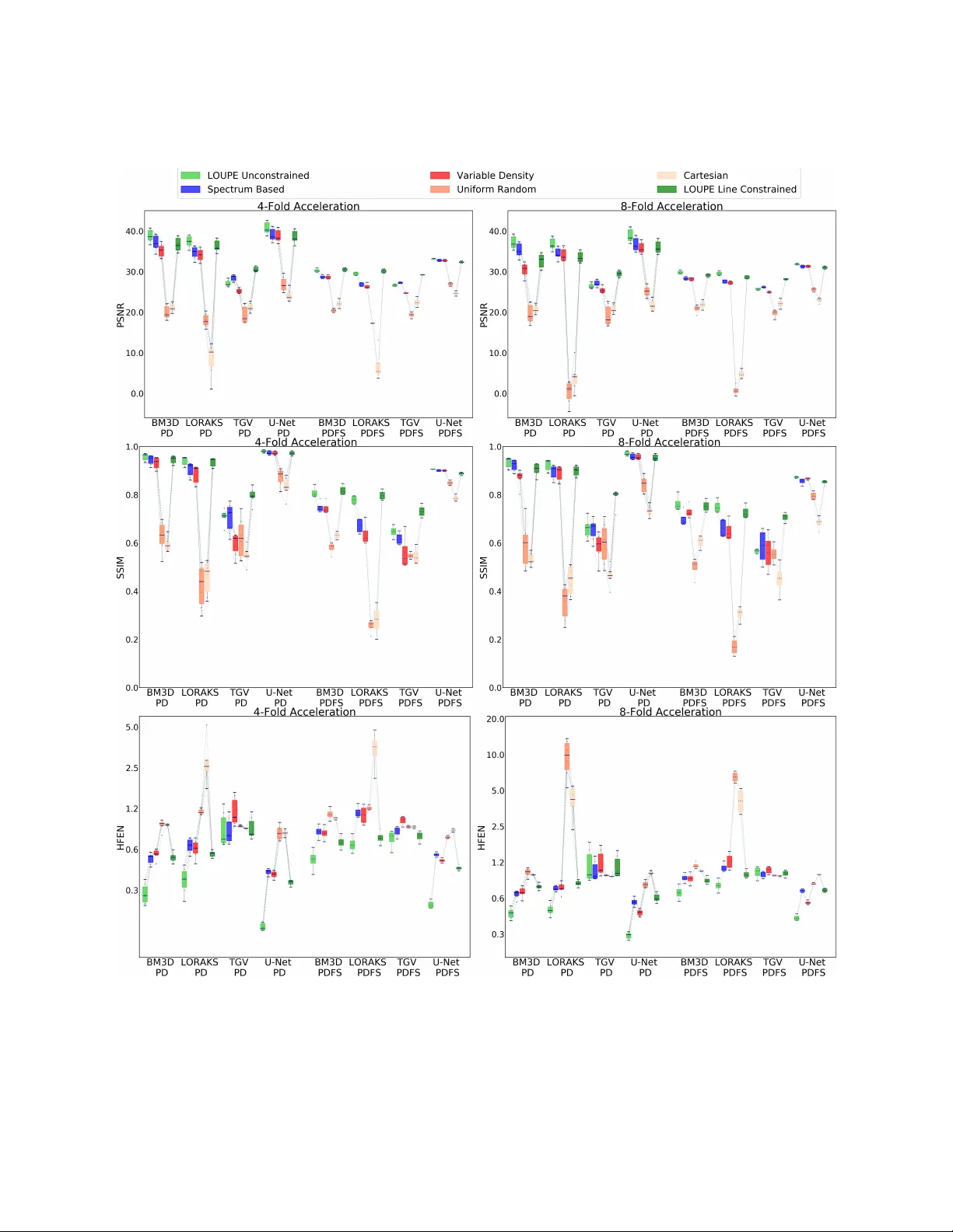
1 Deep-lear ning-based Optimization of the Under -sampling Patter n in MRI Cagla D. Bahadir*, Alan Q. W ang*, Adrian V . Dalca, and Mert R. Sabuncu In compressed sensing MRI (CS-MRI), k-space measur ements are under -sampled to achieve accelerated scan times. CS-MRI presents two fundamental problems: (1) where to sample and (2) how to reconstruct an under-sampled scan. In this paper , we tackle both problems simultaneously f or the specific case of 2D Cartesian sampling, using a novel end-to-end learning framework that we call LOUPE (Learning-based Optimization of the Under -sampling PattErn). Our method trains a neural network model on a set of full-resolution MRI scans, which are retr ospectively under -sampled on a 2D Cartesian grid and forwarded to an anti-aliasing (a.k.a. reconstruction) model that computes a r econstruction, which is in turn compared with the input. This f ormulation enables a data-driv en optimized under- sampling pattern at a given sparsity le vel. In our experiments, we demonstrate that LOUPE-optimized under-sampling masks are data-dependent, varying significantly with the imaged anatomy , and perform well with different reconstruction methods. W e present empirical results obtained with a large-scale, publicly av ailable knee MRI dataset, where LOUPE offered superior reconstruction quality across different conditions. Even with an aggressi ve 8-f old acceleration rate, LOUPE’s reconstructions contained much of the anatomical detail that was missed by alternativ e masks and r econstruction methods. Our experiments also show how LOUPE yielded optimal under-sampling patterns that were significantly different f or brain vs knee MRI scans. Our code is made fr eely a vailable at https://github .com/cagladbahadir/ LOUPE/. Index T erms —Compressed Sensing, Magnetic Resonance Imaging, Deep Learning I . I N T R O D U C T I O N M A GNETIC Resonance Imaging (MRI) is a ubiquitous, non-in vasi ve, and versatile biomedical imaging tech- nology . A central challenge in MRI is long scan times, which constrains accessibility and leads to high costs. One remedy is to accelerate MRI via compressed sensing [1], [2]. In com- pressed sensing MRI, k-space data (i.e., the Fourier transform of the image) is sampled belo w the Nyquist-Shannon rate [1], which is often referred to as “under-sampling. ” Given an under-sampled set of measurements, the objective is to “recon- struct” the full-resolution MRI. This is the main problem that most of the compressed sensing literature is focused on and is con ventionally formulated as an optimization problem that trades of f two objectiv es: one that quantifies the fit between the measurements and the reconstruction (sometimes referred to as Cagla D. Bahadir and Mert R. Sabuncu are with the Meinig School of Biomedical Engineering, Cornell Univ ersity . Alan Q. W ang and Mert R. Sabuncu are with the School of Electrical and Computer Engineering, Cornell University . Adrian V . Dalca is with the Computer Science and Artificial Intelligence Lab at the Massachusetts Institute of T echnology and the A.A. Martinos Center for Biomedical Imaging at the Massachusetts General Hospital. * indicates equal contribution. Cagla D. Bahadir and Alan Q. W ang are co-first authors. data consistency), and another that captures prior knowledge on the distrib ution of MRI data. This latter objecti ve is often achiev ed via the incorporation of regularization terms, such as the total v ariation penalty and/or a sparsity-inducing norm on transformation coefficients, like wav elets or a dictionary decomposition [3]. Such regularization functions aim to cap- ture different properties of real-world MR images, which in turn help the ill-posed reconstruction problem by guiding to more realistic solutions. One approach to de velop a data-dri ven regularization function is to construct a sparsifying dictionary , for example, based on image patches [4]–[6]. Once the optimization problem is set up, the reconstruction algorithm often iterati vely minimizes the re gularization term(s) and enforces data consistency in k-space. This is classically solved for each acquired dataset, independently , and from scratch - a process that can be computationally demanding. As we describe in the following section, there has been a recent surge in machine learning based methods that take a different, and often computationally more efficient approach to solving the reconstruction problem. These techniques are gradually becoming more widespread and expected to com- plement existing regularized optimization based approaches. Another critical component of compressed sensing MRI is the under-sampling pattern. For a giv en acceleration rate, there is an exponentially large number of possible patterns one can implement for under-sampling. Each of these under-sampling patterns will in general lead to different reconstruction per- formance that will depend on the statistics of the data and the utilized reconstruction method. One way to view this is to regard the reconstruction model as imputing the parts of the Fourier spectrum that was not sampled. For example, a frequency component that is constant for all possible datasets we might observe, does not need to be sampled when we use a reconstruction model that can lev erage this information. On the other hand, highly v ariable parts of the spectrum will likely need to be measured to achie ve accurate reconstructions. This simple vie wpoint ignores the potentially multi-v ariate nature of the distribution of k-space measurements. For instance, miss- ing parts of the Fourier spectrum might be reliably imputed from other acquired parts, due to strong statistical dependency . W idely used under-sampling strategies in compressed sensing MRI include Random Uniform [2], V ariable Density [7] and equi-spaced Cartesian [8] with skipped lines. These tech- niques, howe ver , are often implemented heuristically , not in a data-driven adapti ve fashion, and their popularity is largely due to their ease of implementation and good performance when coupled with popular reconstruction methods. As we discuss below , some recent ef forts compute optimized under- sampling patterns - a literature that is closely related to our 2 primary objectiv e. In this paper , we propose to merge the two core problems of compressed sensing MRI: (1) optimizing the under-sampling pattern and (2) reconstruction. W e consider these two prob- lems simultaneously because they are closely inter-related. Specifically , the optimal under-sampling pattern should, in general, depend on the reconstruction method and vice versa. Inspired by recent dev elopments in machine learning, we propose a nov el end-to-end deep learning strategy to solve the combined problem. W e call our method LOUPE, which stands for Learning-based Optimization of the Under-sampling PattErn. A preliminary version of LOUPE was published as a conference paper [9]. In this journal paper, we present an extended treatment of the literature, an important modification to the LOUPE objectiv e that enables us to directly set the desired sparsity lev el while obviating the need to identify the value of an extra hyper-parameter , more details on the methods, and new experimental results. The rest of the paper is organized as follows. In the fol- lowing two sections, we revie w two closely related bodies of work: a rapidly growing list of recent papers that use machine learning for ef ficient and accurate reconstruction; and sev eral proposed approaches to optimize the under -sampling pattern. Section IV then presents the mathematical and implementation details of the proposed method, LOUPE. Section V presents our experiments, where we compare the performance obtained with sev eral benchmark reconstruction methods and under- sampling patterns. Section VI concludes with a discussion. I I . M A C H I N E L E A R N I N G F O R U N D E R - S A M P L E D I M A G E R E C O N S T RU C T I O N Over the last few years, machine learning methods have been increasingly used for medical image reconstruction [10]– [15], including compressed sensing MRI. An earlier exam- ple is the Bayesian non-parametric dictionary learning ap- proach [16]. In this framework, dictionary learning is used in the reconstruction problem to obtain a regularization objectiv e that is customized to the image at hand. The reconstruction problem is solved via a traditional optimization approach. More recently , fueled by the success of deep learning, sev eral machine learning techniques ha ve been proposed to implement efficient and accurate reconstruction models. For instance, in a high profile paper, Zhu et al. demonstrated a ver- satile supervised learning approach, called A UTOMAP [13]. This method uses a neural network model to map sensor mea- surements directly to reconstruction images, via a manifold representation. The e xperimental results sho w that A UTOMAP can produce high quality reconstructions that are robust to noise and other artifacts. Another machine learning based reconstruction approach in volves using a neural network to efficiently ex ecute the iterations of the Alternating Direction Method of Multipliers (ADMM) method that solves a conv en- tional optimization problem [10], [17]. This technique, called ADDM-Net, uses an “unrolled” neural network architecture to implement the iterativ e optimization procedure. In a similar approach, an unrolled neural network is used to implement the iterations of the Landweber method [15]. Another class of methods rely on the U-Net architecture [18] or its variants. For example U-Net-like models have been trained in a supervised fashion to remove aliasing artifacts in the imaging domain [19], [20]. The U-Net architecture has also been used by appending with a forward physics based model to learn phase masks for depth estimation in other computer vision applications [21]. In these methods, the neural network takes as input a poor quality reconstruction (e.g., obtained via a simple in verse Fourier transform applied to zero-filled k-space data) to compute a high quality output, where the objective is to minimize the loss function (e.g., squared difference) between the output and the ground truth provided during training. Inspired by the success of Generative Adversarial Networks (GANs) [22], several groups hav e proposed the use of an adversarial loss, in addition to the more con ventional loss functions, to obtain better quality reconstructions [23]–[26]. The method we propose in this paper b uilds on the neural net-based reconstruction framew ork, which of fers a compu- tationally efficient and differentiable anti-aliasing model. W e combine the anti-aliasing model with a retrospecti ve under- sampling module, and learn both blocks simultaneously . I I I . D A TA - D R I V E N U N D E R - S A M P L I N G I N C O M P R E S S E D S E N S I N G M R I The under-sampling pattern in k-space is closely related to reconstruction performance. Several under-sampling patterns are widely used, including Random Uniform [2], V ariable Density [7], [27] and equi-spaced Cartesian [8] with skipped lines. Since the early work by Lustig et al. [27], random or stochastic under-sampling strategies are commonly used, as they induce noise-like artifacts that are often easier to remov e during reconstruction. Ho we ver , as several papers ha ve pointed out, the quality of reconstruction can also be improved by adapting the under-sampling pattern to the data and applica- tion. W e underscore that there is a related, but more general problem of optimizing projections in compressed sensing, which has receiv ed considerable attention [28]–[31]. Below , we revie w adaptive under-sampling strategies in compressed sensing MRI, which is the focus of our paper . Knoll et al. proposed an under-sampling strategy that fol- lows the power spectrum of a provided example (template) image [32]. This method collects denser samples in parts of k-space that has most of the power concentrated, such as the low-frequenc y components of real-world MRIs. The authors argue that most of the anatomical variability is reflected in the phase and not magnitude of the Fourier spectrum, justifying the decision to rely on the magnitude to construct the under- sampling pattern. In experiments, they apply their method to both knee and brain MRI scans, demonstrating better performance than parametric variable density under-sampling patterns [27]. Kumar Anand et al. presented a second-order cone op- timization technique for finding the optimal under-sampling trajectory in volumetric MRI scans [33]. Their heuristic strat- egy accounts for cov erage, hardware limitations and signal generation in a single con vex optimization problem. Building on this approach, Curtis et al. employed a genetic algorithm 3 to optimize sampling trajectories in k-space, while accounting for multi-coil configurations [34]. Seeger et al. employed a Bayesian inference approach to optimize Cartesian and spiral trajectories [35]. Their iterative, greedy technique seeks the under-sampling pattern in k-space that minimizes the uncertainty in the computed reconstruction, conditioned on the acquired measurements. In a recent paper that explores a similar direction, Haldar et al. proposed a new framework called Oracle-based Experiment Design for Imaging Parsimoniously Under Sparsity constraints (OEDI- PUS) [36]. OEDIPUS solves an integer programming problem to minimize a lo wer (Cramer -Rao) bound on the v ariance of the reconstruction. Roman et al. offered a novel theoretical perspective on compressed sensing, which underscores the importance of adapting the under-sampling strategy to the structure in the data [37]. The authors also presented an innovati ve multilev el sampling approach that depends on the resolution and the structure of the data that empirically outperforms competing under-sampling schemes. An alternativ e class of data-driven approaches aims to find the optimal under-sampling pattern that yields the best re- construction or imputation quality , using some full-resolution training data that is retrospectively under-sampled [38]. The central challenge in this framework is to efficiently solve two computationally challenging nested optimization prob- lems. The first, outer problem is to identify the optimal under-sampling mask or sampling trajectory that achieves best reconstruction quality , which is in turn the result of an inner optimization step. Several authors have proposed to solve this nested pair of problems via heuristic, greedy algorithms [39]–[43]. In an empirical study , Zijlstra et al. demonstrated that a data-driven optimization approach [40], [44] can yield better reconstructions than those obtained with more conv entional methods [27], [32]. Howe ver , prior data- driv en methods mostly lack the computational efficiency to handle large-scale full-resolution (training) data. Furthermore, they are often not flexible enough to deal with different types of under-sampling schemes. In this paper , we present a novel, flexible, and computa- tionally ef ficient data-driven approach to optimize the under- sampling pattern. Instead of formulating the problem as two nested optimization problems, we leverage modern machine learning techniques and take an end-to-end learning perspec- tiv e. Similar to recent deep learning based reconstruction tech- niques [19], [20], our implementation employs the U-Net [18] architecture, which we append with a probabilistic under- sampling step that is also learned. W e assume we are pro- vided with full-resolution MRI data, which we retrospecti vely under-sample. W e note that there hav e been contemporaneous efforts [45]–[47] that build on our prior work [9] to take a deep learning-based approach similar to ours for optimizing the under-sampling pattern in compressed sensing. I V . M E T H O D A. Learning-based Optimization of Under-sampling P attern LOUPE solves the two problems of compressed sensing simultaneously: (1) identifying the optimal under-sampling pattern; and (2) reconstructing from the under-sampled mea- surements. Building on stochastic strategies of compressed sensing, we consider a probabilistic mask P , which describes an independent Bernoulli random v ariable at each k-space point. The probabilistic mask P is defined on the full- resolution k-space grid, and at each point takes on non- negati ve continuous probability values, i.e., P ∈ [0 , 1] d , where d is the total number of grid points. For example, for a 100 × 100 image, d = 10 , 000 . W e parameterize P with an unconstrained image O ∈ R d , such that P = σ t ( O ) . Here, σ t denotes an element-wise sigmoid, with slope t , which is treated as a hyper-parameter . P i = 1 1+ e − t O i , where the sub- script i index es the grid points. Binary realizations drawn from P represent an under-sampling mask M ∈ { 0 , 1 } d : i.e., M ∼ Q d i =1 B ( P i ) , where B ( p ) denotes a Bernoulli random variable with parameter p . The binary mask M has value 1 for grid points that are acquired and 0 for points that were not acquired. Suppose we are provided with a collection of complex- valued full-resolution images, denoted as { x j ∈ C d } n j =1 , where j corresponds to the scan number and n is the total number of scans. In our following treatment, without loss of generality , we will assume the pro vided data are in image domain. This can be modified to accept raw k-space measure- ments, by simply removing a forward Fourier transform. In the LOUPE framework, we solve the following problem: min O ,θ E M ∼ Q i =1 B ( σ t ( O i )) n X j =1 k A θ ( F H diag ( M ) F x j ) − x j k 2 2 , such that 1 d k σ t ( O ) k 1 = α (1) where F ∈ C d × d stands for the (forward) Fourier transform matrix, F H is the in verse Fourier transform matrix, A θ denotes an anti-aliasing reconstruction function parameterized with θ , k·k 2 denotes the L2 norm, k·k 1 denotes the L1 norm, α ∈ [0 , 1] is the desired sparsity level, and diag ( · ) denotes a diagonal matrix obtained by setting the diagonal to the argument vector . The loss function of Equation (1) quantifies the a verage quality of the reconstruction. The constraint 1 d k σ t ( O ) k 1 = 1 d k P k 1 = α ensures that the probabilistic under-sampling mask has an av erage value of α , which will correspond to an acceleration factor of R = 1 /α . W e emphasize that the problem formula- tion of Equation (1) is slightly different than the formulation in our conference paper [9], where we employed a sparsity inducing regularization instead of a hard constraint. That formulation required fine-tuning a hyper -parameter in order to obtain the desired sparsity le vel, which was computationally inefficient. In this paper we implement a practical strategy , described belo w , to solve the problem with the hard sparsity constraint directly . The loss function in v olves an expectation over the random binary mask M . W e approximate this expectation using a 4 Monte Carlo-based sample averaging strategy: min O ,θ n X j =1 1 K K X k =1 k A θ ( F H diag ( m ( k ) ) F x j ) − x j k 2 2 , such that 1 d k σ t ( O ) k 1 = α (2) where m ( k ) are independent realizations drawn from Q i B ( σ t ( O i )) . Similar to the re-parameterization trick used in variational techniques, such as the V AE [48], we can re- write Equation (2): min O ,θ n X j =1 1 K K X k =1 k A θ ( F H diag ( U ( k ) ≤ σ t ( O )) F x j ) − x j k 2 2 , such that 1 d k σ t ( O ) k 1 = α (3) where U ( k ) are independent realizations drawn from Q d i =1 U (0 , 1) , a spatially independent set of uniform random variables on [0 , 1] . The result of the inequality operation is 1 if the condition is satisfied and 0 otherwise. In Equation (3) the random draws are thus from a constant distribution (inde- pendent uniform) and the probabilistic mask P (through its parameterization O ), only ef fects the thresholding operation. B. Implementation In our first version of LOUPE, we used a 2D U-Net architecture [18] for the anti-aliasing function, as depicted in Figure 1 and similar to other prior work [19], [20]. T o enable a differentiable loss function, we relaxed the non-differentiable threshold operation of Equation (3) with a sigmoid. This relax- ation is similar to the one used in recent Gumbel-softmax [49] and concrete distrib utions [50] in training neural netw orks with discrete representations. Our final objective is: min O ,θ n X j =1 1 K K X k =1 k A θ ( F H diag ( σ s ( σ t ( O ) − U ( k ) )) F x j ) − x j k 2 2 , such that 1 d k σ t ( O ) k 1 = α (4) where σ s ( a ) = 1 1+ e − sa is a sigmoid with slope s . A critical issue for LOUPE is the enforcement of the hard constraint 1 d k σ t ( O ) k 1 = 1 d k P k 1 = α . T o achieve this we introduce a normalization layer , which rescales P to satisfy the constraint. W e first define ¯ p = k P k 1 d , which is the av erage value of the pre-normalization probabilistic mask. Note that 1 − ¯ p is the av erage value of 1 − k P k 1 . W e define the normalization layer as: N α ( P ) = ( α ¯ p P , if ¯ p ≥ α 1 − 1 − α 1 − ¯ p ( 1 − P ) , otherwise. (5) It can be shown that Equation (5) yields N α ( P ) ∈ [0 , 1] d and k N α ( P ) k 1 d = α . This normalization trick allows us to con vert the constrained problem of Equation (4) to the following unconstrained problem: min O ,θ n X j =1 1 K K X k =1 k A θ ( F H diag ( σ s ( N α ( σ t ( O )) − U ( k ) )) F x j ) − x j k 2 2 . (6) Figure 1 illustrates an instantiation of the LOUPE model. In the depicted version of LOUPE, we used a U-Net archi- tecture to implement A θ , the reconstruction network. W e have also experimented with an alternativ e reconstruction model, namely Cascade-Net proposed in [51]. In the supplementary material, we present LOUPE results obtained with this alter - nativ e implementation. The LOUPE network accepts complex 2D images represented as two channels, corresponding to the imaginary and real components. The network applies a forward discrete Fourier transform, F , conv erting the data into k-space. The k-space measurements are under-sampled by ˜ m = σ s ( P − u ( k ) ) , which approximates a Monte Carlo realization of the probabilistic mask P . The v alues of the probabilistic mask are computed using the sigmoid operation of pixel-wise parameters O that are learned during the training process. The mask ˜ m is multiplied element-wise with the k-space data (approximating retrospectiv e under -sampling by inserting zeros at missing points), which is then passed to an in verse discrete Fourier transform F H . This image, which will typically contain aliasing artifacts, is then provided as input to the anti-aliasing network A θ ( · ) , also called the reconstruction network. This network takes a complex-v alued under-sampled image, represented as two- channels, and aims to minimize the reconstruction error, such as the squared difference between the magnitude images of ground truth and the reconstruction. W e can view the entire pipeline to be made up of two building blocks: the first optimizing the under-sampling pattern, and the second solving the reconstruction problem. The model was implemented in Keras [52], with T ensor- flow [53] in the back-end. Custom functions were adapted from the Neuron library [54]. AD AM [55] with an initial learn- ing rate of 0 . 001 was used for optimization, and learning was terminated when validation loss plateaued. Consistent with prior work [48]–[50], a single Monte Carlo realization was drawn for each training datapoint. This is common practice in variational neural networks as it is a computationally ef ficient approach that yields an unbiased estimate of the gradient that is used in stochastic gradient descent. W e used a batch size of 16. W e used a slope value of s = 200 for σ s that approximates the thresholding operation and a slope value of t = 5 for σ t that squashes the values of O to the range [0 , 1] . These values for the slope hyper-parameters were chosen based on a grid search strategy , where we identified the pair of values that yields the smallest validation loss (see Supplementary Material). W e note, ho wev er, that we did not observe a significant amount of sensitivity to these values. Our code is freely a v ailable at: https://github .com/cagladbahadir/LOUPE/ 5 Fig. 1. LOUPE architecture with two b uilding blocks: The Under-sampling Pattern Optimization Network and the Anti-aliasing Network. The model implements an end-to-end learning framework for optimizing the under-sampling pattern while learning the parameters for faithful reconstructions. The normalization layer for the probabilistic mask computes Equation (5). Red arro ws denote 2D conv olutional layers with a kernel size of 3 × 3 , followed by Leaky ReLU activ ation and Batch Normalization. Green vertical arro ws represent av erage pooling operations and yellow vertical arrows refer to up-sampling. The initial number of channels in the U-Net is 64 , which doubles after each average pooling layer. The U-Net also uses skip connections depicted with gray horizontal arrows, that concatenate the corresponding layers to facilitate better information flo w through the network. V . E M P I R I C A L A N A L Y S I S A. Data W e conducted our experiments using the NYU fastMRI dataset [56] (fastmri.med.nyu.edu). This is a freely a v ailable, large-scale, public data set of knee MRI scans. The dataset originally comprises of 2D coronal knee scans acquired with two pulse sequences that result with Proton Density (PD) and Proton Density Fat Supressed (PDFS) weighted images. In our experiments, we used the provided emulated single-coil (ESC) k-space data from the Biograph mMR (3T) scanner , which were derived from raw 15-channel multi-coil data. W e used 100 volumes from the provided official training dataset as our training dataset, and split the provided v alidation data into two halves, where we used 10 volumes for v alidation and 10 volumes for test. W e could not rely on the provided test data for ev aluation as they were not fully sampled. For the scans we analyzed, the sequence parameters were: echo train length of 4, matrix size of 320x320, in plane resolution of 0 . 5 mm × 0 . 5 mm , slice thickness of 3 mm and no gap between slices. The time of repetition (TR) varied between 2200 and 3000 ms and the Echo T ime (TE) ranged between 27 and 34 ms . T raining volumes had 38 ± 4 slices, where the validation volumes had 37 ± 3 and test volumes had 38 ± 4 . Each set (training, validation and test) had differing slice sizes across volumes. After taking the Inv erse Fourier Trans- form of the ESC k-space data, and rotating and flipping the images to match the orientation in the fastMRI paper [56], we cropped the central 320x320 and normalized by dividing to the maximum magnitude within each v olume. The U-Net architecture we emplo yed was also used in the original NYU fastMRI study [56] for reconstruction, with the only difference that their implementation accepted a single- channel, real-valued input image. B. Evaluation W e used three metrics in the quantitativ e e v aluations of the reconstructions with respect to the ground truth images created from fully sampled measurements: (1) peak signal to noise ratio (PSNR), (2) structural similarity index (SSIM), and (3) high frequency error norm (HFEN). PSNR is a widely used metric for ev aluating the quality of reconstructions in compressed sensing applications [10], [57], defined as: PSNR( x , ˆ x ) = 10 log 10 max( x ) 2 d k x − ˆ x k 2 2 , (7) where d is, as above, the total number of pixels in the full- resolution grid, and ˆ x denotes the reconstruction of the ground truth full-resolution image x . 6 SSIM aims to quantify the percei ved image quality [58]: SSIM( x , ˆ x ) = (2 µ x µ ˆ x + c 1 ) + (2 σ x ˆ x + c 2 ) ( µ 2 x + µ 2 ˆ x + c 1 )( σ 2 x + σ 2 ˆ x + c 2 ) , (8) where µ x and µ ˆ x are defined as the “local” av erage values for the original and reconstruction images, respecti vely , computed within an N × N neighborhood. Similarly , σ 2 x and σ 2 ˆ x are the local v ariances; and σ x ˆ x is local cov ariance between the reconstruction and ground truth images. c 1 = ( k 1 L ) 2 and c 2 = ( k 2 L ) 2 are constants that numerically stabilize the division, where L is the dynamic range of the pixel values and k 1 and k 2 are user defined. W e use the parameters provided in [56] for computing SSIM values: k 1 = 0 . 01 , k 2 = 0 . 03 , and a window size of 7 × 7 . The dynamic range of pixel values was computed over the entire volume. Finally , we also report the high-frequency error norm (HFEN), which is used to quantify the quality of reconstruc- tion of edges and fine features. F ollo wing [5], we use a 15 × 15 Laplacian of Gaussian (LoG) filter with a standard deviation of 1 . 5 pix els. The HFEN is then computed as the L2 difference between LoG filtered ground truth and reconstruction images. C. Benchmarks W e compared the LOUPE-optimized mask and other mask configurations, together with one machine learning (ML) based and three non-ML based reconstruction techniques. 1) Reconstruction Methods Each reconstruction method was optimized on a represen- tativ e slice from the data-set to find the values of hyper- parameters that yielded the best quality reconstruction for each of the individual masks. In other words, hyper-parameter tuning was done separately for each mask. The first benchmark reconstruction method is BM3D [59], which is an iterativ e algorithm that alternates between de- noising and reconstructions steps, and was shown to yield faithful reconstructions in the under-sampled cases. 1 A grid search on the parameters: σ , noise and λ were conducted, ov er the range 3 − 3 × 10 2 and 0 − 10 2 , respectiv ely . The second reconstruction benchmark method, called P- LORAKS, is based on lo w-rank modeling of local k-space neighborhoods [60], [61]. 2 A grid search on the parameters: λ , VCC (V irtual Conjugate Coils) and rank was conducted. The regularization parameter λ was searched between 10 − 2 and 1. The rank value which is related to the non-conv e x regularization penalty was searched between 1 to 45 and the VCC, which is a Boolean parameter was searched for both cases: 1 and 0. The third benchmark method is T otal Generalized V ariation (TGV) based reconstruction with Shearlet Transform [62]. The method regularizes image regions while keeping the edge information intact. 3 W e conducted a grid search for the parameters β , λ , α 0 , α 1 and µ 1 , adopting a range for each parameter based on the suggestions from the original 1 W e used the code at: http://web .itu.edu.tr/eksioglue/pubs/BM3D MRI.htm. 2 W e used the code available at: https://mr .usc.edu/download/loraks2/. 3 W e used the code at http://www .math.ucla.edu/ ∼ wotaoyin/papers/tgv shearlet.html. paper [62]. λ was searched between 10 − 3 and 5 × 10 − 1 , β was searched between 10 2 and 10 3 . The parameters µ 1 , α 0 and α 1 were respectiv ely searched between values: 3 × 10 2 and 10 × 3 , 8 × 10 − 4 to 10 − 2 and 10 − 3 to 10 − 1 . The final benchmark reconstruction method is the residual U-Net [19], which is also a building block in our model. In this framew ork, the U-Net is used as an anti-aliasing neural net- work widely used for biomedical image applications. Unlike in LOUPE, the benchmark U-Net implementation is trained for a fixed under-sampling mask, that is provided by the user . In our experiments the U-Net models were individually trained and tested for each mask configuration. 2) Under-sampling Masks W e implemented sev eral widely used benchmark under- sampling masks, sho wn in Figure 2. The first set of masks we considered are what we refer to as 2D Cartesian under- sampling masks. These are physically feasible for 2D imaging with (i) two phase-encoding dimensions and no frequency- encoding gradient; or (ii) for 3D acquisition with one fre- quency encoding dimension and two phase-encoding dimen- sions. In this category , we have “Random Uniform” [2], which e xhibits the benefits of stochastic under -sampling in creating incoherent, noise-like artifacts [1], thus facilitating the discrimination of artifacts from the signal present in the image. W e also employed a parametric V ariable Density [7] (VD) mask that samples lower frequencies more densely , while still enjoying the benefits of creating noise-like artifacts. W e used the publicly av ailable code of [27] to identify the optimal v alues of the VD mask that maximizes incoherence (of aliasing artifacts) in the wavelet domain. Another 2D under- sampling mask we implemented was a data-driven strategy that was based on [63]. In our implementation, we av eraged the magnitude spectrum of all the fully-sampled training data. The av erage spectrum was then thresholded to keep the k- space points that ha ve the largest average magnitude. W e refer to this mask as “spectrum-based. ” Next, we considered 1D under-sampling masks, which are physically feasible for 2D imaging with one frequency- encoding dimension and one phase-encoding dimension. Cartesian [8] with skipped lines orthogonal to the provided read-out direction is a popular mask in this category . In addition, we implemented a version of LOUPE where the mask was constrained to be made up of lines along the read- out direction, which is similar to a strate gy proposed in [45]. W e achieved this with a simple modification in our code by sharing the weights corresponding to the entries of O along each read-out line. This “line-constrained version” of LOUPE, we believ e, is one step closer to being physically realistic. When we need to be explicit, we refer to the first LOUPE version as unconstrained. W e underscore that it might not be fair to compare the 1D and 2D under-sampling masks, as the two categories would rely on different acquisition protocols. Thus, any comparisons we present below need to account for this dif ference. D. Results Figure 2 shows the LOUPE optimized and benchmark masks, for two different acceleration rates R = 4 and R = 8 . 7 Fig. 2. LOUPE-optimized and benchmark masks for two le vels of acceleration rates for NYU fastMRI data set: R = 4 and R = 8 . Black dots represent k-space points that are sampled and white areas correspond to measurements that are not acquired. The two right-most masks represent 1D under -sampling strategies, whereas the remaining four represent 2D under-sampling. These two categories of under-sampling rely on different acquisition protocols. The LOUPE, spectrum-based, and variable density masks share the behavior of a drop in density from lower to higher frequencies, howe ver differ significantly in their symmetry and shape. Although the unconstrained LOUPE-optimized masks are similar to the VD masks in terms of emphasizing lower frequencies, importantly lateral frequencies are fav ored significantly more than ventral/dorsal frequencies. The data- driv en spectrum-based masks, on the other hand, exhibit a similar tendency to pick out more lateral frequencies, yet with a dramatically dif ferent overall shape that concentrates around the two ax es. The line-constrained LOUPE masks also show a strong preference for lower frequencies. In an earlier conference paper [9], we had reported an unconstrained LOUPE-optimized mask for T1-weighted brain MRI scans, obtained from a public dataset [64]. Figure 3 shows a side by side comparison of the two LOUPE-optimized masks for the knee and brain anatomies, respectiv ely , em- phasizing the asymmetry present in the knee dataset. The knee mask fav ors lateral frequencies more than ventral/dorsal frequencies due to the unique features of knee anatomy , where there is significantly more tissue contrast in the lateral direction. Brain scans, on the other hand, exhibit a more radially symmetric behavior . This comparison highlights the importance of a data-driven approach in identifying the under- sampling mask. Figure 4 shows subject-lev el quantitative reconstruction quality values computed for the different masks and recon- struction methods, under two different acceleration conditions. W e present the results for the 6 test subjects with PD weighted images and 4 test subjects with PDFS weighted images, separately . The fat suppression operation inherently lowers the signal lev el, as fat has the highest levels of signal in an MRI scan, thus yielding a noisier image, where small details are more apparent. In contrast, regular PD weighted scans that contain fat tissue ha ve inherently higher SNR. Therefore, the PD scans yield better quality reconstructions compared to the PDFS scans. Figure 4 re v eals that o verall LOUPE yields significantly better results than competing masks, when used with an y of the tested reconstruction methods and under the two acceleration rates. Furthermore, the U-Net reconstruction model, coupled Fig. 3. LOUPE-optimized under-sampling masks (for R = 8 ) compared side by side for the knee and brain anatomies. The brain mask was deriv ed using the data described in our prior work [9]. There is a striking difference in the symmetry , which can be appreciated visually . Note that black dots represent k-space points that are sampled and white areas correspond to measurements that are not acquired. with LOUPE-optimized masks yields the best reconstructions, for both acceleration rates and for all test subjects. Unsur- prisingly , the unconstrained version of LOUPE is generally better than the line-constrained version, with the exception of the TGV reconstruction method, where the line-constrained LOUPE outperformed unconstrained LOUPE. These results suggest that LOUPE-optimized masks can offer a performance gain e ven when not used with the U-Net based reconstruction method. W e further observe that the V ariable Density and spectrum-based masks outperforms the uniform mask, which is consistent with prior literature. T able I lists the summary quantitativ e values for each of 8 the reconstruction method and mask configurations, where av erages within the PD and PDFS subjects are presented separately . Supplementary T ables 1 and 2 includes standard de- viations for these results. The lowest HFEN and highest PSNR and SSIM values are bolded for each reconstruction method, metric and subject group. W e observe that the LOUPE- optimized masks yield the highest reconstruction quality under all considered conditions, and the line-constrained and uncon- strained versions are often quite similar . For reference, we also added the best v alues reported in [56] that was achieved with a U-Net reconstruction model and a V ariable Density Cartesian mask. W e underscore that their model was trained on the full training set and ev aluated on the full validation set. Ne vertheless, we observe that their results are consistent with ours, often falling between our U-Net models trained for Cartesian and VD masks, b ut alw ays under -performing compared to the U-Net model trained with LOUPE masks. Figures 5 and 6 show example PD weighted slices and U-Net based reconstructions, obtained after under-sampling with R = 4 and R = 8 , using different masks. As can be appreciated from these figures, much of the structural details that correspond to the femur , tibia, tendons, ligaments, muscle tissue, and meniscus are more faithfully captured in the reconstructions obtained with the LOUPE-optimized masks, whereas reconstructions computed with other masks were more blurry . For example, edges of the posterior cruciate ligament and lateral meniscus suf fer from blurring artifacts in the benchmark mask configurations compared to the LOUPE- optimized masks. Overall, in agreement with the quantitativ e results presented abov e, the LOUPE-optimized mask yields the best-looking reconstruction results and these reconstructions appear less prone to artifacts and blurring, while preserving more of the anatomical detail. In the Supplementary Material, we present our results obtained with a version of LOUPE where the U-Net recon- struction model was replaced with Cascade-Net [51] with the same architecture details of the reference paper . Everything else in LOUPE, including all optimization settings were kept the same. W e observe that the optimized masks are very similar between U-Net-LOUPE and Cascade-Net-LOUPE. W e also quantified the quality of reconstructions with these masks and found that there was no substantial difference. These results, we believ e, demonstrate that LOUPE can be relatively robust to the choice of the reconstruction architecture. W e note, howe ver , that we ha ve not experimented with more adv anced reconstruction networks, such as the recently proposed [65], which might yield different results. W e consider the explo- ration of different architectural designs for LOUPE as an important direction for future research. V I . D I S C U S S I O N Compressed sensing is a promising approach to accelerate MRI and make the technology more accessible and affordable. Since its introduction ov er a decade ago, it has gained in popularity and been used in a range of application domains. Compressed sensing MRI has two fundamental challenges. The first is identifying where in k-space to sample (acquire) from. One approach to solve this problem is to take a data- driv en strategy , where the optimal under-sampling pattern is identified using, for example, a collection of full-resolution scans that are retrospecti vely under-sampled. The second core problem of compressed sensing MRI is solving the ill-posed in verse problem of reconstructing a high quality image from under-sampled measurements. This is con ventionally solved via a regularized optimization approach, and more recently deep learning techniques ha ve been proposed to achie ve supe- rior performance. In this paper , we tackled both of these problems simultane- ously . W e leveraged recently proposed deep learning based reconstruction techniques to design an end-to-end learning technique that enabled us to optimize the under-sampling pattern on giv en training data. Our approach relies on full- resolution data that is under-sampled retrospectively , which is then fed to a reconstruction network. The final output is then compared to the original input to assess overall quality . W e formulate an objective that optimizes reconstruction quality with a constrained number of collected measurements. The stronger the constraint, the more aggressiv e acceleration rates we can achiev e. Our results indicate that LOUPE, the proposed method, can compute an optimized under-sampling pattern that is data-dependent and performs well with different reconstruc- tion methods. In this paper , we present empirical results obtained with a large-scale, publicly av ailable knee MRI dataset. Across all conditions we experimented with, LOUPE- optimized masks coupled with the U-Net based reconstruction model of fered the most superior reconstruction quality . Even with an aggressiv e 8-fold acceleration rate, LOUPE’ s recon- structions contained much of the anatomical detail that was missed by alternativ e masks as seen in Figure 6. In our primary experiments, we used a U-Net based recon- struction method in the implementation of LOUPE. Addition- ally , we in vestig ated the use of an alternativ e reconstruction network, namely Cascade-Net. Our results, which we present in the Supplementary Material, indicate that both versions of LOUPE achiev ed similar optimized masks and yielded similar reconstruction quality . Howe ver , we consider the exploration of dif ferent architectural designs (such as ADMM-Net [10] or MoDL [14]) for LOUPE as an important direction for future research. The LOUPE-optimized under-sampling mask for the ana- lyzed knee MRI scans exhibited an interesting asymmetric pattern, which emphasized higher frequencies along the lateral direction much more than those along the vertical direction. This is likely due the anisotropy in the field of view of sagittal knee images. This is in stark contrast to the LOUPE- optimized mask that we recently presented at a conference for T1-weighted brain MRI scans [9]. The brain mask exhibited a radially symmetric nature, very similar to a variable density mask, which is widely used in compressed sensing MRI. This comparison highlights the importance of adapting the under- sampling pattern to the data and application at hand. An important caveat of the presented LOUPE framework is that we largely ignored the costs of physically implement- ing the under-sampling pattern in an MR pulse sequence. 9 Fig. 4. Quantitative evaluation of reconstruction quality for the NYU fastMRI data set. T op: PSNR values (higher is better), middle: SSIM results (higher is better), bottom: high-frequency error norm (HFEN) results (lower is better). For each plot, we show four reconstruction methods using different acquisition masks, including LOUPE-optimized masks in green. Note that 2D (first four in each group) and 1D (last two in each group) under-sampling masks should be interpreted separately and any cross-category comparison should be done with caution. The slice-av eraged values for each test subject are connected with lines. For each box, the blue straight line shows the median value. Patients with Proton Density (PD) images and Proton Density Fat Suppressed (PDFS) images are shown separately . The whiskers indicate the the most extreme (non-outlier) data points. 10 Fig. 5. U-Net based reconstructions for an example PD slice from NYU fastMRI experiments with 4-fold acceleration rate ( α = 0 . 25 ). Each column corresponds to an under-sampling mask. Corresponding PSNR values are listed above each image. Fig. 6. U-Net based reconstructions for an example PD slice from NYU fastMRI experiments with 8-fold acceleration rate ( α = 0 . 125 ). Each column corresponds to an under-sampling mask. Corresponding PSNR values are listed above each image. In the unconstrained version of LOUPE, the cost of an under-sampling pattern is merely captured by the number of collected measurements. W e underscore that in 3D, the LOUPE-optimized mask can be implemented as a Cartesian trajectory , since the isolated measurement points in the coronal slices line up along the z-direction. W e also presented results for a readout-line-constrained version of LOUPE, which is consistent with widely used 2D acquisition protocols. These results, we believ e, demonstrate the utility and flexibility of LOUPE. Nonetheless, integrating the actual physical cost of a specific under-sampling pattern in an MR pulse sequence is a direction that we leave for future research. One way to achiev e this would be to constrain the sub-sampling mask to a class of viable trajectories, for example, by directly parameterizing those trajectories. Alternativ ely , one can incorporate sampling constraints that obey a set of predefined hardware requirements (as defined in terms of, e.g., peak currents and maximum slew rates of magnetic gradients), as described recently in [66]. Our paper restricted its treatment to Cartesian sampling and largely ignored non-Cartesian (off-the-grid) acquisition schemes, which can offer important benefits [67]–[69]. Ex- tension of LOUPE to non-Cartesian settings will inv olve the use of the non-uniform (in verse) Fourier transform operator or an approximation of it. Furthermore, one would need to interpolate off-grid measurements in retrospecti v e sampling. Another weakness of the presented LOUPE implementation is due to the relaxation of the thresholding operation, which allowed us to use a back-propagation-based learning strategy . Howe ver , due to this relaxation, the reconstruction model sees input data that have been rescaled with a continuous v alue between 0 and 1 . By adopting a relatively large slope pa- rameter ( s = 200 ), we ensure that these continuous values are almost always very close to zero or 1. Howe ver , this relaxation means that once we have obtained the optimized mask, we need to retrain a reconstruction model with a binary mask. Furthermore, we are likely paying a performance penalty due to the relaxation, since it will undoubtedly influence the optimization. W e see two ways to address this issue. The first approach is to implement the so-called “straight-through” gradient estimation strate gy , where the continuous relaxation is merely used in the backward pass for computing the gradient and not in the forward pass [70]. Another approach would in volve using non back-propagation based techniques, such as the REINFORCE estimator [71]. This technique is kno wn to suffer from high variance and there are se veral recent papers that hav e attempted to address this issue [72], [73]. W e plan to explore this direction in future work. In this paper , we used an L2 dif ference between the mag- nitude of the ground truth and reconstruction images to train LOUPE. Our experiments with an L2-loss computed on two- channel (complex-v alued) reconstructions produced inferior results. W e also noticed that our LOUPE-optimized masks did 11 not emphasize high frequency content, which can also explain some of the blurriness in reconstructions. This is particularly noticeable in the line-constrained LOUPE results. W e believ e that our choice of the L2 loss is the main cause of this effect, which can be remedied with alternate loss functions that care more about high-frequency content. W e note that we experimented with L1 reconstruction loss, as we reported in our conference paper [9]. Our experiments (results not shown) revealed that L1 loss can yield better quality results, particularly as measured by the high frequency error norm (HFEN). W e intend to explore such differences in future work. While these loss functions (L1 or L2) are a widely used global metrics of reconstruction quality , they might miss clinically important anatomical details. An alternative approach could be to devise loss functions that emphasize structural features that are relev ant to the clinical application. This is another future direction we will explore. In the current version of LOUPE, we did not consider parallel imaging via multiple coils. Such hardware-based tech- niques, in combination with compressed sensing, promise to yield even higher degrees of acceleration. Inv estigating how to combine LOUPE with multi-coil imaging will be an important area of research, as was recently demonstrated [74]. Finally , we would like to emphasize that LOUPE, as in any other data-driven optimization strategy , will perform sub- optimally if test time data differ significantly from training data. For example, if we train only on healthy subjects and then, at test time, are presented with pathological cases, the reconstructed scans might not be clinically useful. Thus, carefully monitoring reconstruction quality and ensuring the model is adapted to the new data will be of utmost importance in deploying this approach in the real world. For example, this could be achiev ed via fine-tuning the pre-trained LOUPE model on new data, as recently described in [75]. W e also consider machine learning paradigms that don’ t rely on high quality full-resolution data as an important direction. There hav e been some recent pre-prints in this domain [26], [76], [77]. Integrating such techniques into LOUPE will be critical for certain applications. For instance, in some anatomical regions such as the abdomen, a fully sampled scenario may not be possible due to organ motion, breathing, the cardiac cycle or other factors. This is also true for populations such as young children or patient groups, where subject motion can make the acquisition of high quality fully sampled data impossible. A C K N O W L E D G M E N T This work was, in part, supported by NIH R01 grants (R01LM012719 and R01A G053949, to MRS), the NSF Neu- roNex grant (1707312, to MRS), and an NSF CAREER grant (1748377, to MRS). This work was also in part supported by a Fulbright Scholarship (to CDB). Data used in the preparation of this article were obtained from the NYU fastMRI Initiativ e database [56]. As such, NYU fastMRI in vestigators provided data but did not par- ticipate in analysis or writing of this report. A listing of NYU fastMRI in vestig ators, subject to updates, can be found at:fastmri.med.nyu.edu. The primary goal of fastMRI is to test whether machine learning can aid in the reconstruction of medical images. The concepts and information presented in this paper are based on research results that are not commercially av ailable. Finally , we would like to express our gratitude for the extremely thorough, thoughtful, and constructiv e feedback we receiv ed from the Associate Editor Justin Haldar , and three anonymous revie wers. R E F E R E N C E S [1] M. Lustig, D. L. Donoho, J. M. Santos, and J. M. Pauly , “Compressed sensing MRI, ” IEEE signal processing magazine , vol. 25, no. 2, p. 72, 2008. [2] U. Gamper , P . Boesiger, and S. Kozerke, “Compressed sensing in dynamic MRI, ” Magnetic Resonance in Medicine , vol. 59, no. 2, pp. 365–373, 2008. [3] S. Ma, W . Yin, Y . Zhang, and A. Chakraborty , “ An efficient algorithm for compressed MR imaging using total variation and wavelets, ” in 2008 IEEE Confer ence on Computer V ision and P attern Recognition . IEEE, 2008, pp. 1–8. [4] X. Qu, Y . Hou, F . Lam, D. Guo, J. Zhong, and Z. Chen, “Magnetic resonance image reconstruction from undersampled measurements using a patch-based nonlocal operator, ” Medical image analysis , vol. 18, no. 6, pp. 843–856, 2014. [5] S. Ravishankar and Y . Bresler, “MR image reconstruction from highly undersampled k-space data by dictionary learning, ” IEEE T ransactions on Medical Imaging , vol. 30, no. 5, pp. 1028–1041, 2011. [6] Z. Zhan, J.-F . Cai, D. Guo, Y . Liu, Z. Chen, and X. Qu, “Fast multiclass dictionaries learning with geometrical directions in MRI reconstruction, ” IEEE T ransactions on Biomedical Engineering , vol. 63, no. 9, pp. 1850– 1861, 2016. [7] Z. W ang and G. R. Arce, “V ariable density compressed image sampling, ” IEEE T ransactions on Image Processing , vol. 19, no. 1, pp. 264–270, 2010. [8] J. P . Haldar, D. Hernando, and Z.-P . Liang, “Compressed-sensing MRI with random encoding, ” IEEE T ransactions on Medical Ima ging , vol. 30, no. 4, pp. 893–903, 2011. [9] C. D. Bahadir, A. V . Dalca, and M. R. Sabuncu, “Learning-based optimization of the under-sampling pattern in MRI, ” Pr oc of Information Pr ocessing in Medical Imaging , 2019. [10] J. Sun, H. Li, Z. Xu et al. , “Deep ADMM-Net for compressiv e sensing MRI, ” in Advances in neural information pr ocessing systems , 2016, pp. 10–18. [11] K. C. T ezcan, C. F . Baumgartner , R. Luechinger, K. P . Pruessmann, and E. Konukoglu, “MR image reconstruction using deep density priors, ” IEEE transactions on medical imaging , 2018. [12] G. W ang, J. C. Y e, K. Mueller, and J. A. Fessler , “Image reconstruction is a new frontier of machine learning, ” IEEE transactions on medical imaging , vol. 37, no. 6, pp. 1289–1296, 2018. [13] B. Zhu, J. Z. Liu, S. F . Cauley , B. R. Rosen, and M. S. Rosen, “Image reconstruction by domain-transform manifold learning, ” Nature , vol. 555, no. 7697, p. 487, 2018. [14] H. K. Aggarwal, M. P . Mani, and M. Jacob, “Modl: Model-based deep learning architecture for inv erse problems, ” IEEE transactions on medical imaging , vol. 38, no. 2, pp. 394–405, 2018. [15] K. Hammernik, T . Klatzer, E. Kobler , M. P . Recht, D. K. Sodickson, T . Pock, and F . Knoll, “Learning a variational network for reconstruction of accelerated MRI data, ” Magnetic r esonance in medicine , vol. 79, no. 6, pp. 3055–3071, 2018. [16] Y . Huang, J. Paisle y , Q. Lin, X. Ding, X. Fu, and X.-P . Zhang, “Bayesian nonparametric dictionary learning for compressed sensing MRI, ” IEEE T ransactions on Image Pr ocessing , v ol. 23, no. 12, pp. 5007–5019, 2014. [17] Y . Y ang, J. Sun, H. Li, and Z. Xu, “ADMM-Net: A deep learning ap- proach for compressive sensing MRI, ” arXiv preprint , 2017. [18] O. Ronneberger , P . Fischer , and T . Brox, “U-net: Con v olutional networks for biomedical image segmentation, ” in International Conference on Medical imag e computing and computer-assisted intervention . Springer, 2015, pp. 234–241. [19] D. Lee, J. Y oo, and J. C. Y e, “Deep residual learning for compressed sensing MRI, ” in 2017 IEEE 14th International Symposium on Biomed- ical Imaging (ISBI 2017) . IEEE, 2017, pp. 15–18. 12 [20] C. M. Hyun, H. P . Kim, S. M. Lee, S. Lee, and J. K. Seo, “Deep learning for undersampled MRI reconstruction, ” Physics in Medicine & Biology , vol. 63, no. 13, p. 135007, 2018. [21] Y . W u, V . Boominathan, H. Chen, A. Sankaranarayanan, and A. V eer - araghav an, “Phasecam3dlearning phase masks for passi ve single view depth estimation, ” in 2019 IEEE International Confer ence on Compu- tational Photography (ICCP) . IEEE, 2019, pp. 1–12. [22] I. Goodfellow , J. Pouget-Abadie, M. Mirza, B. Xu, D. W arde-Farley , S. Ozair, A. Courville, and Y . Bengio, “Generativ e adversarial nets, ” in Advances in neural information pr ocessing systems , 2014, pp. 2672– 2680. [23] G. Y ang, S. Y u, H. Dong, G. Slabaugh, P . L. Dragotti, X. Y e, F . Liu, S. Arridge, J. Keegan, Y . Guo et al. , “D AGAN: deep de-aliasing generativ e adversarial networks for fast compressed sensing MRI re- construction, ” IEEE T ransactions on Medical Imaging , vol. 37, no. 6, pp. 1310–1321, 2018. [24] T . M. Quan, T . Nguyen-Duc, and W .-K. Jeong, “Compressed sensing mri reconstruction using a generativ e adversarial network with a cyclic loss, ” IEEE T ransactions on Medical Imaging , vol. 37, no. 6, pp. 1488– 1497, 2018. [25] M. Mardani, E. Gong, J. Y . Cheng, S. V asanawala, G. Zaharchuk, M. Al- ley , N. Thakur, S. Han, W . Dally , J. M. Pauly et al. , “Deep generativ e adversarial networks for compressed sensing automates MRI, ” arXiv pr eprint arXiv:1706.00051 , 2017. [26] K. Lei, M. Mardani, J. M. Pauly , and S. S. V asawanala, “W asserstein GANs for MR imaging: from paired to unpaired training, ” arXiv pr eprint arXiv:1910.07048 , 2019. [27] M. Lustig, D. Donoho, and J. M. Pauly , “Sparse MRI: the application of compressed sensing for rapid mr imaging, ” Magnetic Resonance in Medicine: An Official Journal of the International Society for Magnetic Resonance in Medicine , vol. 58, no. 6, pp. 1182–1195, 2007. [28] M. Elad, “Optimized projections for compressed sensing, ” IEEE T rans- actions on Signal Pr ocessing , vol. 55, no. 12, pp. 5695–5702, 2007. [29] J. Xu, Y . Pi, and Z. Cao, “Optimized projection matrix for compressive sensing, ” EURASIP Journal on Advances in Signal Pr ocessing , vol. 2010, no. 1, p. 560349, 2010. [30] G. Puy , P . V andergheynst, and Y . Wiaux, “On variable density com- pressiv e sampling, ” IEEE Signal Processing Letters , vol. 18, no. 10, pp. 595–598, 2011. [31] G. Li, Z. Zhu, D. Y ang, L. Chang, and H. Bai, “On projection matrix optimization for compressive sensing systems, ” IEEE T ransactions on Signal Pr ocessing , vol. 61, no. 11, pp. 2887–2898, 2013. [32] F . Knoll, C. Clason, C. Diwoky , and R. Stollberger , “ Adapted random sampling patterns for accelerated MRI, ” Magnetic r esonance materials in physics, biology and medicine , vol. 24, no. 1, pp. 43–50, 2011. [33] C. Kumar Anand, A. Thomas Curtis, and R. Kumar , “Durga: A heuristically-optimized data collection strategy for volumetric magnetic resonance imaging, ” Engineering Optimization , vol. 40, no. 2, pp. 117– 136, 2008. [34] A. T . Curtis and C. K. Anand, “Random volumetric mri trajectories via genetic algorithms, ” Journal of Biomedical Imaging , vol. 2008, p. 6, 2008. [35] M. Seeger , H. Nickisch, R. Pohmann, and B. Sch ¨ olkopf, “Optimization of k-space trajectories for compressed sensing by Bayesian experimental design, ” Magnetic Resonance in Medicine , vol. 63, no. 1, pp. 116–126, 2010. [36] J. P . Haldar and D. Kim, “OEDIPUS: an experiment design framework for sparsity-constrained MRI, ” IEEE T ransactions on Medical Imaging , 2019. [37] B. Roman, A. Hansen, and B. Adcock, “On asymptotic structure in compressed sensing, ” arXiv preprint , 2014. [38] F . Sherry , M. Benning, J. C. D. l. Reyes, M. J. Grav es, G. Maierhofer , G. W illiams, C.-B. Sch ¨ onlieb, and M. J. Ehrhardt, “Learning the sampling pattern for mri, ” arXiv preprint , 2019. [39] S. Ravishankar and Y . Bresler, “ Adaptiv e sampling design for com- pressed sensing MRI, ” in 2011 Annual International Conference of the IEEE Engineering in Medicine and Biology Society . IEEE, 2011, pp. 3751–3755. [40] D.-d. Liu, D. Liang, X. Liu, and Y .-t. Zhang, “Under-sampling trajectory design for compressed sensing MRI, ” in 2012 Annual International Confer ence of the IEEE Engineering in Medicine and Biology Society . IEEE, 2012, pp. 73–76. [41] L. Baldassarre, Y .-H. Li, J. Scarlett, B. G ¨ ozc ¨ u, I. Bogunovic, and V . Cevher , “Learning-based compressive subsampling, ” IEEE Journal of Selected T opics in Signal Processing , vol. 10, no. 4, pp. 809–822, 2016. [42] B. G ¨ ozc ¨ u, R. K. Mahabadi, Y .-H. Li, E. Ilıcak, T . Cukur, J. Scarlett, and V . Cevher , “Learning-based compressiv e MRI, ” IEEE T ransactions on Medical Imaging , vol. 37, no. 6, pp. 1394–1406, 2018. [43] T . Sanchez, B. G ¨ ozc ¨ u, R. B. van Heeswijk, A. Eftekhari, E. Ilıcak, T . C ¸ ukur, and V . Cevher , “Scalable learning-based sampling optimiza- tion for compressiv e dynamic MRI, ” in ICASSP 2020-2020 IEEE International Confer ence on Acoustics, Speech and Signal Pr ocessing (ICASSP) . IEEE, 2020, pp. 8584–8588. [44] F . Zijlstra, M. A. V iergev er , and P . R. Seevinck, “Evaluation of variable density and data-driven k-space undersampling for compressed sensing magnetic resonance imaging, ” Investigative radiology , vol. 51, no. 6, pp. 410–419, 2016. [45] T . W eiss, S. V edula, O. Senouf, A. Bronstein, O. Michailovich, and M. Zibulevsk y , “Learning fast magnetic resonance imaging, ” arXiv pr eprint arXiv:1905.09324 , 2019. [46] H. K. Aggarwal and M. Jacob, “Joint optimization of sampling patterns and deep priors for improved parallel mri, ” arXiv preprint arXiv:1911.02945 , 2019. [47] I. A. Huijben, B. S. V eeling, and R. J. van Sloun, “Learning sampling and model-based signal recovery for compressed sensing MRI, ” in ICASSP 2020-2020 IEEE International Confer ence on Acoustics, Speec h and Signal Pr ocessing (ICASSP) . IEEE, 2020, pp. 8906–8910. [48] D. P . Kingma and M. W elling, “ Auto-encoding variational Bayes, ” arXiv pr eprint arXiv:1312.6114 , 2013. [49] E. Jang, S. Gu, and B. Poole, “Categorical reparameterization with Gumbel-softmax, ” arXiv preprint , 2016. [50] C. J. Maddison, A. Mnih, and Y . W . T eh, “The concrete distribution: A continuous relaxation of discrete random variables, ” arXiv preprint arXiv:1611.00712 , 2016. [51] J. Schlemper , J. Caballero, J. V . Hajnal, A. Price, and D. Rueckert, “ A deep cascade of conv olutional neural networks for MR image reconstruction, ” in International Conference on Information Processing in Medical Imaging . Springer, 2017, pp. 647–658. [52] F . Chollet et al. , “Keras, ” 2015. [53] M. Abadi, P . Barham, J. Chen, Z. Chen, A. Davis, J. Dean, M. Devin, S. Ghemaw at, G. Irving, M. Isard et al. , “T ensorflow: A system for lar ge- scale machine learning, ” in 12th { USENIX } Symposium on Operating Systems Design and Implementation ( { OSDI } 16) , 2016, pp. 265–283. [54] A. V . Dalca, J. Guttag, and M. R. Sabuncu, “ Anatomical priors in con volutional networks for unsupervised biomedical segmentation, ” in Pr oceedings of the IEEE Conference on Computer V ision and P attern Recognition , 2018, pp. 9290–9299. [55] D. P . Kingma and J. Ba, “ Adam: A method for stochastic optimization, ” arXiv pr eprint arXiv:1412.6980 , 2014. [56] J. Zbontar, F . Knoll, A. Sriram, M. J. Muckley , M. Bruno, A. Defazio, M. Parente, K. J. Geras, J. Katsnelson, H. Chandarana, Z. Zhang, M. Drozdzal, A. Romero, M. Rabbat, P . V incent, J. Pinkerton, D. W ang, N. Y akubov a, E. Owens, C. L. Zitnick, M. P . Recht, D. K. Sodickson, and Y . W . Lui, “FastMRI: An open dataset and benchmarks for accelerated MRI, ” arXiv preprint , 2018. [57] S. T . W elstead, Fr actal and wavelet image compression techniques . SPIE Optical Engineering Press Bellingham, W ashington, 1999. [58] Z. W ang, A. C. Bovik, H. R. Sheikh, E. P . Simoncelli et al. , “Image quality assessment: from error visibility to structural similarity , ” IEEE T ransactions on Image Processing , vol. 13, no. 4, pp. 600–612, 2004. [59] E. M. Eksioglu, “Decoupled algorithm for MRI reconstruction using nonlocal block matching model: BM3D-MRI, ” Journal of Mathematical Imaging and V ision , vol. 56, no. 3, pp. 430–440, 2016. [60] J. P . Haldar, “Low-rank modeling of local k -space neighborhoods (LO- RAKS) for constrained MRI, ” IEEE T ransactions on Medical Imaging , vol. 33, no. 3, pp. 668–681, 2014. [61] J. P . Haldar and J. Zhuo, “P-LORAKS: Low-rank modeling of local k- space neighborhoods with parallel imaging data, ” Magnetic Resonance in Medicine , vol. 75, no. 4, pp. 1499–1514, 2016. [62] W . Guo, J. Qin, and W . Yin, “ A ne w detail-preserving regularization scheme, ” SIAM J ournal on Imaging Sciences , v ol. 7, no. 2, pp. 1309– 1334, 2014. [63] J. V ellagoundar and R. R. Machireddy , “ A robust adaptive sampling method for faster acquisition of MR images, ” Magnetic resonance imaging , vol. 33, no. 5, pp. 635–643, 2015. [64] A. Di Martino, C.-G. Y an, Q. Li, E. Denio, F . X. Castellanos, K. Alaerts, J. S. Anderson, M. Assaf, S. Y . Bookheimer , M. Dapretto et al. , “The autism brain imaging data exchange: towards a large-scale evaluation of the intrinsic brain architecture in autism, ” Molecular psychiatry , vol. 19, no. 6, p. 659, 2014. 13 [65] Z. Ramzi, P . Ciuciu, and J.-L. Starck, “Benchmarking MRI reconstruc- tion neural networks on large public datasets, ” Applied Sciences , vol. 10, no. 5, p. 1816, 2020. [66] T . W eiss, O. Senouf, S. V edula, O. Michailovich, M. Zibule vsky , and A. Bronstein, “Pilot: Physics-informed learned optimal trajectories for accelerated MRI, ” arXiv preprint , 2019. [67] S. Zhang, M. Uecker , D. V oit, K.-D. Merboldt, and J. Frahm, “Real-time cardiov ascular magnetic resonance at high temporal resolution: radial FLASH with nonlinear in verse reconstruction, ” Journal of Car diovascu- lar Magnetic Resonance , v ol. 12, no. 1, p. 39, 2010. [68] L. Feng, R. Grimm, K. T . Block, H. Chandarana, S. Kim, J. Xu, L. Axel, D. K. Sodickson, and R. Otazo, “Golden-angle radial sparse parallel MRI: combination of compressed sensing, parallel imaging, and golden- angle radial sampling for fast and flexible dynamic volumetric MRI, ” Magnetic resonance in medicine , vol. 72, no. 3, pp. 707–717, 2014. [69] C. Lazarus, P . W eiss, N. Chauffert, F . Mauconduit, L. El Gueddari, C. Destrieux, I. Zemmoura, A. V ignaud, and P . Ciuciu, “SP ARKLING: variable-density k-space filling curves for accelerated T2*-weighted MRI, ” Magnetic resonance in medicine , vol. 81, no. 6, pp. 3643–3661, 2019. [70] Y . Bengio, N. L ´ eonard, and A. Courville, “Estimating or propagating gradients through stochastic neurons for conditional computation, ” arXiv pr eprint arXiv:1308.3432 , 2013. [71] R. J. Williams, “Simple statistical gradient-following algorithms for connectionist reinforcement learning, ” Machine learning , vol. 8, no. 3-4, pp. 229–256, 1992. [72] G. Tuck er , A. Mnih, C. J. Maddison, J. Lawson, and J. Sohl-Dickstein, “Rebar: Lo w-variance, unbiased gradient estimates for discrete latent variable models, ” in Advances in Neural Information Pr ocessing Sys- tems , 2017, pp. 2627–2636. [73] M. Papini, D. Binaghi, G. Canonaco, M. Pirotta, and M. Restelli, “Stochastic variance-reduced polic y gradient, ” arXiv pr eprint arXiv:1806.05618 , 2018. [74] B. G ¨ ozc ¨ u, T . Sanchez, and V . Cevher , “Rethinking sampling in parallel MRI: A data-driv en approach, ” in 2019 27th Eur opean Signal Pr ocessing Confer ence (EUSIPCO) . IEEE, 2019, pp. 1–5. [75] J. Zhang, Z. Liu, S. Zhang, H. Zhang, P . Spincemaille, T . D. Nguyen, M. R. Sabuncu, and Y . W ang, “Fidelity imposed network edit (FINE) for solving ill-posed image reconstruction, ” arXiv preprint arXiv:1905.07284 , 2019. [76] J. Liu, Y . Sun, C. Eldeniz, W . Gan, H. An, and U. S. Kamilov , “RARE: Image reconstruction using deep priors learned without ground truth, ” arXiv pr eprint arXiv:1912.05854 , 2019. [77] B. Y aman, S. A. H. Hosseini, S. Moeller, J. Ellermann, K. U ˘ gurbil, and M. Akc ¸ akaya, “Self-supervised learning of physics-based reconstruction neural networks without fully-sampled reference data, ” arXiv pr eprint arXiv:1912.07669 , 2019. V I I . S U P P L E M E N TA RY M A T E R I A L A. F ine-tuning the slope hyperparameters Figure S3 shows the validation set MAE and MSE for LOUPE with masks optimized using a variety of hyper- parameter values for the two sigmoidal slopes s and t . These errors are relati vely stable compared to the variation of results among the baselines in T able I. For example, for MAE, chang- ing s by ten-fold and t by 2-fold results in a loss variation of less than ± 0 . 02 , which is well within the variability of the results produced by the benchmark masks. B. Details of the Cascade-Net Implementation W e implemented the identical architecture described in the original Cascade-Net paper . Specifically , for the regularization layers of Cascade-Net, a 5-layer model was used with channel size 64 at each layer . Each layer consists of con v olution followed by a ReLU activ ation function. W e used a residual learning strategy which adds the zero-filled input to the output of the CNN. The ov erall architecture is unrolled such that K=5. In the original paper and in our case, lambda is not learnable but is a hyperparameter that we set to 0 . 001 , which was found by grid search over validation loss and further opti- mized using a Bayesian Optimization hyper -parameter tuning package: https://iopscience.iop.org/article/10.1088/1749- 4699/ 8/1/014008/meta. 14 T ABLE I Q UA N TI TA T I V E R E SU LT S O F R E CO N S TR U CT I O N Q UA L IT Y , A V E R AG E D OV E R T ES T C A SE S . 1 D M A S K S A RE S E P A RAT ED F RO M 2 D M A S K S A ND C O M P A R I S ON S S H OU L D B E D O N E AC C O RD I N G L Y . M S E: M E A N S QU A RE D E R RO R . M A E : M E A N A B SO L U T E E RR OR . H F EN : H I GH F R E QU E N CY E R RO R N O RM . P S R N : P E A K S I G NA L T O N OI S E R A T I O . S S I M: S T RU C TU R A L S I MI L A R IT Y M E T R IC . Acceleration Method Masks MSE PD MSE PDFS MAE PD MAE PDFS HFEN PD HFEN PDFS PSNR PD PSNR PDFS SSIM PD SSIM PDFS 4-fold BM3D Cartesian (1D) Skipped Lines 0.00796 0.00629 0.0646 0.0587 0.9484 1.0596 21.1 22.1 0.59 0.63 LOUPE Line Constrained 0.00023 0.00089 0.0105 0.0234 0.548 0.7096 36.69 30.5 0.95 0.82 Uniform Random 0.01074 0.00902 0.0707 0.0695 0.9467 1.1416 19.95 20.47 0.63 0.58 V ariable Density 0.00032 0.00137 0.0128 0.029 0.5772 0.8288 35.2 28.66 0.93 0.75 Spectrum 0.00021 0.00135 0.0107 0.0287 0.537 0.8464 37.05 28.72 0.94 0.75 LOUPE Unconstrained 0.00014 0.00094 0.0088 0.0241 0.2972 0.5298 38.81 30.28 0.96 0.81 LORAKS Cartesian (1D) Skipped Lines 0.22717 0.26113 0.1785 0.1896 2.8759 3.5001 8.45 6.93 0.46 0.28 LOUPE Line Constrained 0.00025 0.00097 0.0112 0.0246 0.5801 0.7668 36.32 30.14 0.94 0.8 Uniform Random 0.01692 0.01861 0.0913 0.1052 1.1886 1.2677 17.99 17.3 0.42 0.26 V ariable Density 0.00041 0.00231 0.0152 0.0372 0.6364 1.1334 34.1 26.4 0.89 0.64 Spectrum 0.00036 0.00208 0.0142 0.0355 0.6691 1.184 34.69 26.85 0.91 0.67 LOUPE Unconstrained 0.00019 0.00113 0.0105 0.0266 0.3754 0.6854 37.42 29.48 0.94 0.78 TV Cartesian (1D) Skipped Lines 0.00789 0.00582 0.0643 0.0564 0.8938 0.9126 21.14 22.46 0.55 0.55 LOUPE Line Constrained 0.00089 0.0012 0.0217 0.027 0.9029 0.7823 30.57 29.22 0.8 0.73 Uniform Random 0.01286 0.01178 0.0755 0.0818 0.9303 0.9184 19.33 19.33 0.62 0.55 V ariable Density 0.003 0.00333 0.0417 0.0454 1.2104 1.0221 25.26 24.78 0.6 0.56 Spectrum 0.00144 0.00188 0.0289 0.0344 0.8695 0.8492 28.48 27.27 0.71 0.62 LOUPE Unconstrained 0.00196 0.00218 0.0332 0.0366 0.8991 0.7559 27.13 26.63 0.71 0.65 U-Net Cartesian (1D) Skipped Lines 0.00406 0.00345 0.0381 0.0401 0.8265 0.8648 24.11 24.65 0.83 0.79 LOUPE Line Constrained 0.00015 0.00058 0.0084 0.0186 0.3563 0.4567 38.53 32.36 0.97 0.89 Uniform Random 0.0022 0.00204 0.0303 0.0323 0.8342 0.7689 26.89 26.93 0.87 0.85 V ariable Density 0.00014 0.00053 0.0086 0.018 0.4088 0.5186 38.79 32.74 0.97 0.9 Spectrum 0.00013 0.00053 0.0084 0.0179 0.4266 0.5727 39.05 32.77 0.97 0.9 LOUPE Unconstrained 0.00009 0.00048 0.0071 0.0173 0.1681 0.246 40.71 33.16 0.98 0.91 U-Net NYU V ariable Density Cartesian 34.01 29.95 0.82 0.64 8-fold BM3D Cartesian (1D) Skipped Lines 0.00871 0.00671 0.0665 0.0603 0.9855 1.0604 20.71 21.84 0.53 0.6 LOUPE Line Constrained 0.00059 0.00124 0.0152 0.0273 0.7843 0.8844 32.66 29.08 0.9 0.75 Uniform Random 0.01248 0.00854 0.0759 0.0683 1.0331 1.1762 19.56 20.81 0.59 0.5 V ariable Density 0.00097 0.00153 0.0217 0.0306 0.706 0.9147 30.45 28.16 0.87 0.73 Spectrum 0.00032 0.00148 0.0128 0.0301 0.6758 0.9278 35.26 28.32 0.92 0.7 LOUPE Unconstrained 0.0002 0.00104 0.0103 0.0256 0.4684 0.7022 37.16 29.85 0.93 0.76 LORAKS Cartesian (1D) Skipped Lines 0.4987 0.34232 0.2875 0.2739 4.2092 4.1481 4.05 4.77 0.44 0.31 LOUPE Line Constrained 0.00046 0.00138 0.0147 0.029 0.8339 0.9979 33.56 28.63 0.9 0.73 Uniform Random 1.15118 0.86483 0.3866 0.3221 9.7904 6.5299 0.26 0.77 0.35 0.17 V ariable Density 0.00041 0.00188 0.0152 0.0343 0.7671 1.2851 34.12 27.27 0.89 0.65 Spectrum 0.00038 0.00175 0.0145 0.033 0.7555 1.1352 34.45 27.59 0.9 0.66 LOUPE Unconstrained 0.00022 0.00111 0.0111 0.0266 0.5038 0.8037 36.79 29.56 0.92 0.75 TV Cartesian (1D) Skipped Lines 0.0086 0.00631 0.0664 0.0585 0.9508 0.9606 20.76 22.11 0.46 0.45 LOUPE Line Constrained 0.00114 0.00153 0.0245 0.0302 1.1597 1.0106 29.48 28.15 0.79 0.71 Uniform Random 0.01392 0.01097 0.0792 0.0785 0.975 0.9729 19.15 19.7 0.6 0.55 V ariable Density 0.00286 0.0032 0.0414 0.0445 1.2487 1.076 25.48 24.95 0.58 0.56 Spectrum 0.00199 0.0024 0.034 0.0388 1.0703 0.9868 27.07 26.21 0.66 0.59 LOUPE Unconstrained 0.00229 0.0027 0.0364 0.0407 1.2016 1.0351 26.44 25.69 0.66 0.57 U-Net Cartesian (1D) Skipped Lines 0.007 0.00509 0.0517 0.0489 1.0244 0.988 21.72 22.97 0.73 0.68 LOUPE Line Constrained 0.00027 0.00079 0.0108 0.0214 0.6327 0.7301 36.0 31.01 0.95 0.85 Uniform Random 0.00316 0.00279 0.0363 0.0376 0.8189 0.8267 25.17 25.56 0.84 0.8 V ariable Density 0.00027 0.00074 0.0118 0.0211 0.4746 0.5759 35.82 31.32 0.96 0.87 Spectrum 0.00023 0.00075 0.0105 0.021 0.5828 0.7233 36.69 31.28 0.96 0.86 LOUPE Unconstrained 0.00014 0.00066 0.0085 0.0199 0.3044 0.4303 38.85 31.83 0.97 0.87 U-Net NYU 31.5 28.71 0.76 0.56 15 Fig. S1. Learned LOUPE masks using NYU fastMRI dataset with 4-fold ( α = 0 . 25 ) and 8-fold ( α = 0 . 125 )acceleration rates. T wo versions of LOUPE are compared. One with U-Net as its reconstruction network (top row), and the other with Cascade-Net (bottom row). 16 Fig. S2. Reconstruction performance of U-Net and Cascade-Net models with different LOUPE optimized masks and acceleration rates on the test knee scans. Masks were computed with the two different versions of LOUPE - one with U-Net as its reconstruction network, and the other with Cascade-Net. W e observe that the performance metrics are very close between different masks and reconstruction networks. 17 Fig. S3. Grid search for the slope hyper-parameters s and t , where MAE (L1 loss) and MSE (L2 loss) on the validation data are listed. N/A indicates failure of optimization due to numerical issues. 18 T ABLE II S U PP L E M EN TA R Y T A BL E , M E A N V A L UE S ± S T A ND A RD D E VI ATI O N S Acceleration Method Masks MSE PD MSE PDFS MAE PD MAE PDFS HFEN PD HFEN PDFS PSNR PD PSNR PDFS SSIM PD SSIM PDFS 4-fold BM3D Cartesian 0.00796 ± 0.00176 0.00629 ± 0.00127 0.0646 ± 0.0092 0.0587 ± 0.0051 0.9484 ± 0.0091 1.0596 ± 0.0199 21.1 ± 0.99 22.1 ± 0.9 0.59 ± 0.03 0.63 ± 0.01 BM3D LOUPE Line Constrained 0.00023 ± 8e-05 0.00089 ± 7e-05 0.0105 ± 0.0018 0.0234 ± 0.001 0.548 ± 0.0421 0.7096 ± 0.0715 36.69 ± 1.62 30.5 ± 0.36 0.95 ± 0.02 0.82 ± 0.02 BM3D Uniform Random 0.01074 ± 0.0035 0.00902 ± 0.00081 0.0707 ± 0.0176 0.0695 ± 0.0063 0.9467 ± 0.0738 1.1416 ± 0.1027 19.95 ± 1.56 20.47 ± 0.39 0.63 ± 0.06 0.58 ± 0.02 BM3D V ariable Density 0.00032 ± 0.00011 0.00137 ± 0.00013 0.0128 ± 0.0023 0.029 ± 0.0013 0.5772 ± 0.0449 0.8288 ± 0.0846 35.2 ± 1.54 28.66 ± 0.41 0.93 ± 0.02 0.75 ± 0.02 BM3D Spectrum 0.00021 ± 9e-05 0.00135 ± 0.00012 0.0107 ± 0.0021 0.0287 ± 0.0013 0.537 ± 0.0464 0.8464 ± 0.0831 37.05 ± 1.78 28.72 ± 0.4 0.94 ± 0.02 0.75 ± 0.02 BM3D LOUPE Unconstrained 0.00014 ± 5e-05 0.00094 ± 8e-05 0.0088 ± 0.0015 0.0241 ± 0.0011 0.2972 ± 0.049 0.5298 ± 0.0845 38.81 ± 1.49 30.28 ± 0.39 0.96 ± 0.01 0.81 ± 0.02 LORAKS Cartesian 0.22717 ± 0.25121 0.26113 ± 0.13396 0.1785 ± 0.1043 0.1896 ± 0.0521 2.8759 ± 1.0952 3.5001 ± 0.9479 8.45 ± 3.86 6.93 ± 3.64 0.46 ± 0.07 0.28 ± 0.06 LORAKS LOUPE Line Constrained 0.00025 ± 7e-05 0.00097 ± 0.0001 0.0112 ± 0.0018 0.0246 ± 0.0013 0.5801 ± 0.0295 0.7668 ± 0.0788 36.32 ± 1.41 30.14 ± 0.43 0.94 ± 0.02 0.8 ± 0.02 LORAKS Uniform Random 0.01692 ± 0.00581 0.01861 ± 0.0002 0.0913 ± 0.0231 0.1052 ± 0.0062 1.1886 ± 0.0497 1.2677 ± 0.0434 17.99 ± 1.57 17.3 ± 0.05 0.42 ± 0.08 0.26 ± 0.02 LORAKS V ariable Density 0.00041 ± 0.00014 0.00231 ± 0.00028 0.0152 ± 0.0025 0.0372 ± 0.0024 0.6364 ± 0.0881 1.1334 ± 0.1639 34.1 ± 1.45 26.4 ± 0.57 0.89 ± 0.04 0.64 ± 0.04 LORAKS Spectrum 0.00036 ± 0.00013 0.00208 ± 0.00021 0.0142 ± 0.0024 0.0355 ± 0.0017 0.6691 ± 0.0743 1.184 ± 0.1094 34.69 ± 1.45 26.85 ± 0.43 0.91 ± 0.03 0.67 ± 0.03 LORAKS LOUPE Unconstrained 0.00019 ± 6e-05 0.00113 ± 9e-05 0.0105 ± 0.0017 0.0266 ± 0.0011 0.3754 ± 0.0745 0.6854 ± 0.0853 37.42 ± 1.37 29.48 ± 0.35 0.94 ± 0.02 0.78 ± 0.02 TV Cartesian 0.00789 ± 0.00176 0.00582 ± 0.00129 0.0643 ± 0.0092 0.0564 ± 0.0055 0.8938 ± 0.0028 0.9126 ± 0.0141 21.14 ± 1.01 22.46 ± 0.99 0.55 ± 0.03 0.55 ± 0.03 TV LOUPE Line Constrained 0.00089 ± 0.00012 0.0012 ± 2e-05 0.0217 ± 0.0019 0.027 ± 0.0002 0.9029 ± 0.1649 0.7823 ± 0.0636 30.57 ± 0.6 29.22 ± 0.07 0.8 ± 0.03 0.73 ± 0.02 TV Uniform Random 0.01286 ± 0.00505 0.01178 ± 0.0017 0.0755 ± 0.0229 0.0818 ± 0.01 0.9303 ± 0.0111 0.9184 ± 0.0134 19.33 ± 2.01 19.33 ± 0.61 0.62 ± 0.08 0.55 ± 0.01 TV V ariable Density 0.003 ± 0.00037 0.00333 ± 0.00013 0.0417 ± 0.0041 0.0454 ± 0.0012 1.2104 ± 0.2833 1.0221 ± 0.0692 25.26 ± 0.54 24.78 ± 0.18 0.6 ± 0.04 0.56 ± 0.06 TV Spectrum 0.00144 ± 0.00025 0.00188 ± 6e-05 0.0289 ± 0.0032 0.0344 ± 0.0007 0.8695 ± 0.1871 0.8492 ± 0.0663 28.48 ± 0.72 27.27 ± 0.14 0.71 ± 0.06 0.62 ± 0.02 TV LOUPE Unconstrained 0.00196 ± 0.00032 0.00218 ± 0.00011 0.0332 ± 0.0037 0.0366 ± 0.0011 0.8991 ± 0.2634 0.7559 ± 0.0998 27.13 ± 0.75 26.63 ± 0.22 0.71 ± 0.03 0.65 ± 0.02 U-Net Cartesian 0.00406 ± 0.00112 0.00345 ± 0.00038 0.0381 ± 0.0081 0.0401 ± 0.0018 0.8265 ± 0.0395 0.8648 ± 0.0182 24.11 ± 1.37 24.65 ± 0.47 0.83 ± 0.04 0.79 ± 0.01 U-Net LOUPE Line Constrained 0.00015 ± 5e-05 0.00058 ± 3e-05 0.0084 ± 0.0014 0.0186 ± 0.0004 0.3563 ± 0.0148 0.4567 ± 0.018 38.53 ± 1.52 32.36 ± 0.19 0.97 ± 0.01 0.89 ± 0.0 U-Net Uniform Random 0.0022 ± 0.00078 0.00204 ± 0.00017 0.0303 ± 0.0078 0.0323 ± 0.0009 0.8342 ± 0.0974 0.7689 ± 0.0149 26.89 ± 1.7 26.93 ± 0.35 0.87 ± 0.03 0.85 ± 0.01 U-Net V ariable Density 0.00014 ± 4e-05 0.00053 ± 3e-05 0.0086 ± 0.0015 0.018 ± 0.0005 0.4088 ± 0.0231 0.5186 ± 0.0158 38.79 ± 1.5 32.74 ± 0.21 0.97 ± 0.01 0.9 ± 0.0 U-Net Spectrum 0.00013 ± 4e-05 0.00053 ± 3e-05 0.0084 ± 0.0014 0.0179 ± 0.0005 0.4266 ± 0.02 0.5727 ± 0.019 39.05 ± 1.52 32.77 ± 0.22 0.97 ± 0.01 0.9 ± 0.0 U-Net LOUPE Unconstrained 9e-05 ± 3e-05 0.00048 ± 1e-05 0.0071 ± 0.0011 0.0173 ± 0.0002 0.1681 ± 0.01 0.246 ± 0.0162 40.71 ± 1.44 33.16 ± 0.09 0.98 ± 0.01 0.91 ± 0.0 8-fold BM3D Cartesian 0.00871 ± 0.00189 0.00671 ± 0.00146 0.0665 ± 0.0094 0.0603 ± 0.0054 0.9855 ± 0.0069 1.0604 ± 0.012 20.71 ± 0.99 21.84 ± 0.95 0.53 ± 0.02 0.6 ± 0.02 BM3D LOUPE Line Constrained 0.00059 ± 0.00024 0.00124 ± 0.0001 0.0152 ± 0.0029 0.0273 ± 0.0012 0.7843 ± 0.0395 0.8844 ± 0.0559 32.66 ± 1.7 29.08 ± 0.36 0.9 ± 0.02 0.75 ± 0.02 BM3D Uniform Random 0.01248 ± 0.00567 0.00854 ± 0.00211 0.0759 ± 0.024 0.0683 ± 0.0112 1.0331 ± 0.0744 1.1762 ± 0.0649 19.56 ± 2.22 20.81 ± 0.98 0.59 ± 0.09 0.5 ± 0.04 BM3D V ariable Density 0.00097 ± 0.00038 0.00153 ± 0.00012 0.0217 ± 0.0045 0.0306 ± 0.0011 0.706 ± 0.0639 0.9147 ± 0.0872 30.45 ± 1.6 28.16 ± 0.34 0.87 ± 0.03 0.73 ± 0.03 BM3D Spectrum 0.00032 ± 0.00012 0.00148 ± 0.00012 0.0128 ± 0.0023 0.0301 ± 0.0013 0.6758 ± 0.0463 0.9278 ± 0.071 35.26 ± 1.65 28.32 ± 0.36 0.92 ± 0.02 0.7 ± 0.03 BM3D LOUPE Unconstrained 0.0002 ± 7e-05 0.00104 ± 9e-05 0.0103 ± 0.0017 0.0256 ± 0.0012 0.4684 ± 0.0444 0.7022 ± 0.0835 37.16 ± 1.52 29.85 ± 0.39 0.93 ± 0.02 0.76 ± 0.03 LORAKS Cartesian 0.4987 ± 0.32268 0.34232 ± 0.07458 0.2875 ± 0.0871 0.2739 ± 0.0318 4.2092 ± 1.071 4.1481 ± 0.9071 4.05 ± 3.22 4.77 ± 0.99 0.44 ± 0.06 0.31 ± 0.03 LORAKS LOUPE Line Constrained 0.00046 ± 0.00013 0.00138 ± 0.00011 0.0147 ± 0.002 0.029 ± 0.0013 0.8339 ± 0.0421 0.9979 ± 0.0701 33.56 ± 1.27 28.63 ± 0.36 0.9 ± 0.02 0.73 ± 0.02 LORAKS Uniform Random 1.15118 ± 0.80465 0.86483 ± 0.21083 0.3866 ± 0.1535 0.3221 ± 0.0275 9.7904 ± 3.022 6.5299 ± 0.6076 0.26 ± 2.62 0.77 ± 1.13 0.35 ± 0.07 0.17 ± 0.03 LORAKS V ariable Density 0.00041 ± 0.00013 0.00188 ± 0.00014 0.0152 ± 0.0025 0.0343 ± 0.0014 0.7671 ± 0.0731 1.2851 ± 0.1822 34.12 ± 1.5 27.27 ± 0.34 0.89 ± 0.03 0.65 ± 0.04 LORAKS Spectrum 0.00038 ± 0.00011 0.00175 ± 0.00015 0.0145 ± 0.0023 0.033 ± 0.0015 0.7555 ± 0.0334 1.1352 ± 0.0907 34.45 ± 1.36 27.59 ± 0.37 0.9 ± 0.03 0.66 ± 0.03 LORAKS LOUPE Unconstrained 0.00022 ± 7e-05 0.00111 ± 0.00011 0.0111 ± 0.0018 0.0266 ± 0.0014 0.5038 ± 0.054 0.8037 ± 0.0823 36.79 ± 1.41 29.56 ± 0.45 0.92 ± 0.02 0.75 ± 0.02 TV Cartesian 0.0086 ± 0.00189 0.00631 ± 0.00143 0.0664 ± 0.0094 0.0585 ± 0.0055 0.9508 ± 0.0016 0.9606 ± 0.008 20.76 ± 1.0 22.11 ± 0.99 0.46 ± 0.04 0.45 ± 0.06 TV LOUPE Line Constrained 0.00114 ± 0.00018 0.00153 ± 5e-05 0.0245 ± 0.0021 0.0302 ± 0.0004 1.1597 ± 0.244 1.0106 ± 0.058 29.48 ± 0.67 28.15 ± 0.15 0.79 ± 0.03 0.71 ± 0.02 TV Uniform Random 0.01392 ± 0.00634 0.01097 ± 0.00251 0.0792 ± 0.0274 0.0785 ± 0.0128 0.975 ± 0.0079 0.9729 ± 0.0058 19.15 ± 2.41 19.7 ± 0.91 0.6 ± 0.08 0.55 ± 0.03 TV V ariable Density 0.00286 ± 0.00043 0.0032 ± 0.00012 0.0414 ± 0.0043 0.0445 ± 0.0011 1.2487 ± 0.3041 1.076 ± 0.0697 25.48 ± 0.69 24.95 ± 0.17 0.58 ± 0.05 0.56 ± 0.07 TV Spectrum 0.00199 ± 0.00032 0.0024 ± 9e-05 0.034 ± 0.0036 0.0388 ± 0.0008 1.0703 ± 0.1989 0.9868 ± 0.0546 27.07 ± 0.73 26.21 ± 0.17 0.66 ± 0.04 0.59 ± 0.07 TV LOUPE Unconstrained 0.00229 ± 0.00031 0.0027 ± 0.00012 0.0364 ± 0.0036 0.0407 ± 0.0011 1.2016 ± 0.3756 1.0351 ± 0.1059 26.44 ± 0.61 25.69 ± 0.19 0.66 ± 0.04 0.57 ± 0.01 U-Net Cartesian 0.007 ± 0.00191 0.00509 ± 0.00075 0.0517 ± 0.0101 0.0489 ± 0.0023 1.0244 ± 0.0283 0.988 ± 0.0041 21.72 ± 1.26 22.97 ± 0.6 0.73 ± 0.02 0.68 ± 0.02 U-Net LOUPE Line Constrained 0.00027 ± 9e-05 0.00079 ± 6e-05 0.0108 ± 0.0019 0.0214 ± 0.0007 0.6327 ± 0.0499 0.7301 ± 0.0225 36.0 ± 1.53 31.01 ± 0.3 0.95 ± 0.01 0.85 ± 0.01 U-Net Uniform Random 0.00316 ± 0.00089 0.00279 ± 0.00026 0.0363 ± 0.0081 0.0376 ± 0.0022 0.8189 ± 0.0472 0.8267 ± 0.0133 25.17 ± 1.24 25.56 ± 0.39 0.84 ± 0.03 0.8 ± 0.02 U-Net V ariable Density 0.00027 ± 8e-05 0.00074 ± 4e-05 0.0118 ± 0.0019 0.0211 ± 0.0006 0.4746 ± 0.0268 0.5759 ± 0.0193 35.82 ± 1.31 31.32 ± 0.24 0.96 ± 0.01 0.87 ± 0.0 U-Net Spectrum 0.00023 ± 8e-05 0.00075 ± 5e-05 0.0105 ± 0.0019 0.021 ± 0.0007 0.5828 ± 0.0394 0.7233 ± 0.0199 36.69 ± 1.59 31.28 ± 0.29 0.96 ± 0.01 0.86 ± 0.01 U-Net LOUPE Unconstrained 0.00014 ± 5e-05 0.00066 ± 2e-05 0.0085 ± 0.0014 0.0199 ± 0.0003 0.3044 ± 0.0175 0.4303 ± 0.0229 38.85 ± 1.59 31.83 ± 0.15 0.97 ± 0.01 0.87 ± 0.0