Global Convergence of Policy Gradient Methods to (Almost) Locally Optimal Policies

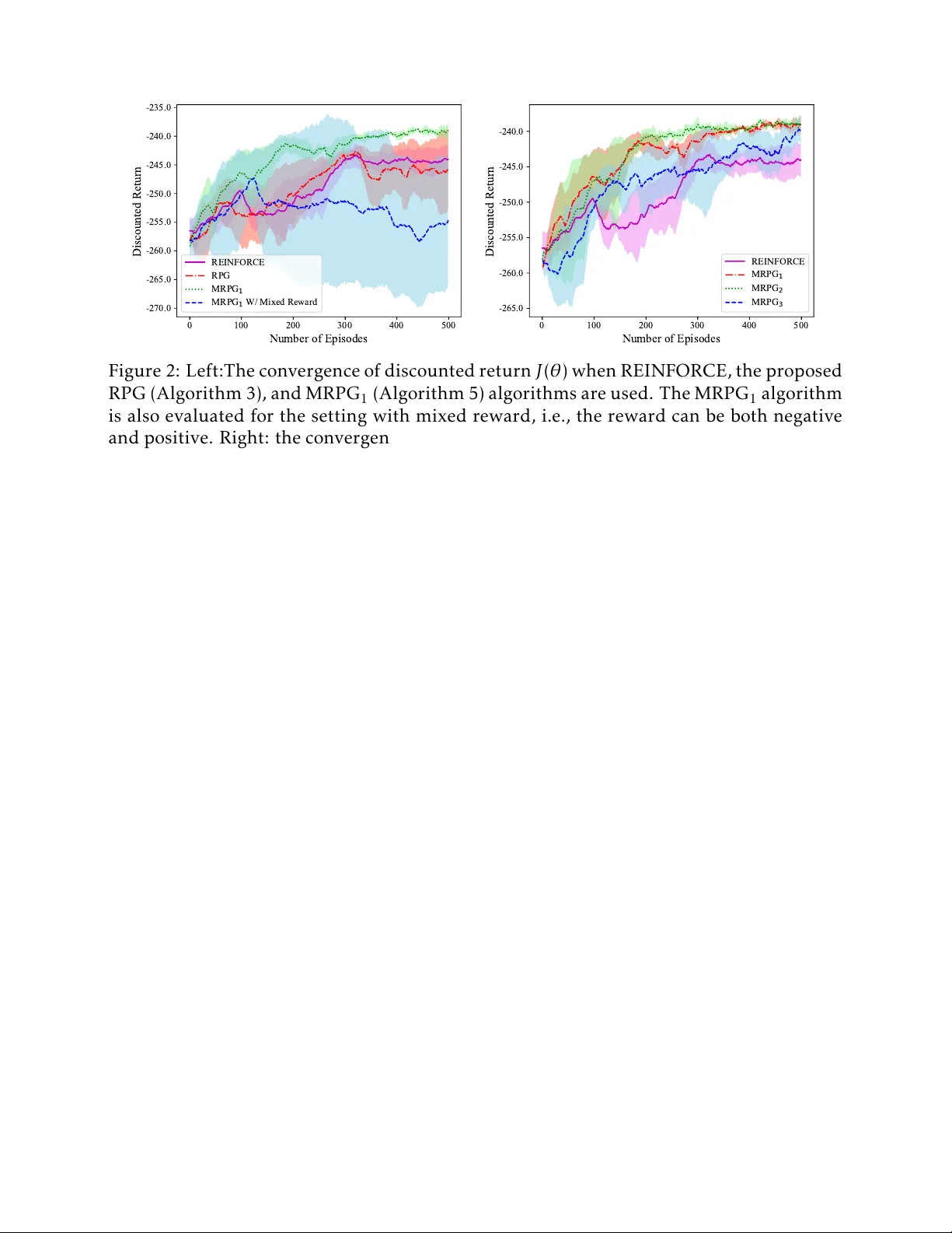
Global Con v ergence of P olicy Gradient Methods to (Almost) Locally Optimal P olicies Kaiqing Zhang Alec K oppel Hao Zhu T amer Bas ¸ ar J an uary 3, 2019 Abstract P olicy gradient (PG) methods are a widely used reinforcement learning methodol- ogy in many applications such as videogames, autonomous driving, and robotics. In spite of its empirical success, a rigorous understanding of the global converg ence of PG methods is lacking in the literature. In this work, we close the gap by viewing PG methods from a nonconvex optimization perspective. In particular , we propose a new varian t of PG methods for inﬁnite-horizon problems that uses a random rollout hori- zon for the Monte-Car lo estimation of the policy gradient. This method then yields an unbiased estimate of the policy gradient with bounded variance, which enables the tools from nonconv ex optimization to be applied to establish global conv ergence. Employing this perspective, we ﬁrst recover the conv ergence results with rates to the stationary -point policies in the literature. More interestingly , motivated by advances in nonconv ex optimization, we modify the proposed PG method by introducing peri- odically enlarged stepsizes. The modiﬁed algorithm is shown to escape saddle points under mild assumptions on the reward and the policy parameterization. Under a fur - ther strict saddle points assumption, this result establishes conv ergence to essentially locally -optimal policies of the underl ying problem, and thus bridges the gap in ex- isting literature on the conv ergence of PG methods. Results from experiments on the inv erted pendul um are then provided to corroborate our theory , namely , by slightly re- shaping the reward function to satisfy our assumption, unfa vorable saddle points can be av oided and better limit points can be attained. Intriguingly , this empirical ﬁnding justiﬁes the beneﬁt of reward-reshaping from a nonconv ex optimization perspective. 1 Introd uction In reinforcement learning (RL) [1, 2], an a utonomous agen t mov es through a state space and seeks to learn a policy which maps states to a probability distribution over actions to maximize a long-term accumulation of rewards. When the agent selects a given action at a particular state, a reward is rev ealed and a random transition to a new state occurs according to a probability density that only depends on the current state and action, i.e., state transitions are Markovian. This evol ution process is usually modeled as a Markov decision process (MDP). Under this setting, the ag ent m ust ev aluate the merit of di ﬀ erent 1 actions by interacting with the environmen t. T wo dominant approaches to reinforcement learning have emerg ed: those based on optimizing the accumulated reward directly from the policy space, referred to as “direct policy search ” , and those based on ﬁnding the val ue function by solving the Bellman ﬁxed point equations [3]. The goal of this wor k is to rig orously understand the former approach of direct policy search, speciﬁcally policy gradient (PG) methods [4]. P olicy search has gained traction recently , thanks to its ability to scale gracefull y to large and even contin uous spaces [5, 6] and to incorporate deep networ ks as function approximators [7, 8]. Despite the increasing prevalence of policy gradient methods, their global converg ence in the inﬁnite-horizon discounted setting, which is conventional in dynamic programming [2], is not yet well understood. This gap stems ﬁrstly from the f act that obtaining unbiased estimates of the policy gradient through sampling is often elusiv e. Speciﬁcally , foll owing the P olicy Gradient Theorem [4], obtaining an unbiased estimate of the policy gradient requires two signiﬁcant conditions to hold: (i) the state- action pair is drawn from the discounted state- action occupancy measure of the Markov chain under the policy; (ii) the estimate of the action-val ue (or Q ) function induced by the policy is unbiased. This gap also results from the f act that the value function to be maximized in RL is in general nonconvex with respect to the policy parameter [9, 10, 11, 12, 13]. In the same vein as our wor k, there is a surging interest in studying the global conv ergence of PG methods, see the recent work [9, 10, 14], and concurrent work [11, 12, 13]. In particular , orthogonal to our wor k, these work considered converg ence to the global optimum in several special RL settings: [9, 10, 14] considered the linear quadratic setting, [11, 13] considered the tabular setting, [12, 15] focused on the setting with overpar ameterized neural networks for function approximation, and [13] also considered the setting when the optimality gap of using certain policy class can be quantiﬁed. In contrast , our focus is on the case where the nonconv exity might be general, so that sol ving the problem can be NP -hard. When one restricts the focus to episodic reinforcement learning, Monte-Car lo rollout ma y be used to obtain unbiased estimates of the Q-function. In particular , the rollout simula tes the MDP under certain policy up to a ﬁnite time horizon, and then collects the rewards and state-action histories along the trajectory . Howev er , this ﬁnite-horizon rollout , though generally used in practice, is known to introduce bias in estimating an inﬁnite-horizon discounted v alue function. Such a bias in estimating the policy gradient for inﬁnite-horizon problems has been identiﬁed in the ear lier work [16, 17], both an- alytically and empirically . T o address this bias issue, we employ in this wor k random geometric time rollout horizons, a technique ﬁrst proposed in [18]. This rollout proce- dure allows us to obtain unbiased estimates of the Q function, using only rollouts of ﬁnite horizons. Moreover , the random rollout horizon also creates an unbiased sampling of the state- action pair from the discounted occupancy measure [4]. With these two challenges addressed, the policy gradien t can be estimated unbiasedly . Consequentl y , the policy gra- dient methods can be more naturally connected to the classical stochastic programming algorithms [19], where the unbiasedness of the stochastic gradient is a critical assumption. W e refer to our algorithm as random-horizon policy gradient (RPG), to emphasize that the ﬁnite horizon of the Monte-Car lo rollout is random. Lever aging this connection, we are able to address a noticeably open issue in policy gra- dient methods: a technical understanding of the e ﬀ ect of the policy parameterization on 2 both the limiting and ﬁnite-iteration algorithm behaviors. In particular , it is well known in nonconv ex optimization that with only ﬁrst -order information and no additional hy - pothesis, converg ence to a stationary point with zero gradient -norm is the best one may hope to achieve [20]. Indeed, this is the type of points that most current PG methods are guaranteed to converg e to, as pointed out by [13]. Howev er , in some asymptotic analy- ses for policy gradient methods with function approximation [21], or their variant , actor - critic algorithms [22, 23, 24, 25], it was claimed that the limit points of the algorithms starting from any initialization constitute the locally-optimal policies , i.e., the algorithms enjoy global conv ergence to the local-optima. How ever , by the theory of stochastic ap- proximation [26], such a claim can onl y be made locally , i.e., the local-optimality can only be obtained if the algorithm starts around a local minima, under the assumption that a strict L yapunov function exists. Therefore, global conv ergence of PG methods to the ac- tual locally-optimal policies, though claimed in words in some literature, is still an open question. Another line of theoretical studies of policy gradient methods only focuses on showing the one-step policy improv ement [27, 21, 28], by choosing appropriate stepsizes and/or batch data sizes. Such one-step result still does not imply any global converg ence result. In summary , the misuse of the term locally-optimal policy and the lack of study- ing global conv ergence property of PG methods motiv ate us to further inv estigate this problem from a nonconvex optimization perspective. Thanks to the analytical tools from optimization, we are able to ﬁrst recover the asymptotic conv ergence, and then provide the conv ergence rate, to stationary-point policies. Encouraged by this connection betw een noncon vex optimization and policy search, we then tackle a related question: what implications do recent algorithms that can escape saddle points for nonconv ex problems ([29, 30]) hav e on policy gradient methods in RL? T o answer this question, we identify several structural properties of RL problems tha t can be exploited to mitigate the underlying nonconvexity , which rely on some key assumptions on the policy parameterization and reward. Speciﬁcally , the reward needs to be bounded and either strictly positive or negativ e, and the policy parameterization need to be regular , i.e., its Fisher information matrix is positive deﬁnite (a conven tional assumption in RL [31]). Under these mild conditions, we can establish that policy gradient methods can escape saddle points and converg e to approximate second-order stationary points with high probability, when a periodically enlarged stepsize strategy is empl oyed. W e refer to the resulting method as Modiﬁed RPG (MRPG). Nevertheless, the strict positivity/nega tivity of reward function may amplify the variance of the gradient estimate, compared to the setting that has reward val ues with both signs but of smaller magnitude. This increased variance can be alleviated by introd ucing a baseline in the gradient estimate, as adv ocated by existing work [32, 33, 22]. Therefore, we propose two further modiﬁed updates that include the baselines, both shown to converg e to approximate second-order stationary points as w ell. Main Contribution: The main contribution of the present work is three-fold: i) we pro- pose a series of random-horizon PG methods that unbiasedly estimate the true policy gradient for inﬁnite-horizon discounted MDP s, which facilita tes the use of analytical tools from nonconv ex optimization to establish their conv ergence to stationary-point policies; ii) by virtue of such a connection of PG methods and nonconvex optimization, we pro- 3 pose modiﬁed RPG methods with periodically enlarged stepsizes, with guaranteed con- verg ence to actual locally-optimal policies under mil d conditions on the reward functions and parametrization of the policies; iii) we connect the condition on the reward function to the reward-reshaping technique advoca ted in empirical RL studies, justifying its beneﬁt, both analytically and empirically , from a nonconv ex optimization perspective. Addition- ally , we believe such a perspective opens the door to exploiting more advancemen ts in nonconv ex optimization to improve the converg ence properties of policy gradient meth- ods in RL. The rest of the paper is organized as follows. In §2, we clarify the problem setting of reinforcement learning and the technicalities of Markov Decision Processes. In §3 we devel op the policy gradient method using random geometric Monte-Carl o rollout hori- zons, i.e., the RPG method. Further , w e establish both its limiting (Theorem 4.2) and ﬁnite-sample (Theorem 4.3 and Corollary 4.4) behaviors under standard conditions. W e note tha t Corollary 4.4 provides one of the ﬁrst constant learning rate results in reinforce- ment learning. In §5, w e focus on problems with positive bounded rewards and policies whose parameterizations are regular , and propose a v ariant of policy gr adient method that empl oys a periodically enlarged stepsize scheme. The salient feature of this modiﬁed algo- rithm is that it is able to escape saddle points, an undesirable subset of stationary points, and conv erge to approximate second-order stationary points (Theorem 5.6). Numerical experiments in §6 corroborate our main ﬁndings: for Alg orithm 3, the use of random roll- out horizons avoids stochastic gradient bias and hence exhibits reliable converg ence that matches the theoretically established rates; moreov er , for the modiﬁed RPG algorithm, use of periodically enlarged stepsizes makes it possible to escape from undesir able saddle points and yields better limiting solutions. All proofs, which constitute an integral part of the paper , are relegated to nine appendices at the end of the paper , so as not to disrupt the ﬂow of the presenta tion of the main results. Notations: W e denote the probability distribution ov er the space S by P ( S ), and the set of integers { 1 , · · · , N } by [ N ]. W e use R to denote the set of real n umbers, and E to denote the expectation opera tor . W e let k · k denote the 2-norm of a vector in R d , or the spectr al norm of a matrix in R d × d . W e use |A| to denote the cardinality of a ﬁnite set A , or the area of a region A , i.e., |A| = R A d a . For an y matrix A ∈ R d × d , we use A  0 and A  0 to denote that A is positive deﬁnite and positiv e semi-deﬁnite, respectivel y . W e use λ min ( A ) and λ max ( A ) to denote, respectively , the smallest and largest eigenv alues of some square symmetric matrix A , respectiv ely . W e use E X or E X ∼ f ( x ) to denote the expectation with respect to random variable X . Otherwise speciﬁed, we use E to denote the full expectation with respect to all random v ariables. 2 Problem Form ulation In reinforcement learning, an autonomous ag ent moves through a state space S and takes actions that belong to some action space A . Here the spaces S and A are allowed to be either ﬁnite sets, or compact real v ector spaces, i.e., S ⊆ R q and A ⊆ R p . An action at the state causes a transition to the next state, where the transition mapping that depends on the current state and action; every such transition generates a reward revealed by the en- 4 vironment. The goal is for the ag ent to accum ulate as much reward as possible in the long term. This situation can be formalized as a Markov decision process (MDP) characterized by a tuple ( S , A , P , R, γ ) with Markov kernel P ( s 0 | s , a ) : S × A → P ( S ) that determines the transition probability from ( s , a ) to state s 0 . γ ∈ (0 , 1) is the discount factor . R ( · , · ) is the reward that is a function 1 of s and a . A t each time t , the agent executes an action a t ∈ A given the current state s t ∈ S , foll ow- ing a possibly stochastic policy π : S → P ( A ), i.e., a t ∼ π ( · | s t ). Then, giv en the state- action pair ( s t , a t ), the agent observes a reward r t = R ( s t , a t ). Thus, under an y policy π that maps states to actions, one can deﬁne the v alue function V π : S → R as V π ( s ) = E a t ∼ π ( · | s t ) ,s t +1 ∼ P ( · | s t ,a t ) ∞ X t =0 γ t r t      s 0 = s ! , which quantiﬁes the long term expected accumulation of rewards discounted by γ . W e can further deﬁne the val ue V π : S × A → R conditioned on a giv en initial action as the action- val ue, or Q-function as Q π ( s, a ) = E  P ∞ t =0 γ t r t    s 0 = s , a 0 = a  . W e also deﬁne A π ( s, a ) = Q π ( s, a ) − V π ( s ) for any s , a to be the advantage function . Given any initial state s 0 , the goal is to ﬁnd the optimal policy π that maximizes the long-term return V π ( s 0 ), i.e., to solv e the following optimiza tion problem max π ∈ Π V π ( s 0 ) , (2.1) when the model, i.e., the transition probability P and the reward function R , is unknown to the agent. In this work, we inv estigate policy search methods to solve (2.1). In general, we m ust search over an arbitrarily com plicated function class Π which may incl ude those which are unbounded and discontin uous. T o mitigate this issue, w e propose to par ameter - ize policies π in Π by a v ector θ ∈ R d , i.e., π = π θ , which giv es rise to RL alg orithms called policy gr adient methods [34, 23, 35]. With this parameterization, w e ma y reduce a search over arbitrarily complicated function class Π in (2.1) to one ov er the E uclidean space R d . Nonparametric parameterizations are also possible [ ? , ? ], but here we ﬁx the parameteriza- tion in order to sim plify exposition. For notational con venience, w e deﬁne J ( θ ) := V π θ ( s 0 ), then the vector -val ued optimization problem can be written as max θ ∈ R d J ( θ ) . (2.2) Generally , the value function is nonconv ex with respect to the parameter θ , meaning that obtaining a globally optimal solution to (2.2) is NP -hard, unless in several special RL settings that have been identiﬁed very recently [9, 11]. In fact, the limit point of most gradient -based methods to nonconvex optimization is a stationary solution, which could either be a saddle point or a local optimum. Usually the local optima achiev e reasonably good performance, in some cases comparable to the global optima, whereas the saddle points are undesirable and can stall training procedures. Therefore, it is beneﬁcial to design methods that ma y escape saddle points – see recent e ﬀ orts on escaping saddle 1 R ( s t , a t ) may be a random variable given ( s t , a t ). Here without loss of generality , we assume that it is deterministic for simplicity . 5 points with ﬁrst -order methods, e.g., perturbed gradient descent [36, 29, 30], and second- order methods [37, 38]. Our goal in this work is to develop stochastic gradient methods to maximize J ( θ ) and rigorously understand the interpla y between its limiting properties and the necessity of augmen ting the algorithmic update, reward function, and policy parameterization, all toward escaping undesirable limit points. This issue was ﬁrst observed and addressed in [39] by adding random perturbations in the reinforcement learning update (which may amplify v ariance), based on the asymptotic converg ence resul ts in [40]. Here we provide a modern perspective and incorpor ate the latest devel opments in nonconv ex optimization. 3 P olicy Gradient Methods In this section, we connect stochastic gradient ascent, as it is called in stochastic optimiza- tion, with the policy gradient method, a ﬂavor of direct policy search, in reinforcement learning. W e start with the following standard assumption on the regularity of the MDP problem and the smoothness of the parameterized policy π θ . Assumption 3.1. Suppose the reward function R and the parameterized policy π θ satisfy the following conditions: (i) The absolute val ue of the reward R is uniforml y bounded, sa y by U R , i.e., | R ( s, a ) | ∈ [0 , U R ] for an y ( s , a ) ∈ S × A . (ii) The policy π θ is di ﬀ erentiable with respect to θ , and ∇ log π θ ( a | s ), known as the score function corresponding to the distribution π θ ( · | s ), exists. Moreover , it is L Θ -Lipschitz and has bounded norm for an y ( s , a ) ∈ S × A , k∇ log π θ 1 ( a | s ) − ∇ log π θ 2 ( a | s ) k ≤ L Θ · k θ 1 − θ 2 k , for an y θ 1 , θ 2 , (3.1) k∇ log π θ ( a | s ) k ≤ B Θ , for some constant B Θ for an y θ . (3.2) for some constant B Θ > 0. Note that the boundedness of the reward function in Assumption3.1(i) is standard in the literature of policy gradient/actor -critic alg orithms [22, 23, 35, 41, 42]. The uniform boundedness of R also implies that the absolute v alue of the Q-function is upper bounded by U R / (1 − γ ), since by deﬁnition | Q π θ ( s, a ) | ≤ ∞ X t =0 γ t · U R = U R / (1 − γ ) , for an y ( s, a ) ∈ S × A . The same bound also applies to V π θ ( s ) for an y π θ and s ∈ S , and thus to the objective J ( θ ) which is deﬁned as V π θ ( s 0 ), i.e., | V π θ ( s ) | ≤ U R / (1 − γ ) , for an y s ∈ S , | J ( θ ) | ≤ U R / (1 − γ ) . In addition, the conditions (3.1) and (3.2) have also been adopted in several recent wor k on the con verg ence analysis of policy gradient algorithms [35, 21, 43, 44]. Both of 6 the conditions can be readil y sa tisﬁed by man y common parametrized policies such as the Boltzmann policy [39] and the Gaussian policy [45]. For example, for Gaussian policy 2 in contin uous spaces, π θ ( · | s ) = N ( φ ( s ) > θ , σ 2 ), where N ( µ, σ 2 ) denotes the Gaussian dis- tribution with mean µ and variance σ 2 , and φ ( s ) is the feature vector that incorporates some domain knowledge to approximate the mean action at state s . Then the score func- tion has the form [ a − φ ( s ) > θ ] φ ( s ) / σ 2 , which satisﬁes (3.1) and (3.2) if the foll owing three conditions hold: the norm of the f eature k φ ( s ) k is bounded; the parameter θ lies in some bounded set; and the actions a ∈ A is bounded. Under Assumption 3.1, the gradient of J ( θ ) with respect to the policy parameter θ , given by the P olicy Gradient Theorem [4], has the following f orm 3 : ∇ J ( θ ) = Z s ∈S ,a ∈A ∞ X t =0 γ t · p ( s t = s | s 0 , π θ ) · ∇ π θ ( a | s ) · Q π θ ( s, a ) d sd a (3.3) = 1 1 − γ Z s ∈S ,a ∈A (1 − γ ) ∞ X t =0 γ t · p ( s t = s | s 0 , π θ ) · ∇ π θ ( a | s ) · Q π θ ( s, a ) d sd a = 1 1 − γ Z s ∈S ,a ∈A ρ π θ ( s ) · π θ ( a | s ) · ∇ log[ π θ ( a | s )] · Q π θ ( s, a ) d sd a = 1 1 − γ · E ( s,a ) ∼ ρ θ ( · , · ) h ∇ log π θ ( a | s ) · Q π θ ( s, a ) i . (3.4) Here, we denote by p ( s t = s | s 0 , π θ ) the probability that state s t equals s given initial state s 0 and policy parameter θ , and the distribution ρ π θ ( s ) = (1 − γ ) P ∞ t =0 γ t p ( s t = s | s 0 , π θ ) which has been shown to be a valid probability measure over the state S in [4]. W e refer to ρ π θ ( s ) as the discounted state-occupancy measure hereafter . For notational conv enience, we let ρ θ ( s, a ) = ρ π θ ( s ) · π θ ( a | s ), which denotes the discounted state-action occupancy measure . In addition, based on the fact that f or any function b : S → R independent of action a , Z a ∈A π θ ( a | s ) ∇ log π θ ( a | s ) · b ( s ) d a = ∇ Z a ∈A π θ ( a | s ) d a · b ( s ) = ∇ 1 · b ( s ) = 0 , f or any s ∈ S , the policy gradient in (3.4) can be written as ∇ J ( θ ) = 1 1 − γ · E ( s,a ) ∼ ρ θ ( · , · ) n ∇ log π θ ( a | s ) · [ Q π θ ( s, a ) − b ( s )] o , where b ( s ) is usually referred to as a baseline function. One common choice of the base- line is the state-v alue function V π θ ( s ), which giv es the foll owing advantag e-based policy gradient ∇ J ( θ ) = 1 1 − γ · E ( s,a ) ∼ ρ θ ( · , · ) n ∇ log π θ ( a | s ) · A π θ ( s, a ) o . (3.5) 2 Note that in practice, the action space A is bounded, thus a truncated Gaussian policy over A is often used; see [43]. 3 Note that here we use R to represent both summation over ﬁnite sets and integral over continuous spaces. 7 Algorithm 1 EstQ: Unbiasedly Estimating Q-function Input: s , a , and θ . Initialize ˆ Q ← 0, s 0 ← s , and a 0 ← a . Draw T from the geometric distribution Geom(1 − γ 1 / 2 ), i.e., P ( T = t ) = (1 − γ 1 / 2 ) γ t / 2 . for all t = 0 , · · · , T − 1 do Collect and add the instantaneous reward R ( s t , a t ) to ˆ Q , ˆ Q ← ˆ Q + γ t / 2 · R ( s t , a t ). Simula te the next state s t +1 ∼ P ( · | s t , a t ) and action a t +1 ∼ π ( · | s t +1 ). end for Collect R ( s T , a T ) by ˆ Q ← ˆ Q + γ T / 2 · R ( s T , a T ). return ˆ Q . In this wor k, w e devise methods that can use iterativ e updates based on the classical pol- icy gradient (3.4) or its variant that makes use of the advantage function (3.5) through the aforementioned identity regarding baselines. First note that under Assumption 3.1, we can establish the Lipschitz continuity of the policy gradient ∇ J ( θ ) as in the foll owing lemma, whose proof is deferred to §A.1. Lemma 3.2 (Lipschitz-Contin uity of P olicy Gradient) . Under Assumption 3.1, the policy gradient ∇ J ( θ ) is Lipschitz continuous with some constant L > 0, i.e., for an y θ 1 , θ 2 ∈ R d k∇ J ( θ 1 ) − ∇ J ( θ 2 ) k ≤ L · k θ 1 − θ 2 k , where the val ue of the Lipschitz constant L is deﬁned as L := U R · L Θ (1 − γ ) 2 + (1 + γ ) · U R · B 2 Θ (1 − γ ) 3 . (3.6) Next, we discuss how (3.4) and (3.5) can be used to devel op ﬁrst -order stochastic ap- proximation methods to address (2.2). Unbiased samples of the gradient ∇ J ( θ ) are re- quired to perform the stochastic gradient ascent, which hopefully conv erges to a station- ary sol ution of the nonconv ex optimization problem. Moreover , through the addition of carefully designed perturbations, we aim to attain a local optimum, namely , asymptoti- cally stable stationary point , as in [39, 36, 29]. Sampling the P olicy Gradient: In order to obtain an unbiased sample of ∇ J ( θ ), it is nec- essary to: i) draw state-action pair ( s , a ) from the distribution ρ θ ( · , · ); and ii) obtain an un- biased estimate of the Q-function Q π θ ( s, a ), or the advantag e function A π θ ( s, a ) eval uated at ( s, a ). Both of the requirements can be satisﬁed by using a random horizon T that follows cer - tain geometric distribution in the sam pling process. In particular , to ensure the condition i) is satisﬁed, we use the last sample ( s T , a T ) of a ﬁnite sample trajectory ( s 0 , a 0 , s 1 , · · · , s T , a T ) to be the sample at which Q π θ ( · , · ) and ∇ log π θ ( · | · ) are eval uated, where the horizon T ∼ Geom(1 − γ ). It can be shown that ( s T , a T ) ∼ ρ θ ( · , · ). Moreover , given ( s T , a T ), we perform Monte-Car lo rollouts for another horizon T 0 ∼ Geom(1 − γ 1 / 2 ) independent of T , and es- timate the Q-function v alue Q π θ ( s, a ) as f ollows by collecting the γ 1 / 2 -discounted rewards 8 Algorithm 2 EstV : Unbiasedly Estimating S tate- V alue function Input: s and θ . Initialize ˆ V ← 0, s 0 ← s , and draw a 0 ∼ π θ ( · | s 0 ). Draw T from the geometric distribution Geom(1 − γ 1 / 2 ). for all t = 0 , · · · , T − 1 do Collect the instantaneous reward R ( s t , a t ) and add to val ue ˆ V ; ˆ V ← ˆ V + γ t / 2 · R ( s t , a t ). Simula te the next state s t +1 ∼ P ( · | s t , a t ) and action a t +1 ∼ π ( · | s t +1 ). end for Collect R ( s T , a T ) by ˆ V ← ˆ V + γ T / 2 · R ( s T , a T ). return ˆ V . along the trajectory: ˆ Q π θ ( s, a ) = T 0 X t =0 γ t / 2 · R ( s t , a t )    s 0 = s , a 0 = a. (3.7) Then, it can be shown that ˆ Q π θ ( s, a ) unbiasedly estimates Q π θ ( s, a ) for any ( s , a ) (see The- orem 3.4, whose proof is given in Appendix A.2). The subroutine of estimating the Q- function is summarized as EstQ in Algorithm 1. Remark 3.3. Thanks to randomness of the horizon, we note that the aforementioned sampling process creates the ﬁrst unbiased estimate of the Q-function in the discounted inﬁnite-horizon setting, using the Monte-Car lo rollouts of ﬁnite horizons . While in pr actice, usually ﬁnite-horizon rollouts are used to approximate the inﬁnite-horizon Q-function, e.g., in the REINFORCE algorithm, which causes bias in the Q-function estimate, and hence the policy gr adient estimate. Our sampling technique addresses this challenge, and ends up with an unbiased estimate of the policy gradient as to be introduced next. W e note that the proposed sampling technique for estimating the Q-function improves the one in [18] that uses Geom(1 − γ ) (instead of Geom(1 − γ 1 / 2 )) to generate the rollout hori- zon T 0 . In particular , the proposed Q-function estimate is almost surely bounded thanks to the γ 1 / 2 -discount factor in (3.7), which later leads to almost sure boundedness of the stochastic policy gr adient, a necessary assumption required in the con verg ence analysis to approximate second-order stationary points in §5. Motiva ted by the form of policy gradient in (3.4), we propose the foll owing stochastic estimate ˆ ∇ J ( θ ) ˆ ∇ J ( θ ) = 1 1 − γ · ˆ Q π θ ( s T , a T ) · ∇ log[ π θ ( a T | s T )] . (3.8) In addition, we can also estimate the policy gradient using adv antage functions as in (3.5), where the advantag e function is estimated by either the di ﬀ erence between the value func- tion and the action-v alue function, or the temporal di ﬀ erence (TD) error . In particular , we propose the following tw o stochastic policy gradients ˇ ∇ J ( θ ) = 1 1 − γ · [ ˆ Q π θ ( s T , a T ) − ˆ V π θ ( s T )] · ∇ log[ π θ ( a T | s T )] , (3.9) e ∇ J ( θ ) = 1 1 − γ · [ R ( s T , a T ) + γ ˆ V π θ ( s 0 T ) − ˆ V π θ ( s T )] · ∇ log[ π θ ( a T | s T )] , (3.10) 9 where ˆ V π θ ( s ) is an unbiased estimate of the v alue function V π θ ( s ), and s 0 T is the next state given state s T and a T . The process of estimating ˆ V π θ ( s ) employs the same idea as the EstQ algorithm, where ˆ V π θ ( s ) is obtained by collecting the γ 1 / 2 -discounted rewards along the trajectory starting from s 0 (instead of a state- action pair ( s , a )), following a t ∼ π θ ( · | s t ), and of length T 0 ∼ Geom(1 − γ 1 / 2 ), i.e., ˆ V π θ ( s ) = P T 0 t =0 γ 1 / 2 · R ( s t , a t ) | s 0 = s . W e refer to this subroutine as EstV , which is summarized in Algorithm 2. The reason for these al ternate updates is that the o ﬀ -set term can be used to reduce the v ariance of estimating the policy gradient [32]. W e then establish in the following theorem, which states that all the stochastic policy gradients ˆ ∇ J ( θ ) , ˇ ∇ J ( θ ), and e ∇ J ( θ ) are unbiased estimates of ∇ J ( θ ) [cf. (3.4)]. Additionally , we can also establish the boundedness of k ˆ ∇ J ( θ ) k , k ˇ ∇ J ( θ ) k , and k e ∇ J ( θ ) k , as well as k∇ J ( θ ) k for an y θ ∈ Θ . The proof is deferred to Appendix A.2. Theorem 3.4 (Properties of Stochastic P olicy Gradients) . For any θ , ˆ ∇ J ( θ ) , ˇ ∇ J ( θ ), and e ∇ J ( θ ) obtained from (3.8), (3.9), and (3.10), respectiv ely , are all unbiased estimates of ∇ J ( θ ) in (3.4), i.e., for an y θ E [ ˆ ∇ J ( θ ) | θ ] = E [ ˇ ∇ J ( θ ) | θ ] = E [ e ∇ J ( θ ) | θ ] = ∇ J ( θ ) . where the expectation is with respect to the random horizon T 0 , the trajectory along ( s 0 , a 0 , s 1 , · · · , s T 0 , a T 0 ), and the random sample ( s T , a T ). Moreover , the norm of the policy gradient ∇ J ( θ ) is bounded, and its stochastic estimates ˆ ∇ J ( θ ) , ˇ ∇ J ( θ ) , e ∇ J ( θ ) are all almost surely (a.s.) bounded, i.e., k∇ J ( θ ) k ≤ B Θ · U R (1 − γ ) 2 , k ˆ ∇ J ( θ ) k ≤ ˆ ` a.s. , k ˇ ∇ J ( θ ) k ≤ ˇ ` a.s. , k e ∇ J ( θ ) k ≤ e ` a.s. , for some constants ˆ ` , ˇ ` , e ` > 0, whose values are giv en in (A.19), (A.20), and (A.21) in §A.2. Henceforth in this section and the next , w e will mainly f ocus on the conv ergence anal- ysis f or the RPG algorithm with the stochastic gradient ˆ ∇ J ( θ ) as deﬁned in (3.8). The RPG algorithms with ˇ ∇ J ( θ ) and e ∇ J ( θ ) will be discussed later in §5, where red ucing the variance of RPG is of greater interest. T o this end, let k be the iteration index and θ k be the associa ted estimate for the policy parameter . Under Theorem 3.4, the policy gradient update f or step k + 1 is θ k +1 = θ k + α k ˆ ∇ J ( θ k ) = θ k + α k 1 − γ · ˆ Q π θ k ( s T k +1 , a T k +1 ) · ∇ log[ π θ k ( a T k +1 | s T k +1 )] , (3.11) where { α k } is the stepsize sequence that can be either diminishing or constant, and { T k } are drawn i.i.d. from Geom(1 − γ ). The details of the policy gradient method, which we ref er to as the random-horizon policy gradient algorithm, are summarized in Algorithm 3. Note that the estima te of ˆ Q π θ k ( s T k +1 , a T k +1 ), i.e., Alg orithm 1, is conducted in the inner -loop of the stochastic policy gradient update. Remark 3.5. W e note that in order to estimate the Q-function, it is not very sample- e ﬃ cient to use Monte-Car lo rollouts to sample states, actions, and rewards. In fact , there 10 Algorithm 3 RPG: Random-horizon P olicy Gradient Al gorithm Input: s 0 and θ 0 , initialize k ← 0. Repeat: Draw T k +1 from the geometric distribution Geom(1 − γ ). Draw a 0 ∼ π θ k ( · | s 0 ) for all t = 0 , · · · , T k +1 − 1 do Simula te the next state s t +1 ∼ P ( · | s t , a t ) and action a t +1 ∼ π θ k ( · | s t +1 ). end for Obtain an estimate of Q π θ k ( s T k +1 , a T k +1 ) by Algorithm 1, i.e., ˆ Q π θ k ( s T k +1 , a T k +1 ) ← EstQ ( s T k +1 , a T k +1 , θ k ) . P erform policy gradient upda te θ k +1 ← θ k + α k 1 − γ · ˆ Q π θ k ( s T k +1 , a T k +1 ) · ∇ log[ π θ k ( a T k +1 | s T k +1 )] Update the itera tion counter k ← k + 1. Until Conv ergence exist some methods that can estimate the Q-function in parallel with the policy gradient update, which is usually referred to as actor -critic method [34, 23]. This online policy eval uation update is generally performed via bootstrapping algorithms such as temporal di ﬀ erence learning [46], which will introduce biases into the Q-function estimate, and thus the policy gradient estimate. In addition, such policy evalua tion updates in concur - rence with the policy improv ement will inevitably cause correlation between consecutive stochastic policy gradients. Analyzing the non- asymptotic converg ence performance of such biased RPG with corr elated noise is still open and challenging, which is left as a future research direction. In the next sections, we shift focus to anal yzing the theoretical properties of the afore- mentioned policy learning methods, establishing their asymptotic and ﬁnite-time perfor - mances, as well as stepsize strategies designed to mitigate the challenges of non-conv exity when certain reward structure is present. 4 Con verg ence to Sta tionary P oints In this section, we provide converg ence analyses for the policy gradient alg orithms pro- posed in §3. W e start with the following assumption for the diminishing stepsize α k , which is standard in stochastic approximation. 11 Assumption 4.1. The sequence of stepsize { α k } k ≥ 0 satisﬁes the Robbins-Monro condition ∞ X k =0 α k = ∞ , ∞ X k =0 α 2 k < ∞ . W e ﬁrst establish the conv ergence of Alg orithm 3 in the following theorem under the aforementioned technical conditions. Theorem 4.2 (Asymptotic Converg ence of Algorithm 3) . Let { θ k } k ≥ 0 be the sequence of parameters of the policy π θ k given by Alg orithm 3. Then under Assumptions 3.1 and 4.1, we ha ve lim k →∞ θ k ∈ Θ ∗ , where Θ ∗ is the set of stationary points of J ( θ ). Theorem 4.2, whose proof is in Appendix A.3, shows that the random-horizon policy gradient update conv erges to the (ﬁrst -order) stationary points of J ( θ ) almost surely . The proof of the theorem is relegated to §A.3. W e note that the asymptotic converg ence result here is established from an optimization perspectiv e using supermartingale converg ence theorem [47], which di ﬀ ers from the existing techniques that show converg ence of actor - critic algorithms from dynamical systems theory (or ODE method) [26]. Such optimization perspective can be lev eraged thanks to the unbiasedness of the stochastic policy gradients obtained from Algorithm 3. An additional virtue of this style of analysis is that we can also establish con verg ence rate of the policy gradient al gorithm without the need for sophisticated concentration inequalities. In contrast, the ﬁnite-iteration analysis for actor -critic algorithms is known to be quite challenging [48, 49]. By conv ention, we choose the stepsize to be either α k = k − a for some parameter a ∈ (0 , 1) or constant α > 0. Note that for the diminishing stepsize, here we allow a more general choice than that in Assumption 4.1. Since J ( θ ) is generall y nonconv ex, we consider the converg ence rate in terms of a metric of nonstationarity , i.e., the norm of the gradient k∇ J ( θ k ) k . W e then provide the converg ence rates of Algorithm 3 for the setting of using diminishing and constant stepsizes in the f ollowing theorem and corollary , respectively . The proofs of the results are giv en in §A.4. Theorem 4.3 (Conv ergence Rate of Algorithm 3 with Diminishing Stepsize) . Let { θ k } k ≥ 0 be the sequence of parameters of the policy π θ k given by Algorithm 3. Let the stepsize be α k = k − a where a ∈ (0 , 1). Let K  = min n k : inf 0 ≤ m ≤ k E k∇ J ( θ m ) k 2 ≤  o . Then, under Assumption 3.1, w e hav e K  ≤ O (  − 1 / p ), where p is deﬁned as p = min { 1 − a, a } . By optimizing the complexity bound ov er a , we obtain K  ≤ O (  − 2 ) with a = 1 / 2. Corollary 4.4 (Converg ence Rate of Algorithm 3 with Constant S tepsize) . Let { θ k } k ≥ 0 be the sequence of parameters of the policy π θ k given by Algorithm 3. Let the stepsize be α k = α > 0. Then, under Assumption 3.1, w e have 1 k k X m =1 E k∇ J ( θ m ) k 2 ≤ O ( α L ˆ ` 2 ) , where recall that L is the Lipchitz constant of the policy gradient as deﬁned in (3.6) in Lemma 3.2. 12 Theorem 4.3 illustr ates that when diminishing stepsize is adopted, which essentially establishes a 1 / √ k conv ergence rate for the conv ergence of the expected gradient norm square k∇ J ( θ k ) k 2 . Corollary 4.4 shows that the aver age of the gradient norm square will conv erge to a neighborhood around zero with the rate of 1 / k . The size of the neighbor - hood is controlled by the stepsize α . Moreover , (A.37) also implies that a smaller stepsize ma y decrease the size of the neighborhood, at the expense of the con vergence speed. W e note that both results are standard and recover the conv ergence properties of stochastic gradient descent for nonconv ex optimization problems [19, 50]. In the next section, we propose modiﬁed stepsize rules, which under an appropriate hypothesis on the policy parameterization and reward structure of the problem, yiel d stronger limiting policies. 5 Con verg ence to Second-Order Sta tionary P oints In this section, we provide converg ence analyses for several modiﬁed policy gradient al- gorithms based on Algorithm 3, which may escape saddle points and thus conv erge to the approximate second-order stationary points of the problem. In short, we propose a custom periodically enlarged stepsize rule, which under an additional h ypothesis on the incentiv e structure of the problem and some other standard conditions (see §5.1), allow us to attain improv ed limiting policy parameters (see §5.2). W e start with the deﬁnition of (approximate) second-order stationary points [51] 4 . Deﬁnition 5.1. An (  g ,  h )-approximate-second-order stationary point θ is deﬁned as k∇ J ( θ ) k ≤  g , λ max [ ∇ 2 J ( θ )] ≤  h . If  g =  h = 0, the point θ is a second-order stationary point. The in tuition for this deﬁnition is that a local maximum is one in which the gradient is null and the Hessian is negativ e semideﬁnite. When we relax the ﬁrst criterion, we obtain the ﬁrst inequality , whereas when we relax the second one, we mean that the Hessian is near negativ e semideﬁnite. With the further assumption that all saddle points are strict (i.e., for an y saddle point θ , λ max [ ∇ 2 J ( θ )] > 0) [29, 36], all second-order stationary poin ts (  g =  h = 0) are local max- ima. In this case, conv erging to (approximate) second-order stationary points is equivalent to conv erging to approximate local minima, which is usually more desirable than converg- ing to (ﬁrst -order) stationary points. 5.1 Alg orithm The modiﬁed RPG (MRPG) algorithms are built upon the RPG algorithm (Alg orithm 3) discussed in Section 3. These modiﬁcations can yield escape from saddle points under certain conditions, and hence conv ergence to approximate l ocal extrema. 4 Note that Deﬁnition 5.1 is based on the maximization problem we consider here, which is slightly dif - ferent from the deﬁnition f or minimization problems where λ max [ ∇ 2 J ( θ )] ≤  h is replaced by λ min [ ∇ 2 J ( θ )] ≥ −  h . 13 Algorithm 4 EvalPG: Calcula ting the Three T ypes of Stochastic P olicy Gradients Input: s , a , θ and the gradient type ♦ . if gradient type ♦ = ˆ then Obtain an estimate ˆ Q π θ ( s, a ) ← EstQ ( s , a, θ ). Calcula te ˆ ∇ J ( θ ), i.e., let g θ ← 1 1 − γ · ˆ Q π θ ( s, a ) · ∇ log π θ ( a | s ) . else if gradient type ♦ = ˇ then Obtain estimates ˆ Q π θ ( s, a ) ← EstQ ( s , a, θ ) and ˆ V π θ ( s ) ← EstV ( s , θ ). Calcula te ˇ ∇ J ( θ ), i.e., let g θ ← 1 1 − γ · [ ˆ Q π θ ( s, a ) − ˆ V π θ ( s )] · ∇ log π θ ( a | s ) . else if gradient type ♦ = e then Simula te the next state: s 0 ∼ P ( · | s , a ). Obtain estimates ˆ V π θ ( s ) ← EstV ( s , θ ) and ˆ V π θ ( s 0 ) ← EstV ( s 0 , θ ). Calcula te e ∇ J ( θ ), i.e., let g θ ← 1 1 − γ · [ R ( s , a ) + γ · ˆ V π θ ( s 0 ) − ˆ V π θ ( s )] · ∇ log π θ ( a | s ) . end if return Stochastic policy gradient g θ In order to reduce the variance of the RPG update (3.11), we empl oy the stochastic gradients ˇ ∇ J ( θ ) and e ∇ J ( θ ) as deﬁned in (3.9) and (3.10), respectively . Note that the eval- uations of both ˇ ∇ J ( θ ) and e ∇ J ( θ ) need to estimate the sta te-val ue function ˆ V π θ ( s ) for any given θ and s . Built upon the subroutines EstQ and EstV , w e summarize the subroutine for calcula ting all three types of stochastic policy gradients as EvalPG in Alg orithm 4. In order to conv erge to the approximate second-order stationary points, w e modify the RPG algorithm, i.e., Algorithm 3, by periodically enlarging the constant stepsize of the up- date, once every k thre steps. The larger stepsize can amplify the variance along the eigen- vector corresponding to the largest eigenv alue of the Hessian, which provides a direction for the update to escape at the saddle points. This idea w as ﬁrst introduced in [30] for gen- eral stochastic gradient methods, and is outlined in Alg orithm 5. Note that α and β are the constant stepsizes with β > α > 0, whose values will be given in §5.2 to obtain certain conv ergence rates. T o design this behavior while avoiding unnecessarily large variance, we propose updates that make use of the advantag e function, i.e., ˇ ∇ J ( θ ) and e ∇ J ( θ ). The resulting algorithm, with periodically enlarged stepsizes, and stochastic policy gradien ts that use advan tage functions, is summarized as Algorithm 5. Subsequently , w e shift focus to characterizing its policy learning performance anal ysis. 14 Algorithm 5 MRPG: Modiﬁed Random-horizon P olicy Gradient Al gorithm Input: s 0 , θ 0 , and the gradient type ♦ , initialize k ← 0, return set ˆ Θ ∗ ← ∅ . Repeat: Draw T k +1 from the geometric distribution Geom(1 − γ ), and dra w a 0 ∼ π θ k ( · | s 0 ). for all t = 0 , · · · , T k +1 − 1 do Simula te the next state s t +1 ∼ P ( · | s t , a t ) and action a t +1 ∼ π θ k ( · | s t +1 ). end for Calcula te the stochastic gradient g k ← EvalPG ( s T k +1 , a T k +1 , θ k , ♦ ). if ( k mod k thre ) = 0 then ˆ Θ ∗ ← ˆ Θ ∗ ∪ { θ k } θ k +1 ← θ k + β · g k else θ k +1 ← θ k + α · g k end if Update the itera tion counter k = k + 1. Until Conv ergence return θ uniformly at r andom from the set ˆ Θ ∗ . 5.2 Conv ergence Anal ysis In this subsection, we provide a ﬁnite-iteration conv ergence result for the modiﬁed RPG algorithm, i.e., Alg orithm 5. T o this end, we ﬁrst introduce the foll owing condition, built upon Assumption 3.1, which is required in the sequel. Assumption 5.2. The MDP and the parameterized policy π θ satisfy the following condi- tions: (i) The reward R ( s , a ) is either positive or negativ e for an y ( s , a ) ∈ S × A . Thus, | R ( s, a ) | ∈ [ L R , U R ] with some L R > 0. (ii) The score function ∇ log π θ exists, and its norm is bounded by k∇ l og π θ k ≤ B Θ for an y θ . Also, the J acobian of ∇ log π θ has bounded norm and is Lipschitz continuous, i.e., there exist constants ρ Θ > 0 and L Θ < ∞ such that for an y ( s , a ) ∈ S × A    ∇ 2 log π θ 1 ( a | s ) − ∇ 2 log π θ 2 ( a | s )    ≤ ρ Θ · k θ 1 − θ 2 k , for any θ 1 , θ 2 ,    ∇ 2 log π θ ( a | s )    ≤ L Θ , for any θ . (iii) The integral of the Fisher information matrix induced by π θ ( · | s ) is positiv e-deﬁnite 15 uniformly f or any θ ∈ R d , i.e., there exists a constant L I > 0 such that Z s ∈S ,a ∈A ρ θ ( s, a ) · ∇ log π θ ( · | s ) · [ ∇ log π θ ( · | s )] > d ad s  L I · I , for all θ ∈ R d . (5.1) W e note that Assumption 5.2 is indeed standard, and can be readily satisﬁed in prac- tice. First, the strict positivity (or negativity) of the reward function in Assumption 5.2(i) can be easily satisﬁed by adding (or subtracting) an o ﬀ set to the original non-negative and upper -bounded reward. In fact , it can be justiﬁed in the foll owing lemma that adding any o ﬀ set does not change the optimal policy of the original MDP . Lemma 5.3. Given an y MDP M = ( S , A , P , R, γ ), let f M be a modiﬁed MDP of M , such tha t M = ( S , A , P , e R, γ ) and e R ( s, a ) = R ( s, a ) + C , for any s ∈ S , a ∈ A , and C ∈ R . Then, the sets of optimal policies for the two MDP s, M and f M , are equal. The proof of the lemma is deferred to Appendix §A.5. The positivity (or negativity) of the rewards ensures that the absolute value of the Q-function is also l ower -bounded, by the v alue of L R / (1 − γ ), which will beneﬁt the conv ergence of the MRPG algorithm as to be speciﬁed shortly . Interestingly , such a reshape of the reward function can be shown to yield better conv ergence results. T o our knowledge, our w ork appears to be the ﬁrst theoretical study on the e ﬀ ect of reward-reshaping on the converg ence property of policy gradient methods, although reward-reshaping is known to be useful for improving learned policies in practice. On the other hand, we note that such positivity of | Q π θ | will cause a relativel y large variance in the original RPG update (3.11). This makes the RPG with baseline, i.e., the use of ˇ ∇ J ( θ ) and e ∇ J ( θ ), beneﬁcial for v ariance reduction. The latter conditions (ii)-(iii) in Assumption 5.2 can also be satisﬁed easily by com- monly used policies such as Gaussian policies and Gibbs policies. For example, for a Gaussian policy , ∇ 2 log π θ ( a | s ) reduces to the matrix φ ( s ) φ ( s ) > / σ 2 , which is a constant function of θ and thus satisﬁes condition (ii). Such a condition is used to show the Lip- schitz contin uity of the Hessian matrix of the objectiv e function J ( θ ) = V π θ ( s 0 ), which is standard in establishing the conv ergence to approximate second-order stationary points in the nonconv ex optimization literature [36, 29, 30, 38]. Formally , the Lipschitz conti- nuity of the Hessian is substantiated in the following lemma, whose proof is relegated to Appendix §A.6. Lemma 5.4. The Hessian matrix of the objective function H ( θ ) is Lipschitz continuous, i.e., with some constant ρ > 0,    H ( θ 1 ) − H ( θ 2 )    ≤ ρ · k θ 1 − θ 2 k , for any θ 1 , θ 2 ∈ R d . The val ue of the Lipschitz constant ρ is given in (A.68) in §A.6. The third condition (iii) in Assumption 5.2 holds for many regular policy parameteriza- tions, and has been assumed in prior w orks on na tural policy gradient [31] and actor -critic algorithms [23]. W e note that Assumption 5.2 implies Assumption 3.1. More speciﬁ- cally , the condition on the rew ard function in Assum ption 3.1 only requires boundedness, 16 P aram. V alue Order Constraint Equation Const. β c 1  2 / (2 ` 2 L ) O (  2 ) ≤  2 / (2 ` 2 L ) (A.90) c 1 = 1 β ” ” ≤ [ J thre δ/ (2 L` 2 )] 1 / 2 (A.92) ” β ” O (  ) ≤ η λ 2 / (24 L` 3 ρ ) (A.112) ” J thre c 2 η  4 / (2 ` 2 L ) O (  4 ) ≤ β  2 / 2 (A.91) c 2 = c 1 / 2 J thre ” ” ≤ η β λ 2 / (48 ` ρ ) (A.113) ” α c 1  2 / (2 ` 2 L √ k thre ) O (  9 / 2 ) ≤ β / √ k thre (A.89) α ” ” ≤ c 0 η β λ 3 / (24 L` 3 ρ ) (A.114) ” k thre c 4 log[ L` g / ( η β α √ ρ )] α ( ρ ) 1 / 2 Ω (  − 5 log(1 /  )) ≥ c log[ L` g / ( η β α λ )] α λ (A.115) c 4 = c K c 5 [ J ∗ − J ( θ 0 )] k thre δJ thre Ω (  − 9 log(1 /  )) ≥ 2 [ J ∗ − J ( θ 0 )] k thre δJ thre (A.96) c 5 = 2 T able 1: List of parameter v alues used in the con vergence anal ysis. without further requirement on its positivity/ negativity; the boundedness of the norm k∇ 2 log π θ ( a | s ) k in Assumption 5.2 implies the L Θ -Lipschitz continuity of the score func- tion ∇ log π θ ( a | s ) in Assumption 3.1. And the condition on the positiv e-deﬁniteness of the Fisher information matrix is additional. W e will show shortly that these stricter assump- tions enable stronger con verg ence guarantees. Now we show that all the three stochastic policy gradients ˆ ∇ J ( θ ), ˇ ∇ J ( θ ), and e ∇ J ( θ ) satisfy the so-termed correlated negativ e curv ature (CNC) condition [30], which is crucial in the ensuing analysis. The proof of Lemma 5.5 is deferred to Appendix §A.7. Lemma 5.5. Under Assumption 5.2, all the three stochastic policy gradien ts ˆ ∇ J ( θ ), ˇ ∇ J ( θ ), and e ∇ J ( θ ) satisfy the correlated negative curvature condition, i.e., letting v θ be the unit - norm eigenv ector corresponding to the maximum eigenv alue of the Hessian matrix H ( θ ), there exist constants ˆ η , ˇ η , e η > 0 such that for an y θ ∈ R d E n [v > θ ˆ ∇ J ( θ )] 2    θ o ≥ ˆ η , E n [v > θ ˇ ∇ J ( θ )] 2    θ o ≥ ˇ η , E n [v > θ e ∇ J ( θ )] 2    θ o ≥ e η . The CNC condition, established in Appendix A.7, basically ill ustrates that the pertur - bation caused by the stochastic gradien t is guaranteed to hav e variance along the direction with positiv e curvature, i.e., the escaping direction of the objectiv e [30]. Such an escaping direction is dictated by the eig envectors associated with the maxim um eigen val ue of the Hessian matrix H ( θ ). The CNC condition here can be satisﬁed thanks to Assumption 5.2, primarily due to the strict positivity of the absol ute val ue of the reward, and the positive- deﬁniteness of the Fisher information matrix. T o be more speciﬁc, recall the form ula of stochastic policy gradients in (3.8)-(3.10), such tw o conditions ensure: i) the square of the Q-v alue/adv antage function estimates is strictly positive and uniforml y lower -bounded; ii) thus the expectation of the outer -product of the stochastic policy gradients is strictly positive-deﬁnite, which gives the lower bound in Lemma 5.5. The argument will be de- tailed in the proof of the lemma in Appendix §A.7. Now we are ready to lay out the following converg ence guarantees of the modiﬁed RPG algorithm, i.e., Algorithm 5. The val ues of parameters used in the analysis are speciﬁed in T able 1. 17 Theorem 5.6. Under Assumption 5.2, Algorithm 5 returns an (  , √ ρ )-approxima te second- order stationary point policy with probability at least (1 − δ ) after O  ρ 3 / 2 L − 9 δη  log  ` g L η ρ  ! , (5.2) steps, where δ ∈ (0 , 1), ` 2 g := 2 ` 2 + 2 B 2 Θ U 2 R / (1 − γ ) 4 , B Θ , U R are as deﬁned in Assum ption 5.2, ρ is the Lipschitz constant of the Hessian in Lemma 5.4, ` and η take the v alues of ˆ ` , ˇ ` , e ` in Theorem 3.4 and ˆ η , ˇ η , e η in Lemma 5.5, when the stochastic policy gradients ˆ ∇ J ( θ ) , ˇ ∇ J ( θ ), and e ∇ J ( θ ) are used, respectivel y . The proof of Theorem 5.6 originates but im proves the proof techniques in [30] 5 , and is relegated to Appendix §A.8. Note that we follow the conv ention of using (  , √ ρ ) as the conv ergence criterion for approximate second-order stationary points [51, 52, 29], which reﬂects the natural relation betw een the gradient and the Hessian. Theorem 5.6 concludes that it is possible for the policy gradient algorithm to escape the saddle points e ﬃ ciently and retrieve an approximate second-order stationary point in a polynomial n umber of steps 6 . Additionally , if all saddle points are strict (cf . deﬁnition in [36]), the modiﬁed RPG algorithm will converg e to an actual local-optimal policy . In the next section, we experi- mentally in vestiga te the validity of our al gorithms proposed in this section and the previ- ous section, and probe whether rew ard-shaping to mitigate challenges of non-con vexity is borne out empirically . 6 Sim ulations In this section, we present several experiments to corrobora te the results of the previous two sections. Focused on the discounted inﬁnite-horizon setting, we use the P endul um environment in the OpenAI gym [53] as the test environment. In particular , the pendulum starts in a random position, and the g oal is to swing it up so that it sta ys upright. The state is a v ector of dimension three, i.e., s t = (cos( θ t ) , sin( θ t ) , ˙ θ t ) > , where θ t is the angle betw een the pendulum and the upright direction, and ˙ θ t is the derivativ e of θ t . The action a t is a one-dimensional scalar representing the joint e ﬀ ort. In addition, the reward R ( s t , a t ) is deﬁned as R ( s t , a t ) := − ( θ 2 + 0 . 1 ∗ ˙ θ 2 + 0 . 001 ∗ a 2 t ) − 0 . 5 , (6.1) which lies in [ − 17 . 1736044 , − 0 . 5], since θ is normalized between [ − π, π ] and a t lies in [ − 20 , 20]. Di ﬀ erent from the reward in the original P endulum environment , we shift the 5 Our converg ence result corresponds to Theorem 2 in [30]. However , we hav e identiﬁed and informed the authors, and ha ve been acknowledged, tha t there is a ﬂaw in their proof , which breaks the converg ence rate claimed in the original version of the paper (personal communication). At the time the current manuscript is prepared, the a uthors of [30] have corrected the proof in the Arxiv version using a similar idea to what we proposed in the personal communication. 6 Note that the number of steps here in (5.2) corresponds to the notion of iteration complexity in the literation of optimization, which is not the total sample complexity since each step of our algorithm requires two roll outs with random but ﬁnite horizon. Thus, the expected number of samples, i.e., state-action-rew ard tuples, equals 1 / (1 − γ ) + 1 / (1 − γ 1 / 2 ) times the expression in (5.2) 18 0 100 200 300 400 500 Number of Episodes -265.0 -260.0 -255.0 -250.0 -245.0 -240.0 -235.0 Discounted Return REINFORCE RPG W. Diminish. Stepsize RPG W. Const. Stepsize 1e7 1e9 1e5 1e3 1e1 1e-1 1e-3 Figure 1: Left:The con vergence of discoun ted return J ( θ ) when REINFORCE and the pro- posed RPG (Algorithm 3) are used. Both diminishing and constant stepsizes are used for RPG. Right: The con vergence of gradient norm square E k∇ J ( θ m ) k 2 when the proposed RPG (Algorithm 3) with di ﬀ erent stepsizes are used. reward by − 0 . 5, so tha t the negativity of R ( s, a ) in Assumption 5.2 is satisﬁed, i.e., L R = 0 . 5. The transition probability follows the physical rules of Newton ’ s Second Law . W e choose the discounted factor γ to be 0 . 97. W e use Gaussian policy π θ truncated ov er the support [ − 20 , 20], which is parameterized as π θ ( · | s ) = N ( µ θ ( s ) , σ 2 ), where σ = 1 . 0 and µ θ ( s ) : S → A is a neural netw ork with tw o hidden la yers. Each hidden lay er contains 10 neurons and uses softmax as activation functions. The output layer of µ θ ( s ) uses tanh as the activation function. One can v erify that such parameterization satisﬁes Assum ption 5.2. W e ﬁrst compare the performance of our algorithms with that of the popular REIN- FORCE algorithm [54]. T o make the comparison fair , we choose the length of the rollout horizon of REINFORCE to be the expected v alue of the geometric distribution with suc- cess probability 1 − γ 1 / 2 , i.e., T = γ 1 / 2 / (1 − γ 1 / 2 ) = 66. Recall that the length of the rollout horizon for Q-function estimate in our algorithm is drawn from Geom(1 − γ 1 / 2 ). After each rollout, i.e., one episode, the policy parameter θ k is updated and then eval uated by calculating the v alue of J ( θ ) using the Monte-Carl o method. First , we compare the performance of RPG ( Algorithm 3) with that of the popular REINFORCE algorithm [54]. Recall tha t REINFORCE creates bias in the policy gradient estimate. T o make a fair comparison, we set the rollout horizon of REINFORCE to be the expected val ue of the geometric distribution with success probability 1 − γ 1 / 2 , the same distribution that the rollout horizon for Q-function estimate in Algorithm 1 is drawn from, i.e., T = γ 1 / 2 / (1 − γ 1 / 2 ) = 66. For RPG, we test both diminishing and constant stepsizes, where the former is set as α k = 1 / √ k and the latter is set as α k = 0 . 05 for all k ≥ 0. Fig. 1(left) plots the discounted return obtained along the iterations of REINFORCE and our proposed RPG algorithms. The return is estimated by running the algorithms 30 times. The bar areas represent the standard deviation region cal culated using the 30 simula tions. It is shown that our proposed algorithms perform slightly better than REIN- FORCE in terms of discounted return, but with higher v ariance. This is expected since our policy gradient estimates are unbiased, compared to REINF ORCE. Moreover , the higher 19 0 100 200 300 400 500 Number of Episodes -270.0 -265.0 -260.0 -255.0 -250.0 -245.0 -240.0 -235.0 Discounted Return REINFORCE RPG M R P G 1 M R P G 1 W / M i x e d R e w a r d 0 100 200 300 400 500 Number of Episodes -265.0 -260.0 -255.0 -250.0 -245.0 -240.0 Discounted Return REINFORCE M R P G 1 M R P G 2 M R P G 3 Figure 2: Left:The conv ergence of discounted return J ( θ ) when REINFORCE, the proposed RPG (Algorithm 3), and MRPG 1 (Algorithm 5) algorithms are used. The MRPG 1 algorithm is also eval uated for the setting with mixed reward, i.e., the reward can be both negative and positive. Right: the con vergence of discounted return J ( θ ) when REINFORCE and the proposed MRPG (Algorithm 5) al gorithms with three types of policy gradients are used variance possibl y comes from the additional randomness of the rollout horizon in RPG. W e also evalua te the conv ergence of the expected gradient norm square studied in The- orem 4.3 and Corollary 4.4. Fig. 1(right) pl ots the empirical estimates of E k∇ J ( θ m ) k 2 after 30 runs of the algorithms. It is veriﬁed that using diminishing stepsize results in conver - gence of the gradient norm to zero a.s. (the curve keeps decreasing), while using constant stepsizes leads to an error that is low er -bounded above zero (the curves stay mostly un- changed after certain episodes). Moreover , it is shown that a smaller constant stepsize indeed creates a smaller size of the error neighborhood. Conv ergence rates under both diminishing and constant stepsize choices are sublinear , as identiﬁed in our theoretical results. W e further eval uate the performance of Algorithm 5 that uses intermittently larger stepsizes with stochastic policy gradient ˆ ∇ J ( θ ) as MRPG 1 , which theoretically we expect to yield favorable performance under appropriately designed incentiv e structure. Thus, in order to verify the signiﬁcance of the CNC condition in escaping saddle poin ts, we also test the MRPG 1 algorithm in the environment that has mixed reward, i.e., the reward can be both positive and negative. W e generate such an environment by adding a constant 10 . 0 onto the reward deﬁned in (6.1). Each learning curve in Figure 2 is run for 30 times, and the bar area in the ﬁgure represents plus or minus one sample standard deviation of 30 trajectories. First , it can be seen from Figure 2(left) that RPG achieves almost identical perf or - mance as REINFORCE, which shows that the unbiasedness of the RPG update seems to not hold great advantag es over the biased PG obtained from REINFORCE, in ﬁnding the ﬁrst -order stationary points. On the other hand, Figure 2(left) illustra tes that MRPG 1 achieves greater return than RPG, substantiating the necessity of ﬁnding approximate second-order stationary points than ﬁrst -order ones. T o the best of our knowledge, this appears to be the ﬁrst empirical observ ation in RL that saddle-escaping techniques may beneﬁt the policy learning. Interestingly , when the reward is “mixed”, the MRPG 1 algo- 20 rithm su ﬀ ers from low er discounted return and larger v ariance across 30 trajectories. This ma y be explained by the fact that di ﬀ eren t trajectories may con verge to di ﬀ erent saddle points or stationary points that ma y be of very di ﬀ erent qualities. This observation also justiﬁes the necessity of escaping undesirable saddle points for policy gr adient updates. W e have also eval uated the performance of the other two MRPG algorithms that use the policy gradients ˇ ∇ J ( θ ) and e ∇ J ( θ ), which we refer to as MRP G 2 and MRPG 3 , respectively , in Figure 2(right). Recall that the key di ﬀ erences of these alterna tive gradient updates is that they subtract a baseline or use Bellman ’ s eval uation equation, respectively , to replace the Q function that m ultiplies the score function with the advantage function. As shown in Figure 2(right), the update with baselines does not always beneﬁt the v ariance reduction, at least in this experiment. In particular , the policy gradient ˇ ∇ J ( θ ) that uses V ( s ) as the baseline indeed outperforms the MRPG 1 algorithm; however , the policy gradient ˇ ∇ J ( θ ) that uses TD error to estimate the adv antage function performs ev en worse. Even so, all the MRPG alg orithms beat the REINFORCE al gorithm in terms of discounted return, and MRPG 1 and MRPG 2 also beat REINFORCE in terms of v ariance. 7 Concl usions Despite its tremendous popularity , policy gradient methods in RL hav e rarely been in- vestig ated in terms of their global conv ergence, i.e., there seems to be a gap in the lit - erature regarding the limiting properties of policy search and how this is a function of the initialization. Motiva ted by this gap, we have adopted the perspectiv e and tools from nonconv ex optimization to clarify and partially ov ercome some of the challenges of pol- icy search for MDP s over continuous spaces. In particular , w e have developed a series of random-horizon policy gradient algorithms, which genera te unbiased estimates of the pol- icy gradient for the inﬁnite-horizon setting. Under standard assumptions for RL, we have ﬁrst recovered the conv ergence to stationary -point policies f or such ﬁrst -order optimiza- tion algorithms. Moreover , by virtue of the recent results in nonconv ex optimization, we hav e proposed the modiﬁed RPG algorithms by introducing periodically enlarged step- sizes, which are shown to be able to escape saddle points and conv erge to actual local optimal policies under mild conditions that are satisﬁed for most modern reinforcement learning applications. Speciﬁcally , we hav e given an optimization-based explanation of wh y reward-reshaping is beneﬁcial: it improves the curvature proﬁle of the problem in neighborhoods of saddle points. On the inverted pendulum balancing task, we have ex- perimentally corroborated our theoretical ﬁndings. Man y enhancements are possible for future research directions via the link between policy search and nonconvex optimiza- tion: rate im provements through acceleration, trust region methods, variance reduction, and Quasi-Newton methods. 21 A Detailed Proofs W e provide in this appendix the proofs of some of the results stated in the main body of the paper . A.1 Proof of Lemma 3.2 Proof. The proof proceeds by expanding the expression of ∇ J ( θ ), and upper -bounding the norm k∇ J ( θ 1 ) − ∇ J ( θ 2 ) k for an y θ 1 , θ 2 ∈ R d by multiples of k θ 1 − θ 2 k . T o this end, we ﬁrst substitute the deﬁnition of Q π θ into the expression of policy gradient in (3.4), which giv es ∇ J ( θ ) = ∞ X t =0 ∞ X τ =0 γ t + τ · Z R ( s t + τ , a t + τ ) · ∇ log π θ ( a t | s t ) · p θ , 0: t + τ · d s 1: t + τ d a 0: t + τ , (A.1) where for brevity w e have in troduced p θ , 0: t + τ = " t + τ − 1 Y u =0 p ( s u +1 | s u , a u ) # · " t + τ Y u =0 π θ ( a u | s u ) # (A.2) to represent the probability density of the trajectory ( s 0 , a 0 , · · · , s t + τ , a t + τ ). Note that (A.2) follows from the Markov property of the trajectory . Hence, for any θ 1 , θ 2 ∈ R d , we can analyze the di ﬀ erence of gradients through (A.1) as: k∇ J ( θ 1 ) − ∇ J ( θ 2 ) k =      ∞ X t =0 ∞ X τ =0 γ t + τ · Z R ( s t + τ , a t + τ ) · n ∇ log π θ 1 ( a t | s t ) − ∇ log π θ 2 ( a t | s t ) o · p θ 1 , 0: t + τ + Z R ( s t + τ , a t + τ ) · ∇ log π θ 2 ( a t | s t ) · ( p θ 1 , 0: t + τ − p θ 2 , 0: t + τ ) ! d s 1: t + τ d a 0: t + τ      ≤ ∞ X t =0 ∞ X τ =0 γ t + τ · ( Z    R ( s t + τ , a t + τ )    ·    ∇ log π θ 1 ( a t | s t ) − ∇ log π θ 2 ( a t | s t )    p θ 1 , 0: t + τ d s 1: t + τ d a 0: t + τ | {z } I 1 + Z    R ( s t + τ , a t + τ )    ·    ∇ log π θ 2 ( a t | s t )    ·    p θ 1 , 0: t + τ − p θ 2 , 0: t + τ    d s 1: t + τ d a 0: t + τ      | {z } I 2 ) , (A.3) where the ﬁrst equality comes from adding and subtracting the term P ∞ t =0 P ∞ τ =0 γ t + τ · R R ( s t + τ , a t + τ ) · ∇ l og π θ 2 ( a t | s t ) · p θ 1 , 0: t + τ , and the inequality follows from Cauch y -Schwarz inequality . The ﬁrst term I 1 inside the summand on the right -hand side of (A.3) depends on a di ﬀ erence of score functions, whereas the second term I 2 depends on a di ﬀ erence be- tween distributions induced by di ﬀ erent policy parameters. W e establish that both terms depend only on the norm of the di ﬀ erence between policy parameters. By Assumption 3.1, w e have | R ( s, a ) | ≤ U R for an y ( s , a ), and k∇ log π θ 1 ( a t | s t ) − ∇ log π θ 2 ( a t | s t ) k ≤ L Θ · k θ 1 − θ 2 k . 22 Hence, we can bound the term I 1 in (A.3) as I 1 ≤ U R · L Θ · k θ 1 − θ 2 k . (A.4) T o bound the term I 2 , let U t + τ = { u : u = 0 , · · · , t + τ } ; we ﬁrst hav e p θ 1 , 0: t + τ − p θ 2 , 0: t + τ = " t + τ − 1 Y u =0 p ( s u +1 | s u , a u ) # · " Y u ∈U t + τ π θ 1 ( a u | s u ) − Y u ∈U t + τ π θ 2 ( a u | s u ) # . (A.5) By T ayl or expansion of Q u ∈U t + τ π θ ( a u | s u ), we ha ve       Y u ∈U t + τ π θ 1 ( a u | s u ) − Y u ∈U t + τ π θ 2 ( a u | s u )       =       ( θ 1 − θ 2 ) > " X m ∈U t + τ ∇ π e θ ( a m | s m ) Y u ∈U t + τ ,u , m π e θ ( a u | s u ) #       ≤ k θ 1 − θ 2 k · X m ∈U t + τ k∇ log π e θ ( a m | s m ) k · Y u ∈U t + τ π e θ ( a u | s u ) ≤ k θ 1 − θ 2 k · ( t + τ + 1) · B Θ · Y u ∈U t + τ π e θ ( a u | s u ) , (A.6) where e θ is a vector lying between θ 1 and θ 2 , i.e., there exists some λ ∈ [0 , 1] such that e θ = λθ 1 + (1 − λ ) θ 2 . Therefore, we can upper bound | p θ 1 , 0: t + τ − p θ 2 , 0: t + τ | by substituting (A.6) into (A.5), which further upper -bounds the term I 2 in (A.3) by I 2 ≤ k θ 1 − θ 2 k · U R · B 2 Θ · Z " t + τ − 1 Y u =0 p ( s u +1 | s u , a u ) # · ( t + τ + 1) · Y u ∈U t + τ π e θ ( a u | s u ) d s 1: t + τ d a 0: t + τ = k θ 1 − θ 2 k · U R · B 2 Θ · ( t + τ + 1) , (A.7) where the last equality foll ows from the f act that Q t + τ − 1 u =0 p ( s u +1 | s u , a u ) · Q u ∈U t + τ π e θ ( a u | s u ) is a valid probability density function. Combining the bounds for I 1 in (A.4) and that for I 2 in (A.7), we ha ve k∇ J ( θ 1 ) − ∇ J ( θ 2 ) k ≤ ∞ X t =0 ∞ X τ =0 γ t + τ · U R · h L Θ + B 2 Θ · ( t + τ + 1) i · k θ 1 − θ 2 k ≤ " 1 (1 − γ ) 2 · U R · L Θ + 1 + γ (1 − γ ) 3 · U R · B 2 Θ # · k θ 1 − θ 2 k , where the last inequality uses the expression f or the limit of a g eometric series, giv en that γ ∈ (0 , 1): ∞ X t =0 ∞ X τ =0 γ t + τ = 1 (1 − γ ) 2 , ∞ X t =0 ∞ X τ =0 γ t + τ · ( t + τ + 1) = 1 + γ (1 − γ ) 3 . Hence, we deﬁne the Lipschitz constan t L as follows L := U R · L Θ (1 − γ ) 2 + (1 + γ ) · U R · B 2 Θ (1 − γ ) 3 , which completes the proof . 23 A.2 Proof of Theorem 3.4 Proof. W e ﬁrst establish unbiasedness of the stochastic estimates of the policy gradient. W e start by showing unbiasedness of the Q-estimate, i.e., for any ( s, a ) ∈ S × A and θ ∈ R d , E [ ˆ Q π θ ( s, a ) | θ , s , a ] = Q π θ ( s, a ). In particular , from the deﬁnition of ˆ Q π θ ( s, a ), we ha ve E [ ˆ Q π θ ( s, a ) | θ , s , a ] = E " T 0 X t =0 γ t / 2 · R ( s t , a t )      θ , s 0 = s , a 0 = a # = E " ∞ X t =0 1 T 0 ≥ t ≥ 0 · γ t / 2 · R ( s t , a t )      θ , s 0 = s , a 0 = a # (A.8) where we have replaced T 0 by ∞ since we use the indicator function I such that the sum- mand for t ≥ T 0 is null. Now we show that the inner -expectation over T 0 and summation in (A.8) can be inter - changed. In fact, by Assumption 3.1 regarding the boundedness of the reward, for an y N > 0, we hav e E T 0      N X t =0 1 0 ≤ t ≤ T 0 · γ t / 2 · R t      ! ≤ U R · E T 0 N X t =0 1 0 ≤ t ≤ T 0 · γ t / 2 ! . (A.9) Note that on the right -hand side of (A.9), the random v ariable in the expectation is mono- tonically increasing and the limit as N → ∞ exists. Thus, by the Monotone Con vergence Theorem [55], we can interchange the limit with the integral, i.e., the sum and inner - expectation in (A.8) as foll ows E (" ∞ X t =0 1 T 0 ≥ t ≥ 0 · γ t / 2 · R ( s t , a t )      θ , s 0 = s , a 0 = a #) = ∞ X t =0 E " E T 0 ( 1 T 0 ≥ t ≥ 0 ) · γ t / 2 · R ( s t , a t ) | θ , s 0 = s , a 0 = a # = ∞ X t =0 E " γ t · R ( s t , a t ) | θ , s 0 = s , a 0 = a # , (A.10) where we ha ve also used in the ﬁrst equality the fact that T 0 is drawn independentl y of the system evolution ( s 1: T 0 , a 1: T 0 ), and d in the second equality the fact that T 0 ∼ Geom(1 − γ 1 / 2 ) and thus E T 0 ( 1 T 0 ≥ t ≥ 0 ) = P ( T 0 ≥ t ≥ 0) = γ t / 2 in the second equality . Furthermore, since | P N t =0 γ t R ( s t , a t ) | ≤ P N t =0 γ t U R , and lim N →∞ E ( P N t =0 γ t U R ) exists, by the Dominated Conv ergence Theorem [56], the right -hand side of (A.10) can be written as ∞ X t =0 E " γ t · R ( s t , a t ) | θ , s 0 = s , a 0 = a # = E " ∞ X t =0 γ t · R ( s t , a t ) | θ , s 0 = s , a 0 = a # = Q π θ ( s, a ) , which completes the proof of the unbiasedness of ˆ Q π θ ( s, a ). 24 Similar logic allows us to establish that ˆ V π θ ( s ) is an unbiased estimate of V π θ ( s ), i.e., for an y s ∈ S and θ ∈ R d , E " ∞ X t =0 1 T 0 ≥ t ≥ 0 · γ t / 2 · R ( s t , a t )      θ , s 0 = s # = E [ ˆ V π θ ( s ) | θ , s ] = V π θ ( s ) , where the expectation is taken along the trajectory as well as with respect to the random horizon T 0 ∼ Geom(1 − γ t / 2 ). Therefore, if s 0 ∼ P ( · | s , a ) and a 0 ∼ π θ ( · | s 0 ), we ha ve E [ ˆ Q π θ ( s, a ) − ˆ V π θ ( s ) | θ , s , a ] = E [ R ( s , a ) + γ ˆ V π θ ( s 0 ) − ˆ V π θ ( s ) | θ , s , a ] = A π θ ( s, a ) . (A.11) That is, ˆ Q π θ ( s, a ) − ˆ V π θ ( s ) and R ( s , a ) + γ ˆ V π θ ( s 0 ) − ˆ V π θ ( s ) are both unbiased estimates of the advan tage function A π θ ( s, a ). Now w e are ready to show unbiasedness of the stochastic gradients ˆ ∇ J ( θ ) , ˇ ∇ J ( θ ), and e ∇ J ( θ ). First f or ˆ ∇ J ( θ ), we ha ve from (A.10) that E [ ˆ ∇ J ( θ ) | θ ] = E T , ( s T ,a T ) n E T 0 , ( s 1: T 0 ,a 1: T 0 ) [ ˆ ∇ J ( θ ) | θ , s T = s , a T = a ]    θ o = E T , ( s T ,a T ) E T 0 , ( s 1: T 0 ,a 1: T 0 ) ( 1 1 − γ · ˆ Q π θ ( s T , a T ) · ∇ log[ π θ ( a T | s T )]    θ , s T = s , a T = a )      θ ! = E T , ( s T ,a T ) ( 1 1 − γ · Q π θ ( s T , a T ) · ∇ log[ π θ ( a T | s T )]      θ ) . (A.12) By using the identity function 1 t = T , (A.12) can be further written as E [ ˆ ∇ J ( θ ) | θ ] = 1 1 − γ · E T , ( s T ,a T ) ( ∞ X t =0 1 t = T · Q π θ ( s t , a t ) · ∇ log[ π θ ( a t | s t )]      θ ) . (A.13) Note that by Assumption 3.1, k ˆ ∇ J ( θ ) k is directly bounded by (1 − γ ) − 2 · U R · B Θ , since there is only one nonzero term in the summation in (A.13). Thus, by the Dominated Conv ergence Theorem, we can in terchange the summation and expectation in (A.13) and obtain E [ ˆ ∇ J ( θ ) | θ ] = ∞ X t =0 P ( t = T ) 1 − γ · E ( Q π θ ( s t , a t ) · ∇ log[ π θ ( a t | s t )]      θ ) = ∞ X t =0 γ t · E ( Q π θ ( s t , a t ) · ∇ log[ π θ ( a t | s t )]      θ ) (A.14) = ∞ X t =0 γ t · Z s ∈S ,a ∈A p ( s t = s , a t = a | s 0 , π θ ) · Q π θ ( s, a ) · ∇ log[ π θ ( a | s )] d s d a, (A.15) where (A.14) is due to the fact that T ∼ Geom(1 − γ ) and thus P ( t = T ) = (1 − γ ) γ t , and in (A.15) we deﬁne p ( s t = s, a t = a | s 0 , π θ ) = p ( s t = s | s 0 , π θ ) · π θ ( a t = a | s t ), with p ( s t = s | s 0 , π θ ) being the probability of state s t = s given initial state s 0 and policy π θ . By the Dominated Conv ergence Theorem, we can further re-write (A.15) by interchanging the summation and the integral, i.e., E [ ˆ ∇ J ( θ ) | θ ] = Z s ∈S ,a ∈A ∞ X t =0 γ t · p ( s t = s | s 0 , π θ ) · Q π θ ( s, a ) · ∇ π θ ( a | s ) d s d a. (A.16) 25 Note that the expression in (A.16) coincides with the policy gradient giv en in (3.3), which completes the proof of unbiasedness of ˆ ∇ J ( θ ). For ˇ ∇ J ( θ ), we ha ve the foll owing identity similar to (A.12): E [ ˇ ∇ J ( θ ) | θ ] = E T , ( s T ,a T ) n E T 0 , ( s 1: T 0 ,a 1: T 0 ) [ ˇ ∇ J ( θ ) | θ , s T = s , a T = a ]    θ o = E T , ( s T ,a T ) E T 0 , ( s 1: T 0 ,a 1: T 0 ) ( ˆ Q π θ ( s, a ) − ˆ V π θ ( s ) 1 − γ · ∇ l og[ π θ ( a T | s T )]    θ , s T = s , a T = a )      θ ! = E T , ( s T ,a T ) ( 1 1 − γ · A π θ ( s T , a T ) · ∇ log[ π θ ( a T | s T )]      θ ) . (A.17) From the deﬁnition of A π θ ( s T , a T ) = Q π θ ( s T , a T ) − V π θ ( s T ), (A.17) further implies E [ ˇ ∇ J ( θ ) | θ ] = Z s ∈S ,a ∈A ∞ X t =0 γ t · p ( s t = s | s 0 , π θ ) · [ Q π θ ( s, a ) − V π θ ( s )] · ∇ π θ ( a | s ) d s d a, (A.18) which follows from similar argumen ts as in (A.13)-(A.16). Note that (A.18) also coincides with the policy gradient given in (3.3), since R a ∈A V π θ ( s ) ·∇ π θ ( a | s ) d a = 0. Similar arguments also hold for the stochastic policy gradient e ∇ J ( θ ), since (A.17) can also be obtained from E [ e ∇ J ( θ ) | θ ]. This prov es unbiasedness of ˇ ∇ J ( θ ) and e ∇ J ( θ ). Now we establish almost sure boundedness of the stochastic policy gradients ˆ ∇ J ( θ ) , ˇ ∇ J ( θ ), and e ∇ J ( θ ). In particular , from the deﬁnition of ˆ ∇ J ( θ ) in (3.8) k ˆ ∇ J ( θ ) k =      1 1 − γ · ˆ Q π θ ( s T , a T ) · ∇ log[ π θ ( a T | s T )]      ≤ B Θ 1 − γ      T 0 X t =0 γ t / 2 · R ( s t , a t )      ≤ B Θ 1 − γ T 0 X t =0 γ t / 2 · U R ≤ B Θ 1 − γ ∞ X t =0 γ t / 2 · U R = B Θ U R (1 − γ )(1 − γ 1 / 2 ) =: ˆ ` , (A.19) where we ha ve used Assumption 3.1, namely that | R ( s, a ) | ≤ U R and k∇ log π θ ( a | s ) k ≤ B Θ for an y s , a and θ . Similarly , we arriv e at the foll owing bounds k ˇ ∇ J ( θ ) k ≤ 2 B Θ 1 − γ ∞ X t =0 γ t / 2 · U R = 2 B Θ U R (1 − γ )(1 − γ 1 / 2 ) =: ˇ ` , (A.20) k e ∇ J ( θ ) k ≤ B Θ 1 − γ " 1 + γ + 1 ! ∞ X t =0 γ t / 2 !# · U R ≤ (2 + γ − γ 1 / 2 ) B Θ U R (1 − γ )(1 − γ 1 / 2 ) =: e ` , (A.21) which completes the proof . A.3 Proof of Theorem 4.2 Proof. Recall that the policy gradient method follows (3.11). A t each iteration k , w e deﬁne the random horizon used in estima ting ˆ Q π θ k ( s T k +1 , a T k +1 ) in the inner -loop of Alg orithm 1 26 as T 0 k +1 . W e then introduce a probability measure space ( Ω , F , P ) and let {F k } k ≥ 0 denote a sequence of increasing sigma- algebras F 0 ⊂ F 1 ⊂ · · · F ∞ ⊂ F , where F k = σ  { θ τ } τ =0: k , { T τ } τ =0: k , { ( s τ , a τ ) } τ = T 0 : T k , { T 0 τ } τ =0: k , n { ( s τ , a τ ) } τ =0: T 0 0 , · · · , { ( s τ , a τ ) } τ =0: T 0 k o . W e also deﬁne the following auxiliary random v ariable W k , which is essential to the anal- ysis of Algorithm 3 W k = J ( θ k ) − L ˆ ` 2 ∞ X j = k α 2 k , (A.22) where we recall that L is the Lipchitz constant of ∇ J ( θ ) as deﬁned in (3.6), and ˆ ` is the upper bound of k ˆ ∇ J ( θ k ) k in Theorem 3.4. Noting that J ( θ ) is bounded and { α k } is square- summable, we conclude that W k is bounded for an y k ≥ 0. In fact , we can show that { W k } is a bounded submartingale, as stated in the f ollowing lemma. Lemma A.1. The objectiv e function sequence deﬁned by Al gorithm 3 satisﬁes the f ollow - ing stochastic ascent property: E [ J ( θ k +1 ) | F k ] ≥ J ( θ k ) + E [( θ k +1 − θ k ) | F k ] > ∇ J ( θ k ) − Lα 2 k ˆ ` 2 (A.23) Moreover , the sequence { W k } deﬁned in (A.22) is a bounded submartingale. E ( W k +1 | F k ) ≥ W k + α k k∇ J ( θ k ) k 2 . (A.24) Proof. Note that W k is adapted to the sigma-alg ebra F k . Consider the ﬁrst -order T ayl or expansion of J ( θ k +1 ) at θ k . Then there exists some e θ k = λθ k + (1 − λ ) θ k +1 for some λ ∈ [0 , 1] such that W k +1 can be written as W k +1 = J ( θ k ) + ( θ k +1 − θ k ) > ∇ J ( e θ k ) − L ˆ ` 2 ∞ X j = k +1 α 2 k = J ( θ k ) + ( θ k +1 − θ k ) > ∇ J ( θ k ) + ( θ k +1 − θ k ) > [ ∇ J ( e θ k ) − ∇ J ( θ k )] − L ˆ ` 2 ∞ X j = k +1 α 2 k ≥ J ( θ k ) + ( θ k +1 − θ k ) > ∇ J ( θ k ) − L k θ k +1 − θ k k 2 − L ˆ ` 2 ∞ X j = k +1 α 2 k where the second equality comes from adding and subtracting ( θ k +1 − θ k ) > ∇ J ( θ k ), and the inequality follows from appl ying Lipschitz continuity of the gradient (Lemma 3.2), i.e. ( θ k +1 − θ k ) > [ ∇ J ( e θ k ) − ∇ J ( θ k )] ≥ −k θ k +1 − θ k k · k∇ J ( e θ k ) − ∇ J ( θ k ) k ≥ −k θ k +1 − θ k k · L k e θ k − θ k k = −k θ k +1 − θ k k · L (1 − λ ) · k θ k +1 − θ k k ≥ − L · k θ k +1 − θ k k 2 , 27 with the constant L being deﬁned in (3.6). By taking conditional expectation ov er F k on both sides, we further obtain E [ W k +1 | F k ] ≥ J ( θ k ) + E [( θ k +1 − θ k ) | F k ] > ∇ J ( θ k ) − L E ( k θ k +1 − θ k k 2 | F k ) − L ˆ ` 2 ∞ X j = k +1 α 2 k = J ( θ k ) + E [( θ k +1 − θ k ) | F k ] > ∇ J ( θ k ) − Lα 2 k E ( k ˆ ∇ J ( θ k ) k 2 | F k ) − L ˆ ` 2 ∞ X j = k +1 α 2 k ≥ J ( θ k ) + E [( θ k +1 − θ k ) | F k ] > ∇ J ( θ k ) − Lα 2 k ˆ ` 2 − L ˆ ` 2 ∞ X j = k +1 α 2 k , (A.25) where the ﬁrst inequality comes from substituting θ k +1 − θ k = α k ˆ ∇ J ( θ k ) and the second one uses the fact that E [ k ˆ ∇ J ( θ k ) k 2 ] ≤ ˆ ` 2 . By deﬁnition of J ( θ ), we hav e E [ J ( θ k +1 ) | F k ] ≥ J ( θ k ) + E [( θ k +1 − θ k ) | F k ] > ∇ J ( θ k ) − Lα 2 k ˆ ` 2 , which establishes the ﬁrst argument of the lemma. In addition, note that E [( θ k +1 − θ k ) | F k ] = α k E ( ˆ ∇ J ( θ k ) | F k ) = α k ∇ J ( θ k ) , which we may substitute in to the right -hand side of (A.25), and upper -bound the neg ative constant terms by null to obtain E ( W k +1 | F k ) ≥ W k + α k k∇ J ( θ k ) k 2 . This concludes the proof . Now we are in a position to show that k∇ J ( θ k ) k converg es to zero as k → ∞ . In par - ticular , by deﬁnition, we have the boundedness of W k , i.e., W k ≤ J ∗ , where J ∗ is the global maximum of J ( θ ). Thus, (A.24) can be written as E ( J ∗ − W k +1 | F k ) ≤ ( J ∗ − W k ) − α k k∇ J ( θ k ) k 2 , where { J ∗ − W k } is a nonnegativ e sequence of random variables. By applying the super - martingale conv ergence theorem [47], w e hav e ∞ X k =1 α k k∇ J ( θ k ) k 2 < ∞ , a.s. . (A.26) Note that by Assumption 4.1, the stepsize { α k } is non-summable. Therefore, the only wa y that (A.26) may be v alid is if the following hol ds: lim inf k →∞ k∇ J ( θ k ) k = 0 . (A.27) From here, we proceed to show that lim sup k →∞ k∇ J ( θ k ) k = 0 by contradiction. T o this end, w e construct a sequence of { θ k } that has two sub-sequences lying in tw o disjoint sets. 28 W e aim to establish a contradiction on the sum of the distances between the points in the two sets. Speciﬁcally , suppose that for some random realiza tion ω ∈ Ω , we hav e lim sup k →∞ k∇ J ( θ k ) k =  > 0 . (A.28) Then it must hold that k∇ J ( θ k ) k ≥ 2  / 3 for inﬁnitely many k . Moreov er , (A.27) im plies that k∇ J ( θ k ) k ≤  / 3 for inﬁnitely man y k . W e thus can deﬁne the following sets N 1 and N 2 as N 1 = { θ k : k∇ J ( θ k ) k ≥ 2  / 3 } , N 2 = { θ k : k∇ J ( θ k ) k ≤  / 3 } . Note that since k∇ J ( θ ) k is continuous by Lemma 3.2, both sets are closed in the Euclidean space. W e deﬁne the distance between the two sets as D ( N 1 , N 2 ) = inf θ 1 ∈N 1 inf θ 2 ∈N 2 k θ 1 − θ 2 k . Then D ( N 1 , N 2 ) must be a positive number since the sets N 1 and N 2 are disjoint and closed. Moreover , since both N 1 and N 2 are inﬁnite sets, there exists an index set I such that the subsequence { θ k } k ∈I of { θ k } k ≥ 0 crosses the two sets inﬁnitely often. In particular , there exist two sequences of indices { s i } i ≥ 0 and { t i } i ≥ 0 such that { θ k } k ∈I = { θ s i , · · · , θ t i − 1 } i ≥ 0 , with { θ s i } i ≥ 0 ⊆ N 1 , { θ t i } i ≥ 0 ⊆ N 2 , and for any indices k = s i + 1 , · · · , t i − 1 ∈ I (not including s i ) in between the indices { s i } and { t i } , we ha ve  3 ≤ k∇ J ( θ k ) k ≤ 2  3 ≤ k∇ J ( θ s i ) k . Setting aside this expression for now , let us analyze the norm-di ﬀ erence of iterates θ k associated with indices in I . By the triangle inequality , w e may write X k ∈I k θ k +1 − θ k k = ∞ X i =0 t i − 1 X k = s i k θ k +1 − θ k k ≥ ∞ X i =0 k θ s i − θ t i k ≥ ∞ X i =0 D ( N 1 , N 2 ) = ∞ . (A.29) Moreover , (A.26) implies that ∞ > X k ∈I α k k∇ J ( θ k ) k 2 ≥ X k ∈I α k ·  2 9 , using the deﬁnition of  in (A.28). W e may therefore conclude that P k ∈I α k < ∞ . Also from Theorem 3.4, we hav e that the stochastic policy gradient has a ﬁnite ﬁrst moment: E ( k ˆ ∇ J ( θ k ) k ) < ∞ . T aken together , we theref ore have X k ∈I E ( k θ k +1 − θ k k ) = X k ∈I α k E ( k ˆ ∇ J ( θ k ) k ) < ∞ . 29 The monotone conv ergence theorem then implies tha t P k ∈I k θ k +1 − θ k k < ∞ almost surely , which contradicts (A.29). Therefore, (A.29) must be false, which implies that the h ypoth- esis that the limsup is bounded a way from zero, as in (A.28), is in valid. As a consequence, its negation m ust be true: the set of sample pa ths for which this condition holds has mea- sure zero. This allows us to concl ude lim sup k →∞ k∇ J ( θ k ) k = 0 , a.s . This statement together with (A.27) allows us to conclude that lim k →∞ k∇ J ( θ k ) k = 0 a.s., which completes the proof . A.4 Proofs of Theorem 4.3 and Corollary 4.4 Proof. By the stochastic ascent property , i.e., (A.23) in Lemma A.1, we can write E [ J ( θ k +1 ) | F k ] ≥ J ( θ k ) + E [( θ k +1 − θ k ) | F k ] > ∇ J ( θ k ) − Lα 2 k ˆ ` 2 = J ( θ k ) + α k k∇ J ( θ k ) k 2 − Lα 2 k ˆ ` 2 . (A.30) Let U ( θ ) = J ∗ − J ( θ ), where J ∗ is the global optim um 7 of J ( θ ). Then, we immediately have 0 ≤ U ( θ ) ≤ 2 U R / (1 − γ ) since | J ( θ ) | ≤ U R / (1 − γ ) for an y θ . Moreover , we may write (A.30) as E [ U ( θ k +1 ) | F k ] ≤ U ( θ k ) − α k k∇ J ( θ k ) k 2 + Lα 2 k ˆ ` 2 . (A.31) Let N > 0 be an arbitrary positive integer . By re-ordering the terms in (A.31) and summing over k − N , · · · , k , we ha ve k X m = k − N E k∇ J ( θ m ) k 2 ≤ k X m = k − N 1 α m · n E [ U ( θ m )] − E [ U ( θ m +1 )] o + k X m = k − N Lα m ˆ ` 2 (A.32) = k X m = k − N 1 α m − 1 α m − 1 ! · E [ U ( θ m )] − 1 α k · E [ U ( θ k +1 )] + 1 α k − N − 1 · E [ U ( θ k − N )] + k X m = k − N Lα m ˆ ` 2 where the equality foll ows from adding and subtracting an additional term α k − N − 1 − 1 · E [ U ( θ k − N )]. Now , using the fact that the value sub-optimality is bounded by 0 ≤ U ( θ ) ≤ 2 U R / (1 − γ ), we can further bound the right -hand side of (A.32) as k X m = k − N 1 α m − 1 α m − 1 ! · E [ U ( θ m )] − 1 α k · E [ U ( θ k +1 )] + 1 α k − N − 1 · E [ U ( θ k − N )] + k X m = k − N Lα m ˆ ` 2 ≤ k X m = k − N 1 α m − 1 α m − 1 ! · 2 U R 1 − γ + 1 α k − N − 1 · 2 U R 1 − γ + k X m = k − N Lα m ˆ ` 2 ≤ 1 α k · 2 U R 1 − γ + k X m = k − N Lα m ˆ ` 2 , (A.33) 7 Such an optimum is assumed to alwa ys exist for the parameterization π θ . 30 where we drop the nonpositive term − E [ U ( θ k +1 )] / α k and upper -bound E [ U ( θ m )] by 2 U R / (1 − γ ) for all m = k − N , · · · , k . W e use the fact that the stepsize is non-increasing α m ≤ α m − 1 , such that 1 / α m ≥ 1 / α m − 1 . By substituting α k = k − a into (A.33) and then (A.32), w e further hav e k X m = k − N E k∇ J ( θ m ) k 2 ≤ O k a · 2 U R 1 − γ + L ˆ ` 2 · [ k 1 − a − ( k − N ) 1 − a ] ! , (A.34) where we use the f act that k X m = k − N m − a ≤ k 1 − a − ( k − N ) 1 − a for a ∈ (0 , 1). Setting N = k − 1 and dividing by k on both sides of (A.34), w e obtain 1 k k X m =1 E k∇ J ( θ m ) k 2 ≤ O k a − 1 · 2 U R 1 − γ + L ˆ ` 2 · [ k − a − k − 1 ] ! ≤ O ( k − p ) , (A.35) where p = min { 1 − a, a } . By deﬁnition of K  , we ha ve E k∇ J ( θ k ) k 2 >  , for an y k < K  , which together with (A.35) giv es us  ≤ 1 K  K  X m =1 E k∇ J ( θ m ) k 2 ≤ O ( K − p  ) . This shows that K  ≤ O (  − 1 / p ). Note that max a ∈ (0 , 1) p ( a ) = 1 / 2 with a = 1 / 2, which con- cludes the proof of Theorem 4.3. From (A.32) in the proof of Theorem 4.3, w e obtain that for an y k > 0 and 0 ≤ N < k , k X m = k − N E k∇ J ( θ m ) k 2 ≤ k X m = k − N 1 α · n E [ U ( θ m )] − E [ U ( θ m +1 )] o + k X m = k − N Lα ˆ ` 2 = 1 α · n E [ U ( θ k )] − E [ U ( θ k − N +1 )] o + k X m = k − N Lα ˆ ` 2 ≤ 1 α · 2 U R 1 − γ + ( N + 1) · Lα ˆ ` 2 , (A.36) where the equality follows from telescope cancellation and the second inequality follows from the fact that 0 ≤ U ( θ ) ≤ 2 U R / (1 − γ ). By choosing N = k − 1 and dividing both sides of (A.36) by k , we obtain 1 k k X m =1 E k∇ J ( θ m ) k 2 ≤ 1 k α · 2 U R 1 − γ + Lα ˆ ` 2 ≤ O ( α L ˆ ` 2 ) , (A.37) which completes the proof of Corollary 4.4. 31 A.5 Proof of Lemma 5.3 Proof. A policy π is an optimal policy for the MDP if and only if the corresponding Q- function satisﬁes the Bellman equation [57], namel y , for an y ( s , a ) ∈ S × A Q π ( s, a ) = R ( s, a ) + γ · E s 0 " max a 0 ∈A Q π ( s 0 , a 0 ) # . For an y C ∈ R , by adding C / (1 − γ ) to both sides, w e obtain Q π ( s, a ) + C 1 − γ = R ( s , a ) + C + γ · E s 0 " max a 0 ∈A Q π ( s 0 , a 0 ) + C 1 − γ # = e R ( s, a ) + γ · E s 0 " max a 0 ∈A e Q π ( s 0 , a 0 ) # , where e Q π ( s 0 , a 0 ) = Q π ( s 0 , a 0 ) + C / (1 − γ ) is the Q-function corresponding to e R under policy π . Since C ∈ R can be an y val ue, we conclude the proof f or the opposite direction. A.6 Proof of Lemma 5.4 Proof. First, from Theorem 3 in [58], we know that the Hessian H ( θ ) of J ( θ ) takes the form H ( θ ) = H 1 ( θ ) + H 2 ( θ ) + H 12 ( θ ) + H > 12 ( θ ) , (A.38) where the matrices H 1 , H 2 , and H 12 hav e the form H 1 ( θ ) = Z s ∈S ,a ∈A ρ θ ( s, a ) · Q π θ ( s, a ) · ∇ log π θ ( a | s ) · ∇ log π θ ( a | s ) > d ad s (A.39) H 2 ( θ ) = Z s ∈S ,a ∈A ρ θ ( s, a ) · Q π θ ( s, a ) · ∇ 2 log π θ ( a | s ) d ad s (A.40) H 12 ( θ ) = Z s ∈S ,a ∈A ρ θ ( s, a ) · ∇ log π θ ( a | s ) · ∇ Q π θ ( s, a ) > d ad s, (A.41) and ∇ Q π θ ( s, a ) here is the gradient of Q π θ ( s, a ) with respect to θ . Recall that ρ θ ( s, a ) = ρ π θ ( s ) · π θ ( a | s ) and ρ π θ ( s ) = (1 − γ ) P ∞ t =0 γ t p ( s t = s | s 0 , π θ ) is the discounted sta te-occupancy measure over S . H 1 is the Fisher information of the policy scaled by its value in expectation with respect to the discounted state-occupancy measure over S . H 2 is the Hessian of the l og-likelihood of the policy , i.e., the gradient of the score function, ag ain scaled by its value in expectation with respect to the discounted state-occupancy measure ov er S . H 12 contains a product between the score function and the deriv ative of the action-v alue function with respect to the policy scaled in expectation with respect to the discounted state-occupancy measure over S . 32 For an y θ and ( s , a ), w e deﬁne the function f θ ( s, a ) as f θ ( s, a ) := Q π θ ( s, a ) · ∇ log π θ ( a | s ) · ∇ log π θ ( a | s ) > | {z } f 1 θ + Q π θ ( s, a ) · ∇ 2 log π θ ( a | s ) | {z } f 2 θ + ∇ l og π θ ( a | s ) · ∇ Q π θ ( s, a ) > + ∇ Q π θ ( s, a ) · ∇ log π θ ( a | s ) > | {z } f 3 θ . (A.42) For notational conv enience, w e separate the terms in f θ into f 1 θ , f 2 θ , and f 3 θ as deﬁned above, which are the terms inside the in tegrand of H 1 , H 2 , and H 12 + H > 12 . Note that by deﬁnition, H ( θ ) = Z s ∈S ,a ∈A ρ θ ( s, a ) · f θ ( s, a ) d ad s . Then, for an y θ 1 , θ 2 , we obtain from (A.38)-(A.41) tha t    H ( θ 1 ) − H ( θ 2 )    ≤ Z      ρ θ 1 ( s, a ) · f θ 1 ( s, a ) − ρ θ 2 ( s, a ) · f θ 2 ( s, a )      d ad s ≤ Z     ρ θ 1 ( s, a ) − ρ θ 2 ( s, a )    ·    f θ 1 ( s, a )    +    ρ θ 2 ( s, a )    ·    f θ 1 ( s, a ) − f θ 2 ( s, a )     d ad s, (A.43) where the second inequality follows from adding and subtracting ρ θ 2 ( s, a ) · f θ 1 ( s, a ), and applying the Ca uchy -Schwarz inequality . Now we proceed our proof by ﬁrst establishing the boundedness and Lipschitz continuity of f θ ( s, a ). T o this end, we need the foll owing technical lemma. Lemma A.2. For any ( s , a ), Q π θ ( s, a ) and ∇ Q π θ ( s, a ) are both Lipschitz continuous, with constants L Q := U R · B Θ · γ / (1 − γ ) 2 and L QG r ad := U R · " B 2 Θ · γ (1 + γ ) (1 − γ ) 3 + L Θ · γ (1 − γ ) 2 # , respectivel y . Further , the norm of ∇ Q π θ ( s, a ) is also uniformly bounded by L Q . Proof. By the deﬁnition of Q π θ ( s, a ), we ha ve Q π θ ( s, a ) = ∞ X t =0 Z γ t R ( s t , a t ) · p θ ( h t | s 0 = s , a 0 = a ) d s 1: t d a 1: t , where h t = ( s 0 , a 0 , s 1 , a 1 , · · · , s t , a t ) denotes the trajectory until time t , and p θ ( h t | s , a ) is de- ﬁned as p θ ( h t | s 0 , a 0 ) = " t − 1 Y u =0 p ( s u +1 | s u , a u ) # · " t Y u =1 π θ ( a u | s u ) # . (A.44) 33 Therefore, the gradient ∇ Q π θ ( s, a ) has the foll owing form ∇ Q π θ ( s, a ) = ∇ ∞ X t =0 Z γ t R ( s t , a t ) · p θ ( h t | s 0 = s , a 0 = a ) d s 1: t d a 1: t = ∞ X t =1 Z γ t R ( s t , a t ) · p θ ( h t | s 0 = s , a 0 = a ) · t X u =1 ∇ log π θ ( a u | s u ) d s 1: t d a 1: t , (A.45) where (A.45) is due to the facts that: i) the ﬁrst term in the summation R ( s 0 , a 0 ) does not depend on θ ; ii) for an y t ≥ 1, ∇ p θ ( h t | s 0 , a 0 ) = " t − 1 Y u =0 p ( s u +1 | s u , a u ) # · ∇ " t Y u =1 π θ ( a u | s u ) # = " t − 1 Y u =0 p ( s u +1 | s u , a u ) # · t X τ =1 " t Y u , τ ,u =1 π θ ( a u | s u ) ∇ π θ ( a τ | s τ ) # = " t − 1 Y u =0 p ( s u +1 | s u , a u ) # · " t Y u =1 π θ ( a u | s u ) # · t X τ =1 ∇ log π θ ( a τ | s τ ) = p θ ( h t | s 0 , a 0 ) · t X τ =1 ∇ log π θ ( a τ | s τ ) . (A.46) Hence, from (A.45) we immedia tely hav e that for an y ( s , a ) and θ ,    ∇ Q π θ ( s, a )    ≤ ∞ X t =1 Z γ t | R ( s t , a t ) | · p θ ( h t | s 0 = s , a 0 = a ) ·       t X u =1 ∇ log π θ ( a u | s u )       d s 1: t d a 1: t ≤ ∞ X t =1 Z γ t · U R · p θ ( h t | s 0 = s , a 0 = a ) · t X u =1    ∇ log π θ ( a u | s u )    d s 1: t d a 1: t (A.47) ≤ ∞ X t =1 Z γ t · U R · p θ ( h t | s 0 = s , a 0 = a ) · B Θ · t · d s 1: t d a 1: t = U R · B Θ ∞ X t =1 γ t · t , (A.48) where (A.47) and (A.48) are due to the boundedness of | R ( s , a ) | and k∇ log π θ ( a u | s u ) k , re- spectivel y . Let S = P ∞ t =1 γ t · t ; then (1 − γ ) · S = γ + ∞ X t =2 γ t = γ 1 − γ = ⇒ S = γ (1 − γ ) 2 . (A.49) Combining (A.48) and (A.49), we further establish tha t    ∇ Q π θ ( s, a )    ≤ U R · B Θ · γ (1 − γ ) 2 , (A.50) which proves that ∇ Q π θ ( s, a ) has norm uniformly bounded by U R · B Θ · γ / (1 − γ ) 2 . Moreover , (A.50) also im plies that Q π θ ( s, a ) is Lipschitz con tinuous with constant U R · B Θ · γ / (1 − γ ) 2 . 34 Now we proceed to show the Lipschitz continuity of ∇ Q π θ ( s, a ). For an y θ 1 , θ 2 ∈ R d , w e obtain from (A.45) that    ∇ Q π θ 1 ( s, a ) − ∇ Q π θ 2 ( s, a )    ≤ ∞ X t =1 Z γ t | R ( s t , a t ) | ·       p θ 1 ( h t | s 0 = s , a 0 = a ) · t X u =1 ∇ log π θ 1 ( a u | s u ) − p θ 2 ( h t | s 0 = s , a 0 = a ) · t X u =1 ∇ log π θ 2 ( a u | s u )       d s 1: t d a 1: t ≤ ∞ X t =1 Z γ t U R · "    p θ 1 ( h t | s 0 = s , a 0 = a ) − p θ 2 ( h t | s 0 = s , a 0 = a )    ·      t X u =1 ∇ log π θ 1 ( a u | s u )      | {z } I 1 + p θ 2 ( h t | s 0 = s , a 0 = a ) ·      t X u =1 h ∇ log π θ 1 ( a u | s u ) − ∇ log π θ 2 ( a u | s u ) i      | {z } I 2 # d s 1: t d a 1: t . (A.51) Now we upper bound I 1 and I 2 separately as follows. By T ayl or expansion of Q t u =1 π θ ( a u | s u ), we ha ve       t Y u =1 π θ 1 ( a u | s u ) − t Y u =1 π θ 2 ( a u | s u )       =       ( θ 1 − θ 2 ) > " t X m =1 ∇ π e θ ( a m | s m ) t Y u , m,u =1 π e θ ( a u | s u ) #       ≤ k θ 1 − θ 2 k · t X m =1 k∇ log π e θ ( a m | s m ) k · t Y u =1 π e θ ( a u | s u ) ≤ k θ 1 − θ 2 k · t · B Θ · t Y u =1 π e θ ( a u | s u ) , (A.52) where e θ is a vector lying between θ 1 and θ 2 , i.e., there exists some λ ∈ [0 , 1] such that e θ = λθ 1 + (1 − λ ) θ 2 . Therefore, (A.52), combined with (A.44), yiel ds    p θ 1 ( h t | s 0 , a 0 ) − p θ 2 ( h t | s 0 , a 0 )    ≤ " t − 1 Y u =0 p ( s u +1 | s u , a u ) # · k θ 1 − θ 2 k · t · B Θ · t Y u =1 π e θ ( a u | s u ) = k θ 1 − θ 2 k · t · B Θ · p e θ ( h t | s 0 , a 0 ) . (A.53) Therefore, the term I 1 can be bounded as follows by substituting (A.53) I 1 ≤ k θ 1 − θ 2 k · t · B Θ · p e θ ( h t | s 0 = s , a 0 = a ) ·      t X u =1 ∇ log π θ 1 ( a u | s u )      ≤ k θ 1 − θ 2 k · t · B Θ · p e θ ( h t | s 0 = s , a 0 = a ) · t · B Θ . (A.54) 35 In addition, I 2 can be bounded using the L Θ -Lipschitz continuity of ∇ log π θ ( a | s ), i.e., I 2 ≤ p θ 2 ( h t | s 0 = s , a 0 = a ) · t X u =1    ∇ log π θ 1 ( a u | s u ) − ∇ log π θ 2 ( a u | s u )    ≤ p θ 2 ( h t | s 0 = s , a 0 = a ) · t · L Θ ·    θ 1 − θ 2    . (A.55) Substituting (A.54) and (A.55) into (A.51), w e obtain that    ∇ Q π θ 1 ( s, a ) − ∇ Q π θ 2 ( s, a )    ≤ ∞ X t =1 Z γ t U R · " k θ 1 − θ 2 k · t 2 · B 2 Θ · p e θ ( h t | s 0 = s , a 0 = a ) + p θ 2 ( h t | s 0 = s , a 0 = a ) · t · L Θ ·    θ 1 − θ 2    # d s 1: t d a 1: t = ∞ X t =1 γ t U R ·  t 2 · B 2 Θ + t · L Θ  · k θ 1 − θ 2 k = U R · " B 2 Θ · γ (1 + γ ) (1 − γ ) 3 + L Θ · γ (1 − γ ) 2 # · k θ 1 − θ 2    , (A.56) where the ﬁrst equality follows from that R p θ ( h t | s 0 = s , a 0 = a ) d s 1: t d a 1: t = 1 for any θ , and the last equality is due to (A.49) pl us the fact that ∞ X t =1 γ t · t 2 = 1 1 − γ ∞ X t =0 (1 − γ ) γ t · t 2 = 1 1 − γ · E T 2 = 1 1 − γ · γ (1 + γ ) (1 − γ ) 2 . Note that T is a random variable following geometric distribution with success probability 1 − γ . Hence, (A.56) shows the uniform Lipschitz contin uity of ∇ Q π θ ( s, a ) for any ( s , a ), with the desired constant L QG r ad claimed in the lemma. This completes the proof . Using Lemma A.2, we can easily obtain the boundedness and Lipschitz contin uity of f θ ( s, a ) (cf . deﬁnition in (A.42)). In particular , to show tha t the norm of f θ ( s, a ) is bounded, we ha ve k f θ ( s, a ) k ≤    Q π θ ( s, a )    ·    ∇ log π θ ( a | s ) · ∇ log π θ ( a | s ) > + ∇ 2 log π θ ( a | s )    +    ∇ log π θ ( a | s ) · ∇ Q π θ ( s, a ) > + ∇ Q π θ ( s, a ) · ∇ log π θ ( a | s ) >    ≤ U R 1 − γ · h    ∇ log π θ ( a | s )    2 +    ∇ 2 log π θ ( a | s )    i + 2 ·    ∇ log π θ ( a | s )    ·    ∇ Q π θ ( s, a )    ≤ U R 1 − γ · ( B 2 Θ + L Θ ) + 2 · B Θ · L Q = U R ( B 2 Θ + L Θ ) 1 − γ + 2 U R B 2 Θ γ (1 − γ ) 2 | {z } B f , (A.57) where the second inequality follows from the fact 8 that f or any v ector a, b ∈ R d , k ab > k ≤ k a k · k b k , and | Q π θ | ≤ U R / (1 − γ ). W e use B f to denote the bound of the norm k f θ ( s, a ) k . 8 Note that by deﬁnition, for any two vectors a, b ∈ R d , k ab > k = sup k v k =1 √ v > · b a > ab > · v = sup k v k =1 p k v > b k 2 · k a k 2 ≤ k a k · k b k . Specially , if a = b , k aa > k ≤ k a k 2 . 36 T o show the Lipschitz continuity of f θ ( s, a ), we need the following straightf orward but useful lemma. Lemma A.3. For any tw o functions f 1 , f 2 : R d → R m × n , if , for i = 1 , 2, f i has norm bounded by C i and is L i -Lipschitz contin uous, then f 1 + f 2 is L m -Lipschitz contin uous, and f 1 · f > 2 is e L m -Lipschitz continuous, with L m = max { C 1 , C 2 } and e L m = max { C 1 L 2 , C 2 L 1 } . Proof. The proof is straightforward, and is thus omitted here. By Lemma A.3, we immediately hav e that ∇ log π θ ( a | s ) ·∇ log π θ ( a | s ) > is B Θ L Θ -Lipschitz continuous. Also, note that the norm of ∇ log π θ ( a | s ) · ∇ log π θ ( a | s ) > is bounded by B 2 Θ . Thus, recalling the deﬁnition in (A.42), we further obtain from Lemmas A.2 and A.3 that for an y θ 1 , θ 2 , k f 1 θ 1 ( s, a ) − f 1 θ 2 ( s, a ) k ≤ max ( U R 1 − γ · B Θ L Θ , U R B Θ γ (1 − γ ) 2 · B 2 Θ ) · k θ 1 − θ 2 k . (A.58) Similarl y , we establish the Lipschitz contin uity of f 2 θ 1 ( s, a ) and f 3 θ 1 ( s, a ) as foll ows k f 2 θ 1 ( s, a ) − f 2 θ 2 ( s, a ) k ≤ max ( U R 1 − γ · ρ Θ , U R B Θ γ (1 − γ ) 2 · L Θ ) · k θ 1 − θ 2 k , (A.59) k f 3 θ 1 ( s, a ) − f 3 θ 2 ( s, a ) k ≤ 2 · max ( B Θ · L QG r ad , U R B Θ γ (1 − γ ) 2 · L Θ ) · k θ 1 − θ 2 k , (A.60) where (A.59) is due to | Q π θ ( s, a ) | being U R / 1 − γ -bounded and U R · B Θ · γ / (1 − γ ) 2 -Lipschitz, and ∇ 2 log π θ ( a | s ) being L Θ -bounded and ρ Θ -Lipschitz; (A.60) is due to |∇ Q π θ ( s, a ) | being U R · B Θ · γ / (1 − γ ) 2 -bounded and L QG r ad -Lipschitz, and ∇ log π θ ( a | s ) being B Θ -bounded and L Θ -Lipschitz. Combining (A.58)-(A.60) and the deﬁnition in (A.42), we ﬁnally ob- tain the Lipschitz continuity of f θ ( s, a ) with constant L f , i.e., k f θ 1 ( s, a ) − f θ 2 ( s, a ) k ≤ U R B Θ 1 − γ · max ( L Θ , B 2 Θ γ 1 − γ , ρ Θ B Θ , L Θ γ 1 − γ , B 2 Θ (1 + γ ) + L Θ (1 − γ ) γ (1 − γ ) 2 ) | {z } L f ·k θ 1 − θ 2 k . (A.61) By substituting (A.57) and (A.61) into (A.43), w e arrive at    H ( θ 1 ) − H ( θ 2 )    ≤ Z     ρ θ 1 ( s, a ) − ρ θ 2 ( s, a )    ·    f θ 1 ( s, a )    +    ρ θ 2 ( s, a )    ·    f θ 1 ( s, a ) − f θ 2 ( s, a )     d ad s ≤ Z    ρ θ 1 ( s, a ) − ρ θ 2 ( s, a )    · B f d ad s + L f · k θ 1 − θ 2 k · Z ρ θ 2 ( s, a ) d ad s = B f · Z    ρ θ 1 ( s, a ) − ρ θ 2 ( s, a )    d ad s + L f · k θ 1 − θ 2 k . (A.62) 37 Now it su ﬃ ces to show the Lipschitz continuity of R    ρ θ 1 ( s, a ) − ρ θ 2 ( s, a )    d ad s . By deﬁnition, we ha ve ρ θ ( s, a ) = (1 − γ ) · ∞ X t =0 γ t p ( s t = s | s 0 , π θ ) π θ ( a | s ) = (1 − γ ) · ∞ X t =0 γ t p ( s t = s , a t = a | s 0 , π θ ) . (A.63) Note that p ( s t , a t | s 0 , π θ ) = Z " t − 1 Y u =0 p ( s u +1 | s u , a u ) # · " t Y u =0 π θ ( a u | s u ) # | {z } p θ ( h t | s 0 ) d s 1: t − 1 d a 0: t − 1 , (A.64) where w e deﬁne p θ ( h t | s 0 ) similar ly to p θ ( h t | s 0 , a 0 ) in (A.44). Hence, for an y θ 1 , θ 2 ∈ R d , (A.63) yields Z    ρ θ 1 ( s, a ) − ρ θ 2 ( s, a )    d sd a = (1 − γ ) · ∞ X t =0 γ t Z    p ( s t = s , a t = a | s 0 , π θ 1 ) − p ( s t = s , a t = a | s 0 , π θ 2 )    d sd a ≤ (1 − γ ) · ∞ X t =0 γ t Z    p θ 1 ( h t | s 0 ) − p θ 2 ( h t | s 0 )    d s 1: t − 1 d a 0: t − 1 d s t d a t , (A.65) where the ﬁrst equality interchang es the sum and the integr al d ue to the monotone con- verg ence theorem; the inequality follows by substituting (A.64) and appl ying the C auch y- Schwarz inequality . Now it su ﬃ ces to bound | p θ 1 ( h t | s 0 ) − p θ 2 ( h t | s 0 ) | . Then, we can apply the same argument from (A.52) to (A.53) that bounds | p θ 1 ( h t | s 0 , a 0 ) − p θ 2 ( h t | s 0 , a 0 ) | . Note that the only di ﬀ erence between the deﬁnitions of p θ ( h t | s 0 ) and p θ ( h t | s 0 , a 0 ) is one addi- tional mul tiplication of π θ ( a 0 | s 0 ). Thus, w e will ﬁrst have       t Y u =0 π θ 1 ( a u | s u ) − t Y u =0 π θ 2 ( a u | s u )       ≤ k θ 1 − θ 2 k · ( t + 1) · B Θ · t Y u =0 π e θ ( a u | s u ) , where e θ is some vector lying between θ 1 and θ 2 . Then, the bound for | p θ 1 ( h t | s 0 ) − p θ 2 ( h t | s 0 ) | has the form of    p θ 1 ( h t | s 0 ) − p θ 2 ( h t | s 0 )    = k θ 1 − θ 2 k · ( t + 1) · B Θ · p e θ ( h t | s 0 ) . (A.66) Combining (A.65) and (A.66), we obtain Z    ρ θ 1 ( s, a ) − ρ θ 2 ( s, a )    d sd a ≤ (1 − γ ) · ∞ X t =0 γ t Z k θ 1 − θ 2 k · ( t + 1) · B Θ · p e θ ( h t | s 0 ) d s 1: t d a 0: t = (1 − γ ) · ∞ X t =0 γ t k θ 1 − θ 2 k · ( t + 1) · B Θ = (1 − γ ) · k θ 1 − θ 2 k · B Θ · 1 (1 − γ ) 2 . (A.67) 38 By substituting (A.67) into (A.62), w e ﬁnally arrive at the desired resul t, i.e.,    H ( θ 1 ) − H ( θ 2 )    ≤ B f · Z    ρ θ 1 ( s, a ) − ρ θ 2 ( s, a )    d ad s + L f · k θ 1 − θ 2 k ≤ B f · k θ 1 − θ 2 k · B Θ 1 − γ + L f · k θ 1 − θ 2 k = B f B Θ 1 − γ + L f ! · k θ 1 − θ 2 k , where B f and L f are as deﬁned in (A.57) and (A.61). In sum, the Lipschitz constant ρ in the lemma has the following f orm ρ := U R B Θ L Θ (1 − γ ) 2 + U R B 3 Θ (1 + γ ) (1 − γ ) 3 + U R B Θ 1 − γ · max ( L Θ , B 2 Θ γ 1 − γ , ρ Θ B Θ , L Θ γ 1 − γ , B 2 Θ (1 + γ ) + L Θ (1 − γ ) γ (1 − γ ) 2 ) . (A.68) This completes the proof . A.7 Proof of Lemma 5.5 Proof. W e start with the proof for E n [v > θ ˆ ∇ J ( θ )] 2    θ o . By deﬁnition, we hav e that for any v ∈ R d and k v k = 1, E n [v > ˆ ∇ J ( θ )] 2    θ o = E nh ˆ Q π θ ( s T , a T ) · v > ∇ log π θ ( a T | s T ) i 2    θ o = E T , ( s T ,a T ) n E T 0 , ( s 1: T 0 ,a 1: T 0 ) h ˆ Q 2 π θ ( s T , a T )    θ , s T , a T i · h v > ∇ log π θ ( a T | s T ) i 2    θ o . (A.69) For notational simplicity , we write E T 0 , ( s 1: T 0 ,a 1: T 0 ) [ ˆ Q 2 π θ ( s T , a T )    θ , s T , a T ] as E T 0 , ( s 1: T 0 ,a 1: T 0 ) [ ˆ Q 2 π θ ( s T , a T )], which is the conditional expectation over the sequence ( s 1: T 0 , a 1: T 0 ) and the random v ari- able T 0 , given θ and s T , a T . Then note that E T 0 , ( s 1: T 0 ,a 1: T 0 ) [ ˆ Q 2 π θ ( s T , a T )] is uniformly low er - bounded for any ( s T , a T ) and an y θ , since the reward | R | is lower -bounded by L R > 0. In particular , we hav e E T 0 , ( s 1: T 0 ,a 1: T 0 ) h ˆ Q 2 π θ ( s T , a T ) i = E T 0 E ( s 1: T 0 ,a 1: T 0 ) (" T 0 X t =0 γ t / 2 · R ( s t , a t ) # 2      T 0 = τ )! ≥ E T 0 1 − γ ( T 0 +1) / 2 1 − γ 1 / 2 · L R ! 2 ≥ L 2 R · ∞ X τ =0 γ τ / 2 (1 − γ 1 / 2 ) = L 2 R > 0 , where the ﬁrst inequality hol ds because R ( s, a ) is either all positive or neg ative f or an y s , a , and the second inequality foll ows from the fact that [1 − γ ( T 0 +1) / 2 ] · (1 − γ 1 / 2 ) − 1 ≥ 1 for all T 0 ≥ 0. Substituting the preceding expression into the ﬁrst product term on the right -hand side of (A.69) and pulling out the vector v yiel ds E n [v > ˆ ∇ J ( θ )] 2    θ o ≥ L 2 R · v > · E T , ( s T ,a T ) n ∇ log[ π θ ( a T | s T ) · ∇ log[ π θ ( a T | s T ) >    θ o · v ≥ L 2 R · L I =: ˆ η > 0 , (A.70) 39 where the second inequality follows from the fact the Fisher information matrix is as- sumed to be positiv e deﬁnite (cf. (5.1)) in Assumption 5.2. Note that (A.70) holds for any unit -norm vector v, and does also for an y eigen vector v θ (ma y be more than one) that cor - responds to the maximum eigen val ue of H ( θ ). This veriﬁes that E n [v > θ ˆ ∇ J ( θ )] 2    θ o ≥ ˆ η for some ˆ η deﬁned in (A.70). T o establish that the CNC condition hol ds for E n [v > ˇ ∇ J ( θ )] 2    θ o , the steps are similar to those previously followed for ˆ ∇ J ( θ ). Speciﬁcally , w e start with the expected val ue of the square of the inner product of ˇ ∇ J ( θ ) with a unit vector v. By deﬁnition of ˇ ∇ J ( θ ), we ha ve E n [v > ˇ ∇ J ( θ )] 2    θ o = E nh ˆ Q π θ ( s T , a T ) − ˆ V π θ ( s T ) i 2 · h v > ∇ log π θ ( a T | s T ) i 2    θ o = E T , ( s T ,a T ) n E T 0 , ( s 1: T 0 ,a 1: T 0 ) h ˆ Q π θ ( s T , a T ) − ˆ V π θ ( s T ) i 2 · [v > ∇ log π θ ( a T | s T )] 2    θ o , (A.71) where for notational simplicity we also write E T 0 , ( s 1: T 0 ,a 1: T 0 ) nh ˆ Q π θ ( s T , a T ) − ˆ V π θ ( s T ) i 2    θ , s T , a T o as E T 0 , ( s 1: T 0 ,a 1: T 0 ) h ˆ Q π θ ( s T , a T ) − ˆ V π θ ( s T ) i 2 . W e claim that E T 0 , ( s 1: T 0 ,a 1: T 0 ) [ ˆ Q π θ ( s T , a T ) − ˆ V π θ ( s T )] 2 can also be uniformly l ower -bounded. Speciﬁcally , we ha ve E T 0 , ( s 1: T 0 ,a 1: T 0 ) h ˆ Q π θ ( s T , a T ) − ˆ V π θ ( s T ) i 2 = n E T 0 , ( s 1: T 0 ,a 1: T 0 ) h ˆ Q π θ ( s T , a T ) − ˆ V π θ ( s T ) io 2 + V ar h ˆ Q π θ ( s T , a T ) − ˆ V π θ ( s T ) i = h Q π θ ( s T , a T ) − V π θ ( s T ) i 2 + V ar h ˆ Q π θ ( s T , a T ) i + V ar h ˆ V π θ ( s T ) i , (A.72) where the ﬁrst equality is due to E X 2 = ( E X ) 2 + V ar( X ), and the second one follows from the fact that ˆ Q π θ ( s T , a T ) and ˆ V π θ ( s T ) are independent and unbiased estimates of Q π θ ( s T , a T ) and V π θ ( s T ), respectivel y . Note that the ﬁrst term in (A.72) ma y be zero, f or ex- ample, when π θ is a deg enerated policy such that that π θ ( a | s T ) = 1 a = a T . Hence, a unif orm low er -bound on the two variance terms in (A.72) need to be established. By deﬁnition of V ar[ ˆ Q π θ ( s T , a T )], we ha ve V ar h ˆ Q π θ ( s T , a T ) i = E T 0 , ( s 1: T 0 ,a 1: T 0 ) h ˆ Q π θ ( s T , a T ) − Q π θ ( s T , a T ) i 2 = E T 0  E ( s 1: T 0 ,a 1: T 0 ) nh ˆ Q π θ ( s T , a T ) − Q π θ ( s T , a T ) i 2    T 0 = τ o  . (A.73) Given ( s T , a T ), θ , and T 0 = τ , the conditional expectation in (A.73) can be expanded as E ( s 1: T 0 ,a 1: T 0 ) nh ˆ Q π θ ( s T , a T ) − Q π θ ( s T , a T ) i 2    T 0 = τ o = E ( s 1: T 0 ,a 1: T 0 ) (" T 0 X t =0 γ t / 2 · R ( s t , a t ) − Q π θ ( s T , a T ) # 2      T 0 = τ ) . Now w e ﬁrst focus on the case when R ( s , a ) are strictly positiv e, i.e., R ( s , a ) ∈ [ L R , U R ]. In this case, Q π θ ( s T , a T ) is a scalar that lies in the bounded interval between [ L R / (1 − γ ) , U R / (1 − γ )]. Also, notice that E ( s 1: T 0 ,a 1: T 0 ) [ P T 0 t =0 γ t / 2 · R ( s t , a t )] is a strictly increasing function of T 0 40 since R ( s , a ) ≥ L R > 0 for any ( s , a ). Moreover , notice that given ( s T , a T ), E T 0 , ( s 1: T 0 ,a 1: T 0 ) [ P T 0 t =0 γ t / 2 · R ( s t , a t )] is an unbiased estimate of Q π θ ( s T , a T ), and T 0 follows the geometric distribution over non-neg ative support. Thus, there must exist a ﬁnite T ∗ ≥ 0, such that E ( s 1: T ∗ ,a 1: T ∗ ) " T ∗ X t =0 γ t / 2 · R ( s t , a t ) # < Q π θ ( s T , a T ) ≤ E ( s 1: T ∗ +1 ,a 1: T ∗ +1 ) " T ∗ +1 X t =0 γ t / 2 · R ( s t , a t ) # . (A.74) As a result , we can substitute (A.74) into the right -hand side of (A.73), yielding V ar h ˆ Q π θ ( s T , a T ) i = ∞ X τ =0 γ τ / 2 (1 − γ 1 / 2 ) · E ( s 1: τ ,a 1: τ ) " τ X t =0 γ t / 2 · R ( s t , a t ) − Q π θ ( s T , a T ) # 2 ≥ ∞ X τ =0 γ τ / 2 (1 − γ 1 / 2 ) · ( E ( s 1: τ ,a 1: τ ) " τ X t =0 γ t / 2 · R ( s t , a t ) − Q π θ ( s T , a T ) #) 2 (A.75) ≥ T ∗ X τ =0 γ τ / 2 (1 − γ 1 / 2 ) · " L R · T ∗ X t = τ +1 γ t / 2 # 2 + ∞ X τ = T ∗ +2 γ τ / 2 (1 − γ 1 / 2 ) · " L R · τ X t = T ∗ +2 γ t / 2 # 2 , (A.76) where the ﬁrst inequality (A.75) uses E X 2 ≥ ( E X ) 2 , and the second inequality (A.76) fol- lows by removing the term with τ = T ∗ and τ = T ∗ + 1 in the summation in (A.75) that sandwiched Q π θ ( s T , a T ), and noticing the fact that the term E ( s 1: τ ,a 1: τ ) [ P τ t =0 γ t / 2 · R ( s t , a t )] is at least L R · P τ t = T ∗ +2 γ t / 2 awa y from Q π θ ( s T , a T ) when τ ≥ T ∗ + 2, and at least L R · P T ∗ t = τ +1 γ t / 2 awa y from 9 Q π θ ( s T , a T ) when τ ≤ T ∗ . Furthermore, multiplying the ﬁrst term in (A.76) by γ 3 / 2 yields V ar h ˆ Q π θ ( s T , a T ) i ≥ γ 3 / 2 · T ∗ X τ =0 γ τ / 2 (1 − γ 1 / 2 ) · " L R · γ ( τ +1) / 2 − γ ( T ∗ +1) / 2 1 − γ 1 / 2 # 2 + ∞ X τ = T ∗ +2 γ τ / 2 (1 − γ 1 / 2 ) · " L R · γ ( τ +1) / 2 − γ ( T ∗ +2) / 2 1 − γ 1 / 2 # 2 , = γ 3 / 2 · T ∗ X τ =0 γ τ / 2 (1 − γ 1 / 2 ) · " L R · γ ( τ +1) / 2 − γ ( T ∗ +1) / 2 1 − γ 1 / 2 # 2 , + γ 3 / 2 · ∞ X τ = T ∗ +1 γ τ / 2 (1 − γ 1 / 2 ) · " L R · γ ( τ +1) / 2 − γ ( T ∗ +1) / 2 1 − γ 1 / 2 # 2 , (A.77) where the ﬁrst inequality follows from the fact that γ 3 / 2 < 1, and the equality is obtained by changing the starting point of the summation of the second term to T ∗ + 1, and then 9 Note that we deﬁne P T ∗ t = τ +1 γ t / 2 = 0 if τ + 1 < T ∗ . 41 pulling out γ 1 / 2 from the square bracket. This wa y , we can further bound (A.77) as V ar h ˆ Q π θ ( s T , a T ) i ≥ γ 3 / 2 · L 2 R · E T 0 " γ ( T 0 +1) / 2 − γ ( T ∗ +1) / 2 1 − γ 1 / 2 # 2 ≥ γ 3 / 2 · L 2 R · V ar " γ ( T 0 +1) / 2 − γ ( T ∗ +1) / 2 1 − γ 1 / 2 # = γ 3 / 2 · L 2 R · V ar " γ ( T 0 +1) / 2 1 − γ 1 / 2 # , (A.78) where the ﬁrst inequality follows by expressing the right -hand side of (A.77) as an expec- tation over T 0 , the second inequality follows from E ( X 2 ) ≥ V ar( X ), and the last equality is due to the fact that T ∗ is deterministic and thus does not a ﬀ ect the variance given ( s T , a T ) and θ . Note that V ar[ γ ( T 0 +1) / 2 ] can be uniformly bounded as V ar[ γ ( T 0 +1) / 2 ] = E [ γ ( T 0 +1) / 2 ] 2 − n E [ γ ( T 0 +1) / 2 ] o 2 = γ (1 − γ 1 / 2 ) 1 − γ 3 / 2 − " γ 1 / 2 (1 − γ 1 / 2 ) 1 − γ # 2 = γ 3 / 2 · (1 − γ 1 / 2 ) 3 (1 − γ 3 / 2 ) · (1 − γ ) 2 > 0 . (A.79) Combining (A.78) and (A.79), we obtain V ar h ˆ Q π θ ( s T , a T ) i ≥ γ 3 / 2 · L 2 R (1 − γ 1 / 2 ) 2 · γ 3 / 2 · (1 − γ 1 / 2 ) 3 (1 − γ 3 / 2 ) · (1 − γ ) 2 = L 2 R · γ 3 · (1 − γ 1 / 2 ) (1 − γ 3 / 2 ) · (1 − γ ) 2 . (A.80) By the same arguments as abov e, we can also obtain that V ar h ˆ V π θ ( s T ) i ≥ L 2 R · γ 3 · (1 − γ 1 / 2 ) (1 − γ 3 / 2 ) · (1 − γ ) 2 . (A.81) Substituting (A.80) and (A.84) into (A.72), w e arrive at E T 0 , ( s 1: T 0 ,a 1: T 0 ) h ˆ Q π θ ( s T , a T ) − ˆ V π θ ( s T ) i 2 ≥ 2 L 2 R · γ 3 · (1 − γ 1 / 2 ) (1 − γ 3 / 2 ) · (1 − γ ) 2 . (A.82) Finally by combining (A.82) and (A.71), w e conclude that E n [v > ˇ ∇ J ( θ )] 2    θ o ≥ 2 L 2 R · γ 3 · (1 − γ 1 / 2 ) (1 − γ 3 / 2 ) · (1 − γ ) 2 · L I =: ˇ η > 0 . The proof for the case when R ( s , a ) ∈ [ − U R , − L R ] is as the one above, with only some mi- nor modiﬁcations due to sign ﬂipping. For example, E ( s 1: T 0 ,a 1: T 0 ) [ P T 0 t =0 γ t / 2 · R ( s t , a t )] now becomes a strictly decreasing function of T 0 since R ( s , a ) ≤ − L R < 0. The remaining argu- ments are similar , and are omitted here to avoid repetition. The proof of E n [v > e ∇ J ( θ )] 2    θ o ≥ e η for some e η > 0 is very similar to the proofs above. First , we ha ve by deﬁnition that E n [v > e ∇ J ( θ )] 2    θ o = E nh R ( s T , a T ) + γ · ˆ V π θ ( s 0 T ) − ˆ V π θ ( s T ) i 2 · h v > ∇ log π θ ( a T | s T ) i 2    θ o (A.83) = E T , ( s T ,a T ) n E s 0 T ,T 0 ,T 0 0 , ( s 1: T 0 ,a 1: T 0 ) , ( s 1: T 0 0 ,a 1: T 0 0 ) h R ( s T , a T ) + γ · ˆ V π θ ( s 0 T ) − ˆ V π θ ( s T ) i 2 × [v > ∇ log[ π θ ( a T | s T )] 2    θ o , 42 where we use T 0 and T 0 0 to represent the random horizon used in calculating ˆ V π θ ( s 0 T ) and ˆ V π θ ( s T ), respectively , and recall that s 0 T is sampled from P ( · | s T , a T ). Note that given ( s T , a T ), we ha ve E s 0 T ,T 0 ,T 0 0 , ( s 1: T 0 ,a 1: T 0 ) , ( s 1: T 0 0 ,a 1: T 0 0 ) h R ( s T , a T ) + γ · ˆ V π θ ( s 0 T ) − ˆ V π θ ( s T ) i 2 = n E s 0 T ,T 0 ,T 0 0 , ( s 1: T 0 ,a 1: T 0 ) , ( s 1: T 0 0 ,a 1: T 0 0 ) h R ( s T , a T ) + γ · ˆ V π θ ( s 0 T ) − ˆ V π θ ( s T ) io 2 + γ 2 · V ar[ ˆ V π θ ( s 0 T )] + V ar[ ˆ V π θ ( s T )] (A.84) = h Q π θ ( s T , a T ) − V π θ ( s T ) i 2 + γ 2 · V ar[ ˆ V π θ ( s 0 T )] + V ar[ ˆ V π θ ( s T )] , (A.85) where (A.84) and (A.85) are due to the independence and unbiasedness of the estimates ˆ V π θ ( s 0 T ) and ˆ V π θ ( s T ), respectivel y . Then, since the variance of ˆ V π θ ( s T ) has been low er - bounded by (A.80), we can l ower -bound (A.85) and thus further bound (A.83) by E n [v > e ∇ J ( θ )] 2    θ o ≥ (1 + γ 2 ) · L 2 R · γ 3 · (1 − γ 1 / 2 ) (1 − γ 3 / 2 ) · (1 − γ ) 2 · L I =: e η > 0 , which completes the proof . A.8 Proof of Theorem 5.6 Proof. W e ﬁrst note that w e hav e listed the parameters to be used in our anal ysis below in T able 1 in the main body of the paper , which will be referred to in this section. Now recall that in Algorithm 4, we use g θ to unify the notation of the three stochastic policy gradients ˆ ∇ J ( θ ), ˇ ∇ J ( θ ), and e ∇ J ( θ ) (see the deﬁnitions in (3.8)-(3.10)). From Theorem 3.4, w e know that all the three stochastic policy gradients are unbiased estimates of ∇ J ( θ ). Moreover , we hav e shown that all the three stochastic policy gradients hav e their norms bounded by some constants ˆ ` , ˇ ` , and e ` > 0, respectivel y , which are deﬁned in Theorem 3.4. T o unify the notation in the ensuing analysis, we use a common ` to denote the bound of g θ , which takes the val ue of either ˆ ` , ˇ ` , or e ` , depending on which policy gradient is used. Also, as illustr ated in Lemma 5.5, all the three stochastic policy gradients satisfy the correlated negativ e curva ture condition. W e thus use a common η to represent the value of ˆ η , ˇ η , and e η correspondingly . Therefore, w e hav e k g θ k ≤ ` , and E [(v > θ g θ ) 2 | θ ] ≥ η , for an y θ , (A.86) where v θ is the unit -norm eigenv ector corresponding to the maximum eigen value of the Hessian at θ . In addition, recall from Lemmas 3.2 and 5.4 that J ( θ ) is both L -gradient Lipschitz and ρ -Hessian Lipschitz, i.e., there exist constants L and ρ (see the deﬁnitions in the corresponding lemmas), such that for an y θ 1 , θ 2 ∈ R d , k∇ J ( θ 1 ) − ∇ J ( θ 2 ) k ≤ L · k θ 1 − θ 2 k ,    H ( θ 1 ) − H ( θ 2 )    ≤ ρ · k θ 1 − θ 2 k . (A.87) Our analysis is separated into three steps that characterize the conv ergence properties of the iter ates in three di ﬀ erent regimes, depending on the magnitude of the gr adient and 43 the curva ture of the Hessian. This type of analysis for converg ence to approximate second- order stationary points in nonconv ex optimization originated from [36], where isotropic noise is added to the update to escape the saddle points. Here w e do not assume that the stochastic policy gradient has isotropic noise, since : 1) in RL the noise results from the sampling along the trajectory of the MDP , which do not necessarily satisfy the isotropic property in g eneral; 2) the noise of policy gradients is notoriously known to be larg e, thus adding artiﬁcial noise ma y further degrade the performance of the RPG alg orithm. An ef - fort to improv e the limit points of ﬁrst -order methods for nonconvex optimization, while av oiding adding artiﬁcial noise, has appeared recently in [30]. How ever , we have identi- ﬁed that the proof in [30] is ﬂawed and cannot be applied directly for the conv ergence of the RPG algorithms here. Thus, part of our contribution here is to provide a precise ﬁx in its own right, as w ell as map it to the analysis of policy gradient methods in RL. Note that Algorithm 5 returns the itera tes that hav e indices k such that k mod k thre = 0, i.e., the iterates belong to the set ˆ Θ ∗ . For notational convenience, we index the iterates in ˆ Θ ∗ by m , i.e., let e θ m = θ m · k thre for all m = 0 , 1 , · · · , b K / k thre c . Now we consider the three regimes of the iterates { e θ m } m ≥ 0 . Regime 1: Large gradient W e ﬁrst introduce the following standard lemma that quantiﬁes the increase of func- tion val ues, when stochastic gradient ascent of a smooth function is adopted. Lemma A.4. Let θ k +1 be obtained by one stochastic gradient ascent step at θ k , i.e., θ k +1 = θ k + α g k , where g k = g θ k is an unbiased stochastic gradient at θ k . Then, f or an y given θ k , the function val ue J ( θ k +1 ) increases in expectation 10 as E [ J ( θ k +1 )] − J ( θ k ) ≥ α k∇ J ( θ k ) k 2 − Lα 2 ` 2 2 . Proof. By the L -smoothness of J ( θ ), we ha ve E [ J ( θ k +1 )] − J ( θ k ) ≥ α ∇ J ( θ k ) > E ( g k | θ k ) − Lα 2 2 k g k k 2 = α k∇ J ( θ k ) k 2 − Lα 2 2 k g k k 2 , which completes the proof by using the f act that k g k k 2 ≤ ` 2 almost surely . Therefore, when the norm of the gradient is large at e θ m , a large increase of J ( e θ ) from e θ m to e θ m +1 is guaranteed, as formall y stated in the following lemma. Lemma A.5. Suppose the gradient norm at any giv en e θ m is large such that k∇ J ( e θ m ) k ≥  , for some  > 0. Then, the expected v alue of J ( e θ m +1 ) increases as E [ J ( e θ m +1 )] − J ( e θ m ) ≥ J thre , where the expectation is taken ov er the sequence from θ m · k thre +1 to θ ( m +1) · k thre 10 Note that the expectation here is taken ov er the randomness of g k . 44 Proof. W e ﬁrst decompose the di ﬀ erence between the expected v alue of J ( e θ m +1 ) and J ( e θ m ) as E [ J ( e θ m +1 )] − J ( e θ m ) = k thre − 1 X p =0 E [ J ( θ m · k thre + p +1 )] − E [ J ( θ m · k thre + p )] = k thre − 1 X p =0 E n E [ J ( θ m · k thre + p +1 )] − J ( θ m · k thre + p )    θ m · k thre + p o , where E [ J ( θ m · k thre ) | θ m · k thre ] = J ( θ m · k thre ) = J ( e θ m ) for given e θ m . By Lemma A.4, we further hav e E [ J ( e θ m +1 )] − J ( e θ m ) ≥ β k∇ J ( θ m · k thre ) k 2 − Lβ 2 ` 2 2 + k thre − 1 X p =1 α E k∇ J ( θ m · k thre + p ) k 2 − k thre Lα 2 ` 2 2 ≥ β k∇ J ( θ m · k thre ) k 2 − Lβ 2 ` 2 2 − k thre Lα 2 ` 2 2 ≥ β k∇ J ( θ m · k thre ) k 2 − Lβ 2 ` 2 , (A.88) where the last inequality follows from T able 1 that β 2 ≥ k thre · α 2 . (A.89) Moreover , by the choice of the large stepsize β , we ha ve k∇ J ( θ m · k thre ) k 2 = k∇ J ( e θ m ) k 2 ≥  2 ≥ 2 ` 2 Lβ , (A.90) which yields a l ower -bound on the right -hand side of (A.88) as E [ J ( e θ m +1 )] − J ( e θ m ) ≥ β k∇ J ( θ m · k thre ) k 2 − Lβ 2 ` 2 ≥ β k∇ J ( θ m · k thre ) k 2 / 2 ≥ β  2 / 2 ≥ J thre . (A.91) The choice of J thre ≤ β  2 / 2 completes the proof. Regime 2: Near saddle points When the iterate reaches the neighborhood of saddle points, our modiﬁed RPG will use a larg er stepsize β to ﬁnd the positive eig env alue direction, and then uses small stepsize α to follow this positiv e curvature direction. W e establish in the foll owing lemma that such an updating strategy also leads to a su ﬃ cient increase of function val ue, provided that the maxim um eigen val ue of the Hessian H ( e θ m ) is large enough. This enables the itera te to escape the saddle points e ﬃ ciently . Lemma A.6. Suppose that the Hessian at any given e θ m has a large positive eigenv alue such that λ max [ H ( e θ m )] ≥ √ ρ . Then, after k thre steps we ha ve E [ J ( e θ m +1 )] − J ( e θ m ) ≥ J thre , where the expectation is taken ov er the sequence from θ m · k thre +1 to θ ( m +1) · k thre . 45 Lemma A.6 asserts that after k thre steps, the expected function value increases by at least J thre . T ogether with Lemma A.5, it can be shown that the expected return E [ J ( e θ m +1 )] is alwa ys increasing, as long as the iterate e θ m violates the approximate second-order sta- tionary point condition, i.e., k∇ J ( e θ m ) k ≥  or λ max [ H ( e θ m )] ≥ √ ρ . The proof of Lemma A.6 is deferred to §A.9 to main tain the ﬂow here. Regime 3: Near second-order stationary points When the iterate conv erges to the neighborhood of the desired second-order stationary points, both the norm of the gradient and the largest eigen val ue are small. How ever , due to the variance of the stochastic policy gradient, the function v alue may still decrease. By Lemma A.4 and (A.91), we can immedia tely show that such a decrease is bounded, i.e., E [ J ( e θ m +1 )] − J ( e θ m ) ≥ − Lβ 2 ` 2 ≥ − δ J thre / 2 , (A.92) which is due to the choice of J thre ≥ 2 L ( ` β ) 2 / δ as in T able 1. Now we combine the arguments above to obtain a probabilistic lower -bound on the returned approximate second-order stationary point. Let E m be the even t that E m := {k∇ J ( e θ m ) k ≥  or λ max [ H ( e θ m )] ≥ √ ρ } . By Lemmas A.5 and A.6, we ha ve E [ J ( e θ m +1 ) − J ( e θ m ) | E m ] ≥ J thre , (A.93) where the expectation is taken over the randomness of both e θ m +1 and e θ m given the ev ent E m . Namely , after k thre steps, as long as e θ m is not an (  , √ ρ )-approxima te second-order stationary point, a su ﬃ cient increase of E [ J ( e θ m +1 )] is guaranteed. Otherwise, we can still control the possible decrease of the return using (A.92), which yields E [ J ( e θ m +1 ) − J ( e θ m ) | E c m ] ≥ − δ J thre / 2 , (A.94) where E c m is the complement ev ent of E m . Let P m denote the probability of the occurrence of the event E m . Thus, the total expec- tation E [ J ( e θ m +1 ) − J ( e θ m )] can be obtained by combining (A.93) and (A.94) as follows E [ J ( e θ m +1 ) − J ( e θ m )] ≥ (1 − P m ) · − δJ thre 2 ! + P m · J thre . (A.95) Suppose the iterate of θ k runs for K steps starting from θ 0 ; then there are M = b K / k thre c of e θ m for k = 1 , · · · , K . Summing up all the M steps of { e θ m } m =1 , ··· ,M , w e obtain from (A.95) that 1 M M X m =1 P m ≤ J ∗ − J ( θ 0 ) M J thre + δ 2 ≤ δ , where J ∗ is the global maxim um of J ( θ ), and the last inequality follows from the choice of K in T able 1 that satisﬁes K ≥ 2[ J ∗ − J ( θ 0 )] k thre / ( δ J thre ) . (A.96) 46 Therefore, the probability of the even t E c m occurs, i.e., the probability of retrieving an ( , √ ρ ) approximate second-order stationary point uniformly over the iterates in ˆ Θ ∗ , can be low er -bounded by 1 − 1 M M X m =1 P m ≥ 1 − δ . This completes the proof . A.9 Proof of Lemma A.6 Proof. The proof is based on the improve or localize framewor k proposed in [59]. The basic idea is as foll ows: starting from some iterate, if the following itera tes of stochastic gradient update do not improve the objective val ue to a great degree, then the iterates must not move much from the starting iterate. Our goal here is to show that after k thre steps, the objective val ue will increase by at least J thre . In particular , the proof proceeds by contradiction: suppose the objective v alue does not increase by J thre from e θ m to e θ m +1 , then the distance between the two iterates can be upper -bounded by a polynomial function of the n umber of iterates in betw een, i.e., k thre . On the other hand, due to the CNC condition (cf . Lemma 5.5), the distance between e θ m and e θ m +1 can be shown to be low er -bounded by an exponential function of k thre . This way , by choosing large enough k thre following T able 1, the lower -bound exceeds the upper -bound, which causes a contradiction and justiﬁes our argument. First , for notational convenience, we suppose m = k = 0 without loss of gener ality , and denote J p = J ( θ p ) , ∇ J p = ∇ J ( θ p ) , H p = ∇ 2 J ( θ p ) , (A.97) for any p = 0 , · · · , k thre − 1. Suppose that starting from e θ 0 , after 1 step iteration with large stepsize β and k thre − 1 steps with small stepsize α , the expected return val ue does not increase by more than J thre , i.e., E ( J k thre ) − J 0 ≤ J thre . (A.98) Then, f or an y 0 ≤ p ≤ k thre , w e can establish that the expecta tion of the distance from θ p to θ 0 is upper -bounded, as formally stated in the f ollowing lemma. Lemma A.7. Given an y θ 0 , suppose (A.98) hol ds, for an y 0 ≤ p ≤ k thre . Then, the expected distance between θ p and θ 0 can be upper -bounded as E k θ p − θ 0 k 2 ≤ h 4 α 2 ` 2 g + 4 α J thre + 2 Lα ( ` β ) 2 + 2 L` 2 α 3 k thre i · p + 2 β 2 ` 2 , (A.99) where ` 2 g := 2 ` 2 + 2 B 2 Θ U 2 R · (1 − γ ) − 4 . 47 Proof. W e have obtained from Lemma A.4 and (A.88) (with m = 0) that E ( J k thre ) − J 0 ≥ β k∇ J 0 k 2 − Lβ 2 ` 2 2 + k thre − 1 X q =1 α E k∇ J q k 2 − k thre Lα 2 ` 2 2 ≥ − Lβ 2 ` 2 2 + α p − 1 X q =0 E k∇ J q k 2 − k thre Lα 2 ` 2 2 , since 0 ≤ α < β and 0 ≤ p ≤ k thre , where w e note that the total expectation is taken along the sequence from θ 1 to θ k thre , and we write k∇ J 0 k 2 = E k∇ J 0 k 2 since θ 0 is giv en and deter - ministic. Combined with (A.98), w e have J thre ≥ α p − 1 X q =0 E k∇ J q k 2 − k thre Lα 2 ` 2 2 − Lβ 2 ` 2 2 , which implies that p − 1 X q =0 E k∇ J q k 2 ≤ J thre α + k thre Lα ` 2 2 + Lβ 2 ` 2 2 α . (A.100) Now , let us consider the distance between θ p and θ 0 that can be decomposed as f ollows: E k θ p − θ 0 k 2 = E      p − 1 X q =0 θ q +1 − θ q      2 ≤ 2 α 2 E      p − 1 X q =1 g q      2 + 2 β 2 E    g 0    2 , (A.101) where the ﬁrst equality comes from the telescopic property of the summand and the later inequality comes from k a + b k 2 ≤ 2 k a k 2 + 2 k b k 2 . For the ﬁrst term on the right -hand side of (A.101), we hav e 2 α 2 E      p − 1 X q =1 g q      2 = 2 α 2 E      p − 1 X q =1 g q − ∇ J q + ∇ J q      2 ≤ 4 α 2 E      p − 1 X q =1 g q − ∇ J q      2 + 4 α 2 E      p − 1 X q =1 ∇ J q      2 = 4 α 2 E p − 1 X q =1    g q − ∇ J q    2 + 4 α 2 E      p − 1 X q =1 ∇ J q      2 , (A.102) where the ﬁrst inequality follows from k a + b k 2 ≤ 2 k a k 2 + 2 k b k 2 , and the last equality uses the fact that E [( g p − ∇ J p ) > ( g q − ∇ J q )] = 0 for any p , q , since the stochastic error g p − ∇ J q across iterations are independent , and g p is an unbiased estima te of ∇ J p . Moreov er , due to the boundedness of k∇ J q k and k g q k for an y val ue of θ q (cf . Theorem 3.4), we ha ve E    g q − ∇ J q    2 ≤ 2 E    g q    2 + 2 E    ∇ J q    2 ≤ 2 ` 2 + 2 B 2 Θ U 2 R (1 − γ ) 4 =: ` 2 g . 48 Thus, by the Cauch y-Schw arz inequality and (A.100), we can further upper -bound the right -hand side of (A.102) as 2 α 2 E      p − 1 X q =1 g q      2 ≤ 4 α 2 p − 1 X q =1 E    g q − ∇ J q    2 + 4 α 2 E      p − 1 X q =1 ∇ J q      2 ≤ 4 α 2 · ( p − 1) · ` 2 g + 4 α 2 · ( p − 1) · p − 1 X q =1 E    ∇ J q    2 ≤ 4 α 2 · ( p − 1) · ` 2 g + 4 α 2 · ( p − 1) · J thre α + k thre Lα ` 2 2 + Lβ 2 ` 2 2 α ! , (A.103) where we recall tha t the expectation is taken over the random sequence { θ 1 , · · · , θ p − 1 } . For the second term on the right -hand side of (A.101), observ e that E k g 0 k 2 ≤ ` 2 . There- fore, combined with (A.103), w e may upper estimate (A.101) as E ( k θ p − θ 0 k 2 ) ≤ 4 α 2 · ( p − 1) · ` 2 g + 4 α 2 · ( p − 1) · J thre α + k thre Lα ` 2 2 + Lβ 2 ` 2 2 α ! + 2 β 2 ` 2 ≤ " 4 α 2 · ` 2 g + 4 α 2 · J thre α + k thre Lα ` 2 2 + Lβ 2 ` 2 2 α !# · p + 2 β 2 ` 2 , which completes the proof . By substituting q = k thre , Lemma A.7 asserts that the expected distance from θ k thre to θ 0 is upper -bounded by a quadratic function of k thre . As illustr ated at the beginning of the proof , we proceed by providing a lower -bound on this distance, and show that the low er -bound exceeds the upper -bound given in Lemma A.7. As a result, the assum ption that (A.98) holds is not true, which implies a su ﬃ cient increase of no less than J thre from J 0 to E ( J k thre ). T o create such a low er -bound, we ﬁrst note that for any θ close to θ 0 , the function value J ( θ ) can be approximated by some quadratic function Q ( θ ), i.e., Q ( θ ) = J 0 + ( θ − θ 0 ) > ∇ J 0 + 1 2 ( θ − θ 0 ) > H 0 ( θ − θ 0 ) . (A.104) This wa y , one can then bound the di ﬀ erence between the gradients of J and Q in the following lemma. Lemma A.8 ([60]) . For an y twice-di ﬀ eren tiable, ρ -Hessian Lipschitz function J : R d → R , using the quadratic approximation in (A.104), the f ollowing bound holds k∇ J ( θ ) − ∇Q ( θ ) k ≤ ρ 2 · k θ − θ 0 k 2 . For conv enience, we let ∇Q p = ∇Q ( θ p ) for any p = 0 , · · · , k thre − 1. Then, we can express the di ﬀ erence betw een any θ and θ 0 in terms of the di ﬀ erence betw een the gradients ∇Q p 49 and ∇ J p , and thus relate it back to the di ﬀ erence between θ and θ 0 from Lemma A.8. In particular , for any p ≥ 0, we can decompose θ p +1 − θ 0 as follows: θ p +1 − θ 0 = θ p − θ 0 + α g p = θ p − θ 0 + α ∇Q p + α ( g p − ∇Q p + ∇ J p − ∇ J p ) = (I + α H 0 )( θ p − θ 0 ) + α ( ∇ J p − ∇Q p + g p − ∇ J p + ∇ J 0 ) = (I + α H 0 ) p ( θ 1 − θ 0 ) | {z } u p + α · " p X q =1 (I + α H 0 ) p − q ( ∇ J q − ∇Q q ) | {z } δ p + p X q =1 (I + α H 0 ) p − q ∇ J 0 | {z } d p + p X q =1 (I + α H 0 ) p − q ( g q − ∇ J q ) # | {z } ξ p , (A.105) where I is the identity matrix, u p , δ p , d p , and ξ p are deﬁned as abov e, and recall that H 0 = ∇ 2 J ( θ 0 ) denotes the Hessian matrix evalua ted at θ 0 as deﬁned in (A.97). The ﬁrst equality uses the update from θ p to θ p +1 , and the second one adds and subtracts ∇ J q and ∇Q q . The third equality uses the deﬁnition of ∇Q p from (A.104), and the last one follows by iterativ ely unrolling the third equation p times. As a result, we can lower -bound the distance E k θ p +1 − θ 0 k 2 by E k θ p +1 − θ 0 k 2 ≥ E k u p k 2 + 2 α E (u > p δ p ) + 2 α E (u > p d p ) + 2 α E (u > p ξ p ) , ≥ E k u p k 2 − 2 α E ( k u p kk δ p k ) + 2 α E (u > p )d p + 2 α E (u > p ξ p ) , (A.106) where the ﬁrst inequality uses the fact that k a + b k 2 ≥ k a k 2 + 2 a > b , and the second one is due to the Ca uchy -Schwarz inequality and the fact that d p is deterministic given θ 0 . Now we bound the terms on the right -hand side of (A.106) in the foll owing lemmas. Lemma A.9 (Lower -Bound on E k u p k 2 ) . Suppose the conditions in Lemma A.6 hold. Then after p ≥ 1 iterates starting from θ 0 , it follows tha t E k u p k 2 ≥ η β 2 κ 2 p , where η is the low er -bound of E (v > θ g θ ) 2 for an y θ as deﬁned in (A.86), and we also deﬁne κ := 1 + α · max {| λ max ( H 0 ) | , 0 } . (A.107) Proof. The proof follows the proof of Lemma 11 in [30]. Let v denote the unit eig envec- tor corresponding to λ max ( H 0 ) for H 0 ; then by the Cauch y-Schwarz inequality , E k u p k 2 = E ( k v > k 2 k u p k 2 ) ≥ E (v > u p ) 2 . By deﬁnition of κ in (A.107) and the fact that v is one of the eigen vector corresponding to λ max ( H 0 ), we ha ve v > (I + α H 0 ) = v > [I + α λ max ( H 0 )] = v > κ. Therefore, w e have E k u p k 2 ≥ E [v > ( θ 1 − θ 0 )] 2 · κ 2 p ≥ η β 2 · κ 2 p , which completes the proof . 50 Lemma A.10 (Upper Bound on E ( k u p kk δ p k )) . Suppose the conditions in Lemma A.6 hold, then after p = 1 , · · · , k thre − 1 iterates starting from θ 0 , it follows tha t E ( k u p kk δ p k ) ≤  4 ` α 2 · ` 2 g + 4 ` α J thre + 2 L` 3 α 3 k thre + 2 Lα β 2 ` 3  · ρ β · κ 2 p ( α λ ) 2 + 2 ρ β 3 ` 3 · κ 2 p α λ . Proof. By deﬁnition of u p and δ p in (A.105), we ha ve E ( k u p kk δ p k ) = E "    (I + α H 0 ) p ( θ 1 − θ 0 )    ·      p X q =1 (I + α H 0 ) p − q ( ∇ J q − ∇Q q )      # ≤ κ p β · E  k g 0 k · ρ 2 · p X q =1 κ p − q    θ q − θ 0    2  ≤ κ p β ` ρ 2 · p X q =1 κ p − q · E    θ q − θ 0    2 , (A.108) where the ﬁrst inequality follows from the fact that k I + α H 0 k ≤ κ and Lemma A.8 that k∇ J ( θ ) − ∇Q ( θ ) k ≤ ρ / 2 · k θ − θ 0 k 2 , and the second inequality uses the almost sure bounded- ness that k g 0 k ≤ ` . Moreover , by Lemma A.7, w e can substitute the upper -bound of E    θ q − θ 0    2 in (A.99), and further bound the right -hand side of (A.108) as E ( k u p kk δ p k ) ≤ κ p β ` ρ 2 · p X q =1 κ p − q · h 4 α 2 ` 2 g + 4 α J thre + 2 Lα ( ` β ) 2 + 2 L` 2 α 3 k thre i · q + 2 β 2 ` 2 , ≤ h 4 α 2 ` 2 g + 4 α J thre + 2 Lα ( ` β ) 2 + 2 L` 2 α 3 k thre i · ρ β ` · κ 2 p ( α λ ) 2 + 2 β 3 ` 3 ρ · κ 2 p α λ , (A.109) where the second inequality uses the fact that p X q =1 κ p − q ≤ 2 κ p α λ , p X q =1 κ p − q q ≤ 2 κ p ( α λ ) 2 , with λ := max {| λ max ( H 0 ) | , 0 } . This gives the form ula in the lemma and completes the proof. Lemma A.11 (Low er -Bound on E (u > p )d p ) . Suppose the conditions in Lemma A.6 hold, then after p = 1 , · · · , k thre − 1 iterates starting from θ 0 , it follows tha t E (u > p )d p ≥ 0 . Proof. By deﬁnition of u p in (A.105), it follows tha t E (u p ) = (I + α H 0 ) p E ( θ 1 − θ 0 ) = β (I + α H 0 ) p ∇ J 0 . By choosing α ≤ 1 / L , we hav e I + α H 0  0, which further yields E (u > p )d p = β ( ∇ J 0 ) > (I + α H 0 ) p p X q =1 (I + α H 0 ) p − q ∇ J 0 = β ( ∇ J 0 ) > p X q =1 (I + α H 0 ) 2 p − q ∇ J 0 ≥ 0 , which completes the proof . 51 Moreover , due to unbiasedness of g q , we ha ve E  ξ p    θ 0 , · · · , θ p  = 0 . Thus, E  u > p ξ p  = E θ 0 , ··· ,θ p h E  u > p ξ p    θ 0 , · · · , θ p i = E θ 0 , ··· ,θ p h u > p E  ξ p    θ 0 , · · · , θ p i = 0 , (A.110) where the last equation is due to the f act that u p is σ ( θ 0 , · · · , θ p )-measurable. Now we are ready to present the lower -bound on the distance E k θ p +1 − θ 0 k 2 using (A.106). In particular , we combine the results of Lemma A.9, Lemma A.10, Lemma A.11, and (A.110), and arrive a t the following low er -bound E k θ p +1 − θ 0 k 2 ≥ η β 2 κ 2 p − 2 α ·   4 ` α 2 · ` 2 g + 4 ` α J thre + 2 L` 3 α 3 k thre + 2 Lα β 2 ` 3  · ρ β · κ 2 p ( α λ ) 2 + 2 ρ β 3 ` 3 · κ 2 p α λ  =  η β − 8 ` α ` 2 g ρ λ 2 − 8 ` J thre ρ λ 2 − 4 L` 3 α 2 k thre ρ λ 2 − 4 Lβ 2 ` 3 ρ λ 2 − 4 β 2 ` 3 ρ λ  · β κ 2 p . (A.111) T o establish contradiction, we need to show that the low er -bound on the distance E ( k θ p +1 − θ 0 k 2 ) in (A.111) is greater than the upper bound in Lemma A.7. In particu- lar , we ma y choose parameters as in T able 1 such that the terms in the bracket on the right -hand side of (A.111) are greater than η β / 6. T o this end, we let 8 ` α ` 2 g ρ λ 2 ≤ η β / 6 , 8 ` J thre ρ λ 2 ≤ η β / 6 , 4 L` 3 α 2 k thre ρ λ 2 ≤ η β / 6 , 4 Lβ 2 ` 3 ρ λ 2 ≤ η β / 6 , 4 β 2 ` 3 ρ λ ≤ η β / 6 , which require β ≤ η λ/ (24 ` 3 ρ ) , β ≤ η λ 2 / (24 L` 3 ρ ) , (A.112) J thre ≤ η β λ 2 / (48 ` ρ ) , α ≤ η β λ 2 / (48 ` ` 2 g ρ ) , α ≤ [ η β λ 2 / (24 L` 3 k thre ρ )] 1 / 2 . (A.113) Note that the choice of α depends on k thre , which is determined as foll ows. Speciﬁcally , we need to choose a larg e enough k thre , such that the foll owing contradiction holds η β 2 6 · κ 2 k thre ≥ h 4 α 2 ` 2 g + 4 α J thre + 2 Lα ( ` β ) 2 + 2 L` 2 α 3 k thre i · p + 2 β 2 ` 2 , where the right -hand side foll ows from (A.99) by setting p = k thre . T o this end, we need k thre to satisfy k thre ≥ c α λ · log L` g η β α λ ! (A.114) 52 where c is a constant independent of parameters L , λ , η , and ρ . By substituting the l ower - bound of (A.114) into (A.113), w e arrive at α ≤ c 0 η β λ 3 / (24 L` 3 ρ ) , (A.115) where c 0 > max { [ c log( L` / η β α λ )] − 1 , 1 } is some larg e constan t. This is satisﬁed by the choice of stepsizes in T able 1, and thus completes the proof of the lemma. Ref erences [1] Richard S Sutton, Andrew G Barto, et al. Reinforcement Learning: An Introduction . 2 edition, 2017. [2] Dimitri P Bertsekas. Dynamic Programming and Op timal Control , v olume 1. 2005. [3] Richard Ernest Bellman. Dynamic Programming . Courier Dover Publica tions, 1957. [4] Richard S Sutton, David A McAllester , Satinder P Singh, and Yisha y Mansour . P ol- icy gradient methods for reinforcement learning with function approximation. In Advances in Neur al Information Processing Systems , pages 1057–1063, 2000. [5] David Silver , Guy Lev er , Nicolas Heess, Thomas Degris, Daan Wierstra, and Martin Riedmiller . Deterministic policy gradient algorithms. In International C onference on Machine Learning , pages 379–387, 2014. [6] John Schulman, Sergey Levine, Pieter Abbeel, Michael Jordan, and Philipp Moritz. T rust region policy optimization. In International Conference on Machine Learning , pages 1889–1897, 2015. [7] Timoth y P Lillicrap, J onathan J Hunt , Alexander Pritzel, Nicolas Heess, T om Erez, Y uval T assa, David Silver , and Daan Wierstra. Continuous control with deep rein- forcement learning. arXiv preprint , 2015. [8] V olodym yr Mnih, Adria Puigdomenech Badia, Mehdi Mirza, Alex Grav es, Timoth y Lillicrap, Tim Harley , David Silver , and Kora y Ka vukcuoglu. Asynchronous methods for deep reinforcement learning. In International C onference on Machine Learning , pages 1928–1937, 2016. [9] Maryam F azel, Rong Ge, Sham M Kakade, and Mehran Mesbahi. Global conver - gence of policy gradient methods for linearized control problems. arXiv preprint arXiv:1801.05039 , 2018. [10] Kaiqing Zhang, Zhuoran Y ang, and T amer Bas ¸ ar . P olicy optimization provably con- verg es to Nash equilibria in zero-sum linear quadratic games. In Advances in Neur al Information Processing Systems , 2019. [11] Jalaj Bhandari and Daniel Russo. Global optimality guarantees for policy gradient methods. arXiv preprint , 2019. 53 [12] Boyi Liu, Qi Cai, Zhuoran Y ang, and Zhaoran W ang. Neural proximal/trust region policy optimization a ttains globally optimal policy . arXiv preprint , 2019. [13] Alekh Agarwal, Sham M Kakade, J ason D Lee, and Ga urav Mahajan. Optimality and approximation with policy gradient methods in markov decision processes. arXiv preprint arXiv:1908.00261 , 2019. [14] Jingjing Bu, Afshin Mesbahi, Maryam F azel, and Mehran Mesbahi. LQR through the lens of ﬁrst order methods: Discrete-time case. arXiv preprint , 2019. [15] Lingxiao W ang, Qi Cai, Zhuoran Y ang, and Zhaoran W ang. Neural policy gra- dient methods: Global optimality and rates of conv ergence. arXiv preprint arXiv:1909.01150 , 2019. [16] Jonathan Baxter and P eter L Bartlett. Inﬁnite-horizon policy -gradient estimation. J ournal of Artiﬁcial Intelligence Research , 15:319–350, 2001. [17] P eter L Bartlett, Jonathan Baxter , and Lex W eaver . Experiments with inﬁnite-horizon, policy-gr adient estimation. arXiv preprint , 2011. [18] Santiago P aternain. S tochastic Contr ol F oundations of Autonomous Behavior . PhD the- sis, University of P ennsylvania, 2018. [19] Alexander Shapiro, Darinka Dentcheva, and Andrzej Ruszczy ´ nski. Lectures on S tochastic Progr amming: Modeling and Theory . SIAM, 2009. [20] Stephen W right and J orge Nocedal. Numerical Optimization. Springer Science , 35(67- 68):7, 1999. [21] Matteo Pirotta, Marcello Restelli, and L uca Bascetta. P olicy gradient in Lipschitz Markov Decision Processes. Machine Learning , 100(2-3):255–283, 2015. [22] Shalabh Bhatnagar , Mohammad Ghav amzadeh, Mark Lee, and Richard S Sutton. In- cremental natural actor -critic alg orithms. In Advances in Neural Information Process- ing Systems , pages 105–112, 2008. [23] Shalabh Bhatnagar , Richard Sutton, Mohammad Ghav amzadeh, and Mark Lee. Na t - ural actor -critic algorithms. Automatica , 45(11):2471–2482, 2009. [24] Shalabh Bhatnagar . An actor –critic alg orithm with function approximation for dis- counted cost constrained Markov Decision Processes. Systems & Control Letters , 59(12):760–766, 2010. [25] Yinlam Chow , Mohammad Ghav amzadeh, L ucas J anson, and Marco P avone. Risk - constrained reinforcement learning with percentile risk criteria. Journal of Machine Learning Research , 18:167–1, 2017. 54 [26] Vivek S Borkar . S tochastic Approximation: A Dynamical Systems V iewpoint . Cambridge University Press, 2008. [27] Matteo Pirotta, Marcello Restelli, and L uca Bascetta. Adaptive step-size for policy gradient methods. In Advances in N eural Information Pr ocessing Systems , pages 1394– 1402, 2013. [28] Matteo P apini, Matteo Pirotta, and Marcello Restelli. Adaptiv e batch size for safe policy gradients. In Advances in Neural Information Processing Systems , pages 3591– 3600, 2017. [29] Chi Jin, Rong Ge, Praneeth Netrapalli, Sham M Kakade, and Michael I Jordan. How to escape saddle points e ﬃ ciently . In International Confer ence on Machine Learning , pages 1724–1732, 2017. [30] Hadi Daneshmand, Jonas Kohler , A urelien L ucchi, and Thomas Hofmann. Escaping saddles with stochastic gradients. In International Conference on Machine Learning , pages 1155–1164, 2018. [31] Sham M Kakade. A natur al policy gradient. In Advances in Neural Information Pro- cessing Systems , pages 1531–1538, 2002. [32] Evan Greensmith, P eter L Bartlett, and Jona than Baxter . V ariance reduction tech- niques for gradient estimates in reinforcement learning. J ournal of Machine Learning Research , 5(Nov):1471–1530, 2004. [33] Jan P eters and Stefan Schaal. P olicy gradient methods for robotics. In IEEE/RSJ International C onference on Intelligent Robo ts and Systems , pages 2219–2225, 2006. [34] Vijay R Konda and John N T sitsiklis. Actor -critic al gorithms. In Advances in Neural Information Processing Systems , pag es 1008–1014, 2000. [35] Dotan Di Castro and Ron Meir . A converg ent online single-time-scale actor -critic algorithm. J ournal of Machine Learning Research , 11(J an):367–410, 2010. [36] Rong Ge, Furong Huang, Chi Jin, and Y ang Y uan. Escaping from saddle points–online stochastic gradient for tensor decomposition. In Confer ence on Learning Theory , pages 797–842, 2015. [37] Y ann N Dauphin, Razvan P ascanu, Caglar Gulcehre, K yunghyun Cho, Surya Ganguli, and Y oshua Bengio. Identifying and attacking the saddle point problem in high- dimensional non-convex optimization. In Advances in Neur al Information Processing Systems , pages 2933–2941, 2014. [38] P eng Xu, F arbod Roosta-Khorasani, and Michael W Mahoney . Newton-type meth- ods for non-convex optimization under inexact Hessian information. arXiv preprint arXiv:1708.07164 , 2017. 55 [39] Vijaymohan R K onda and Vivek S Bor kar . Actor -critic–type learning algorithms for Markov Decision Processes. SIAM J ournal on C ontrol and Optimization , 38(1):94–123, 1999. [40] Robin P emantle. Nonconv ergence to unstable points in urn models and stochastic approximations. The Annals of Probability , 18(2):698–712, 1990. [41] Kaiqing Zhang, Zhuoran Y ang, Han Liu, T ong Zhang, and T amer Bas ¸ ar . Fully decen- tralized multi- agent reinforcement learning with networked agents. In International C onference on Machine Learning , pages 5872–5881, 2018. [42] Kaiqing Zhang, Zhuoran Y ang, and T amer Bas ¸ ar . Networked multi- agent reinforce- ment learning in continuous spaces. In Proceedings of IEEE Conference on Decision and C ontrol , pages 5872–5881, 2018. [43] Matteo P apini, Damiano Binaghi, Giuseppe Canonaco, Matteo Pirotta, and Marcello Restelli. Stochastic variance-red uced policy gradient. In International C onference on Machine Learning , pages 4026–4035, 2018. [44] Matteo P apini, Matteo Pirotta, and Marcello Restelli. Smoothing policies and safe policy gradients. arXiv preprint , 2019. [45] Kenji Doya. Reinforcement learning in continuous time and space. Neur al Computa- tion , 12(1):219–245, 2000. [46] Christoph Dann, Gerhard Neumann, J an P eters, et al. P olicy evalua tion with tem- poral di ﬀ erences: A survey and comparison. J ournal of Machine Learning Research , 15:809–883, 2014. [47] Herbert Robbins and David Siegmund. A conv ergence theorem for non-negative al- most supermartingales and some applications. In Herbert Robbins Selected P apers , pages 111–135. Spring er , 1985. [48] Gal Dalal, Balazs Szorenyi, Gugan Thoppe, and Shie Mannor . Finite sample analysis of two-timescale stochastic approximation with applications to reinf orcement learn- ing. arXiv preprint , 2017. [49] Zhuoran Y ang, Kaiqing Zhang, Mingyi Hong, and T amer Bas ¸ ar . A ﬁnite sample anal- ysis of the actor -critic algorithm. In Proceedings of IEEE C onference on Decision and C ontrol , pages 5872–5881, 2018. [50] Saeed Ghadimi and Guanghui Lan. Stochastic ﬁrst -and zeroth-order methods for nonconv ex stochastic programming. SIAM Journal on Optimization , 23(4):2341–2368, 2013. [51] Y urii Nesterov and Boris T P olyak. C ubic regularization of newton method and its global performance. Mathematical Progr amming , 108(1):177–205, 2006. [52] Y uchen Zhang, P ercy Liang, and Moses Charikar . A hitting time analysis of stochastic gradient Langevin dynamics. In C onference on Learning Theory , pages 765–775, 2017. 56 [53] Greg Brockman, Vicki Cheung, L udwig P ettersson, Jonas Schneider , Schulman J ohn, T ang Jie, and Zaremba W ojciech. Openai gym. arXiv preprint , 2016. [54] Ronald J Williams. Simple statistical gradient -following algorithms for connectionist reinforcement learning. Machine Learning , 8(3-4):229–256, 1992. [55] James Y eh. Real Analysis: Theory of Measure and Integration Second Edition . W orld Scientiﬁc Publishing Compan y , 2006. [56] Robert G Bartle. The Elements of Integr ation and Lebesgue Measure . J ohn Wiley & Sons, 2014. [57] Richard Bellman. The theory of dynamic programming. T echnical report, RAND Corp Santa Monica C A, 1954. [58] Thomas Furmston, Guy Lev er , and Da vid Barber . Approximate Newton methods for policy search in Markov Decision Processes. The J ournal of Machine Learning Research , 17(1):8055–8105, 2016. [59] Chi Jin, Praneeth Netrapalli, and Michael I Jordan. Accelerated gradient descent escapes saddle points faster than gradient descent. arXiv preprint , 2017. [60] Y urii Nesterov . Introductory Lectures on C onvex Optimization: A Basic Course , vol- ume 87. Springer Science & Business Media, 2013. 57

Global Convergence of Policy Gradient Methods to (Almost) Locally Optimal Policies

Original Paper

Comments & Academic Discussion

Leave a Comment

Original Paper

Related Papers

Comments & Academic Discussion

Leave a Comment