A Class D Power Amplifier for Multi-Frequency Eddy Current Testing Based on Multi-Simultaneous-Frequency Selective Harmonic Elimination Pulse Width Modulation

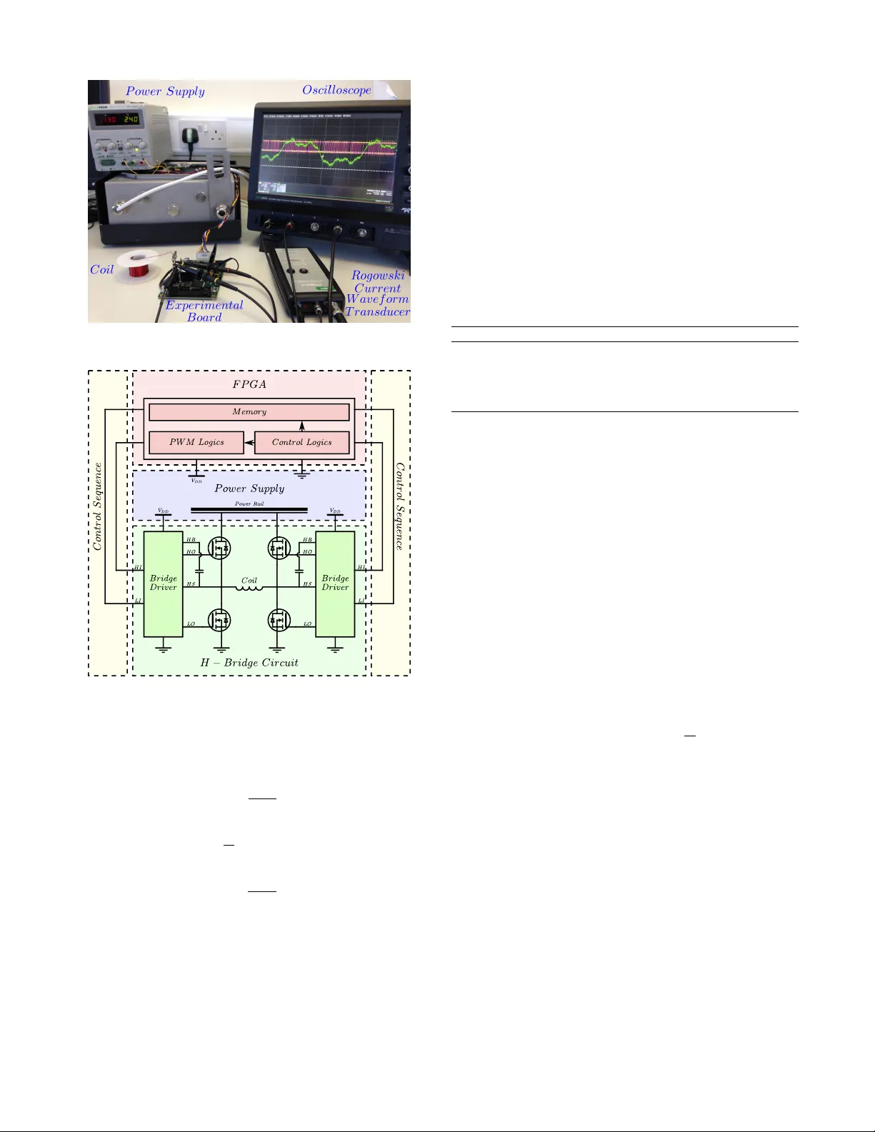
IEEE TRANSACTIONS ON INDUSTRIAL ELECTR ONICS A Class D P o wer Amplifier f or Multi-F requency Eddy Current T esting Based on Multi-Simultaneous-F requency Selectiv e Har monic Elimination Pulse Width Modulation Y ang T ao, Member , IEEE, Christos Ktistis, Yif ei Zhao , Wuliang Y in, Senior Member , IEEE, and Anthony J . P e yton Abstract —Efficiency and m ultisimultaneous-frequency (MSF) output capability are two major criteria characteriz- ing the perf ormance of a power amplifier in the application of multifrequenc y eddy current testing (MECT). Switch- mode power amplifiers are known to have a very high effi- ciency , yet they have rarel y been adopted in the instrumen- tal development of MECT . In addition, switch-mode power amplifiers themselves are lacking in the research literature for MSF capability . In this ar ticle, a Class D power amplifier is designed so as to address the tw o issues. An MSF selec- tive harmonic elimination pulsewidth modulation method is proposed to generate alternating magnetic fields, which are rich in selected harmonics. A field-programmable-gate- array-based experimental system has been developed to verify the design. Results show that the proposed method- ology is capable of g enerating high MSF currents in the transmitting coil with a low distortion of signal. Index T erms —Class D power amplifier , edd y current, m ul- tifrequency , pulsewidth modulation (PWM), selective har- monic elimination. I . I N T R O D U C T I O N M UL TI-FREQUENCY eddy current testing (MECT) has attracted increasing attention for non-destructiv e test- ing (NDT) in recent years. In comparison with the single- frequency eddy current method, MECT tak es advantage of wide-band spectral signals, which is advantageous for applica- tions such as detecting cracks in conducti ve materials [1], mea- suring thickness of metal film [2], monitoring microstructure in steel production [3] and imaging conductivity profile of metal structures [4], etc. In these applications of MECT , a high- current po wer amplifier with multi-simultaneous-frequency (MSF) output capability is indispensable in the signal chain so as to achie v e high o verall sensitivity [5]. Manuscript received March 22, 2019; revised July 17, 2019 and September 2, 2019; accepted October 8, 2019.This work was suppor ted by the U.K. Engineer ing and Physical Sciences Research Council via the University of Manchester Impact Accelerator Account under Grant EP/R511626/1. (Corresponding author: Y ang T ao; Wuliang Yin.) The authors are with the Depar tment of Electrical and Electronic En- gineering, School of Engineering, The Univ ersity of Manchester , Manch- ester M13 9PL, U.K. (e-mail: yang.tao@manchester .ac.uk; christos. ktistis@manchester .ac.uk; yifei.zhao@manchester .ac.uk; wuliang.yin@ manchester .ac.uk; a.peyton@manchester .ac.uk). Color versions of one or more of the figures in this article are av ailable online at http://ieeexplore .ieee.org. Digital Object Identifier 10.1109/TIE.2019.2947842 Class D power amplifier has the virtue of high current handling capacity and power ef ficiency [6], [7]. Ho wev er , transmitting signals may suf fer severe distortion after amplifi- cation if they are not modulated properly . A notable category of modulation methods is known as the programmed pulse width modulation (PPWM) or selectiv e harmonic elimination pulse width modulation (SHEPWM) [8] which has drawn tremendous interests and been studied primarily for high- power high-voltage con verters [9]. Owing to the lack of motiv ation of generating multi-simultaneous frequencies using SHEPWM, ef forts ha ve been mainly dev oted in a manner to achiev e varying outputs of the fundamental component which is characterised by the modulation index and to eliminate the remaining harmonics. Y et in MECT applications, the varying modulation inde x is not of interest while the MSF output capability is of importance. Therefore, some harmonics may be well harnessed rather than eliminated. This paper attempts, for the first time, to e xamine the MSF capability of the SHEPWM technique and in addition, to introduce switch-mode power amplifier into the instru- mental development of MECT . A Class D power amplifier based upon multi-simultaneous-frequency SHEPWM (MSF- SHEPWM) is designed. The proposed design is capable of driving an excitation coil with a simultaneous multi-frequency signal. Moreo ver , it is con v enient to change the spectrum of the transmitting signal. Experimental results have proved that the system could transmit MSF alternating magnetic fields with low distortion. The remainder of the paper is organised as follows. Section §II describes the principle of MSF-SHEPWM. The design of hardware and the results of experiments are presented in Section §III. Finally , conclusions are drawn in the last section. I I . M S F - S H E P W M P R I N C I P L E In eddy current testing, the load of the po wer amplifier is a coil that generates alternating magnetic fields. In order to generate the magnetic fields that are required for MECT , according to the Amp` ere 0 s law , we can directly design the current through the coil. The wav eform of coil current is a concatenation of a fe w straight line se gments of fix ed gradients when the coil is connected to a Class D power amplifier . This is due to the fact that in theory the voltage across the coil IEEE TRANSACTIONS ON INDUSTRIAL ELECTR ONICS can only ha ve a fixed number of values or lev els and, for a perfect inductor , the coil current is an integral of the voltage. Figure 1 shows three example topologies for Class D power amplifier . Enhancement-mode n-type MOSFETs are used for this illustration. The components in blue colour constitute a conducting path. Figure 1(a) shows a push-pull configuration where the voltage across the coil have two le vels, i.e. + V DC / 2 and − V DC / 2 ; Figure 1(b) depicts a full H-bridge topology that is capable of driving the coil with three-lev el voltage, i.e. + V DC , 0 and − V DC . Multi-level voltage can be achiev ed by utilising multiple full H-bridges. For example, a fiv e-lev el in verter is shown in Figure 1(c) that contains two H-bridge cells. The fiv e values of voltage are +2 V DC , + V DC , 0 , − V DC and − 2 V DC . Fig. 1. T opology of Class D power amplifier using enhancement-mode n-type MOSFETs. (a) push-pull half bridge. (b) full H-bridge. (c) two full H-bridges. The objectiv e of MSF-SHEPWM is to generate an output wa veform that contains the desired MSF spectral components, but eliminates the unwanted harmonics. The principle of MSF-SHEPWM can be summarised in three stages. Firstly , the objectiv e signal is synthesised based on the fundamental sinusoidal signal and a few harmonics in the time domain, and the wa veform of the synthesised signal is resembled by straight line segments in a morphological sense. Secondly , the resultant resemblance signal is decomposed as Fourier series and analysed in the frequency domain. Finally , the Fourier coefficients are adjusted by solving an optimisation problem. These three stages will no w be described in detail in the following sub-sections. For clarity we use f k ( t ) to denote the objectiv e signal, g k ( t ) as the resemblance function of f k ( t ) , and G k ( t ) is the Fourier series of g k ( t ) . The subscript k refers to a specific signal. A. Synthesis of the objective function f k ( t ) in the time domain A periodic signal f ( t ) that contains n sinusoidal basic components is expressed as (1) where ω p , θ p and w p are the angular frequency , phase angle and coefficient of the p th component respectively . The function f ( t ) serves as the objectiv e coil current that is to be generated and the coefficient w p forms the amplitude spectrum. Additionally , three conditions are exerted on f ( t ) . Firstly , the lowest frequency is set as the fundamental frequency ω and higher frequencies are harmonics of ω , i.e. ω p = pω . This is a natural requirement since the signal generated by Class D po wer amplifier is rich in harmonics. Secondly , the phase angle θ p is zero implying all the basic components are in-phase. In MECT applications, the relativ e phase values are not critical factors. Thirdly , the coefficient w p is chosen as 1 p for the selected frequencies and zero for absent harmonics. In general, the magnitude of response signal tends to increase with frequency . In order to achie ve similar signal-to-noise ratio (SNR) in the whole spectrum of interest, the coefficient w p is chosen to be inv ersely proportional to the frequency ω p or the order p . In fact, (1) is a special case of the trigonometric form of Fourier series but only a few rather than an infinite number of components are in volv ed. f ( t ) = n X p =1 w p sin ( ω p t + θ p ) (1) f 1 ( t ) = sin ( ωt ) + 1 3 sin (3 ωt ) + 1 9 sin (9 ωt ) + 1 27 sin (27 ωt ) + 1 81 sin (81 ωt ) (2) f 2 ( t ) = sin ( ωt ) + 1 3 sin (3 ωt ) + 1 7 sin (7 ωt ) + 1 17 sin (17 ωt ) (3) f 3 ( t ) = sin ( ωt ) + 1 2 sin (2 ωt ) + 1 4 sin (4 ωt ) + 1 6 sin (6 ωt ) + 1 8 sin (8 ωt ) + 1 10 sin (10 ωt ) + 1 12 sin (12 ωt ) + 1 14 sin (14 ωt ) (4) f 4 ( t ) = sin ( ωt ) + 1 2 sin (2 ωt ) + 1 3 sin (3 ωt ) + 1 4 sin (4 ωt ) + 1 5 sin (5 ωt ) + 1 6 sin (6 ωt ) + 1 7 sin (7 ωt ) + 1 8 sin (8 ωt ) (5) f 5 ( t ) = sin ( ωt ) + 1 3 sin  3 ω t + π 4  + 1 9 sin  9 ω t + π 7  + 1 27 sin  27 ω t + π 5  + 1 81 sin  81 ω t + π 6  (6) As an example, a signal f 1 ( t ) that follows these principles is shown in Figure 2. Here, f 1 ( t ) is a superposition of five basic sinusoidal signals. The frequencies are chosen in a geometric scale as ω , 3 ω , 9 ω , 27 ω and 81 ω . The weights are set as 1 , 1 3 , 1 9 , 1 27 , and 1 81 . Another three examples f 2 ( t ) , f 3 ( t ) and f 4 ( t ) that have different possible combinations of basic components are shown in Figure 3. The expressions of f 1 ( t ) , f 2 ( t ) , f 3 ( t ) and f 4 ( t ) are shown in (2), (3), (4) and (5), respectively . The selection of inv olving harmonics has flexibility and is determined by the fundamental frequency and the spectrum IEEE TRANSACTIONS ON INDUSTRIAL ELECTR ONICS Angle (rads) Function V alue 1.2 0 -1.1 Foundamental Harmonic 0 Harmonic Harmonic Harmonic Fig. 2. The objectiv e function f 1 ( t ) , the corresponding fundamental and harmonic functions of interest. The associated coefficients are determined by the requirement of power distribution for each harmonics. It should be noted that the basic sinusoidal components do not necessarily have to be in-phase relati ve to each other . For example, f 5 ( t ) as expressed in (6), has the same weights for each basic components as f 1 ( t ) , but the phases are different which is shown in Figure 3. Although f 5 ( t ) has the same amplitude spectrum as f 1 ( t ) , some symmetric features are broken which makes the analysis in the frequenc y domain more complicated. Function V alue 1.8 -1.8 0 0 Angle (rads) Fig. 3. Objective function: f 1 ( t ) , f 2 ( t ) , f 3 ( t ) , f 4 ( t ) and f 5 ( t ) Once the waveform of the objective function is determined, such wav eform can be resembled using straight line segments as shown in Figure 4. The resemblance function g ( t ) is piece- wise linear with different gradients and approximates the objectiv e function f ( t ) . Accurate approximation requires mul- tiple lev els of output voltage which, howe ver , costs multiple H-bridge cells. Therefore, the selection of voltage lev els is a trade-off between the fidelity of signal and feasibility in practice. The number of time steps used for g ( t ) is often determined by the clock frequency used to driv e the bridge circuit and limited by the dynamic characteristics of the transistor . B. Analysis of the resemblance function g k ( t ) in the fre- quency domain 1) Calculation of the F ourier coef ficients for the resem- blance function g k ( t ) : A resemblance function g k ( t ) can be generated by a multi-le vel Class D power amplifier . The Function V alue 0 0 1.1 Angle (rads) Fig. 4. An objective function f ( t ) and its resemblance function g ( t ) switching scheme in a quarter period is depicted in Figure 5. Switching angles satisfy 0 ≤ α 1 ≤ α 2 ≤ · · · ≤ α N ≤ π 2 and at each angle the voltage can raise or fall by V 0 until reaching the limits. The coil current is essentially an integral of the pulse v oltage which is depicted as the area in the magenta colour in Figure 5. Therefore, the Fourier series of the coil current is calculated as (7). The Fourier coefficient is shown in (8) which is a function of N switching angles α q , the coil inductance L , the order of harmonics p and the step of voltage V 0 . Fig. 5. Switching scheme of multi-lev el Class D amplifier G ( t ) = ∞ X p =1 , 3 , ··· b p sin ( pωt ) (7) b p = − 4 V 0 p 2 π ω L N X q =1 ( − 1) s sin ( pα q ) , s = ( 1 , ∀ α q at w hich ther e is a f al ling edg e 0 , ∀ α q at w hich ther e is a r aising edge (8) C . Optimisation of the Fourier coefficients b p Once the wa veform of the resemblance function g k ( t ) is obtained based on the gradient of f k ( t ) , the spectrum of g k ( t ) can be controlled by adjusting the switching angles α q which is essentially a problem of solving simultaneous transcendental equations. Each equation corresponds to the magnitude of a harmonic to be controlled. IEEE TRANSACTIONS ON INDUSTRIAL ELECTR ONICS V arious methods hav e been de veloped in order to obtain one or multiple solutions to the harmonic magnitude equa- tions. One direction for developing a solver is based on the elimination theory of polynomial and using the r esul tant [10]. Unfortunately , the order of polynomials increases with the number of harmonics to be controlled which results in a significant computational burden if the application entails a wide spectrum. Moreov er , completely solving the equations might be a stringent requirement and in f act discrepancies could be tolerated within a threshold in a real application. Another direction tends to recast the harmonic magnitude equations into an optimisation problem [8]. Because of the trigonometric and non-con vex nature of the harmonic mag- nitude equations, it is difficult to guarantee that a globally optimal solution can be achie ved. Meta-heuristic algorithms such as differential e volution [11], genetic algorithm [12], and particle swarm optimisation [13], etc. hav e been applied to obtain a global solution through modern stochastic search techniques. Howe v er , different results may be returned for the same problem since these algorithms rely on random searches. Many gradient based algorithms, on the other hand, guarantee that a local optimal can be obtained in theory . If a good estimation of the solution exists, the gradient based algorithms could con ver ge to the optimal rapidly [14]. min 0 ≤ α 1 ≤ α 2 ≤···≤ α N ≤ π 2 ,m p X p ∈ Φ λ p  pω L V 0 b p − m p  2 , subj ect to     pω L V 0 b p     ≤  p , ∀ p ∈ Ψ (9) In this paper, the harmonic magnitude equations are calcu- lated by solving a constrained nonlinear optimisation problem as shown in (9). Follo wing the conv ention of multi-level in verter , we denote the modulation index for the p th harmonic frequency as m p = V p V 0 , where V p is the amplitude of the p th harmonic in the output voltage. The modulation index characterises the relati ve amplitude of output voltage in the context of a multi-le vel in verter , b ut there are two different considerations for MECT . Firstly , m p is of interest for multiple harmonics, yet only the fundamental frequency component is relev ant for a multi-le vel in verter . Secondly , m p is treated as an optimising parameter , while a multi-le vel in verter tends to be able to output a range of values of the modulation index. In (9), Φ is a set whose elements are the orders of selected harmonics while the elements of Ψ are the orders of harmonics to be eliminated. The objectiv e function in (9) represents the sum of weighted ( λ p ) squared residuals of the modulation index for selected harmonics subject to such constrains that the modulation index of undesirable harmonics is bounded with threshold  p . The optimising parameters are N switching angles α 1 , α 2 , · · · , α N and the modulation index m p . The problem (9) could provide many flexibilities in prac- tice. For instance, the adjacent harmonics of an objective frequency will cause interference at that frequency and hence the corresponding threshold  p for the adjacent harmonics should be smaller than those of other less critical harmonics. Additionally , if annulation of the objecti ve function is not possible, the objectiv e function could be relaxed by putting higher weights λ p for more important harmonics and lower weights for other harmonics. The interior-point algorithm is adopted to solve the problem (9). This choice of algorithm is due to the fact that the interior-point algorithm has been proved to be an effecti ve solver for constrained nonlinear optimisation problems [15]. Moreov er , both the objectiv e function and constrain function hav e well-defined Gradient and Hessian. Besides, the initial value of switching angles can be obtained based on the gradient of objectiv e function f ( t ) which turns out to be a good estimation. The M AT LAB r O ptimiz ation T oolbox r provides a solver fmincon that implements the interior-point algorithm. I I I . H A R D WA R E A N D E X P E R I M E N TAL R E S U L T S A. Hardware Implementation In order to test the proposed MSF-SHEPWM method, an FPGA based experimental system was designed which is shown in Figure 6. The system schematic diagram is shown in Figure 7. The system mainly comprises three parts, namely a S partan r − 6 FPGA, power supply and H-bridge circuit. An oscillator on the experiment board generates a clock signal of a fixed frequency , and a digital clock manager (DCM) inside the FPGA is used to generate a specified baseline clock signal for control sequence. The FPGA periodically reads the switching sequence from in-chip memory and outputs pulse signals through a PWM logic block. The pulse signals are then fed into the bridge driv er . Four enhancement-mode n- type MOSFETs are utilised in the system configured in a full H-bridge. Therefore, three lev els of voltage can be generated by the H-bridge cell. According to the analysis of two cases of application that will be shown in the following paragraphs, ev en a bipolar pulse voltage is sufficient in generating the de- sired magnetic fields. Although the proposed MSF-SHEPWM method applies to the design of multiple H-bridge cells, only a single full H-bridge is adopted in the system. In order to make the enhancement-mode n-type MOSFETs working in the ohmic region, the gate-to-source voltage must be higher than not only the threshold voltage, but the addition of the drain-to-source voltage and the threshold voltage. Therefore, a bootstrap circuit is required to dri ve the high side MOSFETs. The dc voltage is selected as 24 V supplied externally . B. P ower and Efficiency Metrics The drain efficienc y η [16] as expressed in (10) is adopted as an efficienc y metric, in which the input dc power P DC is the product of the dc po wer supply voltage V DC and current I DC . The real output power P out is defined in (11), in which u out , i out and T are the load voltage, current and integration interv al, respectiv ely . As the objectiv e is generating ac magnetic field rather than dissipating dc power in the load, we define an energy con version factor ζ as (12), in which the output reactiv e po wer Q out [17] is defined as (13) where U i and I i are the root-mean-squared values of the output voltage and current harmonics of order i . θ i is the phase angle IEEE TRANSACTIONS ON INDUSTRIAL ELECTR ONICS Fig. 6. Exper imental system Fig. 7. Schematic diagram of the experimental system difference between them, and Ψ is the set containing the orders of transmitting harmonics. η = P out P DC (10) P out = 1 T Z T u out i out d t (11) ζ = Q out P DC (12) Q out = X i ∈ Ψ U i I i sin θ i (13) C . T wo Experiments The selection of e xcitation frequencies is of high importance and it can be expected that dif ferent spectrum is required for different applications. For example, the β − disper sion frequency range from hundreds of kilohertz to megahertz is often harnessed to detect the property which relates to the cellular structure of biological tissues [18], while 20 k H z to 100 k H z is a suitable range for measuring copper film with thickness of 10 – 400 µm [19]. T wo experiments are carried out based on the experimental system. In the first experiment, the full design procedures are illustrated and the questions needing attentions are discussed. In the second experiment, we sho w a fast design without the procedure of analysing in the frequency domain and the optimisation process. The setups of two experiments can be found in T able I. T ABLE I D E TAI L E D S E T U P S O F T W O E X P E R I M E N T S Experiment No. 1 Experiment No. 2 Selected Harmonics 1 st , 3 rd , 7 th , 17 th 1 st , 3 rd , 9 th , 27 th , 81 st Clock Frequency 24 M H z 6 . 25 M H z Lookup Table Length 476 bits 3888 bits Transmitting Frequency 50 . 42 kH z , 151 . 26 k H z , 352 . 94 kH z , 857 . 14 k H z 1 . 61 kH z , 4 . 82 k H z , 14 . 47 kH z , 43 . 40 kH z , 130 . 21 k H z Coil Inductance 1 . 4 µH 662 µH Wire Diameter (A WG) 13 AW G 26 AW G 1) Experiment No. 1: The objectiv e of this experiment is to generate high currents for a lo w-impedance coil in the frequency range between 10 k H z and 1 M H z . T est samples can be transferred through the aperture of the coil. This configuration could be applied to inline discrimination of metal contaminants, grading of food product and monitoring of meat ageing process, etc. a) Excitation fr equencies: Deciding the number of trans- mitting frequencies is a trade-off between power distribution and spectral resolution. If too many frequencies are selected, it’ s inevitable that the power will be relati vely low for an individual frequency . Moreov er , if two selected frequencies are too close, not enough distinction of the response signal could be drawn from them. As a result, four frequencies are chosen for this experiment as the fundamental, 3 rd , 7 th and 17 th harmonics which results in the earlier mentioned objective function f 2 ( t ) in II-A. The clock frequency is configured as 24 M H z and the highest frequency is 1 28 of the clock fre- quency . Therefore, the four transmitting frequencies are about 50 . 42 k H z , 151 . 26 k H z , 352 . 94 k H z and 857 . 14 k H z . It is noted that these frequencies well span the objectiv e spectrum but are relativ ely arbitrary and the transmitting frequencies could be altered by either changing the clock frequency or the ratio of the highest frequency over the clock frequency . b) Levels of output voltage: Determining the number of output voltage le vels of the amplifier is another trade-off. As shown in Figure 8, the resemblance function g 2 ( t ) generated by the bipolar voltage across the coil is able to approximate the objecti ve function f 2 ( t ) with a tolerable error in practice. It will be justified through practical test that the bipolar output voltage is capable of generating the coil currents with low distortion. In addition, there are only six switching angles α 1 , α 2 , α 3 , α 4 , α 5 and α 6 in a quarter period. The highest switching frequency is close to the 17 th harmonic frequency implying that the magnitude of the harmonic frequencies higher than the highest transmitting frequency will be low . Therefore, a low-pass filter is no longer needed. IEEE TRANSACTIONS ON INDUSTRIAL ELECTR ONICS Pulse V oltage and Sca led Current 0 43 129 215 301 387 476 Clock Cycle V oltage 0 Fig. 8. f 2 ( t ) , g 2 ( t ) and the pulse voltage that gener ates g 2 ( t ) c) Setup of optimisation pr oblem: According to (8) the Fourier coefficients b p of g 2 ( t ) can be calculated as (14). Cautions should be made that there are two falling edges, i.e. + V DC to 0 and 0 to − V DC at α 1 , α 3 , α 5 , two raising edges, i.e. − V DC to 0 and 0 to + V DC at α 2 , α 4 , α 6 , and one falling edge, i.e. + V DC to 0 at π 2 . Substituting (14) in (9) giv es rise to the optimisation problem (15) where the dc voltage V DC and coil inductance L hav e been cancelled. Additionally , because we would like b p to be in versely proportional to p , (15) is in fact normalised where each residual in the objectiv e function should have similar lev el of magnitude. b p = − 4 V DC p 2 π ω L 2 6 X q =1 ( − 1) q sin ( pα q ) − sin  pπ 2  ! , p = 1 , 3 , 5 , · · · (14) The initial values of the six switching angles are the points where the gradient of f 2 ( t ) is zero as shown in Figure 8. The angles can only have discrete values and the resolution is determined by the product of the order of the highest harmonic and the ratio of the clock frequency over the highest transmitting frequency . As a result, the length of the lookup table which stores the control sequence is 476 as a product of 17 and 28 and hence the resolution of angle is 2 π 476 r ads . Since every switching angle is an integer multiplied by the resolution, it is conv enient to use the number of clock cycle to represent the angles. A set of initial values is listed in the first row of T able II. These initial values are substituted into (14) in order to calculate the modulation index m p . The objectiv e b p of selected harmonics is inv ersely proportional to p , so the corresponding modulation index m p should have the same value. As a result, the average value of m 1 , m 3 , m 7 and m 17 when substituting the initial angles is used as the initial value for m 1 , m 3 , m 7 and m 17 . The constrain threshold  p is set up in a way that the scaled modulation index m p p for those undesirable harmonics has the same bound. The modulation index m p is scaled by p because we would like b p to hav e the same bound for undesirable harmonics. All the weights λ p are configured as one for the first setup and then the residual of the 17 th harmonic is relaxed by setting λ 17 as zero which is the second setup. The reason of such relaxation will be discussed in following paragraphs. Details of the initial condition and two setups for the parameters are listed in T able II. d) Results: The optimisation problem (15) giv en the initial condition under two setups of parameters is solved using the interior-point algorithm. The resultant switching angles, total harmonic distortion (THD) and scaled modulation index m p p are listed in T able II where the THD is defined as (16). Here we use m p p to represent b p because the former is independent of the coil inductance L while the latter is not. An Fast Fourier T ransform (FFT) is conducted to the resemblance functions when the initial switching angles, the optimal angles of the first setup and of the second setup are applied. The results are plotted in Figure 9. T H D = q P p ∈ Ψ b 2 p q P p ∈ Φ b 2 p × 100 % (16) It can been seen from T able II that the initial switching angles already lead to a low THD of 7 . 33 % . Howe ver , the power distribution among the four selected frequencies is not the same as desired. The fourth component is higher while the second and third component are lo wer than they should be. This situation is improved by the optimisation under the first setup. Equal weights are assigned to the four residuals resulting in a more desirable power distribution. Howe ver , the THD has been increased to 9 . 04 % which is mainly caused by the increase of the adjacent harmonic components of 857 . 14 k H z that can be seen in Figure 9. The reason behind this is that initially the frequency of the highest-frequency ripple is close to 857 . 14 k H z which in turn gives rise to the large component of 857 . 14 k H z and a clean spectrum higher than 857 . 14 k H z . The optimisation process tends to penalise the residual of 857 . 14 k H z by , unfortunately , increasing its adjacent harmonic components rather than the lower desirable harmonics. Consequently , it is reasonable to always relax the penalty of the ’ benig n r ippl e ’ as has been done in the second setup. As sho wn in T able II, the scaled modulation index of the first three frequencies have a better ratio comparing to those of the first optimisation while the highest-frequency m p p and THD are similar . The wa veforms of the associated resemblance functions for the three sets of switching angles are shown in Figure 10. The optimal switching angles of the second optimisation setup are implemented in the experimental system to drive a coil with an inductance of about 1 . 4 µH . The screenshot of an oscilloscope displaying the coil current and bipolar output voltage is shown in Figure 11. The peak-to-peak value of the current through the coil is higher than 60 A . An FFT is done to the current and the largest ten root-mean-square (RMS) v alues and the corresponding frequencies are listed in T able III. 2) Experiment No. 2: Compared to the first experiment, the objecti ve of the second experiment is to drive a higher- impedance coil in a lower spectrum from about 1 k H z to 200 k H z . The axis of the coil aperture would point to the test samples. Application of this spectrum can be found in the inspection of welding process, crack detection of metal samples and thickness measurement of metal film, etc. IEEE TRANSACTIONS ON INDUSTRIAL ELECTR ONICS min 0 ≤ α 1 ≤ α 2 ≤···≤ α 6 ≤ π 2 ,m p X p =1 , 3 , 7 , 17 λ p 8 pπ 6 X q =1 ( − 1) q sin ( pα q ) − 4 pπ sin  pπ 2  + m p ! 2 , subj ect to      8 pπ 6 X q =1 ( − 1) q sin ( pα q ) − 4 pπ sin  pπ 2       ≤  p , ∀ p ∈ { 5 , 9 , 11 , 13 , 15 } (15) T ABLE II R E S I D U A L W E I G H T λ p , C O N S T R A I N T H R E S H O L D  p , S W I T C H I N G A N G L E α q , S C A L E D M O D U L ATI O N I N D E X m p p A N D T H E TO T A L H A R M O N I C D I S TO R T I O N F O R T H E I N I T I A L A N D T W O O P T I M I S A T I O N S E T U P S O F E X P E R I M E N T N O . 1 λ 1 λ 3 λ 7 λ 17  5  9  11  13  15 Switching angle (clock cycle) m p p T H D (%) α 1 α 2 α 3 α 4 α 5 α 6 50 . 42 k H z 151 . 26 k H z 352 . 94 k H z 857 . 14 k H z Initial − − − − − − − − − 36 49 68 77 88 111 0 . 534 0 . 145 0 . 066 0 . 043 7 . 33 No. 1 1 1 1 1 0 . 10 0 . 18 0 . 22 0 . 26 0 . 30 39 51 70 82 90 111 0 . 553 0 . 171 0 . 047 0 . 032 9 . 04 No. 2 1 1 1 0 0 . 10 0 . 18 0 . 22 0 . 26 0 . 30 35 48 65 74 86 111 0 . 493 0 . 157 0 . 068 0 . 043 7 . 80 Scaled Modula tion Index 0 0 0.1 0.2 0.3 0.4 0.5 0.6 50.42 151.26 252.10 352.94 453.78 554.62 655.46 756.30 857.14 957.98 1059 1 160 1261 Initial Optimal No. 1 Optimal No. 2 Frequency Fig. 9. Scaled modulation index m p p with respect to frequency for the initial switching angles, optimal angles of the first setup and the second setup of experiment No .1 Initial Optimal No. 1 Optimal No. 2 Scaled Current Clock Cycle 0 0 -1 1 1 19 238 357 476 Fig. 10. Wa vef orm of the resemblance function for the initial switching angles, optimal angles of the first setup and the second setup of experiment No .1 The objecti ve function f 1 ( t ) , as shown in Figure 12, is implemented in this experiment where the fundamental, 3 rd , 9 th , 27 th and 81 st harmonics are inv olved. The resemblance function g 1 ( t ) is also plotted in Figure 12 and there are 38 switching angles in a quarter period of g 1 ( t ) . Because the highest order harmonic is the 81 st harmonic, g 1 ( t ) requires more switching angles than g 2 ( t ) . The initial values of the switching angles are determined in the same way as it is in Fig. 11. Coil current (green trace), output voltage of one half bridge (yello w trace) and of the other half br idge (red trace) for optimisation No . 2 of experiment No . 1 T ABLE III F F T R E S U L T S O F T H E C O I L C U R R E N T F O R O P T I M I S A T I O N N O . 2 O F E X P E R I M E N T N O . 1 No. Frequenc y Current (RMS) No. Frequency Current (RMS) 1 50 . 42 kH z 16 . 97 A 6 554 . 62 kH z 0 . 76 A 2 151 . 26 kH z 6 . 15 A 7 252 . 10 kH z 0 . 49 A 3 352 . 94 kH z 2 . 08 A 8 1462 . 18 kH z 0 . 49 A 4 857 . 14 kH z 1 . 49 A 9 756 . 30 kH z 0 . 32 A 5 655 . 46 kH z 0 . 81 A 10 453 . 78 kH z 0 . 31 A the first experiment, i.e. examining the gradient of objectiv e function. The clock frequency is configured as 6 . 25 M H z and the fiv e transmitting frequencies are chosen as about 1 . 61 k H z , 4 . 82 k H z , 14 . 47 k H z , 43 . 40 k H z and 130 . 21 kH z . As a result, the memory needs 3888 bits to store the control sequence. In order to show that a fast design could be done without the optimisation process discussed in the first experiment, the initial values of the 38 switching angles are directly implemented in the experimental system. The screenshot of an oscilloscope displaying the coil current and bipolar output voltage is shown in Figure 13. The peak-to-peak value of the current through the coil is about 2 . 5 A . An FFT is done to the current and the largest ten root-mean-square (RMS) values and IEEE TRANSACTIONS ON INDUSTRIAL ELECTR ONICS the corresponding frequencies are listed in T able IV. V oltage Pulse V oltage and Sca led Current Clock Cycle 0 0 500 1000 1500 2000 2500 3000 3500 3888 Fig. 12. f 1 ( t ) , g 1 ( t ) and the pulse voltage that gener ates g 1 ( t ) Fig. 13. Coil current (green trace), output voltage of one half bridge (yello w trace) and of the other half bridge (red trace) for e xperiment No. 2 T ABLE IV F F T R E S U L T S O F T H E C O I L C U R R E N T F O R E X P E R I M E N T N O . 2 No. Frequency Current (RMS) No. Frequency Current (RMS) 1 1 . 61 kH z 751 . 46 mA 6 8 . 04 kH z 10 . 53 mA 2 4 . 82 kH z 284 . 49 mA 7 20 . 90 k H z 10 . 30 mA 3 14 . 47 kH z 89 . 05 mA 8 11 . 25 k H z 7 . 75 mA 4 43 . 40 kH z 24 . 60 mA 9 17 . 68 k H z 7 . 52 mA 5 130 . 21 k H z 22 . 80 mA 10 27 . 33 k H z 5 . 49 mA 3) P ower and efficiency comparison between two experi- ments: According to (10), (11), (12) and (13), the power and efficienc y metrics of the two experiments are calculated and listed in T able V. In terms of the efficienc y η , the first experiment has a lo wer value of 20.02%, which is due to the fact that the coil has a high quality factor and much of the power is dissipated by the MOSFETs. In contrast, the efficienc y η is 76.92% in the second experiment, because the coil is lossy . The energy con version factor ζ is larger than unity for both experiments. The reactive power Q out for the first experiment is as large as 224.81 v ar with a total dissipated power of 34.32 W . The second experiment has a lo wer ζ mainly because of its higher impedance of the coil. If possible, we would pursue a low ef ficiency η , because power dissipation in the load would be a waste of energy . On the other hand, a large energy con v ersion factor ζ is preferred, which implies that an ac magnetic field would be generated while consuming low dc power . T ABLE V P O W E R A N D E FFI C I E N C Y M E T R I C S O F T W O E X P E R I M E N T S . Experiment V DC I DC P DC P out Q out η ζ No. 1 24.00 V 1.43 A 34.32 W 6.87 W 224.81 var 20.02% 6.55 No. 2 24.00 V 0.13 A 3.12 W 2.40 W 8.62 var 76.92% 2.76 I V . C O N C L U S I O N S The instrumental development of MECT entailed a highly efficient amplifier in the transmitting power stage. Switch- mode po wer amplifiers exhibited compelling adv antages in terms of efficiency . This article attempted to serve as a bridge that introduced a switch-mode power amplifier into the design of MECT instrumentation. Being able to transmit MSF magnetic fields was critical in MECT but was not a primary goal in the research of modulation strategy of switch-mode amplifiers or con verters. Hence, this article also examined the MSF capability of the SHEPWM technique. A Class D power amplifier was developed in this article aiming at gen- erating high MSF currents in the transmitting coil. An MSF- SHEPWM method was proposed to modulate the pulse voltage across the coil. Three concise steps could summarize the new modulation strategy , i.e., time-domain synthesis of harmonic signals, frequency-domain analysis of the resemblance signal, and optimisation of the resultant Fourier coefficients. An FPGA-based experimental system was developed, and the proposed methodology was implemented in two experiments. The first experiment transmitted magnetic fields exciting at four simultaneous frequencies with a THD as low as 8%. The peak-to-peak value of the coil current was as high as 60A while the total power dissipation was low .The size of the circuit board was small and no large heat dissipating facilities were needed. The second experiment tries to illustrate a fast design process showing that the proposed method was still effecti v e even with the first step only . Fi ve frequencies were transmitted in a smaller span of spectrum comparing to the first experiment. The two experiments ha ve shown that the design is versatile and could be applied to different electromagnetic inductiv e sensing scenarios. A C K N O W L E D G E M E N T All research data supporting this publication are directly av ailable within this publication. R E F E R E N C E S [1] A. Bernieri, G. Betta, L. Ferrigno, and M. Laracca, “Crack Depth Esti- mation by Using a Multi-Frequency ECT Method, ” IEEE Tr ansactions on Instrumentation and Measurement , vol. 62, no. 3, pp. 544–552, Mar. 2013. [2] W . Yin and A. J. Peyton, “Thickness measurement of non-magnetic plates using multi-frequency eddy current sensors, ” NDT & E Interna- tional , vol. 40, no. 1, pp. 43–48, Jan. 2007. [3] S. Johnstone, R. Binns, A. J. Peyton, and W . D. Pritchard, “Using electromagnetic methods to monitor the transformation of steel samples, ” T ransactions of the Institute of Measurement and Control , vol. 23, no. 1, pp. 21–29, Mar . 2001. IEEE TRANSACTIONS ON INDUSTRIAL ELECTR ONICS [4] W . Y in, S. Dickinson, and A. Peyton, “Imaging the continuous con- ductivity profile within layered metal structures using inductance spec- troscopy , ” IEEE Sensors Journal , vol. 5, no. 2, pp. 161–166, Apr . 2005. [5] J. García-Martín, J. Gómez-Gil, and E. Vázquez-Sánchez, “Non- Destructiv e T echniques Based on Eddy Current T esting, ” Sensors , vol. 11, no. 3, pp. 2525–2565, Feb. 2011. [6] J. Rodriguez, J.-S. Lai, and F . Z. Peng, “Multilevel in verters: a survey of topologies, controls, and applications, ” IEEE T ransactions on Industrial Electr onics , vol. 49, no. 4, pp. 724–738, Aug. 2002. [7] M. Malinowski, K. Gopakumar , J. Rodriguez, and M. Pérez, “ A Survey on Cascaded Multilevel In verters, ” IEEE T ransactions on Industrial Electr onics , vol. 57, no. 7, pp. 2197–2206, Jul. 2010. [8] M. S. A. Dahidah, G. Konstantinou, and V . G. Agelidis, “ A Review of Multilev el Selecti ve Harmonic Elimination PWM: Formulations, Solving Algorithms, Implementation and Applications, ” IEEE T ransactions on P ower Electronics , vol. 30, no. 8, pp. 4091–4106, Aug. 2015. [9] J. Napoles, J. I. Leon, R. Portillo, L. G. Franquelo, and M. A. Aguirre, “Selectiv e Harmonic Mitigation T echnique for High-Power Conv erters, ” IEEE T ransactions on Industrial Electronics , vol. 57, no. 7, pp. 2315– 2323, Jul. 2010. [10] J. N. Chiasson, L. M. T olbert, K. J. McKenzie, and Z. Du, “Control of a multilev el con verter using resultant theory , ” IEEE T ransactions on Contr ol Systems T echnology , vol. 11, no. 3, pp. 345–354, May . 2003. [11] A. M. Amjad, Z. Salam, and A. M. A. Saif, “ Application of differential ev olution for cascaded multilevel VSI with harmonics elimination PWM switching, ” International J ournal of Electrical P ower & Ener gy Systems , vol. 64, pp. 447–456, Jan. 2015. [12] S. S. Lee, B. Chu, N. R. N. Idris, H. H. Goh, and Y . E. Heng, “Switched- Battery Boost-Multilev el In verter with GA Optimized SHEPWM for Standalone Application, ” IEEE Tr ansactions on Industrial Electr onics , vol. 63, no. 4, pp. 2133–2142, Apr . 2016. [13] H. T aghizadeh and M. T . Hagh, “Harmonic Elimination of Cascade Multilev el Inv erters with Nonequal DC Sources Using Particle Swarm Optimization, ” IEEE Tr ansactions on Industrial Electronics , vol. 57, no. 11, pp. 3678–3684, Nov . 2010. [14] S. P . Boyd and L. V andenberghe, Convex optimization . New Y ork: Cambridge Univ ersity Press, 2004. [15] Y . Nestero v and A. Nemiro vskii, Interior -P oint P olynomial Algorithms in Con vex Pr ogramming , ser . Studies in Applied and Numerical Mathemat- ics. Philadelphia, USA: Society for Industrial and Applied Mathematics, Jan. 1994. [16] A. Eroglu, Intr oduction to RF P ower Amplifier Design and Simulation . Boca Raton: CRC Press, 2015. [17] S. Svensson, “Power measurement techniques for non-sinusoidal con- ditions, ” Ph.D. dissertation, Department of Electric Power Engineering, Chalmers Univ ersity of T echnology , 1999. [18] M. D. O’T oole, L. A. Marsh, J. L. Davidson, Y . M. T an, D. W . Armitage, and A. J. Peyton, “Non-contact multi-frequency magnetic induction spectroscopy system for industrial-scale bio-impedance measurement, ” Measur ement Science and T ec hnology , vol. 26, no. 3, p. 035102, 2015. [19] W . Li, Y . Y e, K. Zhang, and Z. Feng, “ A Thickness Measurement System for Metal Films Based on Eddy-Current Method With Phase Detection, ” IEEE T ransactions on Industrial Electronics , vol. 64, no. 5, pp. 3940– 3949, May . 2017. Y ang T ao (M’19) received the B.Sc. degree in automation and the M.Sc. degree in control sci- ence and engineer ing from Tianjin University , Tianjin, China, in 2010 and 2013, respectively , and the Ph.D . degree in electrical and electronic engineering from the University of Manchester , Manchester , U .K., in 2018. He is currently an Research Associate with the Depar tment of Electrical and Electronic En- gineering, School of Engineering, University of Manchester . His research interests include elec- tromagnetic instr umentation, metal detection, multifrequency power in- verter , electromagnetic tomography , inverse problem, sparse represen- tation, and deep learning. Christos Ktistis received the B.Sc. degree in mechanical engineer ing from the T echnologi- cal Educational Institution, Serres, Greece, in 2000, the M.Sc. degree in mechatronics from Lancaster University , Lancaster , U.K., in 2002, and the Ph.D . degree in electrical and electronic engineering from The University of Manchester , Manchester , U .K., in 2007. He is currently a Visitor with the Depar tment of Electrical and Electronic Engineering, School of Engineering, The University of Manchester . Yifei Zhao received the B.Eng. (Hons.) degree and the Ph.D . degree in electrical and electronic engineering from The University of Manchester , Manchester , U.K., in 2010 and 2013, respec- tively . He is currently a Visitor with the Depar tment of Electrical and Electronic Engineering, School of Engineering, The University of Manchester . W uliang Yin (M’05–SM’06) received the B.Sc. and the M.Sc. degrees in electronic measure- ment and instrumentation from Tianjin Univer- sity , Tianjin, China, in 1992 and 1995, respec- tively , and the Ph.D . degree in automotive elec- tronics from Tsinghua University , Beijing, China, in 1999. He was appointed as a Mettler T oledo (MT) Sponsored Lecturer with the Depar tment of Electrical and Electronic Engineering, School of Engineering, The University of Manchester , Manchester , U.K., in 2012, and was promoted to a Senior Lecturer in 2016. He has authored 1 book, more than 230 papers, and was granted more than 10 patents in the area of electromagnetic sensing and imaging. Dr . Yin was a recipient of the 2014 and 2015 Williams A ward from the Institute of Materials, Minerals and Mining and the Science and T echnology Award from the Chinese Ministry of Education in 2000. Anthony J. Pe yton received the B.Sc. degree in electrical engineering and electronics and the Ph.D . deg ree in medical instrumentation from The University of Manchester Institute of Science and T echnology (UMIST), Manchester , U .K., in 1983 and 1986, respectively . He was appointed as a Principal Engineer with Kratos Analytical Ltd. in 1989, developing precision electronic instrumentation systems for magnetic sector and quadrupole mass spec- trometers, from which an interest in electromag- netic instr umentation was dev eloped. He returned to UMIST as a Lecturer and worked with the Process T omography Group. He moved to Lancaster University in 1996 taking up the post of Senior Lecturer and promoted to a Reader in Electronic Instrumentation in July 2001 and a Professor in May 2004. Since December 2004, he has been a Professor of Electromagnetic T omograph y Engineering with the Univer- sity of Manchester , Manchester . He has been a Principal Inv estigator of numerous national- and industr y-funded projects and a par tner of ten previous EU projects, one as a coordinator . He has been a coauthor on almost 140 inter national jour nal papers, two books, sever al hundred conference papers, and 12 patents in areas related to electromagnetics and tomography . His main research interests include instrumentation, applied sensor systems, and electromagnetics.