Backprop Diffusion is Biologically Plausible

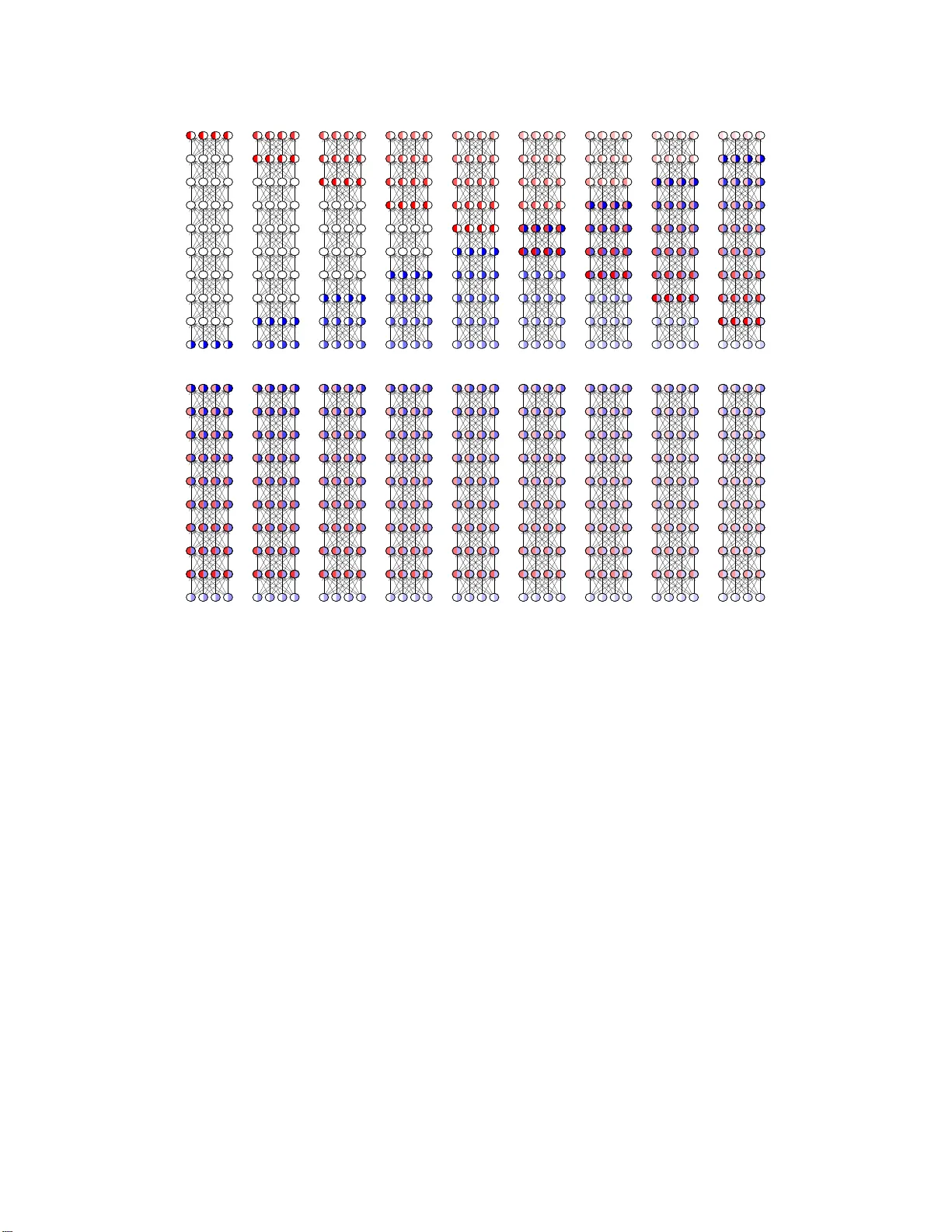
Backprop Diffusion is Biologi cally Plausible Alessandro Betti 1 , Marco Gori 1 , 2 1 DIISM, University of Siena, Siena, Italy 2 Maasai, Uni versitè Côte d’ A z ur, Nice, France {ales sandr o.bet ti2,marco.gori}@unisi.it Abstract The Back propa g ation algorithm relies on th e abstra c tio n o f using a n eural model that g ets rid of the notion of time, since the inpu t is m apped instanta n eously to the output. In this paper, we c laim that this abstraction of ignor ing tim e, along with the abrupt input chan ges that occur when feeding the training set, are in fact the reasons why , in som e p apers, Backp rop biological plausibility is r egarded as an arguable issue. W e show that as soon as a deep feedforward network operates with neuron s with time -delayed response, the b ackpro p weight upd ate turns out to be the ba sic equation of a biologically plausible diffusion process based on forward- backward waves. W e also show that such a proce ss very well appr oximates th e gradient fo r inpu ts that a r e not too fast with respect to the depth of the network. These rem a rks somewhat disclose the dif fusion process be h ind the backpro p equa- tion and leads us to in terpret the correspon ding alg orithm as a degener ation of a more gene r al dif fusion process that takes place also in neural networks with cyclic connectio ns. 1 Intr oduction Backprop agation enjoys t he pro perty of being an o ptimal algorithm for grad ient compu tation, which takes Θ( m ) in a feed forward network with m weigh ts [8, 9]. It is worth men tioning that the gra- dient compu tation with classic numerica l algorithm s would take O ( m 2 ) , which clear ly shows th e impressive advantage that is gained for now adays b ig network s. Howe ver , sin c e its co nception , Back- propag ation h as b e en the target of criticisms concernin g its biologic a l plausibility . Stefan Gro ssberg early pointed out the transport pr o blem that is inheren tly connected with the algorithm. Basically , for each neur o n, the delta error must be “tr a nsported ” for updating the weig hts. Hence, the algo- rithm re q uires each neuro n the availability of a precise knowledge of all of its d ownstream synapses. Related commen ts were given by F . Crick [6], who also poin ted ou t that backp rop seems to requ ire rapid circulatio n of the delta error bac k along axo ns from the synaptic outpu ts. I nterestingly enou gh, as discussed in the following, this is consistent with the ma in result of this paper . A nu mber o f studies hav e suggested solu tions to the weight transport p roblem . Recently , Lillicrap et al [11] ha ve suggested that random synap tic feedback weights can supp ort error back prop agation. However , any interpretatio n which neglects the role of time mig ht not fully capture the essence of biological plau- sibility . The intrigu ing marriage between energy-ba sed mod els with object function s fo r supervision that gives rise to Equilibrium Propag ation [12] is definitely better suited to capture the role o f time. Based the full trust on the role o f temporal ev olution, in [ 1], it is pointed ou t that, like other laws o f nature, learning can be formulated under th e framework of variational prin ciples. This paper spring s out from recent studies on the problem of learnin g visual features [3, 4, 2] and it was also stimulated by a nice analysis on the interp retation of Newtonian mechanics equations in the v ariational fram ework [10]. It is sho wn that when shifting f rom algorithms to laws of learning , one can clea r ly see the emergen ce o f the bio lo gical plausibility of Backpr op, an issue th at has been controversial since its spectacular impact. W e claim that the a lg orithm does r epresent a sor t o f d egen- Preprint. Under re vie w . t t + 1 t + 2 t + 3 t + 4 t + 5 t + 6 t + 7 t + 8 Figure 1: Fo rward and backward wav es on a t en-le vel network when the i nput and the supervision are kept con- stant. When selecting a certain frame—defined by the ti me inde x—the gradien t can consistently be computed by Backpropagation on “red-blue neurons”. eration of a natura l spatiote m poral dif fusion process that can clearly be und erstood when thinking of p erceptual tasks like speech and vision, whe r e signals p ossess smo o th pro p erties. In those tasks, instead of perfo rming the for ward-backward scheme for any fr ame, on e can p roper ly spr ead the weight up date acco rding to a diffusion scheme . While this is q uite an obviou s remark on p arallel computatio n, the disclosure of the degener ate d iffusion scheme behind Backprop , sheds light on its biological plausibility . The learning pr ocess th a t emerges in th is f ramework is based on co m plex diffusion wa ves that, howe ver , is dramatically simp lified un der the feedfo rward assumption, whe r e the propaga tio n is split into forward and bac k ward waves. 2 Backpr o p diffusion In th is section we consider m u ltilayered networks com posed o f L layers o f n eurons, but the results can easily be extend ed to any feedforward network characterized by an acyclic path of in terconn ec- tions. The layers ar e denoted by the index l , which ranges from l = 0 (input layer) to l = L (output layer). Let W l be the layer matrix and x t,l be the vector of th e neu r al output at layer l corr espondin g to discrete time t . Here we assume that the n etwork c a rries out a compu tation over time, so as, instead of regardin g the forward and backward steps as instantaneo u s proc e sses, we assume that the neuron al outp uts f ollow the time-d elay model: x t +1 ,l +1 = σ ( W l x t,l ) , (1) where σ ( · ) is th e neura l non -linear func tio n. In d oing so, when focussing on frame t the follo wing forward process takes place in a deep network o f L layers:            x t +1 , 1 = σ ( W 0 x t, 0 ) x t +2 , 2 = σ ( W 1 x t +1 , 1 ) = σ ( W 1 σ ( W 0 x t, 0 )) . . . x t + L,L = σ ( W L − 1 x t,L − 1 ) = . . . = σ ( W L − 1 σ ( W L − 2 . . . σ ( W 0 x t, 0 ) . . . )) . (2) Hence, the input x t, 0 is fo rwarded to lay ers 1 , 2 , . . . , L a time t + 1 , t + 2 , . . . , t + L , respec tiv ely , which can b e regard ed as a forward wa ve. W e can formally state that in put u t := x t, 0 is fo rwarded to layer κ by the operator κ → , that is κ → u t = x t + κ,κ . Likewise, when inspired by the backward step 2 (A) (B) t t + 1 t + 2 t + 3 t + 4 t + 5 t + 6 t + 7 t + 8 Figure 2: Forward and backward w av es on a ten-le vel network with slowly varying input and sup ervision. In (A) it is sho wn how t he i nput and backward signals fill the neurons; the wave fronts of the wav es are clearly vis- ible. Figure (B) instead sho ws the same dif fusion process in stationary conditions when the neurons are already filled up. In t his quasi-stationary condition the Backpropagation dif fusion algorithm very well approximates the gradient computation. In particular for l s = ( L + 1) / 2 = (9 + 1) / 2 = 5 there is a perfect backprop synchronization and the gradient is correctly computed. of Backpropa g ation, we can think of back-prop agating the delta error δ t,L on the output as follows:                    δ t +1 ,L − 1 = σ ′ L − 1 W T L − 1 δ t,L δ t +2 ,L − 2 = σ ′ L − 2 W T L − 2 δ t +1 ,L − 1 = ( σ ′ L − 2 W T L − 2 ) · ( σ ′ L − 1 W T L − 1 ) · δ t,L . . . δ t + L − 1 , 1 = σ ′ 1 W T 1 δ t + L − 2 , 2 = L − 1 Y κ =1 σ ′ κ W T κ · δ t,L Like for x t,l , we can fo rmally state that the output delta error δ t,L is propag ated back by the ope r- ator L − κ ← − d efined by δ t,L κ ← − := δ t + κ,L − κ . The following equ ation is still f ormally coming from Backprop agation, since it represen ts the classic factorization of forward an d ba c kward terms: g t,l = δ t,l · x t,l − 1 =  l − 1 − → u t − l +1  ·  δ t − L + l,L L − l ← −  (3) Clearly , g t,l is the result of a diffusion process that is characterized by the interaction of a for ward and of a backward wav e (see Fig. 1). Th is is a truly local spatiotemporal p rocess which is d efinitely biologically plausible. Notice th a t if L is odd the n for l s = ( L + 1) / 2 we hav e a perfect backp rop synchro n ization between th e inpu t and the sup ervision, since in this ca se the numb er of forward steps l − 1 eq uals the number of backward steps L − l . Clearly , the forward- backward wa ve synch r onization 3 t t + 1 t + 2 t + 3 t + 4 t + 5 t + 6 t + 7 t + 8 Figure 3: Forward and b a ckward wa ves on a ten- lev el network with r apidly ch anging sign al. In this case the Backp ropag ation diffusion equation does not properly appro ximate the gradient. How- ev er , also in this case, fo r l s = 5 we have per fect Backpr opagatio n synchronizatio n with correc t syncron iz a tion of the grad ient. Learning Mechanics Remarks ( W, x ) u W eights and neuronal outputs are interpreted as generalized coordi- nates. ( ˙ W , ˙ x ) ˙ u W eight variations and neuronal variations are interpreted as gener- alized velocities. A ( x, W ) S ( u ) The cog nitiv e action is the dual of the action in mechanics. T ab le 1: L in ks between learning theory and classical m echanics. takes place for L = 1 , which is a trivial case in which ther e is n o wa ve prop agation. The n ext case of per f ect synchr onization is fo r L = 3 . In this case, th e two hid den lay ers are in volved in one - step of f orward-bac kward p ropag ation. Notice tha t the per fect synchr onization com es with on e step delay in th e gradient com putation. In genera l, the comp u tation of the gradient in the lay er of perfect synch ronization is delayed of l s − 1 = ( L − 1) / 2 . For all other layer s, Eq. 3 tu r ns out to be a n ap prox imation of th e g radient computatio n, since the for ward and b ackward waves meet in layers of no perfect synch ronization . W e c a n pr omptly see that, as a matter of f act, synchro nization approx imatively holds when ev er u t is not too fast with respect to L (see Fig. 2 and 3). The maximum mismatch b e tween l − 1 and L − l is in fact L − 1 , so as if ∆ t is the quantization in terval required to perfor m th e compu tation over a layer, g ood synch ronization requires that u t is nearly con stant over intervals of length τ s = ( L − 1)∆ t . For example, a video stream , which is sampled at f v frames/sec requires to carry o ut the computation with time in te r vals bound ed by ∆ t = τ s / ( L − 1) = f v / ( L − 1) . 3 Lagrangian interpr etatio n of diffusion on graphs In the remainder of the p aper we show that the forward/back ward d iffusion of layered networks is just a special case of mor e gener al diffusion p rocesses that are at the basis of learnin g in neural networks characterized by graphs with any patter n of interconnectio ns. In p a rticular we show that this natu rally arises when f ormulatin g learn in g as a p a r simoniou s con straint satisfaction pro blem. W e use recent con n ections established b etween learn ing pr ocesses and laws of phy sics under the principle of least cognitive a c tio n [1]. In this p aper we make the a dditional assumptio n of defining conn e ctionist models of 1 2 3 4 5 learning in terms of a set of co nstraints that turn out to be sub sidiary condition s of a variational pr oblem [7]. Let us co nsider the classic example of the feedforward network used to comp ute the XOR predicate. If we deno te with x i the o utputs of e a ch n euron and with w ij the weigh associated with the arch i − − − j , th en for the n eural n e twork in the fig u re we have x 3 = σ ( w 31 x 1 + w 32 x 2 ) , x 4 = 4 σ ( w 41 x 1 + w 42 x 2 ) and x 5 = σ ( w 53 x 3 + w 54 x 4 ) . Therefo re in the w − x space th is composition al relations b etween the nodes variables can be regard ed as co nstraints, namely G 3 = G 4 = G 5 = 0 , where: G 3 = x 3 − σ ( w 31 x 1 + w 32 x 2 ) , G 4 = x 4 − σ ( w 41 x 1 + w 42 x 2 ) , G 5 = x 5 − σ ( w 53 x 3 + w 54 x 4 ) . In addition to these constraints we ca n also regard the way with which we assign the inpu t values a s additional co nstraints. Suppose we want to compute the v alue of th e network on the input x 1 = e 1 and x 2 = e 2 , wh ere e 1 and e 2 are two scalar values; this two assignments can be regarded as two additional con straints G 1 = G 2 = 0 where G 1 = x 1 − e 1 , G 2 = x 2 − e 2 . First of all let us describe the architecture of the models that we will address. Giv en a simple digraph D = ( V , A ) of order ν , without loss of gener ality , we can assume V = { 1 , 2 , . . . , ν } and A ⊂ V × V . A neur a l network co nstructed o n D co n sists of a set of maps i ∈ V 7→ x i ∈ R and ( i, j ) ∈ A 7→ w ij ∈ R together with ν co nstraints G j ( x, W ) = 0 j = 1 , 2 , . . . ν wher e ( W ) ij = w ij . L et M ν ( R ) be the set of all ν × ν real matr ices and M ↓ ν ( R ) th e set of all ν × ν strictly lower triangular m atrices over R . If W ∈ M ↓ ν ( R ) we say that the NN has a feed forward structur e. In this pap er w e will consider b oth feedfor ward NN and NN with cycles. The r elations G j = 0 for j = 1 , . . . , ν spec if y the co mputation al sch e m e with wh ich the inf ormation d iffuses tr ough the n etwork. In a typical network with ω inpu ts these constrain ts are defined as f o llows: For any vector ξ ∈ R ν , fo r any matrix M ∈ M ν ( R ) with entries m ij and for any giv en C 1 map e : (0 , + ∞ ) → R ω we defin e the constraint on neuron j when the example e ( τ ) is pre sented to the network as G j ( τ , ξ , M ) :=  ξ j − e j ( τ ) , if 1 ≤ j ≤ ω ; ξ j − σ ( m j k ξ k ) if ω < j ≤ ν , (4) where σ : R → R is of class C 2 ( R ) . Notice that the dependence of th e constraints on τ reflects the fact th at the computatio ns of a neur al n etwork should b e based on external inputs. Principle of Least Cognitive Action Like in the case o f classical mechan ics, when dealing with learning p rocesses, we are interested in the tempo ral dyn a mics of the variables exposed to the data from which the learnin g is sup posed to happen . Depending on the structure of the matrix M , it is u seful to distingu ish between feedfor ward n etworks and n etworks with loops (recur rent neural networks). Let us therefor e consid e r the function al A ( x, W ) := Z 1 2 ( m x | ˙ x ( t ) | 2 + m W | ˙ W ( t ) | 2 )  ( t ) dt + F ( x, W ) , (5) with F ( x, W ) := R F ( t, x, ˙ x, ¨ x, W, ˙ W , ¨ W ) dt and t 7→  ( t ) a p ositiv e co n tinuou sly differentiable function , subject to the constrain ts G j ( t, x ( t ) , W ( t )) = 0 , 1 ≤ j ≤ ν, (6) where the map G ( · , · , · ) is taken as in Eq. (4). Let ( G ξ G M ) be th e Jacobian matrix of the constrain ts G with respect to x and W , where it is inten d ed th at the first ν rows contain the gradien ts of G with respect to its second argument:  G ξ G M  ij ≡ G j ξ i , for 1 ≤ i ≤ ν . V ariational pro blems with subsidiar y con ditions can be tackled u sin g the method of Lagran g e multi- pliers to convert the constrained pr o blem in to an unconstrain ed one [ 7]). In order to use this method it is necessary to verify an in depend ence hyp othesis between the co n straints; in this case we need to check that the matrix ( G ξ G M ) is full rank. Inter estingly , the follo wing pr o position holds true: Proposition 1. The ma trix ( G ξ G M ) ∈ M ( ν 2 + ν ) × ν ( R ) is full rank. Pr oo f. First of all notice that if ( G ξ ) ij = G j ξ i is full rank also ( G ξ G M ) has this property . Then, since G j ξ i ( τ , ξ , M ) =  δ ij , if 1 ≤ j ≤ ω ; δ ij − σ ′ ( m j k ξ k ) m j i if ω < j ≤ ν , 5 we immediately notice that G i ξ i = 1 an d that for all i > j we have G i ξ i = 0 . This means that ( G j ξ i ( τ , ξ , M )) =     1 ∗ · · · ∗ 0 1 · · · ∗ . . . . . . . . . . . . 0 0 · · · 1     , which is clearly full rank. Notice tha t th is r esult heavily d epends on the assumption W ∈ M ↓ ν ( R ) ( triangula r matr ix ), wh ich correspo n ds to feedfo rward arch itectures. Derivation of the Lagrangian multipliers—feedforward networks F ollowing the spirit o f the principle of least cog nitive action [1], we begin by d eriving the constrained E u ler-Lagrange (EL) equations associated with the functional ( 5) unde r subsidiar y c ondition s (6) that refer to feedforward neural networks. The constrained function a l is A ∗ ( x, W ) = Z 1 2 ( m x | ˙ x ( t ) | 2 + m W | ˙ W ( t ) | 2 )  ( t ) − λ j ( t ) G j ( t, x ( t ) , W ( t )) dt + F ( x, W ) , (7) and its EL-equation s thus read − m x  ( t ) ¨ x ( t ) − m x ˙  ( t ) ˙ x ( t ) − λ j ( t ) G j ξ ( x ( t ) , W ( t )) + L x F ( x ( t ) , W ( t )) = 0; (8) − m W  ( t ) ¨ W ( t ) − m W ˙  ( t ) ˙ W ( t ) − λ j ( t ) G j M ( x ( t ) , W ( t )) + L W F ( x ( t ) , W ( t )) = 0 , (9) where L x F = F x − d ( F ˙ x ) /dt + d 2 ( F ¨ x ) /dt 2 , L W F = F W − d ( F ˙ W ) /dt + d 2 ( F ¨ W ) /dt 2 are the function al deriv ati ves of F with respect to x and W respectively (see [ 5]). An expression for the Lagra nge multipliers is deri ved by differentiating two times the equations of th e architectural co nstraints with respect to the time an d using the obtain ed expression to su b stitute the second ord er ter ms in the Euler equation s, so as we get:  G i ξ a G j ξ a m x + G i m ab G j m ab m W  λ j =   G i τ τ + 2( G i τ ξ a ˙ x a + G i τ m ab ˙ w ab + G i ξ a m bc ˙ x a ˙ w bc ) + G i ξ a ξ b ˙ x a ˙ x b + G i m ab m cd ˙ w ab ˙ w cd  − ˙  ( ˙ x a G i ξ a + ˙ w ab G i m ab ) + L x a F G i ξ a m x + L w ab F G i m ab m W , (10) where G i τ , G i τ τ , G i ξ a , G i ξ a ξ b , G i m ab and G i m ab m cd are the gradients and the hessians of con straint (6). Suppose n ow th at we want to solve Eq. (8)–(9) w ith Cauchy in itial co nditions. Of course we must choose W (0) and x (0) such that g i (0) ≡ 0 , where we posed g i ( t ) := G i ( t, x ( t ) , W ( t )) , fo r i = 1 , . . . , ν . Howev er since the constraint m u st h old also for all t ≥ 0 we must also have at least g ′ i (0) = 0 . T hese conditions written explicitly mean s G i τ (0 , x (0) , W (0)) + G i ξ a (0 , x (0) , W (0)) ˙ x a (0) + G i m ab (0 , x (0) , W (0)) ˙ w ab (0) = 0 . If the con straints does not depen d explicitly on time it is sufficient to to choose ˙ x (0) = 0 and ˙ W (0) = 0 , w h ile for time dependent constraint th is co ndition lea ves G i τ (0 , x (0) , W (0)) = 0 , which is an ad ditional con straint on the initial co ndition s x (0) and W (0) to be satisfied. Therefo re one possible consistent w ay to impose Cauchy conditions is G i (0 , x (0) , W (0)) = 0 , i = 1 , . . . , ν ; G i τ (0 , x (0) , W (0)) = 0 , i = 1 , . . . , ν ; ˙ x (0) = 0; ˙ W (0) = 0 . (11) 6 Reduction to Backpropagatio n T o unde r stand th e behaviour of the Eu ler equ ations (8) and (9) we observe that in the case of feedforward networks, as it is w e ll known, th e con straints G j ( t, x, W ) = 0 can be solved for x so that eventually we can express the v alue of the ou tput n euron s in terms of the value of the inp ut neurons. If we let f i W ( e ( t )) be the value of x ν − i when x 1 = e 1 ( t ) , . . . , x ω = e ω ( t ) , then the theory d e fined by ( 5) under sub sidiary cond itions (6) is equivalent, wh en m x = 0 and  ( t ) = exp( ϑt ) , to the unco nstrained theo ry defined by Z e ϑt  m W 2 | ˙ W | 2 − V ( t, W ( t ))  dt (12) where V is a loss fu nction fo r which a po ssible ch oice is V ( t, W ( t )) := 1 2 P η i =1 ( y i ( t ) − f i W ( E ( t ))) 2 with y ( t ) an assigned target. The Euler equations associated with (1 2) are ¨ W ( t ) + ϑ ˙ W ( t ) = − 1 m W V W ( t, W ( t )) , (13) that in the limit ϑ → ∞ and ϑm → γ reduce s to the gra dient me th od ˙ W ( t ) = − 1 γ V W ( t, W ( t )) , (14) with learning rate 1 /γ . Notice that the pr esence of th e term  ( t ) that we prop o sed in the gen- eral theor y it is e ssential in ord er to h av e a lea r ning b ehaviour as it respon sib le of the dissipative behaviour . T yp ically the term V W ( t, W ( t )) in Eq. (14) can be e v aluated using the Backp ropag ation algorithm; we will now show th at Eq. ( 8)–(10) in the lim it m x → 0 , m W → 0 , m x /m W → 0 repr o duces Eq. (14) where the term V W ( t, W ( t )) explicitly assumes the form prescribed by BP . In order to see this choose ϑ = γ /m W ,  ( t ) = exp( ϑt ) , F ( t, x ( t ) , ˙ x ( t ) , ¨ x ( t ) , W ( t ) , ˙ W ( t ) , ¨ W ( t )) = − e ϑt V ( t, x ( t )) , and multiply b oth sides of Eq. ( 8)–(10) by exp( − ϑt ) ; then take the limit m x → 0 , m W → 0 , m x /m W → 0 . In this limit Eq. (9) and Eq. (10) becomes re sp ectiv ely ˙ W ij = − 1 γ σ ′ ( w ik x k ) δ i x j ; (15) G i ξ a G j ξ a δ j = − V x a G i ξ a , (16) where δ j is the limit of exp( − ϑt ) λ j . Because the matrix G i ξ a is in vertible Eq. (16) yields T δ = − V x , (17) where T ij := G j ξ i . T his matrix is an upper triangular matr ix thus showing e xplicitly th e backward structure of the p ropag a tion of the delta error of the Backp ropag ation alg orithm. In deed in Eq. (15) the Lagrange multiplier δ plays the ro le of the delta er ror . In order to better u n derstand the perfec t red uction of our app r oach to the backpro p alg orithm con- sider the following example. W e simp ly con sider a feedf orward network with an input, an output and an hidden neuron. In this case the matrix T is T =   1 − σ ′ ( w 21 x 1 ) w 21 0 0 1 − σ ′ ( w 32 x 2 ) w 32 0 0 1   . Then acco r ding to Eq. (17) the L a grange multip liers are derived as f ollows δ 3 = − V x 3 , δ 2 = σ ′ ( w 32 x 2 ) w 32 δ 3 , and δ 1 = σ ′ ( w 21 x 1 ) w 21 δ 2 . This is exactly the Backpro pagation form ulas for the delta e rror . Notice th at in th is theory we also ha ve an e xpression for th e multipliers of the inpu t neuron s, even tho ugh, in th is case, they ar e not used to u pdate the weights (see Eq. (1 5)). Diffusion on cyclic g raphs The co nstraint-based analysis car ried out so far assumes holo nomic constraints, whereas th e claim of this pap er is that we canno t neglect temporal dependencies, which leads to expressing neural models by non -holon omic constrain ts. In doin g so, we go beyond the constraints expressed by Eq. (6) wh ich imply a n infinite velocity of diffusion o f information. Since 7 we are stressing the imp o rtance of time in learning processes, it is natur al to assume th a t the velocity of inform a tion diffusion throug h a network is finite. In the discrete setting of com putation this is reflected by the mo del 1 d iscussed in Section 2. A simple classic tran slation of this constrain t in continuo us time is c − 1 ˙ x i ( t ) = − x i ( t ) + σ ( w ik ( t ) x k ( t )) , (18) where c > 0 can b e inter preted as a “diffusion sp e ed”. In station ary situation inde e d Eq. (1 8) coincide with the usua l neur on equation in Eq. (6). Howe ver , we are in fro n t of a muc h mo re complicated co nstraint, since not only it inv olves th e variables x and w , but also th e ir d eriv ati ves. Such con straints are called non -holo nomic co n straints. Now we snow show ho w to determine the stationarity conditions of the functional 1 A ( x, W ) = Z  m x 2 | ˙ x ( t ) | 2 + m W 2 | ˙ W ( t ) | 2 + F ( t, x, W )   ( t ) dt under the nonholo mic constraints G i ( t, x ( t ) , W ( t ) , ˙ x ( t )) := c − 1 ˙ x i ( t ) + x i ( t ) − σ ( w ik ( t ) x k ( t )) = 0 , i = 1 , . . . , r, (19) by making use of the rule of the Lagrange m u ltipliers. As usual we co n sider the stationary points of the functional A ∗ ( x, W ) = Z  m x 2 | ˙ x ( t ) | 2 + m W 2 | ˙ W ( t ) | 2 + F ( t, x, W )   ( t ) dt − Z λ j ( t ) G j ( t, x ( t ) , W ( t ) , ˙ x ( t )) dt. The Euler equations for A ∗ are c − 1 ˙ x i ( t ) + x i ( t ) − σ ( w ik ( t ) x k ( t )) = 0; − m W  ( t ) ¨ W ( t ) − m W ˙  ˙ W ( t ) − λ j G j M ( t, x ( t ) , W ( t ) , ˙ x ( t )) +  ( t ) F W ( t, x ( t ) , W ( t )) = 0; − m x  ( t ) ¨ x ( t ) − m x ˙  ˙ x ( t ) + ˙ λ j G j p ( t, x ( t ) , W ( t ) , ˙ x ( t )) + λ j d dt G j p ( t, x ( t ) , W ( t ) , ˙ x ( t )) − λ j G j ξ ( t, x ( t ) , W ( t ) , ˙ x ( t )) +  ( t ) F x ( t, x ( t ) , W ( t )) = 0 . Again, if we assume that F ( t, x, W ) = − V ( t, x ) ,  ( t ) = e ϑt , δ j = e − ϑt λ j and w e explicitly use the expression f or G j p we get c − 1 ˙ x i ( t ) + x i ( t ) − σ ( w ik ( t ) x k ( t )) = 0; − m W ¨ W ( t ) − m W ϑ ˙ W ( t ) − δ j G j M ( t, x ( t ) , W ( t ) , ˙ x ( t )) = 0; − m x ¨ x ( t ) − m x ϑ ˙ x ( t ) + c − 1 ˙ δ − δ j G j ξ ( t, x ( t ) , W ( t ) , ˙ x ( t )) − V ξ ( t, x ( t )) = 0 . This systems of equ ations can be better interpreted in the limit in which we recovered the backprop rule in Section 4; that is to say in th e limit m x → 0 , m x → 0 and m x /m W → 0 , θ → ∞ and θm W = γ fixed. Under this condition s, we have the following fu rther reduction c − 1 ˙ x i ( t ) + x i ( t ) − σ ( w ik ( t ) x k ( t )) = 0; ˙ W ( t ) = − 1 γ δ j ( t ) G j M ( t, x ( t ) , W ( t ) , ˙ x ( t )); c − 1 ˙ δ ( t ) = δ j ( t ) G j ξ ( t, x ( t ) , W ( t ) , ˙ x ( t )) + V ξ ( t, x ( t )) . (20) The equation that defines the Lagr a n ge multipliers δ is now a differential equa tio n that explicitly giv es us the c o rrect updatin g rule in stead of a instantaneous equation that must be solved for each t . As the dif fusion speed becom es infinite ( c → + ∞ ) Eq. (20) reprodu ce Backpro pagation , which is consistent with the intuiti ve explan ation tha t arises from Fig. 1, 2, 3. 1 Notice that here we are ov erloading the symbol F since in this section we assume that the L agrangian F depends only on t , x and W . 8 4 Conclusions In this paper we h ave shown that th e lo ngstandin g debate on the biological plau sib ility of Backp rop- agation can simply be add ressed by d istinguishing the for ward - backward local diffusion p rocess for weight up dating with re spect to the alg orithmic gradien t compu tation over all the n et, which requires the tr ansport o f the delta error throu gh the entire g r aph. Basically , the algorithm expresses the degeneratio n of a biolo gically plausible diffusion pro cess, which comes from the assumption of a static neur al model. The main conc lusion is that, more than Backpro pation, the appropr iate target of the mentioned lo ngstandin g biological plausibility issues is the assumptio n of an instantan eous map from the input to the output. The forward-b ackward w av e propag ation behind Backprop aga- tion, which is in fact at the basis o f the co rrespon ding algo rithm, is p r oven to be lo cal and d efinitely biologically p lausible. This paper has sh own tha t an opp ortun e em beddin g in time of deep networks leads to a natur al in ter pretation of Backprop as a diffusion p rocess which is fully local in space and time. The giv en analysis on any graph-based neur al architectu res sugg ests that spatiotemp oral diffu- sion takes place according to the interactions of forward and backward waves, which arise fro m the en vironmen tal interaction. While th e f orward wa ve is gener ated by the inp ut, the b ackward wave arises from th e output; the special way in which they interact for classic feedforward network corre- sponds to the degeneration of this dif fusion process which takes place at infinite velocity . Howe ver , apart from this theoretical limit, Back propa gation diffusion is a tru ly local process. Br oader Impact Our work is a foundatio nal study . W e b eliev e that there are neither ethical aspects no r futu re societal consequen ces that should be discussed. Refer ences [1] Alessandro Betti and Marco Gori. T he principle of least cognitiv e action. Theor . Comput. Sci. , 633:83 –99, 20 16. [2] Alessandro Betti a nd Marc o Gori. Conv o lutional n etworks in visual environments. CoRR , abs/1801 .0711 0, 20 18. [3] Alessandro Betti, Mar c o Gori, and Stefano Melacci. Cognitive action laws: T h e case of visual features. IEEE transactions on neural networks and learning systems , 2019. [4] Alessandro Betti, M arco Gori, and Stefano Melacci. Motion inv ariance in visual environments. In Pr oceeding s of the T wenty-Eighth I nternation al Joint Conference on Artificial Intelligence, IJCAI-19 , pages 20 09–20 15. Internatio nal Joint Con ference s on Artificial Intelligence Organi- zation, 7 2019. [5] R Couran t and D Hilbert. Meth ods of Mathematical Physics , volume 1, pag e 190. Interscience Publ., Ne w Y or k and London, 19 62. [6] Francis Crick. The recent excitement abo ut neural networks. Nature , 33 7:129 –132 , 1 989. [7] M. Giaquinta and S. Hildebrand. Calcu lus of V ariation s I , volume 1. Spring er, 1 996. [8] Ian Goodfellow , Y oshua Bengio, and Aa r on Courville. Deep Learning . Th e MIT Press, 2016. [9] Marco Gori. Machine Learning: A Constrained-Based Ap pr o ach . Morgan Kauffman, 2018 . [10] Matthias L ier o and Ulisse Stefanelli. A new min imum princip le for lag rangian mec h anics. Journal of Nonlinea r Science , 2 3:179 – 204, 201 3 . [11] T .P . Lillicrap , D. Cownden, D.B. T wed, and C.J. Akerm a n. Random synap tic f e e dback weights support error backpro p agation for deep learning. Natur e Communications , Jan 2 016. [12] Benjamin Scellier and Y oshua Beng io. Equivalence of equilibrium pro pagation and rec u rrent backpr o pagation . Neural Computation , 31(2), 2 019. 9