Predicting Motion of Vulnerable Road Users using High-Definition Maps and Efficient ConvNets
Following detection and tracking of traffic actors, prediction of their future motion is the next critical component of a self-driving vehicle (SDV) technology, allowing the SDV to operate safely and efficiently in its environment. This is particular…
Authors: Fang-Chieh Chou, Tsung-Han Lin, Henggang Cui
Pr edicting Motion of V ulnerable Road Users using High-Definition Maps and Efficient Con vNets Fang-Chieh Chou, Tsung-Han Lin, Henggang Cui, Vladan Radosa vlje vic, Thi Nguyen, Tzu-Kuo Huang, Matthew Niedoba, Jeff Schneider and Nemanja Djuric 1 Abstract — Follo wing detection and tracking of traffic actors, prediction of their future motion is the next critical component of a self-driving vehicle (SD V) technology , allowing the SD V to operate safely and efficiently in its en vironment. This is particularly important when it comes to vulnerable road users (VR Us), such as pedestrians and bicyclists. These actors need to be handled with special care due to an increased risk of injury , as well as the fact that their behavior is less predictable than that of motorized actors. T o address this issue, in the curr ent study we present a deep learning-based method f or predicting VR U movement, where we rasterize high-definition maps and actor’ s surroundings into a bird’ s-eye view image used as an input to deep convolutional networks. In addition, we propose a fast architecture suitable for real-time inference, and perform an ablation study of various rasterization approaches to find the optimal choice for accurate prediction. The results strongly indicate benefits of using the proposed approach for motion prediction of VR Us, both in terms of accuracy and latency . I . I N T RO D U C T I O N Predicting mo vement of traf fic actors is a critical part of the autonomous technology . Once a self-driving vehicle (SD V) successfully detects and tracks a traffic actor in its vicinity , it needs to understand how will they mov e in the near future in order for both actors and SD V to be safe during operations [1]. This holds particularly true for vulnerable road users (VRUs), defined as traffic actors with increased risk of injury , unprotected by an outside shield [2]. Road planners and policy makers hav e recognized this problem many decades ago, and attempted to mitigate it through sev eral means. This included leg al frame works, designing new road types (e.g., segre gating VR Us from motorized actors), educating both driv ers and VR Us (with particular focus on children and elderly that are at an even greater risk than others [2], [3]), to name a fe w . These approaches hav e howe ver given limited results, and in the US proportion of VR U deaths within overall traf fic fatalities has actually increased between 2008 and 2017 from 14% to 19% [4] despite these best efforts. In the current study we address a critical aspect of the SD V technology , focusing on predicting future motion for VR Us, namely pedestrians and bicyclists. The main contributions of the paper are summarized below: • W e present a system for motion prediction of VR U traffic actors, building upon recently proposed context rasterization techniques [1]; 1 Authors are with Uber Adv anced T echnologies Group, located at 3011 Smallman Street, Pittsburgh, P A, USA. Corresponding author e-mail: ndjuric@uber.com • W e propose a f ast and ef ficient con volutional neural network (CNN) architecture, suitable for running real- time onboard an SD V operating in crowded urban scenes with a large number of VR U actors; • W e present a detailed study of various rasterization settings identifying the optimal settings for accurate prediction, and provide critical insights into which parts of the system contribute the most to the accuracy; • Follo wing completion of offline tests the system was successfully tested onboard SDVs. I I . R E L A T E D W O R K Efficient and accurate motion prediction of VR Us is one of the ke y requirements to safely deploy SD Vs in complex urban en vironments [5]. In this section we pro vide a literature ov ervie w of motion prediction of pedestrians and bicyclists in the context of autonomous driving. Motion pr ediction. A common approach for prediction of VR U mov ement in autonomous driving systems is to use motion model from a tracking component to predict their future states. Tracking modules of most existing autonomous systems use either the Bro wnian or the constant velocity motion models [6]. These models do not take into account scene contexts, and therefore fail in long-term prediction tasks as VRU motion follows comple x patterns constrained by static and dynamic obstacles along the path. T raditionally , hand-crafted features were used for motion prediction of VR Us with respect to their surroundings. The social force model for pedestrian motion prediction incorporated inter - activ e forces that guide pedestrians towards their goals and enforce collision av oidance among pedestrians, as well as between pedestrians and static obstacles [7], [8]. Similar approach was applied for bicyclist motion prediction [9]. In [10] authors introduced a motion model for bicyclist motion prediction that incorporates knowledge of the road topology . The authors were able to improve prediction accuracy by using specific motion models for a pre-specified set of canonical directions. In [11] interacting Gaussian Processes (GPs) with multiple goals were applied to model human cooperation in dense crowds for robot navigation. Authors of [12] predicted pedestrian trajectories by incorporating semantic scene features into the GP model, such as relativ e distance to curbside and state of traffic lights. A significant number of studies are dev oted to modeling pedestrian motion using maximum entropy In verse Reinforcement Learning (IRL) [13]. In a followup work [14] the authors introduced an IRL model based on a set of manually designed feature functions that capture interaction and collision a voidance behavior of pedestrians. While the approaches are capable of predicting pedestrian and bicyclist motions in many sce- narios, the need for manual design of features makes them hard to scale in complex driving en vironments [15]. Motion prediction using deep learning. Inspired by their success in various areas of computer vision and robotics, many deep learning-based approaches were recently pro- posed for the motion prediction task in order to model object-object and object-scene interactions which may not be straightforward to represent manually . Most of deep learning approaches are based on Long Short-T erm Memory (LSTM) variant of recurrent neural networks (RNNs) [16]. Authors of [17] used a sequence-to-sequence LSTM encoder-decoder architecture to predict pedestrian position and heading. Incor - porating angular information in addition to temporal features led to a significant improvement in accuracy . W ith respect to modeling of dynamic context, [18] proposed an LSTM- based approach for pedestrian motion prediction employing a “social pooling” layer that uses spatial information of nearby actors to implicitly model interactions among them. V emula et al. [19] proposed “social attention” method to predict motion by estimating relative importance of pedes- trians through an attention layer . Recently , [20] proposed an LSTM-based Generativ e Adversarial Network (GAN) to generate and predict socially feasible motions. On the other hand, with respect to modeling of static context [21] proposed an LSTM-based model that incorporates the map of static obstacles and position of surrounding pedestrians. Moreov er , [22] presented SoPhie, an LSTM-based GAN system for predicting physically and socially acceptable pedestrian trajectories using an RGB image from the scene and the trajectory information of surrounding actors. Simi- larly , in recent work [15], [23] authors incorporated scene information as well as human movement trajectories. In addition to LSTM-based methods, [24] proposed CNN-based approach where conv olutional layers are utilized to handle temporal dependencies. [25] used an interaction-aware tem- poral CNN to predict pedestrian trajectories. [26] proposed a hybrid LSTM-CNN model that encodes actor states with LSTM and uses CNN to extract actor interaction features, while taking the varying behaviors of different road actors into account. [27] use CNNs for joint detection, tracking, and prediction. Howe ver , these models do not consider scene context, which can provide a strong signal on how the actors would move. On the other hand, in [28] the authors included map info to also predict high-le vel intent of vehicles, unlike our model that focuses on VR U actors instead. Efficient CNN architectur es. Since the introduction of seminal AlexNet [29], researchers made significant progress in improving CNNs to make them more accurate and effi- cient. The state-of-the-art architectures, such as VGG [30] or ResNet [31], tend to have a large number of layers running expensi ve computations, making them unsuitable for real- time inference. Recent proposals such as MobileNet [32] and Shuf fleNet [33] replaced regular con v olutional operator with a more efficient depthwise separable or group con v olu- Fig. 1: Example input raster for a pedestrian model with ov erlaid ground-truth (green) and output trajectory (blue); the target actor is colored in red and placed at the bottom- center of the raster image (indicated by the red arro w) tions, making them small and fast for mobile applications. MobileNet-v2 (MNv2) [34] further improved the original MobileNet by combining depthwise con volution with resid- ual connections and bottleneck layers proposed in ResNet. One problem of this work is its focus on reducing number of floating point operations per second (FLOPS) instead of optimizing for actual latency on de vices. More recently , MnasNet [35] applied search algorithms [36] to optimize MNv2 architecture for both accuracy and inference latency on mobile devices, and is able to improv e both while main- taining similar FLOPS. Shuf fleNet v2 [37] proposed se v- eral guidelines for designing fast networks beyond counting FLOPS, and applied these guidelines to design architectures suitable for both GPUs and mobile CPUs. In this paper we build upon and extend the MNv2 model, improving its speed on GPUs without compromising prediction accurac y . I I I . P RO P O S E D A P P R OAC H W e build upon work described in [1], which considered vehicle actors and used rasterized images of actor context as an input to CNNs to predict future trajectories. In this study we extend the methodology to VR U actors (see Figure 1 for an example of pedestrian motion prediction). Importantly , we improv e the existing method’ s accuracy and inference speed by e xploring two critical aspects. First, we e xperiment with different variations of the CNN architectures, and propose a nov el architecture that significantly reduces inference latency without af fecting accuracy; this is necessary to achiev e real-time inference onboard an SD V in crowded urban en vironments comprising lar ge number of VRUs. Second, we explore dif ferent rasterization configurations to find an optimal setup for highly accurate predictions of VRU actors. Let us assume we have access to real-time data streams coming from sensors such as lidar, radar , or camera, installed aboard an SD V . In addition, assume these inputs are used by an existing detection and tracking system, outputting state estimates S for all surrounding actors (state comprises the bounding box, position, velocity , acceleration, heading, and heading change rate). Denote a set of discrete times at which tracker outputs state estimates as T = { t 1 , t 2 , . . . , t T } , where Inputs Conv 1 × 1, BN, ReLU DwConv 3× 3, BN, ReLU Conv 1 × 1, BN Add H×W×C H×W× k C H×W× k C H×W×C Inputs Conv 1 × 1, ReLU Conv 1 ×1 DwConv 3× 3, Bias Add H×W×C H×W× k C H×W×C H×W×C Inputs Conv 1 × 1, ReLU Conv 1 ×1 DwConv 3× 3, stride=2, Bias Add H×W×C in H×W× k C in H×W×C out H/2 × W/2 ×C out Dw Conv 3× 3, stride=2 Conv 1 ×1 (a) Regular block of MNv2 (b) Regular block of FMNet (c) Stride=2 block of FMNet Fig. 2: Building blocks of MobileNet-v2 [34] and the proposed FastMobileNet (FMNet) architecture time gap between consecuti ve time steps is constant (e.g., the gap is equal to 0 . 1 s for tracker running at a frequency of 10 H z ). Then, we denote state output of a tracker for the i -th actor at time t j as s i j , where i = 1 , . . . , N j with N j being a number of unique actors tracked at t j . Moreover , we assume access to a detailed, high-definition map M of the SDV’ s operating area, including road and crosswalk locations, lane directions, and other relev ant map information. Using the state estimates and high-definition map, for each actor of interest we rasterize an actor-specific bird’ s-eye view raster image encoding the actor’ s surrounding map and traffic actors, as illustrated in Figure 1. Then, giv en the i -th actor’ s raster image at time step t j and state estimate s i j , we use a CNN model to predict a sequence of its future states up to the prediction horizon of H time steps [ s i ( j + 1 ) , . . . , s i ( j + H ) ] (see model architecture in Figure 3a), trained to minimize the av erage displacement error (ADE) of the predicted trajectory points. W ithout loss of generality , in this work we simplify the task to infer the i -th actor’ s future x - and y -positions instead of full state estimates, while the remaining states can be deriv ed from the current state s i j and the future predicted position estimates. Both past and future positions at time t j are represented in the actor-centric coordinate system deri ved from actor’ s state at time t j , where forward direction is x - axis, left-hand direction is y -axis, and actor’ s bounding box centroid represents the origin. Follo wing the approach in [1] we use an MNv2 model as the base CNN to compute future positions from the input raster image. Belo w we describe improvements to this architecture, followed by discussion of v ariations to the rasterization process that were considered in the study . A. Impr oved CNN arc hitecture for fast inference 1) Base CNN: In this section we propose se veral mod- ifications to the MNv2 architecture that lead to significant speedup of GPU inference, making it feasible to perform real-time inference when our SD Vs operate in urban scenes containing large number of VR Us. MNv2 is based on the in verted bottleneck block illustrated in Figure 2a. In each block, the input feature map is first upsampled to k times more channels with 1 × 1 conv olutions ( k is set to 6 in the original MNv2), followed by 3 × 3 depthwise con volution (DwCon v) applied to the upsampled feature map. Then, the feature map is compressed back to the original channel size using 1 × 1 con volution, and summed with the initial input through residual connection. Non-linear activ ation function (e.g., ReLU) is applied only in the upsampled phase, as non- linearity in the bottlenecked phase (before the upsampling or after the compression) causes too much information loss and hurts model performance. BatchNorm (BN) is used in all three layers. While the majority of the FLOPS are in the 1 × 1 conv olutions (amounting to 87% of the total), the other operations still incur non-negligible cost. As discussed in [37], FLOPS itself is not an accurate metric of latency , and another important factor is the number of memory access operations (MA C). Operations such as DwCon v , BatchNorm, ReLU, and BiasAdd, while having small FLOPS, typically incur heavy MAC. This especially holds true for MNv2, where operations in the upsampled phase have k times more MA C than the same operations in the bottlenecked phase. Compared to MNv2, in the proposed novel CNN archi- tecture called FastMobileNet (FMNet) we move most of the operations originally in the upsampled phase into the bottlenecked phase, reducing their FLOPS and MA C by a factor of k , as illustrated in Figure 2b . Note that we show the architecture for an equal number of input and output channels, if they are not the same an additional 1 × 1 con volution is applied after the residual connection. The only remaining operation in the upsampled phase is a ReLU. Similarly to MNv2, no ReLU is applied in the bottlenecked phase since applying non-linearity there causes significant information loss. The layers are linear in the bottlenecked phase, and we only apply one BiasAdd at the end of the block as applying multiple BiasAdd in consecuti ve linear layers does not increase model expressi veness. W e do not use BatchNorm in FMNet as we found that the model conv er ges well without it, and excessiv e BatchNorms cost additional computation time. In addition, we need to allo w different strides in order to reduce height and width of the feature map during feature extraction. The FMNet block supporting this operation is similar to the regular block (see Figure 2c), except the original input is do wnsampled to the correct output size for residual connection. The base model (further discussed and extended in the follo wing section) is illustrated in Figure 3a, and the FMNet architecture corresponding to the CNN part is sho wn in T able I, where the layer sizes and T ABLE I: Architecture of FastMobileNet (upsample factor for all FMNet blocks is set to k = 6) Layer Output size Stride Repeats Raster image 300 × 300 × 3 − − Con v 3 × 3 150 × 150 × 24 2 1 DwCon v 3 × 3 75 × 75 × 24 2 1 FMNet block 1 75 × 75 × 12 1 2 FMNet block 2 38 × 38 × 16 2 3 FMNet block 3 19 × 19 × 32 2 4 FMNet block 4 19 × 19 × 48 1 3 FMNet block 5 10 × 10 × 80 2 3 FMNet block 6 10 × 10 × 160 1 1 Con v 1 × 1 10 × 10 × 640 1 1 Global average pooling 1 × 1 × 640 1 1 Raster input FC State input Base CNN Flatten Raster feature State input Concat FC 1×4096 Output 300×300×3 (a) (b) Raster input State input CNN part 1 CNN part 2 FC, Reshape Conv 1×1 19×19×32 Add FC Output 19×19×3 300×300×3 19×19×32 FastMobileNet Fig. 3: Feature fusion through (a) concatenation; and (b) spatial fusion block repeats of the model are based on MNv2-0.5 [34] (i.e., MNv2 with halved channel sizes in all layers). 2) Fusion of auxiliary featur es: Previous work [1] sho wed that combining the raster input with other state features of actors (e.g., current and past velocity , acceleration, heading change rate) significantly improves model accuracy . Thus, it is beneficial to design a network that fuses the raster image input (as a 3D-tensor of size height × wid t h × channel s ) and other auxiliary features (as a 1D-vector) that include the actor states and/or other hand-engineered features. A straightfor- ward way to achieve this, as done in [1], is to concatenate the flattened CNN output from the raster image with the 1D auxiliary features, then apply additional fully-connected layers to allo w non-linear feature interactions, as shown in Fig. 3a. In this section we propose an alternati ve, more effi- cient way to fuse the raster CNN and the auxiliary features. W e con vert the 1D auxiliary features into a 3D feature map by a sequence of a fully-connected layer , reshaping, and 1 × 1 con volution, and fuse it into an intermediate CNN feature map by element-wise addition, as illustrated in Fig. 3b . In this way , we reuse e xisting do wnstream CNN computations to achieve non-linear interactions between raster features and the auxiliary features. This removes a need for the additional fully-connected layer that is used in the fusion through concatenation, thus saving valuable computation time. Furthermore, in this way we allow the feature pixels at different spatial locations of the CNN feature map to interact differently with auxiliary features. W e perform feature fusion at the output of FMNet block 3 (see T able I). As discussed in the ev aluation section, we found that this spatial feature fusion method leads to improv ed model accuracy and latenc y . B. Exploring various rasterization settings T o describe rasterization, let us first introduce a concept of a vector layer , formed by a collection of polygons and lines that belong to a common type. For example, in the case of map elements we may hav e vector layer of roads, of crosswalks, and so on. T o rasterize vector layer into an RGB space, each vector layer is manually assigned a color from a set of distinct RGB colors that make a difference among layers more prominent. Once the colors are defined, vector layers are rasterized one by one on top of each other in the order from layers that represent larger areas, such as road polygons, towards layers that represent finer structures, such as lanes or actor bounding boxes. T o represent context around the i -th actor tracked at time step t j we create a rasterized image I i j of size n × n such that the actor is positioned at pixel ( w , h ) within I i j , where w represents width and h represents height measured from the bottom-left corner of the image, with actor heading alw ays pointing up. W e color the actor of interest differently so that it is distinguishable from other actors. See Figure 1 for an example raster with pedestrian actor of interest, while more detailed explanation of rasterization can be found in [1]. In this study we ev aluated several dif ferent choices of rasterization for the motion prediction of VR U actors, and their impact on the model performance. For all approaches we maintain a constant RGB raster dimension of 300 × 300 pixels (i.e., we set n = 300), and discuss the specifics of various choices below . Raster pixel resolution. The resolution governs the extent of surrounding context seen by the model. At 0 . 1 m resolu- Fig. 4: Raster images for bic yclist actor (colored red) using resolutions of 0 . 1 m , 0 . 2 m , and 0 . 3 m , respecti vely Fig. 5: Different rasterization settings with 0 . 2 m resolution for a bicyclist example: (a) no raster rotation, (b) no lane heading encoding, (c) no traffic light encoding, (d) learned colors tion, the model sees 25 m in front and 5 m behind the actor (assuming the image size discussed above). Lar ger resolution allows for larger context around the actor to be captured, howe ver the raster loses finer details which may be critical for accuracy . T o ev aluate its impact we experimented with resolutions of 0 . 1 m , 0 . 2 m and 0 . 3 m , as sho wn in Figure 4. Raster frame rotation. During rasterization we can rotate each raster separately per actor [1], such that the actor heading points up and the target actor is placed at w = 150 , h = 50 (as seen in Figure 4). In this way actor heading is encoded directly into the input, and the raster captures more context in front of the actor . W e tested an alternativ e scheme where the raster frame is not rotated such that upward direction indicates north instead, and the actor is placed in the center (setting w = h = 150), as seen in Figure 5a. Lane direction. As proposed in earlier w ork [1], the direction of each lane segment can be encoded as a hue value in HSV color space with saturation and value set to a maximum, followed by the conv ersion of HSV to RGB color space. Alternati vely we can encode all lanes with a constant color , such that the raster does not contain information on lane direction. This is represented in Figure 5b where raster does not encode lane direction, as opposed to Figure 4b where lane color indicates its heading. T raffic lights. W e use an existing in-house traffic light classification algorithm to extract current traffic light states from sensor inputs. T o encode this info in the input raster , we plot traf fic light states as a colored circle at location where lane meets a traffic-light controlled intersection. Fur- thermore, we identify inacti ve crosswalks and paint them green, signaling that vehicles may pass through a crosswalk (compare Figure 5c where raster image does not encode traffic light info to Figure 4b where it does). Learning raster colors. When generating raster images the colors for each raster layer type can be chosen manually , as proposed in [1]. An alternative approach is to hav e the DNN learn the colors by itself, optimizing raster image for the prediction task. In this study we provide all raster layers (e.g., road and crosswalk polygons, tracked objects) to the network as separate binary-v alued channels, and add a 1 × 1 con volution layer with 3 output channels and linear activ ation to generate the RGB raster image (see Figure 5d for an example of a learned raster). The resulting RGB image is then passed to the rest of the network as before. Model pre-training. Lastly , we ev aluated one modifica- tion that is not related to rasterization choices. As the major- ity of actors observed on roads are vehicles, our training data has a much larger number of such traffic actors. T o make use of this data, we can initialize our VR U models with a pre-trained vehicle model trained using more examples. The models can then be fine-tuned using corresponding VRU training examples until con ver gence. I V . E X P E R I M E N T S W e collected 240 hours of data by manually dri ving SDV in various traffic conditions (e.g., varying times of day , days of the week). The data contains significantly different number of e xamples for various actor types, namely 7.8 million ve- hicles, 2.4 million pedestrians, and 520 thousand bicyclists. T raf fic actors were tracked using Unscented Kalman filter (UKF) [38], taking raw sensor data from the camera, lidar , and radar , and outputting state estimates for each object at 10 H z . W e considered prediction horizon of 6 s (i.e., H = 60) for VR U actors. For the default rasterization scheme (used in the architecture experiments and as a base setting in the rasterization ablation study), we rotated raster to actor frame with resolution of 0 . 2 m , including in the raster image both lane heading and traffic light layers (illustrated in Figure 4b). W e implemented models in T ensorFlow [39] and trained on 16 Nvidia GTX 1080Ti GPU cards. W e used open-source distributed framework Horov od [40] for training, completing T ABLE II: Comparison of various CNN architectures (all models e xcept the last one use the concatenation feature fusion) Architectur e ADE [m] Latency [ms] FLOPS Num. parameters MA C Num. ops AlexNet 1.36 15.8 2.63G 70.3M 364 MB 131 ResNet18 1.29 36.2 6.26G 11.7M 163 MB 641 MNv2-0.5 1.27 21.3 308M 598K 146 MB 1542 MnasNet-0.5 1.28 18.3 323M 844K 113 MB 1490 FMNet 1.28 12.1 340M 565K 55 MB 336 FMNet with spatial fusion 1.24 10.4 285M 558K 47 MB 370 T ABLE III: Comparison of prediction displacement errors (in meters) for dif ferent experimental settings Bicyclists Pedestrians Appr oach Resolution A verage @1s @5s A verage @1s @5s UKF − 2.89 0.80 6.60 0.67 0.22 1.22 Social-LSTM − 3.79 1.85 6.61 0.53 0.29 0.95 RasterNet 0 . 1 m 1.07 0.43 2.73 0.51 0.17 0.90 RasterNet 0 . 2 m 1.07 0.44 2.72 0.52 0.18 0.93 RasterNet 0 . 3 m 1.09 0.45 2.80 0.53 0.18 0.95 RasterNet w/o rotation 0 . 2 m 1.29 0.49 3.30 0.58 0.20 1.02 RasterNet w/o traffic lights 0 . 2 m 1.11 0.44 2.86 0.55 0.20 0.96 RasterNet w/o lane headings 0 . 2 m 1.07 0.43 2.72 0.52 0.18 0.93 RasterNet with learned colors 0 . 2 m 1.05 0.42 2.70 0.53 0.18 0.93 RasterNet vehicle model 0 . 2 m 3.11 0.89 8.47 1.96 0.40 3.82 RasterNet vehicle fine-tuned 0 . 2 m 1.05 0.42 2.70 0.59 0.20 1.05 in around 24 hours. W e used a per-GPU batch size of 64 and Adam optimizer [41], setting initial learning rate to 10 − 4 further decreased by a factor of 0 . 9 every 20 , 000 iterations. A. Comparison of CNN arc hitectur es In the first set of experiments we compared a number of CNN architectures, summarizing results in T able II. T o ensure fair comparison and av oid potential issues with small data sets, we trained all models on vehicle actors where we set the prediction horizon to 6 s . A verage displacement error and latency are reported in the table. W e skip the feature fusion layers when computing the number of parameters, as the concatenation feature fusion adds a large amount of parameters which complicates the comparison (an 1024 × 4096 fully-connected layer for feature fusion adds 4M extra parameters). MA C is approximated by the sum of tensor sizes of all graph nodes. Column “ Num. ops ” refers to the total number of operations in the T ensorFlow graph of each model. The inference latency is measured at a batch of 32 actors on a GTX 1080T i GPU. As our prediction algorithm performs inference for each actor in the scene, having such a large batch size is not uncommon when SD V is dri ving on cro wded streets. Note that model latency is implementation-specific, as fusing graph operations manually with T ensorFlow custom ops or automatically using Nvidia T ensorR T might affect latency . F or simplicity and to facilitate fair comparison, we implemented all models using T ensorFlow b uilt-in operations without additional optimization. First, we compared the prediction accuracy and inference latency on sev eral base CNN architectures. W e found that the proposed FMNet giv es similar prediction accuracy as other modern architectures (such as ResNet, MNv2, and MnasNet), while being much faster during inference. In terms of the number of FLOPS and parameters, FMNet is similar to MnasNet-0.5 and MNv2-0.5 which it is based on, while AlexNet and ResNet18 are much more complex. Fast inference of FMNet can be explained by low MA C and operation counts, which we specifically optimized for during the model design phase. It is interesting to note that AlexNet is the second fastest CNN while having the second largest FLOPS. This is due to it having the smallest number of layers, as evidenced by its lowest operation counts, although its accuracy is not on par with the competing networks. Secondly , we found that FMNet with spatial feature fusion further improves the accuracy and inference time when com- pared to the model with feature fusion through concatenation. As discussed in the pre vious section, the spatial fusion allows interactions between raster and state features with awareness of spatial locations, and removes an expensiv e fully-connected layer used in the original architecture. This resulted in lower FLOPS, as well as lower number of parameters and MAC. Follo wing these results we use the best performing FMNet with spatial fusion as the model architecture in the following study on rasterization choices. B. Comparison of pr ediction models and inputs W e compared the proposed method to the state-of-the- art baselines, and conducted an ablation study analyzing different rasterization setups to identify an optimal setting for accurate VR U predictions. Empirical results in terms of av erage displacement error , as well as short- and long-term displacement errors are given in T able III. As the baselines we considered a simple rollout using the UKF , as well as Social-LSTM [18] trained on our data. W e also tried Social-GAN [20], b ut it did not con verge on our data set and is thus not shown here. W e can see that our CNN with optimized architecture (referred to as RasterNet ) outperformed UKF and Social-LSTM, due to its encoding of surrounding context and actors in the input raster . Social- LSTM giv es competitiv e prediction result for pedestrians since it handles actor interactions in the network, but fails to giv e accurate prediction on bicyclists. This is possibly due to Fig. 6: Bicyclist model before and after traffic light turns red; ground-truth (green) and predicted (blue) trajectories overlaid the lack of surrounding context information in its input (e.g., the lane graph and traf fic signal states), which is critical for accurate prediction of bicyclist motion. For the rasterization ablation study , we first analyzed accuracy of the base 0 . 2 m -resolution, as compared to other resolution choices. Resolution of 0 . 1 m has smaller cov erage of the surrounding area, and is expected to benefit slow- moving objects such as pedestrians. On the other hand, res- olution of 0 . 3 m may benefit faster -moving objects requiring larger coverage, while also resulting in a loss of finer details useful for slo wer-moving actors. As can be seen, 0 . 1 m - resolution indeed resulted in lower error for pedestrians, while setting 0 . 3 m gav e the worst performance. W e observed that resolution of 0 . 1 m sho wed no significant dif ference for bicyclists, while 0 . 3 m resulted in slightly higher error . This may be attributed to the fact that bicyclists are not fast enough to benefit from wider conte xt. Next, we ev aluated the impact of not rotating raster such that actor heading points up, as discussed in Section III-B, which resulted in a significant drop of accuracy for both actor types. This can be explained by the fact that when raster is not rotated there is a large number of input data v ariations that network needs to observe in order to learn how actors mov e, and the input data could be augmented by randomly rotating each example. In other words, for such setup actors may initially move in any direction, which is not the case for the rotated raster where actors initially always move upward, resulting in a simplified prediction problem. W e further in vestigated the affect of encoding traffic light info. The traffic light is important for predicting longitudinal mov ement, as it can provide info about whether an actor may or may not pass through an intersection. W e observed error increase without traffic light rasterization for both actor types, matching this intuition. Figure 6 giv es an illustrativ e example of how additional traffic information improv es pre- diction, where the bicyclist’ s predicted trajectory changed from crossing to non-crossing due to the different traffic light state. In this case the ground-truth trajectory is indeed non-crossing, where the actor moved into the sidewalk to wait for the vehicle traffic to pass. Furthermore, we removed lane heading info provided in rasters, encoded by using different colors to indicate different lane directions. W ithout lane heading the bicyclist model degraded slightly in per- formance, while the pedestrian model was unaffected. This matches the intuition, as bicyclists may behav e as vehicles at times and follo w lane direction, while pedestrians do not use lane heading when in traffic. Finally , we tried learning raster colors instead of setting them manually . The results indicate that learned colors slightly improved accuracy for bicyclists, whereas the pedestrian model slightly degraded compared to the baseline. This suggests that our manual rasterization setup captured sufficient signal when it comes to motion prediction of pedestrians, while for bicyclists it could be suboptimal. Lastly , due to significantly larger amount of vehicle data as compared to VRUs, instead of training from scratch we fine-tuned VR U models using preloaded weights from a pretrained vehicle model. As observed in the second-to-last row , directly applying the v ehicle model to bicyclists and pedestrians without fine-tuning results in poor performance across the board, ev en worse than UKF , due to a different nature of these actor types as compared to vehicles. On the other hand, with additional fine-tuning using training data of corresponding actor types the bicyclist performance improv ed over the baseline, indicating that bicyclists may exhibit somewhat similar beha vior to vehicles. W e can also see that the pedestrian model regressed, explained by the fact that pedestrian motion is very different from vehicle motion, thus making vehicle pretraining inef fecti ve. V . C O N C L U S I O N Motion prediction of VRU actors is a critical problem in autonomous dri ving, as such actors have higher risk of injury and are less predictable. W e applied recently proposed rasterization technique to generate raster images of actors’ surroundings, used as inputs to CNNs trained to predict actor trajectory . Importantly , we proposed a fast architecture suitable for real-time SD V operations in cro wded urban scenes, and conducted a detailed ablation study of rasteri- zation settings to identify the optimal choice for accurate VR U predictions. The results indicate benefits of the pro- posed approaches, and provide useful insights into the task of motion prediction. Moreover , following extensi ve offline tests the model was successfully tested onboard SDVs. R E F E R E N C E S [1] N. Djuric, V . Radosavlje vic, H. Cui, T . Nguyen, F .-C. Chou, T .-H. Lin, N. Singh, and J. Schneider, “Uncertainty-aw are short-term motion prediction of traffic actors for autonomous driving, ” IEEE W inter Confer ence on Applications of Computer V ision (WA CV) , 2020. [2] OECD, “Safety of vulnerable road users, ” Org anisation for Economic Co-operation and Development, T ech. Rep. 68074, Augist 1998. [3] A. Constant and E. Lagarde, “Protecting vulnerable road users from injury , ” PLOS Medicine , vol. 7, no. 3, pp. 1–4, 03 2010. [Online]. A vailable: https://doi.org/10.1371/journal.pmed.1000228 [4] NCSA, “2017 fatal motor vehicle crashes: Overvie w , ” National Center for Statistics and Analysis, T ech. Rep. DO T HS 812 603, October 2018. [5] E. Ohn-Bar and M. M. Tri vedi, “Looking at humans in the age of self-driving and highly automated vehicles, ” IEEE T ransactions on Intelligent V ehicles , v ol. 1, no. 1, pp. 90–104, March 2016. [6] L. Spinello, R. Triebel, and R. Siegwart, “Multimodal people detection and tracking in crowded scenes, ” in AAAI , 2008. [7] D. Helbing and P . Moln ´ ar , “Social force model for pedestrian dynamics, ” Phys. Rev . E , vol. 51, pp. 4282–4286, May 1995. [Online]. A vailable: https://link.aps.org/doi/10.1103/PhysRe vE.51.4282 [8] K. Y amaguchi, A. C. Berg, L. E. Ortiz, and T . L. Berg, “Who are you with and where are you going?” in CVPR 2011 , June 2011, pp. 1345–1352. [9] L. Huang, J. Wu, F . Y ou, Z. Lv , and H. Song, “Cyclist social force model at unsignalized intersections with heterogeneous traffic, ” IEEE T ransactions on Industrial Informatics , vol. 13, no. 2, pp. 782–792, April 2017. [10] E. A. I. Pool, J. F . P . K ooij, and D. M. Ga vrila, “Using road topology to improve cyclist path prediction, ” in 2017 IEEE Intelligent V ehicles Symposium (IV) , June 2017, pp. 289–296. [11] P . Trautman, J. Ma, R. M. Murray , and A. Krause, “Robot navigation in dense human crowds: Statistical models and experimental studies of human–robot cooperation, ” The International Journal of Robotics Resear ch , vol. 34, no. 3, pp. 335–356, 2015. [12] G. Habibi, N. Jaipuria, and J. P . How , “Context-a ware pedestrian motion prediction in urban intersections, ” CoRR , v ol. abs/1806.09453, 2018. [13] B. D. Ziebart, A. Maas, J. A. Bagnell, and A. K. Dey , “Maximum entropy inv erse reinforcement learning, ” in Pr oceedings of the 23r d National Conference on Artificial Intelligence - V olume 3 , ser . AAAI’08. AAAI Press, 2008, pp. 1433–1438. [Online]. A vailable: http://dl.acm.org/citation.cfm?id=1620270.1620297 [14] B. D. Ziebart, N. Ratliff, G. Gallagher, C. Mertz, K. Peterson, J. A. Bagnell, M. Hebert, A. K. Dey , and S. Srini vasa, “Planning- based prediction for pedestrians, ” in 2009 IEEE/RSJ International Confer ence on Intelligent Robots and Systems , Oct 2009, pp. 3931– 3936. [15] D. V arshneya and G. Sriniv asaraghav an, “Human trajectory pre- diction using spatially aware deep attention models, ” CoRR , vol. abs/1705.09436, 2017. [16] S. Hochreiter and J. Schmidhuber, “Long short-term memory , ” Neural Computation , vol. 9, no. 8, pp. 1735–1780, 1997. [Online]. A v ailable: https://doi.org/10.1162/neco.1997.9.8.1735 [17] L. Sun, Z. Y an, S. M. Mellado, M. Hanheide, and T . Duckett, “3dof pedestrian trajectory prediction learned from long-term autonomous mobile robot deployment data, ” 2018 IEEE International Conference on Robotics and Automation (ICRA) , pp. 1–7, 2018. [18] A. Alahi, K. Goel, et al. , Social LSTM: Human T rajectory Pr ediction in Cr owded Spaces . IEEE, Jun 2016. [Online]. A vailable: http://dx.doi.org/10.1109/CVPR.2016.110 [19] A. V emula, K. Muelling, and J. Oh, “Social attention: Modeling attention in human crowds, ” 2018 IEEE International Confer ence on Robotics and Automation (ICRA) , pp. 1–7, 2018. [20] A. Gupta, J. Johnson, L. Fei-Fei, S. Savarese, and A. Alahi, “So- cial gan: Socially acceptable trajectories with generati ve adversarial networks, ” in The IEEE Conference on Computer V ision and P attern Recognition (CVPR) , 2018. [21] M. Pfeiffer , G. Paolo, H. Sommer, J. Nieto, R. Siegwart, and C. Cadena, “ A data-driven model for interaction-aware pedestrian motion prediction in object cluttered environments, ” in 2018 IEEE International Conference on Robotics and Automation (ICRA) , May 2018, pp. 1–8. [22] A. Sadeghian, V . K osaraju, A. Sadeghian, N. Hirose, S. H. Rezatofighi, and S. Sav arese, “SoPhie: An Attentive GAN for Predicting Paths Compliant to Social and Physical Constraints, ” ArXiv e-prints , June 2018. [23] H. Manh and G. Alaghband, “Scene-LSTM: A Model for Human T rajectory Prediction, ” ArXiv e-prints , Aug. 2018. [24] N. Nikhil and B. T ran Morris, “Conv olutional Neural Network for T rajectory Prediction, ” ArXiv e-prints , Sept. 2018. [25] N. Radwan, A. V alada, and W . Burgard, “Multimodal interaction- aware motion prediction for autonomous street crossing, ” arXiv pr eprint arXiv:1808.06887 , 2018. [26] R. Chandra, U. Bhattacharya, A. Bera, and D. Manocha, “Traphic: T ra- jectory prediction in dense and heterogeneous traffic using weighted interactions, ” in Pr oceedings of the IEEE Confer ence on Computer V ision and P attern Recognition , 2019, pp. 8483–8492. [27] W . Luo, B. Y ang, and R. Urtasun, “Fast and furious: Real time end- to-end 3d detection, tracking and motion forecasting with a single con volutional net, ” in IEEE Confer ence on Computer V ision and P attern Recognition (CVPR) , 2018, pp. 3569–3577. [28] S. Casas, W . Luo, and R. Urtasun, “Intentnet: Learning to predict intention from raw sensor data, ” in Conference on Robot Learning (CoRL) , 2018. [29] A. Krizhe vsky , I. Sutskever , and G. E. Hinton, “ImageNet classification with deep conv olutional neural networks, ” in Advances in neural information processing systems , 2012, pp. 1097–1105. [30] K. Simonyan and A. Zisserman, “V ery deep conv olutional networks for large-scale image recognition, ” arXiv preprint , 2014. [31] K. He, X. Zhang, S. Ren, and J. Sun, “Deep residual learning for image recognition, ” in Proceedings of the IEEE conference on computer vision and pattern reco gnition , 2016, pp. 770–778. [32] A. G. Howard, M. Zhu, B. Chen, D. Kalenichenko, W . W ang, T . W eyand, M. Andreetto, and H. Adam, “Mobilenets: Efficient con volutional neural networks for mobile vision applications, ” CoRR , vol. abs/1704.04861, 2017. [Online]. A vailable: http://arxiv .org/abs/ 1704.04861 [33] X. Zhang, X. Zhou, M. Lin, and J. Sun, “Shufflenet: An extremely ef- ficient conv olutional neural network for mobile devices, ” in The IEEE Confer ence on Computer V ision and P attern Reco gnition (CVPR) , June 2018. [34] M. Sandler, A. How ard, M. Zhu, A. Zhmoginov , and L.-C. Chen, “Mobilenetv2: Inv erted residuals and linear bottlenecks, ” in The IEEE Confer ence on Computer V ision and P attern Reco gnition (CVPR) , June 2018. [35] M. T an, B. Chen, R. Pang, V . V asudev an, and Q. V . Le, “Mnasnet: Platform-aware neural architecture search for mobile, ” CoRR , vol. abs/1807.11626, 2018. [Online]. A vailable: http://arxi v .org/abs/1807. 11626 [36] B. Zoph and Q. V . Le, “Neural architecture search with reinforcement learning, ” CoRR , vol. abs/1611.01578, 2016. [Online]. A vailable: http://arxiv .org/abs/1611.01578 [37] N. Ma, X. Zhang, H. Zheng, and J. Sun, “Shufflenet V2: practical guidelines for efficient CNN architecture design, ” CoRR , vol. abs/1807.11164, 2018. [Online]. A vailable: http://arxi v .org/abs/1807. 11164 [38] E. A. W an and R. V an Der Merwe, “The unscented kalman filter for nonlinear estimation, ” in Adaptive Systems for Signal Processing, Communications, and Control Symposium 2000. AS-SPCC. The IEEE 2000 . Ieee, 2000, pp. 153–158. [39] M. Abadi, A. Agarwal, P . Barham, E. Brevdo, et al. , “T ensorFlow: Large-scale machine learning on heterogeneous systems, ” 2015. [Online]. A vailable: https://www .tensorflow .org/ [40] A. Sergee v and M. D. Balso, “Horovod: fast and easy distributed deep learning in tensorflow , ” arXiv preprint , 2018. [41] D. P . Kingma and J. Ba, “ Adam: A method for stochastic optimiza- tion, ” arXiv preprint , 2014.
Original Paper
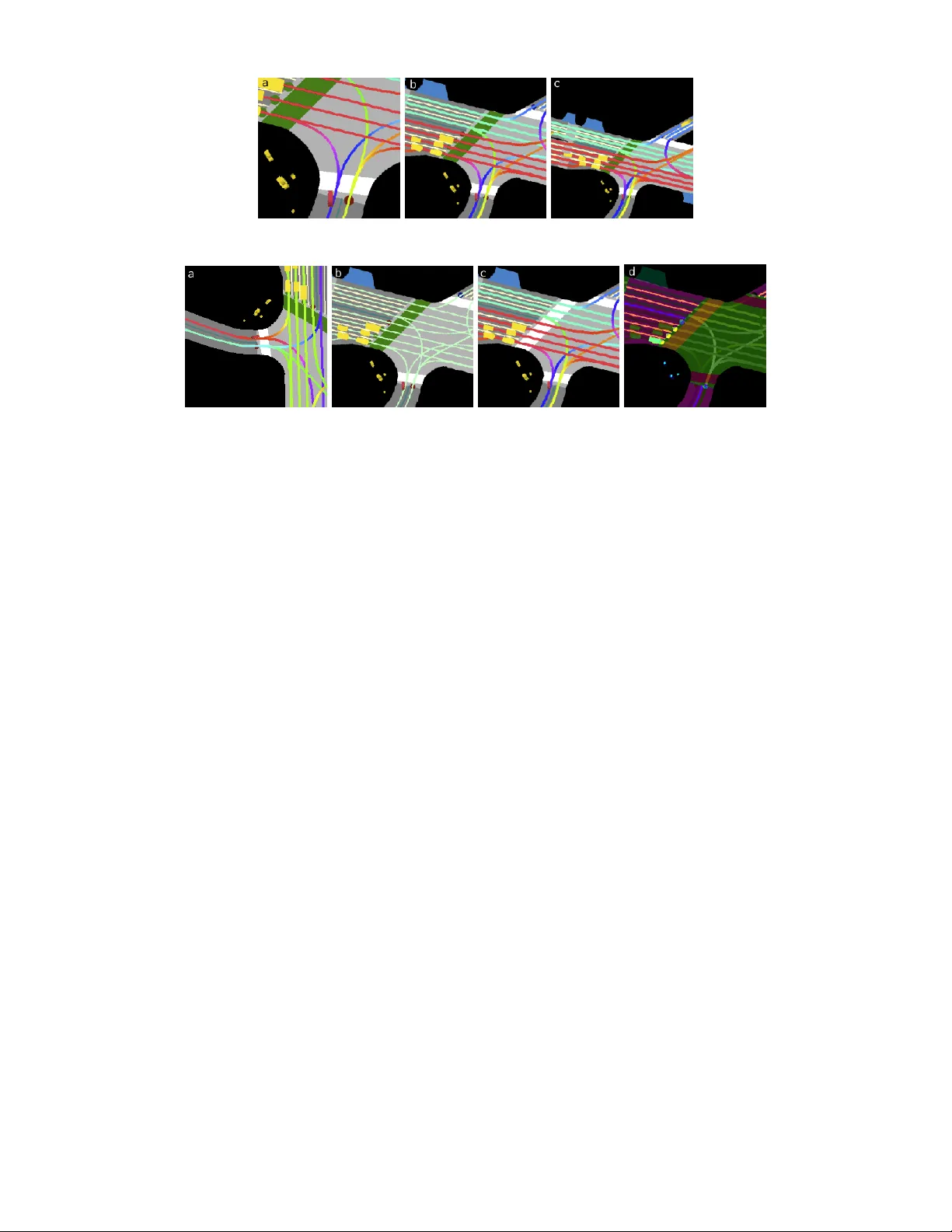
Loading high-quality paper...
Comments & Academic Discussion
Loading comments...
Leave a Comment