Optimizing Neural Networks with Kronecker-factored Approximate Curvature

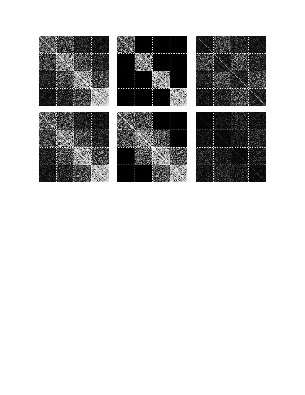
Optimizing Neural Networks with Kroneck er -factored Approximate Curv ature James Martens ∗ and Roger Grosse † Department of Computer Science, Uni versity of T oronto Abstract W e propose an ef ﬁcient method for approximating natural gradient descent in neural net- works which we call Kroneck er-factored Approximate Curvature (K-F A C). K-F A C is based on an efﬁciently in vertible approximation of a neural network’ s Fisher information matrix which is neither diagonal nor lo w-rank, and in some cases is completely non-sparse. It is deri ved by approximating various large blocks of the Fisher (corresponding to entire layers) as being the Kronecker product of two much smaller matrices. While only se v eral times more e xpensiv e to compute than the plain stochastic gradient, the updates produced by K-F A C make much more progress optimizing the objecti ve, which results in an algorithm that can be much faster than stochastic gradient descent with momentum in practice. And unlik e some previously proposed approximate natural-gradient/Ne wton methods which use high-quality non-diagonal curv ature matrices (such as Hessian-free optimization), K-F A C w orks very well in highly stochastic op- timization regimes. This is because the cost of storing and in verting K-F A C’ s approximation to the curv ature matrix does not depend on the amount of data used to estimate it, which is a feature typically associated only with diagonal or low-rank approximations to the curvature matrix. 1 Intr oduction The problem of training neural networks is one of the most important and highly in vestigated ones in machine learning. Despite work on layer-wise pretraining schemes, and various sophisti- cated optimization methods which try to approximate Ne wton-Raphson updates or natural gradi- ent updates, stochastic gradient descent (SGD), possibly augmented with momentum, remains the method of choice for large-scale neural netw ork training (Sutske ver et al., 2013). From the work on Hessian-free optimization (HF) (Martens, 2010) and related methods (e.g. ∗ jmartens@cs.toronto.edu † rgrosse@cs.toronto.edu 1 V inyals and Pov ey, 2012) we know that updates computed using local curvature information can make much more progress per iteration than the scaled gradient. The reason that HF sees fewer practical applications than SGD are twofold. Firstly , its updates are much more expensi v e to com- pute, as the y in volv e running linear conjugate gradient (CG) for potentially hundreds of iterations, each of which requires a matrix-vector product with the curvature matrix (which are as expen- si ve to compute as the stochastic gradient on the current mini-batch). Secondly , HF’ s estimate of the curvature matrix must remain ﬁxed while CG iterates, and thus the method is able to go through much less data than SGD can in a comparable amount of time, making it less well suited to stochastic optimizations. As discussed in Martens and Sutskev er (2012) and Sutske ver et al. (2013), CG has the po- tential to be much faster at local optimization than gradient descent, when applied to quadratic objecti ve functions. Thus, insofar as the objectiv e can be locally approximated by a quadratic, each step of CG could potentially be doing a lot more work than each iteration of SGD, which would result in HF being much faster ov erall than SGD. Ho we ver , there are e xamples of quadratic functions (e.g. Li, 2005), characterized by curvature matrices with highly spread-out eigen value distributions, where CG will hav e no distinct advantage ov er well-tuned gradient descent with momentum. Thus, insofar as the quadratic functions being optimized by CG within HF are of this character , HF shouldn’t in principle be faster than well-tuned SGD with momentum. The ex- tent to which neural network objectiv e functions give rise to such quadratics is unclear , although Sutske ver et al. (2013) pro vides some preliminary evidence that the y do. CG falls victim to this worst-case analysis because it is a ﬁrst-order method. This motiv ates us to consider methods which don’ t rely on ﬁrst-order methods like CG as their primary engines of optimization. One such class of methods which ha ve been widely studied are those which work by directly in verting a diagonal, block-diagonal, or low-rank approximation to the curvature matrix (e.g. Becker and LeCun, 1989; Schaul et al., 2013; Zeiler, 2013; Le Roux et al., 2008; Ollivier, 2013). In fact, a diagonal approximation of the Fisher information matrix is used within HF as a preconditioner for CG. Howe ver , these methods provide only a limited performance improvement in practice, especially compared to SGD with momentum (see for example Schraudolph et al., 2007; Zeiler, 2013), and many practitioners tend to forgo them in fa vor of SGD or SGD with momentum. W e kno w that the curv ature associated with neural network objecti ve functions is highly non- diagonal, and that updates which properly respect and account for this non-diagonal curvature, such as those generated by HF , can make much more progress minimizing the objectiv e than the plain gradient or updates computed from diagonal approximations of the curvature (usually ∼ 10 2 HF updates are required to adequately minimize most objecti ves, compared to the ∼ 10 4 − 10 5 required by methods that use diagonal approximations). Thus, if we had an efﬁcient and direct way to compute the in verse of a high-quality non-diagonal approximation to the curvature matrix (i.e. without relying on ﬁrst-order methods like CG) this could potentially yield an optimization method whose updates would be large and powerful like HF’ s, while being (almost) as cheap to compute as the stochastic gradient. 2 In this work we de velop such a method, which we call Kronecker -factored Approximate Cur - v ature (K-F A C). W e show that our method can be much faster in practice than ev en highly tuned implementations of SGD with momentum on certain standard neural network optimization bench- marks. The main ingredient in K-F A C is a sophisticated approximation to the Fisher information matrix, which despite being neither diagonal nor low-rank, nor e ven block-diagonal with small blocks, can be in verted very ef ﬁciently , and can be estimated in an online fashion using arbitrarily large subsets of the training data (without increasing the cost of in version). This approximation is built in two stages. In the ﬁrst, the rows and columns of the Fisher are di vided into groups, each of which corresponds to all the weights in a given layer , and this gives rise to a block-partitioning of the matrix (where the blocks are much larger than those used by Le Roux et al. (2008) or Olli vier (2013)). These blocks are then approximated as Kronecker products between much smaller matrices, which we show is equiv alent to making certain approximating assumptions regarding the statistics of the netw ork’ s gradients. In the second stage, this matrix is further approximated as ha ving an in verse which is either block-diagonal or block-tridiagonal. W e justify this approximation through a careful examination of the relationships between in verse cov ariances, tree-structured graphical models, and linear re- gression. Notably , this justiﬁcation doesn’t apply to the Fisher itself, and our experiments conﬁrm that while the in verse Fisher does indeed possess this structure (approximately), the Fisher itself does not. The rest of this paper is organized as follo ws. Section 2 giv es basic background and notation for neural networks and the natural gradient. Section 3 describes our initial Kronecker product approximation to the Fisher . Section 4 describes our further block-diagonal and block-tridiagonal approximations of the in verse Fisher , and how these can be used to deriv e an ef ﬁcient in version algorithm. Section 5 describes ho w we compute online estimates of the quantities required by our in verse Fisher approximation ov er a large “windo w” of previously processed mini-batches (which makes K-F A C very different from methods like HF or KSD, which base their estimates of the curv ature on a single mini-batch). Section 6 describes ho w we use our approximate Fisher to obtain a practical and rob ust optimization algorithm which requires v ery little manual tuning, through the careful application of various theoretically well-founded “damping” techniques that are standard in the optimization literature. Note that damping techniques compensate both for the local quadratic approximation being implicitly made to the objecti ve, and for our further approximation of the Fisher , and are non-optional for essentially any 2nd-order method like K-F A C to work properly , as is well established by both theory and practice within the optimization literature (Nocedal and Wright, 2006). Section 7 describes a simple and ef fecti ve way of adding a type of “momentum” to K-F A C, which we have found works very well in practice. Section 8 describes the computational costs associated with K-F A C, and various ways to reduce them to the point where each update is at most only sev eral times more expensiv e to compute than the stochastic gradient. Section 9 giv es complete high-lev el pseudocode for K-F A C. Section 10 characterizes a broad class of network transformations and reparameterizations to which K-F A C is essentially in v ariant. Section 3 11 considers some related prior methods for neural network optimization. Proofs of formal results are located in the appendix. 2 Backgr ound and notation 2.1 Neural Networks In this section we will deﬁne the basic notation for feed-forward neural networks which we will use throughout this paper . Note that this presentation closely follo ws the one from Martens (2014). A neural network transforms its input a 0 = x to an output f ( x, θ ) = a ` through a series of ` layers, each of which consists of a bank of units/neurons. The units each receiv e as input a weighted sum of the outputs of units from the previous layer and compute their output via a nonlinear “activ ation” function. W e denote by s i the vector of these weighted sums for the i -th layer , and by a i the v ector of unit outputs (aka “acti vities”). The precise computation performed at each layer i ∈ { 1 , . . . , ` } is gi ven as follo ws: s i = W i ¯ a i − 1 a i = φ i ( s i ) where φ i is an element-wise nonlinear function, W i is a weight matrix, and ¯ a i is deﬁned as the vector formed by appending to a i an additional homogeneous coordinate with value 1. Note that we do not include explicit bias parameters here as these are captured implicitly through our use of homogeneous coordinates. In particular , the last column of each weight matrix W i corresponds to what is usually thought of as the “bias vector”. Figure 1 illustrates our deﬁnition for ` = 2 . W e will deﬁne θ = [vec( W 1 ) > v ec( W 2 ) > . . . v ec( W ` ) > ] > , which is the vector consisting of all of the network’ s parameters concatenated together , where vec is the operator which vectorizes matrices by stacking their columns together . W e let L ( y , z ) denote the loss function which measures the disagreement between a prediction z made by the network, and a target y . The training objective function h ( θ ) is the av erage (or expectation) of losses L ( y , f ( x, θ )) with respect to a training distribution ˆ Q x,y ov er input-target pairs ( x, y ) . h ( θ ) is a proxy for the objectiv e which we actually care about but don’t hav e access to, which is the expectation of the loss tak en with respect to the true data distribution Q x,y . W e will assume that the loss is giv en by the negati ve log probability associated with a simple predicti ve distrib ution R y | z for y parameterized by z , i.e. that we have L ( y , z ) = − log r ( y | z ) where r is R y | z ’ s density function. This is the case for both the standard least-squares and cross- entropy objectiv e functions, where the predictive distributions are multi variate normal and multi- nomial, respecti vely . 4 W e will let P y | x ( θ ) = R y | f ( x,θ ) denote the conditional distribution deﬁned by the neural net- work, as parameterized by θ , and p ( y | x, θ ) = r ( y | f ( x, θ )) its density function. Note that minimiz- ing the objecti ve function h ( θ ) can be seen as maximum likelihood learning of the model P y | x ( θ ) . For con venience we will deﬁne the follo wing additional notation: D v = d L ( y , f ( x, θ )) d v = − d log p ( y | x, θ ) d v and g i = D s i Algorithm 1 shows how to compute the gradient D θ of the loss function of a neural network using standard backpropagation. Algorithm 1 An algorithm for computing the gradient of the loss L ( y , f ( x, θ )) for a giv en ( x, y ) . Note that we are assuming here for simplicity that the φ i are deﬁned as coordinate-wise functions. input: a 0 = x ; θ mapped to ( W 1 , W 2 , . . . , W ` ) . /* Forw ard pass */ f or all i fr om 1 to ` do s i ← W i ¯ a i − 1 a i ← φ i ( s i ) end f or /* Loss deri vati ve computation */ D a ` ← ∂ L ( y , z ) ∂ z     z = a ` /* Backwards pass */ f or all i fr om ` downto 1 do g i ← D a i  φ 0 i ( s i ) D W i ← g i ¯ a > i − 1 D a i − 1 ← W > i g i end f or output: D θ = [vec( D W 1 ) > v ec( D W 2 ) > . . . v ec( D W ` ) > ] > 5 Figure 1: A depiction of a standard feed-forward neural network for ` = 2 . 2.2 The Natural Gradient Because our network deﬁnes a conditional model P y | x ( θ ) , it has an associated Fisher information matrix (which we will simply call “the Fisher”) which is gi ven by F = E " d log p ( y | x, θ ) d θ d log p ( y | x, θ ) d θ > # = E[ D θ D θ > ] Here, the expectation is taken with respect to the data distribution Q x ov er inputs x , and the model’ s predicti ve distribution P y | x ( θ ) over y . Since we usually don’t hav e access to Q x , and the abov e expectation would likely be intractable e v en if we did, we will instead compute F using the training distribution ˆ Q x ov er inputs x . The well-kno wn natural gradient (Amari, 1998) is deﬁned as F − 1 ∇ h ( θ ) . Moti vated from the perspecti ve of information geometry (Amari and Nagaoka, 2000), the natural gradient deﬁnes the direction in parameter space which giv es the largest change in the objectiv e per unit of change in the model, as measured by the KL-div ergence. This is to be contrasted with the standard gradient, which can be deﬁned as the direction in parameter space which gives the largest change in the objecti ve per unit of change in the parameters, as measured by the standard Euclidean metric. The natural gradient also has links to sev eral classical ideas from optimization. It can be sho wn (Martens, 2014; Pascanu and Bengio, 2014) that the Fisher is equiv alent to the General- ized Gauss-Newton matrix (GGN) (Schraudolph, 2002; Martens and Sutske ver, 2012) in certain important cases, which is a well-kno wn positi ve semi-deﬁnite approximation to the Hessian of the objecti ve function. In particular , (Martens, 2014) sho wed that when the GGN is deﬁned so that the 6 network is linearized up to the loss function, and the loss function corresponds to the negati ve log probability of observations under an e xponential family model R y | z with z representing the natur al parameter s , then the Fisher corresponds exactly to the GGN. 1 The GGN has served as the curvature matrix of choice in HF and related methods, and so in light of its equiv alence to the Fisher , these 2nd-order methods can be seen as approximate natural gradient methods. And perhaps more importantly from a practical perspecti ve, natural gradient- based optimization methods can con versely be viewed as 2nd-order optimization methods, which as pointed out by Martens (2014)), brings to bare the v ast wisdom that has accumulated about ho w to make such methods work well in both theory and practice (e.g Nocedal and Wright, 2006). In Section 6 we producti vely make use of these connections in order to design a robust and highly ef fectiv e optimization method using our approximation to the natural gradient/Fisher (which is de veloped in Sections 3 and 4). For some good recent discussion and analysis of the natural gradient, see Arnold et al. (2011); Martens (2014); Pascanu and Bengio (2014). 3 A block-wise Kr onecker -factored Fisher appr oximation The main computational challenge associated with using the natural gradient is computing F − 1 (or its product with ∇ h ). For large networks, with potentially millions of parameters, computing this in verse nai vely is computationally impractical. In this section we de v elop an initial approximation of F which will be a key ingredient in deri ving our ef ﬁciently computable approximation to F − 1 and the natural gradient. Note that D θ = [vec( D W 1 ) > v ec( D W 2 ) > · · · v ec( D W ` ) > ] > and so F can be expressed as F = E  D θ D θ >  = E  [v ec( D W 1 ) > v ec( D W 2 ) > · · · v ec( D W ` ) > ] > [v ec( D W 1 ) > v ec( D W 2 ) > · · · v ec( D W ` ) > ]  =      E  v ec( D W 1 ) v ec( D W 1 ) >  E  v ec( D W 1 ) v ec( D W 2 ) >  · · · E  v ec( D W 1 ) v ec( D W ` ) >  E  v ec( D W 2 ) v ec( D W 1 ) >  E  v ec( D W 2 ) v ec( D W 2 ) >  · · · E  v ec( D W 2 ) v ec( D W ` ) >  . . . . . . . . . . . . E  v ec( D W ` ) v ec( D W 1 ) >  E  v ec( D W ` ) v ec( D W 2 ) >  · · · E  v ec( D W ` ) v ec( D W ` ) >       Thus, we see that F can be vie wed as an ` by ` block matrix, with the ( i, j ) -th block F i,j gi ven by F i,j = E  v ec( D W i ) v ec( D W j ) >  . 1 Note that the condition that z represents the natural parameters might require one to formally include the nonlinear transformation usually performed by the ﬁnal nonlinearity φ ` of the network (such as the logistic-sigmoid transform before a cross-entropy error) as part of the loss function L instead. Equiv alently , one could linearize the network only up to the input s ` to φ ` when computing the GGN (see Martens and Sutske ver (2012)). 7 Noting that D W i = g i ¯ a > i − 1 and that vec( uv > ) = v ⊗ u we hav e v ec( D W i ) = v ec( g i ¯ a > i − 1 ) = ¯ a i − 1 ⊗ g i , and thus we can re write F i,j as F i,j = E  v ec( D W i ) v ec( D W j ) >  = E  (¯ a i − 1 ⊗ g i )(¯ a j − 1 ⊗ g j ) >  = E  (¯ a i − 1 ⊗ g i )(¯ a > j − 1 ⊗ g > j )  = E  ¯ a i − 1 ¯ a > j − 1 ⊗ g i g > j  where A ⊗ B denotes the Kronecker product between A ∈ R m × n and B , and is gi ven by A ⊗ B ≡    [ A ] 1 , 1 B · · · [ A ] 1 ,n B . . . . . . . . . [ A ] m, 1 B · · · [ A ] m,n B    Note that the Kronecker product satisﬁes many con venient properties that we will make use of in this paper , especially the identity ( A ⊗ B ) − 1 = A − 1 ⊗ B − 1 . See V an Loan (2000) for a good discussion of the Kronecker product. Our initial approximation ˜ F to F will be deﬁned by the follo wing block-wise approximation: F i,j = E  ¯ a i − 1 ¯ a > j − 1 ⊗ g i g > j  ≈ E  ¯ a i − 1 ¯ a > j − 1  ⊗ E  g i g > j  = ¯ A i − 1 ,j − 1 ⊗ G i,j = ˜ F i,j (1) where ¯ A i,j = E  ¯ a i ¯ a > j  and G i,j = E  g i g > j  . This gi ves ˜ F =      ¯ A 0 , 0 ⊗ G 1 , 1 ¯ A 0 , 1 ⊗ G 1 , 2 · · · ¯ A 0 ,` − 1 ⊗ G 1 ,` ¯ A 1 , 0 ⊗ G 2 , 1 ¯ A 1 , 1 ⊗ G 2 , 2 · · · ¯ A 1 ,` − 1 ⊗ G 2 ,` . . . . . . . . . . . . ¯ A ` − 1 , 0 ⊗ G `, 1 ¯ A ` − 1 , 1 ⊗ G `, 2 · · · ¯ A ` − 1 ,` − 1 ⊗ G `,`      which has the form of what is kno wn as a Khatri-Rao product in multiv ariate statistics. The expectation of a Kronecker product is, in general, not equal to the Kronecker product of expectations, and so this is indeed a major approximation to mak e, and one which lik ely won’ t be- come e xact under an y realistic set of assumptions, or as a limiting case in some kind of asymptotic analysis. Nev ertheless, it seems to be fairly accurate in practice, and is able to successfully capture the “coarse structure” of the Fisher , as demonstrated in Figure 2 for an example netw ork. As we will see in later sections, this approximation leads to signiﬁcant computational sa vings in terms of storage and in version, which we will be able to leverage in order to design an efﬁcient algorithm for computing an approximation to the natural gradient. 3.1 Interpr etations of this approximation Consider an arbitrary pair of weights [ W i ] k 1 ,k 2 and [ W j ] k 3 ,k 4 from the network, where [ · ] i,j denotes the v alue of the ( i, j ) -th entry . W e have that the corresponding deriv ati ves of these weights are 8 Figure 2: A comparison of the exact Fisher F and our block-wise Kronecker-factored approximation ˜ F , for the middle 4 layers of a standard deep neural network partially trained to classify a 16x16 do wn-scaled version of MNIST . The network was trained with 7 iterations of K-F AC in batch mode, achie ving 5% error (the error reached 0% after 22 iterations) . The network architecture is 256-20-20-20-20-20-10 and uses standard tanh units. On the left is the exact Fisher F , in the middle is our approximation ˜ F , and on the right is the difference of these. The dashed lines delineate the blocks. Note that for the purposes of visibility we plot the absolute v alues of the entries, with the white le vel corresponding linearly to the size of these v alues (up to some maximum, which is the same in each image). gi ven by D [ W i ] k 1 ,k 2 = ¯ a (1) g (1) and D [ W j ] k 3 ,k 4 = ¯ a (2) g (2) , where we denote for con v enience ¯ a (1) = [¯ a i − 1 ] k 1 , ¯ a (2) = [¯ a j − 1 ] k 3 , g (1) = [ g i ] k 2 , and g (2) = [ g j ] k 4 . The approximation giv en by eqn. 1 is equi valent to making the following approximation for each pair of weights: E [ D [ W i ] k 1 ,k 2 D [ W j ] k 3 ,k 4 ] = E  (¯ a (1) g (1) )(¯ a (2) g (2) )  = E  ¯ a (1) ¯ a (2) g (1) g (2)  ≈ E  ¯ a (1) ¯ a (2)  E  g (1) g (2)  (2) And thus one way to interpret the approximation in eqn. 1 is that we are assuming statistical inde- pendence between products ¯ a (1) ¯ a (2) of unit acti vities and products g (1) g (2) of unit input deri v ativ es. Another more detailed interpretation of the approximation emerges by considering the follo w- ing e xpression for the approximation error E  ¯ a (1) ¯ a (2) g (1) g (2)  − E  ¯ a (1) ¯ a (2)  E  g (1) g (2)  (which is deri ved in the appendix): κ (¯ a (1) , ¯ a (2) , g (1) , g (2) ) + E[¯ a (1) ] κ (¯ a (2) , g (1) , g (2) ) + E[¯ a (2) ] κ (¯ a (1) , g (1) , g (2) ) (3) Here κ ( · ) denotes the cumulant of its arguments. Cumulants are a natural generalization of the concept of mean and v ariance to higher orders, and indeed 1st-order cumulants are means and 2nd-order cumulants are cov ariances. Intuitiv ely , cumulants of order k measure the degree to which the interaction between v ariables is intrinsically of order k , as opposed to arising from man y lo wer-order interactions. A basic upper bound for the approximation error is | κ (¯ a (1) , ¯ a (2) , g (1) , g (2) ) | + | E[ ¯ a (1) ] || κ (¯ a (2) , g (1) , g (2) ) | + | E[ ¯ a (2) ] || κ (¯ a (1) , g (1) , g (2) ) | (4) 9 which will be small if all of the higher-order cumulants are small (i.e. those of order 3 or higher). Note that in principle this upper bound may be loose due to possible cancellations between the terms in eqn. 3. Because higher-order cumulants are zero for variables jointly distributed according to a mul- ti variate Gaussian, it follo ws that this upper bound on the approximation error will be small insofar as the joint distribution over ¯ a (1) , ¯ a (2) , g (1) , and g (2) is well approximated by a multi variate Gaus- sian. And while we are not aw are of an argument for why this should be the case in practice, it does seem to be the case that for the example network from Figure 2, the size of the error is well predicted by the size of the higher-order cumulants. In particular , the total approximation error , summed ov er all pairs of weights in the middle 4 layers, is 2894 . 4 , and is of roughly the same size as the corresponding upper bound ( 4134 . 6 ), whose size is tied to that of the higher order cumulants (due to the impossibility of cancellations in eqn. 4). 4 Additional appr oximations to ˜ F and in v erse computations T o the best of our kno wledge there is no efﬁcient general method for in v erting a Khatri-Rao product like ˜ F . Thus, we must mak e further approximations if we hope to obtain an ef ﬁciently computable approximation of the in verse Fisher . In the following subsections we argue that the in verse of ˜ F can be reasonably approximated as ha ving one of two special structures, either of which mak e it ef ﬁciently computable. The second of these will be slightly less restrictiv e than the ﬁrst (and hence a better approximation) at the cost of some additional complexity . W e will then show how matrix-vector products with these approximate in verses can be efﬁciently computed, which will thus giv e an efﬁcient algorithm for computing an approximation to the natural gradient. 4.1 Structur ed in verses and the connection to linear r egr ession Suppose we are gi ven a multi variate distrib ution whose associated co variance matrix is Σ . Deﬁne the matrix B so that for i 6 = j , [ B ] i,j is the coef ﬁcient on the j -th v ariable in the optimal linear predictor of the i -th variable from all the other v ariables, and for i = j , [ B ] i,j = 0 . Then deﬁne the matrix D to be the diagonal matrix where [ D ] i,i is the variance of the error associated with such a predictor of the i -th v ariable. Pourahmadi (2011) sho wed that B and D can be obtained from the in verse cov ariance Σ − 1 by the formulas [ B ] i,j = − [Σ − 1 ] i,j [Σ − 1 ] i,i and [ D ] i,i = 1 [Σ − 1 ] i,i 10 from which it follo ws that the in verse co variance matrix can be e xpressed as Σ − 1 = D − 1 ( I − B ) Intuiti vely , this result says that each row of the in verse cov ariance Σ − 1 is giv en by the coefﬁ- cients of the optimal linear predictor of the i -th variable from the others, up to a scaling factor . So if the j -th variable is much less “useful” than the other variables for predicting the i -th variable, we can expect that the ( i, j ) -th entry of the inv erse cov ariance will be relati vely small. Note that “usefulness” is a subtle property as we have informally deﬁned it. In particular , it is not equiv alent to the degree of correlation between the j -th and i -th v ariables, or any such simple measure. As a simple example, consider the case where the j -th variable is equal to the k -th variable plus independent Gaussian noise. Since any linear predictor can achiev e a lo wer v ariance simply by shifting weight from the j -th v ariable to the k -th v ariable, we ha ve that the j -th v ariable is not useful (and its coef ﬁcient will thus be zero) in the task of predicting the i -th v ariable for any setting of i other than i = j or i = k . Noting that the Fisher F is a co v ariance matrix o ver D θ w .r .t. the model’ s distribution (because E[ D θ ] = 0 by Lemma 4), we can thus apply the abov e analysis to the distribution ov er D θ to gain insight into the approximate structure of F − 1 , and by extension its approximation ˜ F − 1 . Consider the deriv ati ve D W i of the loss with respect to the weights W i of layer i . Intuitiv ely , if we are trying to predict one of the entries of D W i from the other entries of D θ , those entries also in D W i will likely be the most useful in this regard. Thus, it stands to reason that the largest entries of ˜ F − 1 will be those on the diagonal blocks, so that ˜ F − 1 will be well approximated as block-diagonal, with each block corresponding to a dif ferent D W i . Beyond the other entries of D W i , it is the entries of D W i +1 and D W i − 1 (i.e. those associated with adjacent layers) that will arguably be the most useful in predicting a giv en entry of D W i . This is because the true process for computing the loss gradient only uses information from the layer belo w (during the forward pass) and from the layer abo ve (during the backw ards pass). Thus, approximating ˜ F − 1 as block-tridiagonal seems lik e a reasonable and milder alternati ve than taking it to be block-diagonal. Indeed, this approximation would be exact if the distrib ution over D θ were giv en by a directed graphical model which generated each of the D W i ’ s, one layer at a time, from either D W i +1 or D W i − 1 . Or equi v alently , if D W i were distrib uted according to an undirected Gaussian graphical model with binary potentials only between entries in the same or adjacent layers. Both of these models are depicted in Figure 4. No w while in reality the D W i ’ s are generated using information from adjacent layers accord- ing to a process that is neither linear nor Gaussian , it nonetheless stands to reason that their joint statistics might be reasonably approximated by such a model. In fact, the idea of approximating the distrib ution over loss gradients with a directed graphical model forms the basis of the recent F ANG method of Grosse and Salakhutdinov (2015). Figure 3 e xamines the extent to which the in verse Fisher is well approximated as block- diagonal or block-tridiagonal for an example netw ork. 11 Figure 3: A comparison of our block-wise Kronecker-factored approximation ˜ F , and its in verse, using the example neural network from Figure 2. On the left is ˜ F , in the middle is its exact in verse, and on the right is a 4x4 matrix containing the a verages of the absolute v alues of the entries in each block of the in verse. As predicted by our theory , the in verse exhibits an approximate block-tridiagonal structure, whereas ˜ F itself does not. Note that the corresponding plots for the exact F and its inv erse look similar . The very small blocks visible on the diagonal of the inv erse each correspond to the weights on the outgoing connections of a particular unit. The in verse was computed subject to the factored T ikhonov damping technique described in Sections 6.3 and 6.6, using the same value of γ that was used by K-F A C at the iteration from which this example was tak en (see Figure 2). Note that for the purposes of visibility we plot the absolute v alues of the entries, with the white level corresponding linearly to the size of these values (up to some maximum, which is chosen differently for the Fisher approximation and its in verse, due to the highly differing scales of these matrices). 12 In the follo wing tw o subsections we sho w ho w both the block-diagonal and block-tridiagonal approximations to ˜ F − 1 gi ve rise to computationally ef ﬁcient methods for computing matrix-vector products with it. And at the end of Section 4 we present two ﬁgures (Figures 5 and 6) which examine the quality of these approximations for an e xample network. 4.2 A pproximating ˜ F − 1 as block-diagonal Approximating ˜ F − 1 as block-diagonal is equi v alent to approximating ˜ F as block-diagonal. A natural choice for such an approximation ˘ F of ˜ F , is to take the block-diagonal of ˘ F to be that of ˜ F . This gi ves the matrix ˘ F = diag  ˜ F 1 , 1 , ˜ F 2 , 2 , . . . , , ˜ F `,`  = diag  ¯ A 0 , 0 ⊗ G 1 , 1 , ¯ A 1 , 1 ⊗ G 2 , 2 , . . . , ¯ A ` − 1 ,` − 1 ⊗ G `,`  Using the identity ( A ⊗ B ) − 1 = A − 1 ⊗ B − 1 we can easily compute the in verse of ˘ F as ˘ F − 1 = diag  ¯ A − 1 0 , 0 ⊗ G − 1 1 , 1 , ¯ A − 1 1 , 1 ⊗ G − 1 2 , 2 , . . . , ¯ A − 1 ` − 1 ,` − 1 ⊗ G − 1 `,`  Thus, computing ˘ F − 1 amounts to computing the in verses of 2 ` smaller matrices. Then to compute u = ˘ F − 1 v , we can make use of the well-kno wn identity ( A ⊗ B ) vec( X ) = v ec( B X A > ) to get U i = G − 1 i,i V i ¯ A − 1 i − 1 ,i − 1 where v maps to ( V 1 , V 2 , . . . , V ` ) and u maps to ( U 1 , U 2 , . . . , U ` ) in an analogous way to how θ maps to ( W 1 , W 2 , . . . , W ` ) . Note that block-diagonal approximations to the Fisher information hav e been proposed before in TONGA (Le Roux et al., 2008), where each block corresponds to the weights associated with a particular unit. In our block-diagonal approximation, the blocks correspond to all the parameters in a giv en layer , and are thus much larger . In fact, they are so large that they would be impractical to in vert as general matrices. 4.3 A pproximating ˜ F − 1 as block-tridiagonal Note that unlike in the above block-diagonal case, approximating ˜ F − 1 as block-tridiagonal is not equi valent to approximating ˜ F as block-tridiagonal. Thus we require a more sophisticated ap- proach to deal with such an approximation. W e de velop such an approach in this subsection. T o start, we will deﬁne ˆ F to be the matrix which agrees with ˜ F on the tridiagonal blocks, and which satisﬁes the property that ˆ F − 1 is block-tridiagonal. Note that this deﬁnition implies certain v alues for the off-tridiagonal blocks of ˆ F which will differ from those of ˜ F insofar as ˜ F − 1 is not actually block-tridiagonal. 13 . . . . . . Figure 4: A diagram depicting the UGGM corresponding to ˆ F − 1 and its equi v alent DGGM. The UGGM’ s edges are labeled with the corresponding weights of the model (these are distinct from the network’ s weights). Here, ( ˆ F − 1 ) i,j denotes the ( i, j ) -th block of ˆ F − 1 . The DGGM’ s edges are labeled with the matrices that specify the linear mapping from the source node to the conditional mean of the destination node (whose conditional cov ariance is gi ven by its label). T o establish that such a matrix ˆ F is well deﬁned and can be in verted efﬁciently , we ﬁrst observe that assuming that ˆ F − 1 is block-tridiagonal is equiv alent to assuming that it is the preci- sion matrix of an undirected Gaussian graphical model (UGGM) ov er D θ (as depicted in Figure 4), whose density function is proportional to exp( −D θ > ˆ F − 1 D θ ) . As this graphical model has a tree structure, there is an equiv alent directed graphical model with the same distribution and the same (undirected) graphical structure (e.g. Bishop, 2006), where the directionality of the edges is gi ven by a directed acyclic graph (D A G). Moreov er , this equi valent directed model will also be linear/Gaussian, and hence a directed Gaussian Graphical model (DGGM). Next we will show ho w the parameters of such a DGGM corresponding to ˆ F can be efﬁciently recov ered from the tridiagonal blocks of ˆ F , so that ˆ F is uniquely determined by these blocks (and hence well-deﬁned). W e will assume here that the direction of the edges is from the higher layers to the lo wer ones. Note that a different choice for these directions would yield a superﬁcially dif ferent algorithm for computing the in verse of ˆ F that would nonetheless yield the same output. For each i , we will denote the conditional co variance matrix of v ec( D W i ) on v ec( D W i +1 ) by Σ i | i +1 and the linear coef ﬁcients from vec( D W i +1 ) to vec( D W i ) by the matrix Ψ i,i +1 , so that the conditional distributions deﬁning the model are v ec( D W i ) ∼ N  Ψ i,i +1 v ec( D W i +1 ) , Σ i | i +1  and v ec( D W ` ) ∼ N  ~ 0 , Σ `  Since Σ ` is just the covariance of v ec( D W ` ) , it is giv en simply by ˆ F `,` = ˜ F `,` . And for i ≤ ` − 1 , we can see that Ψ i,i +1 is gi ven by Ψ i,i +1 = ˆ F i,i +1 ˆ F − 1 i +1 ,i +1 = ˜ F i,i +1 ˜ F − 1 i +1 ,i +1 =  ¯ A i − 1 ,i ⊗ G i,i +1   ¯ A i,i ⊗ G i +1 ,i +1  − 1 = Ψ ¯ A i − 1 ,i ⊗ Ψ G i,i +1 14 where Ψ ¯ A i − 1 ,i = ¯ A i − 1 ,i ¯ A − 1 i,i and Ψ G i,i +1 = G i,i +1 G − 1 i +1 ,i +1 The conditional cov ariance Σ i | i +1 is thus gi ven by Σ i | i +1 = ˆ F i,i − Ψ i,i +1 ˆ F i +1 ,i +1 Ψ > i,i +1 = ˜ F i,i − Ψ i,i +1 ˜ F i +1 ,i +1 Ψ > i,i +1 = ¯ A i − 1 ,i − 1 ⊗ G i,i − Ψ ¯ A i − 1 ,i ¯ A i,i Ψ ¯ A > i − 1 ,i ⊗ Ψ G i,i +1 G i +1 ,i +1 Ψ G > i,i +1 Follo wing the work of Grosse and Salakhutdinov (2015), we use the block generalization of well-kno wn “Cholesky” decomposition of the precision matrix of DGGMs (Pourahmadi, 1999), which gi ves ˆ F − 1 = Ξ > ΛΞ where, Λ = diag  Σ − 1 1 | 2 , Σ − 1 2 | 3 , . . . , Σ − 1 ` − 1 | ` , Σ − 1 `  and Ξ =        I − Ψ 1 , 2 I − Ψ 2 , 3 I . . . . . . − Ψ ` − 1 ,` I        Thus, matrix-vector multiplication with ˆ F − 1 amounts to performing matrix-vector multipli- cation by Ξ , follo wed by Λ , and then by Ξ > . As in the block-diagonal case considered in the previous subsection, matrix-vector products with Ξ (and Ξ > ) can be ef ﬁciently computed using the well-known identity ( A ⊗ B ) − 1 = A − 1 ⊗ B − 1 . In particular , u = Ξ > v can be computed as U i = V i − Ψ G > i − 1 ,i V i − 1 Ψ ¯ A i − 2 ,i − 1 and U 1 = V 1 and similarly u = Ξ v can be computed as U i = V i − Ψ G i,i +1 V i +1 Ψ ¯ A > i − 1 ,i and U ` = V ` where the U i ’ s and V i ’ s are deﬁned in terms of u and v as in the pre vious subsection. Multiplying a v ector v by Λ amounts to multiplying each vec( V i ) by the corresponding Σ − 1 i | i +1 . This is slightly trick y because Σ i | i +1 is the dif ference of Kronecker products, so we cannot use the straightforward identity ( A ⊗ B ) − 1 = A − 1 ⊗ B − 1 . Fortunately , there are efﬁcient techniques for in verting such matrices which we discuss in detail in Appendix B. 15 4.4 Examining the appr oximation quality Figures 5 and 6 examine the quality of the approximations ˘ F and ˆ F of ˜ F , which are deriv ed by approximating ˜ F − 1 as block-diagonal and block-tridiagonal (resp.), for an example netw ork. From Figure 5, which compares ˘ F and ˆ F directly to ˜ F , we can see that while ˘ F and ˆ F exactly capture the diagonal and tridiagonal blocks (resp.) of ˜ F , as they must by deﬁnition, ˆ F ends up approximating the of f-tridiagonal blocks of ˜ F very well too. This is likely o wed to the fact that the approximating assumption used to deri v e ˆ F , that ˜ F − 1 is block-tridiagonal, is a very reasonable one in practice (judging by Figure 3). Figure 6, which compares ˘ F − 1 and ˆ F − 1 to ˜ F − 1 , paints an arguably more interesting and rele vant picture, as the quality of the approximation of the natural gradient will be roughly propor - tional 2 to the quality of approximation of the inver se Fisher . W e can see from this ﬁgure that due to the approximate block-diagonal structure of ˜ F − 1 , ˘ F − 1 is actually a reasonably good approxima- tion of ˜ F − 1 , despite ˘ F being a rather poor approximation of ˜ F (based on Figure 5). Meanwhile, we can see that by accounting for the tri-diagonal blocks, ˆ F − 1 is indeed a signiﬁcantly better approximation of ˜ F − 1 than ˘ F − 1 is, e ven on the diagonal blocks. 2 The error in any approximation F − 1 0 ∇ h of the natural gradient F − 1 ∇ h will be roughly proportional to the error in the approximation F − 1 0 of the associated in verse Fisher F − 1 , since k F − 1 ∇ h − F − 1 0 ∇ h k ≤ k∇ h kk F − 1 − F − 1 0 k . 16 Figure 5: A comparison of our block-wise Kronecker-f actored approximation ˜ F , and its approximations ˘ F and ˆ F (which are based on approximating the in verse ˜ F − 1 as either block-diagonal or block-tridiagonal, respecti vely), using the example neural network from Figure 2. On the left is ˜ F , in the middle its approx- imation, and on the right is the absolute difference of these. The top ro w compares to ˘ F and the bottom ro w compares to ˆ F . While the diagonal blocks of the top right matrix, and the tridiagonal blocks of the bottom right matrix are exactly zero due to ho w ˘ F and ˆ F (resp.) are constructed, the off-tridiagonal blocks of the bottom right matrix, while being very close to zero, are actually non-zero (which is hard to see from the plot). Note that for the purposes of visibility we plot the absolute values of the entries, with the white le vel corresponding linearly to the size of these values (up to some maximum, which is the same in each image). 17 Figure 6: A comparison of the exact in verse ˜ F − 1 of our block-wise Kronecker -factored approximation ˜ F , and its block-diagonal and block-tridiagonal approximations ˘ F − 1 and ˆ F − 1 (resp.), using the example neural network from Figure 2. On the left is ˜ F − 1 , in the middle its approximation, and on the right is the absolute dif ference of these. The top r ow compares to ˘ F − 1 and the bottom row compares to ˆ F − 1 . The inv erse was computed subject to the factored T ikhonov damping technique described in Sections 6.3 and 6.6, using the same value of γ that was used by K-F A C at the iteration from which this example was taken (see Figure 2). Note that for the purposes of visibility we plot the absolute values of the entries, with the white lev el corresponding linearly to the size of these values (up to some maximum, which is the same in each image). 5 Estimating the r equired statistics Recall that ¯ A i,j = E  ¯ a i ¯ a > j  and G i,j = E  g i g > j  . Both approximate Fisher inv erses discussed in Section 4 require some subset of these. In particular , the block-diagonal approximation requires them for i = j , while the block-tridiagonal approximation requires them for j ∈ { i, i + 1 } (noting that ¯ A > i,j = ¯ A j,i and G > i,j = G j,i ). Since the ¯ a i ’ s don’t depend on y , we can take the expectation E  ¯ a i ¯ a > j  with respect to just the training distribution ˆ Q x ov er the inputs x . On the other hand, the g i ’ s do depend on y , and so the expectation 3 E  g i g > j  must be taken with respect to both ˆ Q x and the network’ s predictiv e 3 It is important to note this expectation should not be taken with respect to the training/data distrib ution o ver y (i.e. 18 distribution P y | x . While computing matrix-vector products with the G i,j could be done exactly and efﬁciently for a giv en input x (or small mini-batch of x ’ s) by adapting the methods of Schraudolph (2002), there doesn’t seem to be a sufﬁciently efﬁcient method for computing the entire matrix itself. Indeed, the hardness results of Martens et al. (2012) suggest that this would require, for each example x in the mini-batch, work that is asymptotically equi valent to matrix-matrix multiplication in v olving matrices the same size as G i,j . While a small constant number of such multiplications is arguably an acceptable cost (see Section 8), a number which gro ws with the size of the mini-batch would not be. Instead, we will approximate the expectation over y by a standard Monte-Carlo estimate ob- tained by sampling y ’ s from the network’ s predicti ve distribution and then rerunning the backwards phase of backpropagation (see Algorithm 1) as if these were the training tar gets. Note that computing/estimating the required ¯ A i,j / G i,j ’ s in volv es computing av erages over outer products of v arious ¯ a i ’ s from netw ork’ s usual forward pass, and g i ’ s from the modiﬁed back- wards pass (with tar gets sampled as abov e). Thus we can compute/estimate these quantities on the same input data used to compute the gradient ∇ h , at the cost of one or more additional backwards passes, and a few additional outer -product a verages. Fortunately , this turns out to be quite inexpen- si ve, as we hav e found that just one modiﬁed backwards pass is sufﬁcient to obtain a good quality estimate in practice, and the required outer-product av erages are similar to those already used to compute the gradient in the usual backpropagation algorithm. In the case of online/stochastic optimization we ha ve found that the best strategy is to maintain running estimates of the required ¯ A i,j ’ s and G i,j ’ s using a simple e xponentially decaying averaging scheme. In particular , we take the new running estimate to be the old one weighted by  , plus the estimate on the new mini-batch weighted by 1 −  , for some 0 ≤  < 1 . In our experiments we used  = min { 1 − 1 /k , 0 . 95 } , where k is the iteration number . Note that the more naiv e av eraging scheme where the estimates from each iteration are giv en equal weight would be inappropriate here. This is because the ¯ A i,j ’ s and G i,j ’ s depend on the network’ s parameters θ , and these will slowly change ov er time as optimization proceeds, so that estimates computed many iterations ago will become stale. This kind of exponentially decaying averaging scheme is commonly used in methods in volv- ing diagonal or block-diagonal approximations (with much smaller blocks than ours) to the curv a- ture matrix (e.g. LeCun et al., 1998; Park et al., 2000; Schaul et al., 2013). Such schemes hav e the desirable property that they allo w the curv ature estimate to depend on much more data than can be ˆ Q y | x or Q y | x ). Using the training/data distribution for y would perhaps gi ve an approximation to a quantity known as the “empirical Fisher information matrix”, which lacks the previously discussed equiv alence to the Generalized Gauss- Newton matrix, and would not be compatible with the theoretical analysis performed in Section 3.1 (in particular , Lemma 4 would break down). Moreover , such a choice would not gi ve rise to what is usually thought of as the natural gradient, and based on the ﬁndings of Martens (2010), would likely perform worse in practice as part of an optimization algorithm. See Martens (2014) for a more detailed discussion of the empirical Fisher and reasons why it may be a poor choice for a curvature matrix compared to the standard Fisher . 19 reasonably processed in a single mini-batch. Notably , for methods like HF which deal with the exact Fisher indirectly via matrix-vector products, such a scheme would be impossible to implement efﬁciently , as the exact Fisher matrix (or GGN) seemingly cannot be summarized using a compact data structure whose size is indepen- dent of the amount of data used to estimate it. Indeed, it seems that the only representation of the exact Fisher which would be independent of the amount of data used to estimate it would be an explicit n × n matrix (which is f ar too big to be practical). Because of this, HF and related methods must base their curvature estimates only on subsets of data that can be reasonably processed all at once, which limits their ef fectiv eness in the stochastic optimization regime. 6 Update damping 6.1 Backgr ound and motivation The idealized natural gradient approach is to follow the smooth path in the Riemannian manifold (implied by the Fisher information matrix vie wed as a metric tensor) that is generated by taking a series of inﬁnitesimally small steps (in the original parameter space) in the direction of the nat- ural gradient (which gets recomputed at each point). While this is clearly impractical as a real optimization method, one can take larger steps and still follow these paths approximately . But in our experience, to obtain an update which satisﬁes the minimal requirement of not worsening the objecti ve function value, it is often the case that one must make the step size so small that the resulting optimization algorithm performs poorly in practice. The reason that the natural gradient can only be reliably follo wed a short distance is that it is deﬁned merely as an optimal direction (which trades off improv ement in the objecti ve versus change in the predicti ve distrib ution), and not a discrete update . Fortunately , as observed by Martens (2014), the natural gradient can be understood using a more traditional optimization-theoretic perspectiv e which implies ho w it can be used to generate updates that will be useful over lar ger distances. In particular , when R y | z is an exponential family model with z as its natural parameters (as it will be in our experiments), Martens (2014) sho wed that the Fisher becomes equiv alent to the Generalized Gauss-Newton matrix (GGN), which is a positi ve semi-deﬁnite approximation of the Hessian of h . Additionally , there is the well-known fact that when L ( x, f ( x, θ )) is the negati ve log-likelihood function associated with a giv en ( x, y ) pair (as we are assuming in this w ork), the Hessian H of h and the Fisher F are closely related in the sense H is the expected Hessian of L under the training distribution ˆ Q x,y , while F is the expected Hessian of L under the model’ s distribution P x,y (deﬁned by the density p ( x, y ) = p ( y | x ) q ( x ) ). From these observ ations it follows that M ( δ ) = 1 2 δ > F δ + ∇ h ( θ ) > δ + h ( θ ) (5) 20 can be vie wed as a con ve x approximation of the 2nd-order T aylor series of e xpansion of h ( δ + θ ) , whose minimizer δ ∗ is the (negati ve) natural gradient − F − 1 ∇ h ( θ ) . Note that if we add an ` 2 or “weight-decay” re gularization term to h of the form η 2 k θ k 2 2 , then similarly F + η I can be viewed as an approximation of the Hessian of h , and replacing F with F + η I in M ( δ ) yields an approxima- tion of the 2nd-order T aylor series, whose minimizer is a kind of “regularized” (negati ve) natural gradient − ( F + η I ) − 1 ∇ h ( θ ) , which is what we end up using in practice. From the interpretation of the natural gradient as the minimizer of M ( δ ) , we can see that it fails to be useful as a local update only insofar as M ( δ ) fails to be a good local approximation to h ( δ + θ ) . And so as argued by Martens (2014), it is natural to make use of the various “damping” techniques that hav e been de veloped in the optimization literature for dealing with the breakdo wns in local quadratic approximations that inevitably occur during optimization. Notably , this break- do wn usually w on’t occur in the ﬁnal “local con vergence” stage of optimization where the function becomes well approximated as a con vex quadratic within a sufﬁciently large neighborhood of the local optimum. This is the phase traditionally analyzed in most theoretical results, and while it is important that an optimizer be able to con v erge well in this ﬁnal phase, it is arguably much more important from a practical standpoint that it behav es sensibly before this phase. This initial “exploration phase” (Darken and Moody, 1990) is where damping techniques help in ways that are not apparent from the asymptotic con ver gence theorems alone, which is not to say there are not strong mathematical ar guments that support their use (see Nocedal and Wright, 2006). In particular , in the exploration phase it will often still be true that h ( θ + δ ) is accurately approximated by a con ve x quadratic locally within some re gion around δ = 0 , and that therefor optimization can be most ef ﬁciently performed by minimizing a sequence of such con v ex quadratic approximations within adapti vely sized local regions. Note that well designed damping techniques, such as the ones we will employ , automati- cally adapt to the local properties of the function, and effecti v ely “turn themselves of f” when the quadratic model becomes a suf ﬁciently accurate local approximation of h , allowing the optimizer to achie ve the desired asymptotic con v ergence beha vior (Mor ´ e, 1978). Successful and theoretically well-founded damping techniques include T ikhonov damping (aka T ikhonov regularization, which is closely connected to the trust-region method) with Lev enberg- Marquardt style adaptation (Mor ´ e, 1978), line-searches, and trust regions, truncation, etc., all of which tend to be much more ef fectiv e in practice than merely applying a learning rate to the update, or adding a ﬁxed multiple of the identity to the curvature matrix. Indeed, a subset of these tech- niques w as exploited in the work of Martens (2010), and primiti ve v ersions of them ha ve appeared implicitly in older works such as Becker and LeCun (1989), and also in many recent diagonal methods like that of Zeiler (2013), although often without a good understanding of what they are doing and why they help. Crucially , more powerful 2nd-order optimizers like HF and K-F A C, which hav e the capabil- ity of taking much lar ger steps than 1st-order methods (or methods which use diagonal curvature matrices), r equir e more sophisticated damping solutions to work well, and will usually completely fail without them, which is consistent with predictions made in v arious theoretical analyses (e.g. 21 Nocedal and Wright, 2006). As an analogy one can think of such powerful 2nd-order optimizers as extremely fast racing cars that need more sophisticated control systems than standard cars to pre- vent them from ﬂying of f the road. Arguably one of the reasons why high-po wered 2nd-order opti- mization methods ha ve historically tended to under -perform in machine learning applications, and in neural network training in particular , is that their designers did not understand or take seriously the issue of quadratic model approximation quality , and did not emplo y the more sophisticated and ef fectiv e damping techniques that are av ailable to deal with this issue. For a detailed revie w and discussion of various damping techniques and their crucial role in practical 2nd-order optimization methods, we refer the reader to Martens and Sutske ver (2012). 6.2 A highly effectiv e damping scheme for K-F A C Methods like HF which use the exact Fisher seem to work reasonably well with an adaptiv e T ikhonov regularization technique where λI is added to F + η I , and where λ is adapted accord- ing to Lev enberg-Marquardt style adjustment rule. This common and well-studied method can be sho wn to be equi valent to imposing an adapti ve spherical region (kno wn as a “trust re gion”) which constrains the optimization of the quadratic model (e.g Nocedal and Wright, 2006). Ho wev er , we found that this simple technique is insuf ﬁcient when used with our approximate natural gradient update proposals. In particular , we have found that there ne ver seems to be a “good” choice for λ that gi ves rise to updates which are of a quality comparable to those produced by methods that use the exact Fisher , such as HF . One possible explanation for this ﬁnding is that, unlike quadratic models based on the exact Fisher (or equiv alently , the GGN), the one underlying K-F A C has no guarantee of being accurate up to 2nd-order . Thus, λ must remain large in order to compensate for this intrinsic 2nd-order inaccuracy of the model, which has the side ef fect of “washing out” the small eigen values (which represent important lo w-curvature directions). Fortunately , through trial and error , we were able to ﬁnd a relativ ely simple and highly effec- ti ve damping scheme, which combines sev eral different techniques, and which works well within K-F A C. Our scheme works by computing an initial update proposal using a version of the abov e described adapti ve T ikhonov damping/regularization method, and then re-scaling this according to quadratic model computed using the exact Fisher . This second step is made practical by the fact that it only requires a single matrix-v ector product with the exact Fisher , and this can be com- puted ef ﬁciently using standard methods. W e discuss the details of this scheme in the following subsections. 6.3 A factor ed Tikhonov r egularization technique In the ﬁrst stage of our damping scheme we generate a candidate update proposal ∆ by applying a slightly modiﬁed form of T ikhonon v damping to our approximate Fisher , before multiplying −∇ h 22 by its in verse. In the usual T ikhonov regularization/damping technique, one adds ( λ + η ) I to the curvature matrix (where η accounts for the ` 2 regularization), which is equi valent to adding a term of the form λ + η 2 k δ k 2 2 to the corresponding quadratic model (giv en by M ( δ ) with F replaced by our approximation). For the block-diagonal approximation ˘ F of ˜ F (from Section 4.2) this amounts to adding ( λ + η ) I (for a lo wer dimensional I ) to each of the indi vidual diagonal blocks, which gi ves modiﬁed diagonal blocks of the form ¯ A i − 1 ,i − 1 ⊗ G i,i + ( λ + η ) I = ¯ A i − 1 ,i − 1 ⊗ G i,i + ( λ + η ) I ⊗ I (6) Because this is the sum of tw o Kroneck er products we cannot use the simple identity ( A ⊗ B ) − 1 = A − 1 ⊗ B − 1 anymore. Fortunately ho wev er , there are efﬁcient techniques for in verting such matri- ces, which we discuss in detail in Appendix B. If we try to apply this same T ikhonov technique to our more sophisticated approximation ˆ F of ˜ F (from Section 4.3) by adding ( λ + η ) I to each of the diagonal blocks of ˆ F , it is no longer clear how to efﬁciently in vert ˆ F . Instead, a solution which we hav e found works very well in practice (and which we also use for the block-diagonal approximation ˘ F ), is to add π i ( √ λ + η ) I and 1 π i ( p λ + η ) I for a scalar constant π i to the individual Kronecker factors ¯ A i − 1 ,i − 1 and G i,i (resp.) of each diagonal block, gi ving  ¯ A i − 1 ,i − 1 + π i ( p λ + η ) I  ⊗  G i,i + 1 π i ( p λ + η ) I  (7) As this is a single Kronecker product, all of the computations described in Sections 4.2 and 4.3 can still be used here too, simply by replacing each ¯ A i − 1 ,i − 1 and G i,i with their modiﬁed versions ¯ A i − 1 ,i − 1 + π i ( √ λ + η ) I and G i,i + 1 π i ( p λ + η ) I . T o see why the e xpression in eqn. 7 is a reasonable approximation to eqn. 6, note that e xpand- ing it gi ves ¯ A i − 1 ,i − 1 ⊗ G i,i + π i ( p λ + η ) I ⊗ G i,i + 1 π i ( p λ + η ) ¯ A i − 1 ,i − 1 ⊗ I + ( λ + η ) I ⊗ I which dif fers from eqn. 6 by the residual error expression π i ( p λ + η ) I ⊗ G i,i + 1 π i ( p λ + η ) ¯ A i − 1 ,i − 1 ⊗ I While the choice of π i = 1 is simple and can sometimes work well in practice, a slightly more principled choice can be found by minimizing the obvious upper bound (following from the triangle inequality) on the matrix norm of this residual expression, for some matrix norm k · k υ . 23 This gi ves π i = s k ¯ A i − 1 ,i − 1 ⊗ I k υ k I ⊗ G i,i k υ Ev aluating this expression can be done efﬁciently for various common choices of the matrix norm k · k υ . For example, for a general B we ha ve k I ⊗ B k F = k B ⊗ I k F = √ d k B k F where d is the height/dimension of I , and also k I ⊗ B k 2 = k B ⊗ I k 2 = k B k 2 . In our experience, one of the best and must rob ust choices for the norm k · k υ is the trace-norm, which for PSD matrices is gi ven by the trace. W ith this choice, the formula for π i has the following simple form: π i = s tr( ¯ A i − 1 ,i − 1 ) / ( d i − 1 + 1) tr( G i,i ) /d i where d i is the dimension (number of units) in layer i . Intuiti vely , the inner fraction is just the av erage eigen v alue of ¯ A i − 1 ,i − 1 di vided by the av erage eigen v alue of G i,i . Interestingly , we hav e found that this factored approximate T ikhonov approach, which was originally moti vated by computational concerns, often works better than the e xact version (eqn. 6) in practice. The reasons for this are still some what mysterious to us, b ut it may ha ve to do with the fact that the in v erse of the product of two quantities is often most rob ustly estimated as the in v erse of the product of their indi vidually regularized estimates. 6.4 Re-scaling according to the exact F Gi ven an update proposal ∆ produced by multiplying the negati v e gradient −∇ h by our approxi- mate Fisher in verse (subject to the T ikhonov technique described in the pre vious subsection), the second stage of our proposed damping scheme re-scales ∆ according to the quadratic model M as computed with the exact F , to produce a ﬁnal update δ = α ∆ . More precisely , we optimize α according to the v alue of the quadratic model M ( δ ) = M ( α ∆) = α 2 2 ∆ > ( F + ( λ + η ) I )∆ + α ∇ h > ∆ + h ( θ ) as computed using an estimate of the exact Fisher F (to which we add the ` 2 regularization + T ikhonov term ( λ + η ) I ). Because this is a 1-dimensional quadratic minimization problem, the formula for the optimal α can be computed v ery efﬁciently as α ∗ = −∇ h > ∆ ∆ > ( F + ( λ + η ) I )∆ = −∇ h > ∆ ∆ > F ∆ + ( λ + η ) k ∆ k 2 2 24 T o e valuate this formula we use the current stochastic gradient ∇ h (i.e. the same one used to produce ∆ ), and compute matrix-v ector products with F using the input data from the same mini- batch. While using a mini-batch to compute F gets away from the idea of basing our estimate of the curvature on a long history of data (as we do with our appr oximate Fisher), it is made slightly less objectionable by the fact that we are only using it to estimate a single scalar quantity ( ∆ > F ∆ ). This is to be contrasted with methods like HF which perform a long and careful optimization of M ( δ ) using such an estimate of F . Because the matrix-vector products with F are only used to compute scalar quantities in K- F A C, we can reduce their computational cost by roughly one half (versus standard matrix-vector products with F ) using a simple trick which is discussed in Appendix C. Intuiti vely , this second stage of our damping scheme ef fecti vely compensates for the intrinsic inaccuracy of the approximate quadratic model (based on our approximate Fisher) used to generate the initial update proposal ∆ , by essentially falling back on a more accurate quadratic model based on the exact Fisher . Interestingly , by re-scaling ∆ according to M ( δ ) , K-F A C can be viewed as a version of HF which uses our approximate Fisher as a preconditioning matrix (instead of the traditional diagonal preconditioner), and runs CG for only 1 step, initializing it from 0. This observ ation suggests run- ning CG for longer , thus obtaining an algorithm which is e v en closer to HF (although using a much better preconditioner for CG). Indeed, this approach works reasonably well in our experience, but suf fers from some of the same problems that HF has in the stochastic setting, due its much stronger use of the mini-batch–estimated exact F . Figure 7 demonstrates the effecti veness of this re-scaling technique versus the simpler method of just using the raw ∆ as an update proposal. W e can see that ∆ , without being re-scaled, is a very poor update to θ , and won’t ev en giv e any improvement in the objecti ve function unless the strength of the factored T ikhonov damping terms is made very large. On the other hand, when the update is re-scaled, we can afford to compute ∆ using a much smaller strength for the factored T ikhonov damping terms, and o verall this yields a much lar ger and more effecti v e update to θ . 6.5 Adapting λ T ikhonov damping can be interpreted as implementing a trust-region constraint on the update δ , so that in particular the constraint k δ k ≤ r is imposed for some r , where r depends on λ and the curvature matrix (e.g. Nocedal and Wright, 2006). While some approaches adjust r and then seek to ﬁnd the matching λ , it is often simpler just to adjust λ directly , as the precise relationship between λ and r is complicated, and the curvature matrix is constantly ev olving as optimization takes place. The theoretically well-founded Levenber g-Marquardt style rule used by HF for doing this, which we will adopt for K-F A C, is gi ven by if ρ > 3 / 4 then λ ← ω 1 λ 25 10 −7 10 −6 10 −5 10 −4 10 −3 10 −2 10 −1 10 0 10 1 −5 0 5 10 15 x 10 −3 strength of factored Tikhonov damping ( γ ) improvement in objective (higher is better) with re−scaling without re−scaling (no moment.) with re−scaling (no moment.) Figure 7: A comparison of the effecti veness of the proposed damping scheme, with and without the re- scaling techniques described in Section 6.4. The network used for this comparison is the one produced at iteration 500 by K-F A C (with the block-tridiagonal in verse approximation) on the MNIST autoencoder problem described in Section 13. The y-axis is the improvement in the objecti ve function h (i.e. h ( θ ) − h ( θ + δ ) ) produced by the update δ , while the x-axis is the strength constant used in the factored Tikhono v damping technique (which is denoted by “ γ ” as described in Section 6.6). In the legend, “no moment. ” indicates that the momentum technique de veloped for K-F A C in Section 7 (which relies on the use of re-scaling) w as not used. if ρ < 1 / 4 then λ ← 1 ω 1 λ where ρ ≡ h ( θ + δ ) − h ( θ ) M ( δ ) − M (0) is the “reduction ratio” and 0 < ω 1 < 1 is some decay constant, and all quantities are computed on the current mini-batch (and M uses the exact F ). Intuiti vely , this rule tries to make λ as small as possible (and hence the implicit trust-region as large as possible) while maintaining the property that the quadratic model M ( δ ) remains a good local approximation to h (in the sense that it accurately predicts the value of h ( θ + δ ) for the δ which gets chosen at each iteration). It has the desirable property that as the optimization enters the ﬁnal con ver gence stage where M becomes an almost exact approximation in a suf ﬁciently large neighborhood of the local minimum, the value of λ will go rapidly enough tow ards 0 that it doesn’t interfere with the asymptotic local con ver gence theory enjoyed by 2nd-order methods (Mor ´ e, 1978). In our experiments we applied this rule e very T 1 iterations of K-F A C, with ω 1 = (19 / 20) T 1 and T 1 = 5 , from a starting value of λ = 150 . Note that the optimal value of ω 1 and the starting v alue of λ may be application dependent, and setting them inappropriately could signiﬁcantly slo w do wn K-F A C in practice. Computing ρ can be done quite efﬁciently . Note that for the optimal δ , M ( δ ) − M (0) = 1 2 ∇ h > δ , and h ( θ ) is av ailable from the usual forward pass. The only remaining quantity which is needed to e v aluate ρ is thus h ( θ + δ ) , which will require an additional forward pass. But fortunately , we only need to perform this once e very T 1 iterations. 26 6.6 Maintaining a separate damping str ength for the appr oximate Fisher While the scheme described in the previous sections works reasonably well in most situations, we hav e found that in order to av oid certain failure cases and to be truly rob ust in a large v ariety of sit- uations, the T ikhonov damping strength parameter for the factored T ikhonov technique described in Section 6.3 should be maintained and adjusted independently of λ . T o this end we replace the expression √ λ + η in Section 6.3 with a separate constant γ , which we initialize to √ λ + η but which is then adjusted using a dif ferent rule, which is described at the end of this section. The reasoning behind this modiﬁcation is as follows. The role of λ , according to the Lev en- berg Marquardt theory (Mor ´ e, 1978), is to be as small as possible while maintaining the property that the quadratic model M remains a trust-worthy approximation of the true objectiv e. Mean- while, γ ’ s role is to ensure that the initial update proposal ∆ is as good an approximation as possible to the true optimum of M (as computed using a mini-batch estimate of the exact F ), so that in particular the re-scaling performed in Section 6.4 is as benign as possible. While one might hope that adding the same multiple of the identity to our approximate Fisher as we do to the exact F (as it appears in M ) would produce the best ∆ in this regard, this isn’t obviously the case. In particular , using a larger multiple may help compensate for the approximation we are making to the Fisher when computing ∆ , and thus help produce a more “conservati v e” but ultimately more useful initial update proposal ∆ , which is what we observe happens in practice. A simple measure of the quality of our choice of γ is the (negati ve) v alue of the quadratic model M ( δ ) = M ( α ∆) for the optimally chosen α . T o adjust γ based on this measure (or others like it) we use a simple greedy adjustment rule. In particular , e very T 2 iterations during the op- timization we try 3 different v alues of γ ( γ 0 , ω 2 γ 0 , and (1 /ω 2 ) γ 0 , where γ 0 is the current value) and choose the new γ to be the best of these, as measured by our quality metric. In our experi- ments we used T 2 = 20 (which must be a multiple of the constant T 3 as deﬁned in Section 8), and ω 2 = ( p 19 / 20) T 2 . W e ha ve found that M ( δ ) works well in practice as a measure of the quality of γ , and has the added bonus that it can be computed at essentially no additional cost from the incidental quantities already computed when solving for the optimal α . In our initial experiments we found that using it ga ve similar results to those obtained by using other obvious measures for the quality of γ , such as h ( θ + δ ) . 7 Momentum Sutske ver et al. (2013) found that momentum (Polyak, 1964; Plaut et al., 1986) was very helpful in the context of stochastic gradient descent optimization of deep neural networks. A version of momentum is also present in the original HF method, and it plays an ar guably e ven more important role in more “stochastic” versions of HF (Martens and Sutsk ev er, 2012; Kiros, 2013). A natural way of adding momentum to K-F A C, and one which we have found works well 27 in practice, is to take the update to be δ = α ∆ + µδ 0 , where δ 0 is the ﬁnal update computed at the previous iteration, and where α and µ are chosen to minimize M ( δ ) . This allows K-F A C to ef fectiv ely build up a better solution to the local quadratic optimization problem min δ M ( δ ) (where M uses the exact F ) ov er many iterations, somewhat similarly to how Matrix Momentum (Scarpetta et al., 1999) and HF do this (see Sutske ver et al., 2013). The optimal solution for α and µ can be computed as  α ∗ µ ∗  = −  ∆ > F ∆ + ( λ + η ) k ∆ k 2 2 ∆ > F δ 0 + ( λ + η )∆ > δ 0 ∆ > F δ 0 + ( λ + η )∆ > δ 0 δ > 0 F δ 0 + ( λ + η ) k δ 0 k 2 2  − 1  ∇ h > ∆ ∇ h > δ 0  The main cost in ev aluating this formula is computing the two matrix-vector products F ∆ and F δ 0 . F ortunately , the technique discussed in Appendix C can be applied here to compute the 4 required scalars at the cost of only two forwards passes (equiv alent to the cost of only one matrix-vector product with F ). Empirically we hav e found that this type of momentum provides substantial acceleration in regimes where the gradient signal has a low noise to signal ratio, which is usually the case in the early to mid stages of stochastic optimization, but can also be the case in later stages if the mini-batch size is made sufﬁciently large. These ﬁndings are consistent with predictions made by con ve x optimization theory , and with older empirical work done on neural network optimization (LeCun et al., 1998). Notably , because the implicit “momentum decay constant” µ in our method is being computed on the ﬂy , one doesn’t ha ve to worry about setting schedules for it, or adjusting it via heuristics, as one often does in the context of SGD. Interestingly , if h is a quadratic function (so the deﬁnition of M ( δ ) remains ﬁxed at each iteration) and all quantities are computed deterministically (i.e. without noise), then using this type of momentum makes K-F A C equiv alent to performing preconditioned linear CG on M ( δ ) , with the preconditioner gi ven by our approximate Fisher . This follows from the fact that linear CG can be interpreted as a momentum method where the learning rate α and momentum decay coef ﬁcient µ are chosen to jointly minimize M ( δ ) at the current iteration. 8 Computational Costs and Efﬁciency Impr ovements Let d be the typical number of units in each layer and m the mini-batch size. The signiﬁcant computational tasks required to compute a single update/iteration of K-F A C, and rough estimates of their associated computational costs, are as follo ws: 1. standard forwards and backwards pass: 2 C 1 `d 2 m 2. computation of the gradient ∇ h on the current mini-batch using quantities computed in backwards pass: C 2 `d 2 m 28 3. additional backwards pass with random targets (as described in Section 5): C 1 `d 2 m 4. updating the estimates of the required ¯ A i,j ’ s and G i,j ’ s from quantities computed in the forwards pass and the additional randomized backwards pass: 2 C 2 `d 2 m 5. matrix in verses (or SVDs for the block-tridiagonal in verse, as described in Appendix B) required to compute the in verse of the approximate Fisher: C 3 `d 3 for the block-diagonal in verse, C 4 `d 3 for the block-tridiagonal in verse 6. various matrix-matrix products required to compute the matrix-v ector product of the approx- imate in verse with the stochastic gradient: C 5 `d 3 for the block-diagonal in verse, C 6 `d 3 for the block-tridiagonal in verse 7. matrix-vector products with the exact F on the current mini-batch using the approach in Appendix C: 4 C 1 `d 2 m with momentum, 2 C 1 `d 2 m without momentum 8. additional forward pass required to ev aluate the reduction ratio ρ needed to apply the λ adjustment rule described in Section 6.5: C 1 `d 2 m e very T 1 iterations Here the C i are v arious constants that account for implementation details, and we are assuming the use of the naiv e cubic matrix-matrix multiplication and in version algorithms when producing the cost estimates. Note that it it is hard to assign precise v alues to the constants, as they very much depend on ho w these various tasks are implemented. Note that most of the computations required for these tasks will be sped up greatly by perform- ing them in parallel across units, layers, training cases, or all of these. The abov e cost estimates ho wev er measure sequential operations, and thus may not accurately reﬂect the true computation times enjoyed by a parallel implementation. In our experiments we used a vectorized implemen- tation that performed the computations in parallel over units and training cases, although not ov er layers (which is possible for computations that don’t in volv e a sequential forwards or backwards “pass” ov er the layers). T asks 1 and 2 represent the standard stochastic gradient computation. The costs of tasks 3 and 4 are similar and slightly smaller than those of tasks 1 and 2. One way to signiﬁcantly reduce them is to use a random subset of the current mini-batch of size τ 1 m to update the estimates of the required ¯ A i,j ’ s and G i,j ’ s. One can similarly reduce the cost of task 7 by computing the (factored) matrix-vector product with F using such a subset of size τ 2 m , although we recommend proceeding with caution when doing this, as using inconsistent sets of data for the quadratic and linear terms in M ( δ ) can hypothetically cause instability problems which are av oided by using consistent data (see Martens and Sutske ver (2012), Section 13.1). In our experiments in Section 13 we used τ 1 = 1 / 8 and τ 2 = 1 / 4 , which seemed to ha ve a ne gligible ef fect on the quality of the resultant updates, while signiﬁcantly reducing per-iteration computation time. In a separate set of unreported experiments we found that in certain situations, such as when ` 2 regularization isn’t used and the network starts heavily overﬁtting the data, or when smaller mini-batches were used, we had to rev ert to using τ 2 = 1 to prev ent signiﬁcant deterioration in the quality of the updates. 29 The cost of task 8 can be made relati vely insigniﬁcant by making the adjustment period T 1 for λ lar ge enough. W e used T 1 = 5 in our e xperiments. The costs of tasks 5 and 6 are hard to compare directly with the costs associated with comput- ing the gradient, as their relati ve sizes will depend on f actors such as the architecture of the neural network being trained, as well as the particulars of the implementation. Howe v er , one quick obser - v ation we can make is that both tasks 5 and 6 in v olve computations that be performed in parallel across the different layers, which is to be contrasted with many of the other tasks which require sequential passes ov er the layers of the network. Clearly , if m  d , then the cost of tasks 5 and 6 becomes ne gligible in comparison to the oth- ers. Howe ver , it is more often the case that m is comparable or perhaps smaller than d . Moreover , while algorithms for in verses and SVDs tend to hav e the same asymptotic cost as matrix-matrix multiplication, they are at least sev eral times more expensiv e in practice, in addition to being harder to parallelize on modern GPU architectures (indeed, CPU implementations are often faster in our experience). Thus, C 3 and C 4 will typically be (much) larger than C 5 and C 6 , and so in a basic/nai ve implementation of K-F A C, task 5 can dominate the o verall per -iteration cost. Fortunately , there are several possible ways to mitigate the cost of task 5. As mentioned abov e, one way is to perform the computations for each layer in parallel, and ev en simultaneously with the gradient computation and other tasks. In the case of our block-tridiagonal approximation to the in verse, one can av oid computing any SVDs or matrix square roots by using an iterativ e Stein-equation solver (see Appendix B). And there are also ways of reducing matrix-in v ersion (and ev en matrix square-root) to a short sequence of matrix-matrix multiplications using iterativ e methods (Pan and Schreiber, 1991). Furthermore, because the matrices in question only change slo wly ov er time, one can consider hot-starting these iterati ve in version methods from pre vious solutions. In the extreme case where d is very large, one can also consider using low-rank + diagonal approximations of the ¯ A i,j and G i,j matrices maintained online (e.g. using a similar strategy as Le Roux et al. (2008)) from which in verses and/or SVDs can be more easily computed. Although based on our experience such approximations can, in some cases, lead to a substantial degradation in the quality of the updates. While these ideas w ork reasonably well in practice, perhaps the simplest method, and the one we ended up settling on for our experiments, is to simply recompute the approximate Fisher in verse only e very T 3 iterations (we used T 3 = 20 in our experiments). As it turns out, the curv ature of the objecti ve stays relati vely stable during optimization, especially in the later stages, and so in our experience this strate gy results in only a modest decrease in the quality of the updates. If m is much smaller than d , the costs associated with task 6 can be gin to dominate (provided T 3 is suf ﬁciently large so that the cost of task 5 is relativ ely small). And unlike task 5, task 6 must be performed at every iteration. While the simplest solution is to increase m (while reaping the beneﬁts of a less noisy gradient), in the case of the block-diagonal inv erse it turns out that we can change the cost of task 6 from C 5 `d 3 to C 5 `d 2 m by taking adv antage of the low-rank structure of the stochastic gradient. The method for doing this is described belo w . 30 Let ¯ A i and G i be matrices whose columns are the m ¯ a i ’ s and g i ’ s (resp.) associated with the current mini-batch. Let ∇ W i h denote the gradient of h with respect to W i , shaped as a matrix (instead of a vector). The estimate of ∇ W i h over the mini-batch is giv en by 1 m G i ¯ A > i − 1 , which is of rank- m . From Section 4.2, computing the ˘ F − 1 ∇ h amounts to computing U i = G − 1 i,i ( ∇ W i h ) ¯ A − 1 i − 1 ,i − 1 . Substituting in our mini-batch estimate of ∇ W i h gi ves U i = G − 1 i,i  1 m G i ¯ A > i − 1  ¯ A − 1 i − 1 ,i − 1 = 1 m  G − 1 i,i G i   ¯ A > i − 1 ¯ A − 1 i − 1 ,i − 1  Direct ev aluation of the expression on the right-hand side in volv es only matrix-matrix multiplica- tions between matrices of size m × d and d × m (or between those of size d × d and d × m ), and thus we can reduce the cost of task 6 to C 5 `d 2 m . Note that the use of standard ` 2 weight-decay is not compatible with this trick. This is because the contribution of the weight-decay term to each ∇ W i h is η W i , which will typically not be lo w- rank. Some possible ways around this issue include computing the weight-decay contribution η ˘ F − 1 θ separately and refreshing it only occasionally , or using a different regularization method, such as drop-out (Hinton et al., 2012) or weight-magnitude constraints. Note that the adjustment technique for γ described in Section 6.6 requires that, at every T 2 iterations, we compute 3 dif ferent v ersions of the update for each of 3 candidate v alues of γ . In an ideal implementation these could be computed in parallel with each other , although in the summary analysis belo w we will assume they are computed serially . Summarizing, we hav e that with all of the various efﬁcienc y improvements discussed in this section, the av erage per-iteration computational cost of K-F A C, in terms of serial arithmetic oper- ations, is [(2 + τ 1 + 2(1 + χ mom )(1 + 2 /T 2 ) τ 2 + 1 /T 1 ) C 1 + (1 + 2 τ 1 ) C 2 ] `d 2 m + (1 + 2 /T 2 )[( C 4 /T 3 + C 6 ) χ tri + C 3 /T 3 (1 − χ tri )] `d 3 + (1 + 2 /T 2 ) C 5 (1 − χ tri ) `d 2 min { d, m } where χ mom , χ tri ∈ { 0 , 1 } are ﬂag variables indicating whether momentum and the block-tridiagonal in verse approximation (resp.) are used. Plugging in the values of these various constants that we used in our experiments, for the block-diagonal in verse approximation ( χ tri = 0 ) this becomes (3 . 425 C 1 + 1 . 25 C 2 ) `d 2 m + 0 . 055 C 3 `d 3 + 1 . 1 C 5 `d 2 min { d, m } and for the block-tridiagonal in verse approximation ( χ tri = 1 ) (3 . 425 C 1 + 1 . 25 C 2 ) `d 2 m + (0 . 055 C 4 + 1 . 1 C 6 ) `d 3 which is to be compared to the per-iteration cost of SGD, as gi v en by (2 C 1 + C 2 ) `d 2 m 31 9 Pseudocode f or K-F A C Algorithm 2 gi v es high-le v el pseudocode for the K-F A C method, with the details of how to perform the computations required for each major step left to their respecti ve sections. Algorithm 2 High-le vel pseudocode for K-F A C • Initialize θ 1 (e.g. using a good method such as the ones described in Martens (2010) or Glorot and Bengio (2010)) • Choose initial v alues of λ (err on the side of making it too large) • γ ← √ λ + η • k ← 1 while θ k is not satisfactory do • Choose a mini-batch size m (e.g. using a ﬁxed value, an adapti ve rule, or some predeﬁned schedule) • Select a random mini-batch S 0 ⊂ S of training cases of size m • Select a random subset S 1 ⊂ S 0 of size τ 1 | S 0 | • Select a random subset S 2 ⊂ S 0 of size τ 2 | S 0 | • Perform a forward and backward pass on S 0 to estimate the gradient ∇ h ( θ k ) (see Algorithm 1) • Perform an additional backwards pass on S 1 using random targets generated from the model’ s pre- dicti ve distribution (as described in Section 5) • Update the estimates of the required ¯ A i,j ’ s and G i,j ’ s using the a i ’ s computed in forward pass for S 1 , and the g i ’ s computed in the additional backw ards pass for S 1 (as described Section 5) • Choose a set Γ of new candidate γ ’ s as described in Section 6.6 (setting Γ = { γ } if not adjusting γ at this iteration, i.e. if k 6≡ 0 (mo d T 2 ) ) f or each γ ∈ Γ do if recomputing the approximate Fisher in verse this iteration (i.e. if k ≡ 0 (mo d T 3 ) or k ≤ 3 ) then • Compute the approximate Fisher in verse (using the formulas deriv ed in Section 4.2 or Section 4.3) from versions of the current ¯ A i,j ’ s and G i,j ’ s which are modiﬁed as per the factored T ikhonov damping technique described in Section 6.3 (but using γ as described in Section 6.6) end if • Compute the update proposal ∆ by multi plying current estimate of approximate Fisher in verse by the estimate of ∇ h (using the formulas deri ved in Section 4.2 or Section 4.3). For layers with size d < m consider using trick described at the end of Section 8 for increased efﬁcienc y . • Compute the ﬁnal update δ from ∆ as described in Section 6.4 (or Section 7 if using momentum) where the matrix-v ector products with F are estimated on S 2 using the a i ’ s computed in the forw ard pass end f or • Select the δ and the new γ computing in the above loop that correspond to the lo west value of M ( δ ) (see Section 6.6) if updating λ this iteration (i.e. if k ≡ 0 (mo d T 1 ) ) then • Update λ with the Le venberg-Marquardt style rule described in Section 6.5 end if • θ k +1 ← θ k + δ • k ← k + 1 end while 32 10 In variance Pr operties and the Relationship to Whitening and Centering When computed with the exact Fisher , the natural gradient speciﬁes a direction in the space of predicti ve distrib utions which is in v ariant to the speciﬁc way that the model is parameterized. This in v ariance means that the smooth path through distrib ution space produced by follo wing the natural gradient with inﬁnitesimally small steps will be similarly in v ariant. For a practical natural gradient based optimization method which takes large discrete steps in the direction of the natural gradient, this in variance of the optimization path will only hold approximately . As sho wn by Martens (2014), the approximation error will go to zero as the ef fects of damping diminish and the reparameterizing function ζ tends to a locally linear function. Note that the latter will happen as ζ becomes smoother , or the local re gion containing the update shrinks to zero. Because K-F A C uses an approximation of the natural gradient, these in variance results are not applicable in our case. Fortunately , as was sho wn by Martens (2014), one can establish in variance of an update direction with respect to a gi ven reparameterization of the model by verifying certain simple properties of the curvature matrix C used to compute the update. W e will use this result to sho w that, under the assumption that damping is absent (or negligible in its affect), K-F A C is in v ariant to a broad and natural class of transformations of the network. This class of transformations is gi ven by the following modiﬁed network deﬁnition (c.f. the deﬁnition in Section 2.1): s † i = W † i ¯ a † i − 1 ¯ a † i = Ω i ¯ φ i (Φ i s † i ) where ¯ φ i is the function that computes φ i and then appends a homogeneous coordinate (with v alue 1), Ω i and Φ i are arbitrary in vertible matrices of the appropriate sizes (except that we assume Ω ` = I ), ¯ a † 0 = Ω 0 ¯ a 0 , and where the network’ s output is giv en by f † ( x, θ ) = a † ` . Note that because Ω i multiplies ¯ φ i (Φ i s † i ) , it can implement arbitrary translations of the unit activities φ i (Φ i s † i ) in addition to arbitrary linear transformations. Figure 8 illustrates our modiﬁed network deﬁnition for ` = 2 (c.f. Figure 1). Here, and going forward, we will add a “ † ” superscript to any network-dependent quantity in order to denote the analogous v ersion of it computed by the transformed network. Note that under this identiﬁcation, the loss deriv ati ve formulas for the transformed network are analogous to those of the original network, and so our v arious Fisher approximations are still well deﬁned. 33 Figure 8: A depiction of a transformed network for ` = 2 . Note that the quantities labeled with ¯ a i and s i (without “ † ”) will be equal to the analogous quantities from the def ault network, pro vided that θ = ζ ( θ † ) as in Theorem 1. 34 The follo wing theorem describes the main technical result of this section. Theorem 1. Ther e exists an in vertible linear function θ = ζ ( θ † ) so that f † ( x, θ † ) = f ( x, θ ) = f ( x, ζ ( θ † )) , and thus the transformed network can be viewed as a r eparameterization of the orig- inal network by θ † . Mor eover , additively updating θ by δ = − α ˘ F − 1 ∇ h or δ = − α ˆ F − 1 ∇ h in the original network is equivalent to additively updating θ † by δ † = − α ˘ F †− 1 ∇ h † or δ † = − α ˆ F †− 1 ∇ h † (r esp.) in the transformed network, in the sense that ζ ( θ † + δ † ) = θ + δ . This immediately implies the follo wing corollary which characterizes the in v ariance of a basic version of K-F AC to the gi v en class of network transformations. Corollary 2. The optimization path taken by K-F A C (using either of our F isher appr oximations ˘ F or ˆ F ) thr ough the space of predictive distributions is the same for the default network as it is for the transformed network (wher e the Ω i ’ s and Φ i ’ s r emain ﬁxed). This assumes the use of an equivalent initialization ( θ 0 = ζ ( θ † 0 ) ), and a basic version of K-F A C wher e damping is absent or ne gligible in effect, momentum is not used, and where the learning rates ar e chosen in a way that is independent of the network’ s parameterization. While this corollary assumes that the Ω i ’ s and Φ i ’ s are ﬁxed, if we relax this assumption so that they are allowed to v ary smoothly with θ , then ζ will be a smooth function of θ , and so as discussed in Martens (2014), in v ariance of the optimization path will hold approximately in a w ay that depends on the smoothness of ζ (which measures how quickly the Ω i ’ s and Φ i ’ s change) and the size of the update. Moreov er , in v ariance will hold exactly in the limit as the learning rate goes to 0. Note that the network transformations can be interpreted as replacing the network’ s nonlin- earity ¯ φ i ( s i ) at each layer i with a “transformed” version Ω i ¯ φ i (Φ i s i ) . So since the well-kno wn logistic sigmoid and tanh functions are related to each other by such a transformation, an immedi- ate consequence of Corollary 2 is that K-F A C is in v ariant to the choice of logistic sigmoid vs. tanh acti vation functions (provided that equi valent initializations are used and that the ef fect of damping is negligible, etc.). Also note that because the network inputs are also transformed by Ω 0 , K-F AC is thus in- v ariant to arbitrary afﬁne transformations of the input, which includes many popular training data preprocessing techniques. Many other natural network transformations, such as ones which “center” and normalize unit acti vities so that they have mean 0 and variance 1 can be described using diagonal choices for the Ω i ’ s and Φ i ’ s which vary smoothly with θ . In addition to being approximately in v ariant to such transformations (or exactly , in the limit as the step size goes to 0), K-F A C is similarly in variant to a more general class of such transformations, such as those which transform the units so that they hav e a mean of 0, so they are “centered”, and a covariance matrix of I , so they are “whitened”, which is a much stronger condition than the v ariances of the individual units each being 1. In the case where we use the block-diagonal approximation ˘ F and compute updates without damping, Theorem 1 affords us an additional elegant interpretation of what K-F A C is doing. In 35 particular , the updates produced by K-F A C end up being equi v alent to those produced by standar d gradient descent using a network which is transformed so that the unit activities and the unit- gradients are both centered and whitened (with respect to the model’ s distribution). This is stated formally in the follo wing corollary . Corollary 3. Additively updating θ by − α ˘ F − 1 ∇ h in the original network is equivalent to addi- tively updating θ † by the gradient descent update − α ∇ h † (wher e θ = ζ ( θ † ) as in Theor em 1) in a transformed version of the network wher e the unit activities a † i and the unit-gradients g † i ar e both center ed and whitened with r espect to the model’ s distrib ution. 11 Related W ork The Hessian-free optimization method of Martens (2010) uses linear conjugate gradient (CG) to optimize local quadratic models of the form of eqn. 5 (subject to an adaptiv e T ikhonov damping technique) in lieu of directly solving it using matrix in v erses. As discussed in the introduction, the main advantages of K-F A C ov er HF are twofold. Firstly , K-F A C uses an efﬁciently computable direct solution for the in verse of the curv ature matrix and thus av oids the costly matrix-vector products associated with running CG within HF . Secondly , it can estimate the curvature matrix from a lot of data by using an online exponentially-decayed av erage, as opposed to relati vely small-sized ﬁxed mini-batches used by HF . The cost of doing this is of course the use of an ine xact approximation to the curv ature matrix. Le Roux et al. (2008) proposed a neural network optimization method known as TONGA based on a block-diagonal approximation of the empirical Fisher where each block corresponds to the weights associated with a particular unit. By contrast, K-F A C uses much larger blocks, each of which corresponds to all the weights within a particular layer . The matrices which are in verted in K-F A C are roughly the same size as those which are in verted in TONGA, but rather than there being one per unit as in TONGA, there are only two per layer . Therefore, K-F A C is signiﬁcantly less computationally intensi ve than T ONGA, despite using what is ar guably a much more accurate approximation to the Fisher . Note that to help mitigate the cost of the many matrix in versions it requires, TONGA approximates the blocks as being low-rank plus a diagonal term, although this introduces further approximation error . Centering methods work by either modifying the gradient (Schraudolph, 1998) or dynami- cally reparameterizing the network itself (Raiko et al., 2012; V atanen et al., 2013; W iesler et al., 2014), so that v arious unit-wise scalar quantities like the acti vities (the a i ’ s) and local deriv ati ves (the φ 0 i ( s i ) ’ s) are 0 on av erage (i.e. “centered”), as they appear in the formula for the gradient. T yp- ically , these methods require the introduction of additional “skip” connections (which bypass the nonlinearities of a gi ven layer) in order to preserve the e xpressiv e po wer/efﬁcienc y of the network after these transformations are applied. It is argued by Raiko et al. (2012) that the application of the centering transformation makes the Fisher of the resulting network closer to a diagonal matrix, and thus makes its gradient more 36 closely resemble its natural gradient. Howe ver , this argument uses the strong approximating as- sumption that the correlations between v arious netw ork-dependent quantities, such as the acti vities of dif ferent units within a giv en layer , are zero. In our notation, this would be like assuming that the G i,i ’ s are diagonal, and that the ¯ A i,i ’ s are rank-1 plus a diagonal term. Indeed, using such an approximation within the block-diagonal version of K-F A C would yield an algorithm similar to standard centering, although without the need for skip connections (and hence similar to the version of centering proposed by W iesler et al. (2014)). As sho wn in Corollary 3, K-F A C can also be interpreted as using the gradient of a transformed network as its update direction, although one in which the g i ’ s and a i ’ s are both centered and whitened (with respect to the model’ s distrib ution). Intuiti vely , it is this whitening which accounts for the correlations between acti vities (or back-propagated gradients) within a giv en layer . Olli vier (2013) proposed a neural network optimization method which uses a block-diagonal approximation of the Fisher , with the blocks corresponding to the incoming weights (and bias) of each unit. This method is similar to TONGA, except that it approximates the Fisher instead of the empirical Fisher (see Martens (2014) for a discussion of the difference between these). Because computing blocks of the Fisher is expensi ve (it requires k backpropagations, where k is the number of output units), this method uses a biased deterministic approximation which can be computed more efﬁciently , and is similar in spirit to the deterministic approximation used by LeCun et al. (1998). Note that while such an approximation could hypothetically be used within K-F A C to compute the G i,j ’ s, we have found that our basic unbiased stochastic approximation works nearly as well as the exact v alues in practice. The work most closely related to ours is that of Heskes (2000), who proposed an approx- imation of the Fisher of feed-forward neural networks similar to our Kronecker-f actored block- diagonal approximation ˘ F from Section 4.2, and used it to deri ve an ef ﬁcient approximate natural- gradient based optimization method by exploiting the identity ( A ⊗ B ) − 1 = A − 1 ⊗ B − 1 . K-F A C dif fers from Heskes’ method in sev eral important ways which turn out to be crucial to it working well in practice. In Heskes’ method, update damping is accomplished using a basic factored T ikhonov tech- nique where γ I is added to each G i,i and ¯ A i,i for a ﬁxed parameter γ > 0 which is set by hand. By contrast, K-F A C uses a factored Tikhono v technique where γ adapted dynamically as described in Section 6.6, combined with a re-scaling technique based on a local quadratic model computed using the e xact Fisher (see Section 6.4). Note that the adaptation of γ is important since what con- stitutes a good or ev en merely acceptable value of γ will change signiﬁcantly over the course of optimization. And the use of our re-scaling technique, or something similar to it, is also crucial as we ha ve observ ed empirically that basic T ikhono v damping is incapable of producing high quality updates by itself, e ven when γ is chosen optimally at each iteration (see Figure 7 of Section 6.4). Also, while Hesk es’ method computes the G i,i ’ s exactly , K-F A C uses a stochastic approxima- tion which scales efﬁciently to neural networks with much higher-dimensional outputs (see Section 5). 37 Other advances we have introduced include the more accurate block-tridiagonal approxima- tion to the in v erse Fisher , a parameter -free type of momentum (see Section 7), online estimation of the G i,i and ¯ A i,i matrices, and various improv ements in computational efﬁcienc y (see Section 8). W e hav e found that each of these additional elements is important in order for K-F A C to work as well as it does in v arious settings. Concurrently with this work Po ve y et al. (2015) has de veloped a neural netw ork optimization method which uses a block-diagonal Kronecker -factored approximation similar to the one from Heskes (2000). This approach dif fers from K-F A C in numerous ways, including its use of the empirical Fisher (which doesn’ t work as well as the standard Fisher in our e xperience – see Section 5), and its use of only a basic factored T ikhonov damping technique without adapti ve re-scaling or any form of momentum. One interesting idea introduced by Pove y et al. (2015) is a particular method for maintaining an online low-rank plus diagonal approximation of the factor matrices for each block, which allo ws their in v erses to be computed more efﬁciently (although subject to an approximation). While our e xperiments with similar kinds of methods for maintaining such online estimates found that they performed poorly in practice compared to the solution of refreshing the in verses only occasionally (see Section 8), the particular one dev eloped by Pove y et al. (2015) could potentially still work well, and may be especially useful for netw orks with very wide layers. 12 Heskes’ interpr etation of the block-diagonal approximation Heskes (2000) discussed an alternativ e interpretation of the block-diagonal approximation which yields some useful insight to complement our o wn theoretical analysis. In particular , he observed that the block-diagonal Fisher approximation ˘ F is the curvature matrix corresponding to the fol- lo wing quadratic function which measures the difference between the new parameter value θ 0 and the current v alue θ : D ( θ 0 , θ ) = 1 2 ` X i =1 E  ( s i − s 0 i ) > G i,i ( s i − s 0 i )  Here, s 0 i = W 0 i ¯ a i − 1 , and the s i ’ s and ¯ a i ’ s are determined by θ and are independent of θ 0 (which determines the W 0 i ’ s). D ( θ 0 , θ ) can be interpreted as a re weighted sum of squared changes of each of the s i ’ s. The re weighing matrix G i,i is gi ven by G i,i = E  g i g > i  = E  F P ( i ) y | s i  where P ( i ) y | s i is the network’ s predictiv e distribution as parameterized by s i , and F P ( i ) y | s i is its Fisher information matrix, and where the expectation is taken w .r .t. the distribution on s i (as induced by the distribution on the network’ s input x ). Thus, the effect of re weighing by the G i,i ’ s is to 38 (approximately) translate changes in s i into changes in the predicti ve distrib ution ov er y , although using the expected/a verage Fisher G i,i = E[ F P ( i ) y | s i ] instead of the more speciﬁc Fisher F P ( i ) y | s i . Interestingly , if one used F P ( i ) y | s i instead of G i,i in the expression for D ( θ 0 , θ ) , then D ( θ 0 , θ ) would correspond to a basic layer-wise block-diagonal approximation of F where the blocks are computed exactly (i.e. without the Kronecker-f actorizing approximation introduced in Section 3). Such an approximate Fisher w ould ha ve the interpretation of being the Hessian w .r .t. θ 0 of either of the measures ` X i =1 E h KL  P ( i ) y | s i k P ( i ) y | s 0 i i or ` X i =1 E h KL  P ( i ) y | s 0 i k P ( i ) y | s i i Note that each term in either of these sums is a function measuring an intrinsic quantity (i.e. changes in the output distribution), and so overall these are intrinsic measures except insofar as they assume that θ is divided into ` independent groups that each parameterize one of the ` dif ferent predicti ve distrib utions (which are each conditioned on their respectiv e a i − 1 ’ s). It is not clear whether ˘ F , with its Kroneck er-f actorizing structure can similarly be interpreted as the Hessian of such a self-evidently intrinsic measure. If it could be, then this would consider- ably simplify the proof of our Theorem 1 (e.g. using the techniques of Arnold et al. (2011)). Note that D ( θ 0 , θ ) itself doesn’t work, as it isn’t obviously intrinsic. Despite this, as sho wn in Section 10, both ˘ F and our more advanced approximation ˆ F produce updates which hav e strong in variance properties. 13 Experiments T o in vestigate the practical performance of K-F A C we applied it to the 3 deep autoencoder opti- mization problems from Hinton and Salakhutdinov (2006), which use the “MNIST”, “CUR VES”, and “F A CES” datasets respectively (see Hinton and Salakhutdinov (2006) for a complete de- scription of the network architectures and datasets). Due to their high dif ﬁculty , performance on these problems has become a standard benchmark for neural network optimization methods (e.g. Martens, 2010; V in yals and Pov ey, 2012; Sutske ver et al., 2013). W e included ` 2 regularization with a coefﬁcient of η = 10 − 5 in each of these three optimization problems (i.e. so that η 2 k θ k 2 2 was added to the objecti v e), which is lo wer than what was used by Martens (2010), b ut higher than what was used by Sutske v er et al. (2013). As our baseline we used the version of SGD with momentum based on Nestero v’ s Accelerated Gradient (Nesterov, 1983) described in Sutske ver et al. (2013), which was calibrated to work well on these particular deep autoencoder problems. For each problem we follo wed the prescription gi ven by Sutskev er et al. (2013) for determining the learning rate, and the increasing schedule for the decay parameter µ . W e did not compare to methods based on diagonal approximations of the curv ature matrix, as in our experience such methods tend not perform as well on these kinds of 39 optimization problems as the baseline does (an observation which is consistent with the ﬁndings of Schraudolph (2002); Zeiler (2013)). Our implementation of K-F A C used most of the efﬁcienc y impro vements described in Section 8, except that all “tasks” were computed serially (and thus with better engineering and more hard- ware, a faster implementation could likely be obtained). Because the mini-batch size m tended to be comparable to or larger than the typical/average layer size d , we did not use the technique described at the end of Section 8 for accelerating the computation of the approximate in verse, as this only improv es efﬁcienc y in the case where m < d , and will otherwise decrease ef ﬁciency . Both K-F A C and the baseline were implemented using vectorized MA TLAB code accelerated with the GPU package Jacket. The code for K-F A C is av ailable for download 4 . All tests were performed on a single computer with a 4.4 Ghz 6 core Intel CPU and an NV idia GTX 580 GPU with 3GB of memory . Each method used the same initial parameter setting, which was generated using the “sparse initialization” technique from Martens (2010) (which was also used by Sutskev er et al. (2013)). T o help mitigate the detrimental ef fect that the noise in the stochastic gradient has on the con ver gence of the baseline (and to a lesser extent K-F A C as well) we used a exponentially de- cayed iterate averaging approach based loosely on Polyak av eraging (e.g. Swersky et al., 2010). In particular , at each iteration we took the “av eraged” parameter estimate to be the previous such estimate, multiplied by ξ , plus the new iterate produced by the optimizer , multiplied by 1 − ξ , for ξ = 0 . 99 . Since the training error associated with the optimizer’ s current iterate may sometimes be lo wer than the training error associated with the a veraged estimate (which will often be the case when the mini-batch size m is very large), we report the minimum of these tw o quantities. T o be consistent with the numbers gi ven in pre vious papers we report the reconstruction error instead of the actual objecti ve function v alue (although these are almost perfectly correlated in our experience). And we report the error on the training set as opposed to the test set, as we are chieﬂy interested in optimization speed and not the generalization capabilities of the netw orks themselv es. In our ﬁrst experiment we examined the relationship between the mini-batch size m and the per-iteration rate of progress made by K-F AC and the baseline on the MNIST problem. The results from this experiment are plotted in Figure 9. The y strongly suggest that the per-iteration rate of progress of K-F A C tends to a superlinear function of m (which can be most clearly seen by examining the plots of training error vs training cases processed), which is to be contrasted with the baseline, where increasing m has a much smaller ef fect on the per -iteration rate of progress, and with K-F A C without momentum, where the per-iteration rate of progress seems to be a linear or slightly sublinear function of m . It thus appears that the main limiting factor in the con vergence of K-F A C (with momentum applied) is the noise in the gradient, at least in later stages of optimization, and that this is not true of the baseline to nearly the same extent. This would seem to suggest that K-F A C, much more than SGD, would beneﬁt from a massi v ely parallel distributed implementation which makes use of more computational resources than a single GPU. 4 http://www.cs.toronto.edu/ ˜ jmartens/docs/KFAC3- MATLAB.zip 40 0 1 2 3 4 5 6 7 x 10 4 10 −0.2 10 0 10 0.2 iterations error (log−scale) Baseline (m = 2000) Baseline (m = 4000) Baseline (m = 6000) 0 1 2 3 4 x 10 8 10 −0.2 10 0 10 0.2 training cases processed error (log−scale) Baseline (m = 2000) Baseline (m = 4000) Baseline (m = 6000) 0 0.5 1 1.5 2 2.5 3 x 10 4 10 −0.2 10 0 10 0.2 iterations error (log−scale) Blk−TriDiag K−FAC (no moment., m = 2000) Blk−TriDiag K−FAC (no moment., m = 4000) Blk−TriDiag K−FAC (no moment., m = 6000) 0 2 4 6 8 10 12 x 10 7 10 −0.2 10 0 10 0.2 training cases processed error (log−scale) Blk−TriDiag K−FAC (no moment., m = 2000) Blk−TriDiag K−FAC (no moment., m = 4000) Blk−TriDiag K−FAC (no moment., m = 6000) 0 0.5 1 1.5 2 2.5 3 x 10 4 10 −0.2 10 0 10 0.2 iterations error (log−scale) Blk−TriDiag K−FAC (m = 2000) Blk−TriDiag K−FAC (m = 4000) Blk−TriDiag K−FAC (m = 6000) 0 2 4 6 8 10 12 x 10 7 10 −0.2 10 0 10 0.2 training cases processed error (log−scale) Blk−TriDiag K−FAC (m = 2000) Blk−TriDiag K−FAC (m = 4000) Blk−TriDiag K−FAC (m = 6000) 0 5 10 15 x 10 6 10 −0.1 10 0 10 0.1 10 0.2 training cases processed error (log−scale) Blk−TriDiag K−FAC (m = 2000) Blk−TriDiag K−FAC (m = 4000) Blk−TriDiag K−FAC (m = 6000) 0 2 4 6 8 10 12 x 10 7 10 −0.2 10 −0.17 10 −0.14 10 −0.11 training cases processed error (log−scale) Blk−TriDiag K−FAC (m = 2000) Blk−TriDiag K−FAC (m = 4000) Blk−TriDiag K−FAC (m = 6000) Figure 9: Results from our ﬁrst experiment examining the relationship between the mini-batch size m and the per -iteration progress ( left column ) or per-training case progress ( right column ) progress made by K- F A C on the MNIST deep autoencoder problem. Here, “Blk-T riDiag K-F AC” is the block-tridiagonal version of K-F A C, and “Blk-Diag K-F A C” is the block-diagonal v ersion, and “no moment. ” indicates that momen- tum was not used. The bottom row consists of zoomed-in v ersions of the right plot from the ro w abo ve it, with the left plot concentrating on the be ginning stage of optimization, and the right plot concentrating on the later stage. Note that the x-axes of these two last plots are at signiﬁcantly dif ferent scales ( 10 6 vs 10 7 ). 41 But ev en in the single CPU/GPU setting, the fact that the per-iteration rate of progress tends to a superlinear function of m , while the per-iteration computational cost of K-F A C is a roughly linear function of m , suggests that in order to obtain the best per-second rate of progress with K- F A C, we should use a rapidly increasing schedule for m . T o this end we designed an e xponentially increasing schedule for m , giv en by m k = min( m 1 exp(( k − 1) /b ) , | S | ) , where k is the current iteration, m 1 = 1000 , and where b is chosen so that m 500 = | S | . The approach of increasing the mini-batch size in this way is analyzed by Friedlander and Schmidt (2012). Note that for other neural network optimization problems, such as ones in v olving larger training datasets than these autoencoder problems, a more slo wly increasing schedule, or one that stops increasing well before m reaches | S | , may be more appropriate. One may also consider using an approach similar to that of Byrd et al. (2012) for adapti vely determining a suitable mini-batch size. In our second experiment we e valuated the performance of our implementation of K-F A C versus the baseline on all 3 deep autoencoder problems, where we used the abov e described ex- ponentially increasing schedule for m for K-F A C, and a ﬁxed setting of m for the baseline and momentum-less K-F A C (which w as chosen from a small range of candidates to gi ve the best ov er- all per -second rate of progress). The relati vely high v alues of m chosen for the baseline ( m = 250 for CUR VES, and m = 500 for MNIST and F A CES, compared to the m = 200 which was used by Sutskev er et al. (2013)) reﬂect the fact that our implementation of the baseline uses a high- performance GPU and a highly optimized linear algebra package, which allows for many training cases to be efﬁciently processed in parallel. Indeed, after a certain point, making m much smaller didn’t result in a signiﬁcant reduction in the baseline’ s per-iteration computation time. Note that in order to process the very large mini-batches required for the exponentially in- creasing schedule without o verwhelming the memory of the GPU, we partitioned the mini-batches into smaller “chunks” and performed all computations in v olving the mini-batches, or subsets thereof, one chunk at a time. The results from this second experiment are plotted in Figures 10 and 11. For each problem K-F A C had a per-iteration rate of progress which was orders of magnitude higher than that of the baseline’ s (Figure 11), provided that momentum was used, which translated into an ov erall much higher per-second rate of progress (Figure 10), despite the higher cost of K-F AC’ s iterations (due mostly to the much larger mini-batch sizes used). Note that Polyak av eraging didn’t produce a signiﬁcant increase in con vergence rate of K-F A C in this second e xperiment (actually , it hurt a bit) as the increasing schedule for m provided a much more effecti v e (although expensi ve) solution to the problem of noise in the gradient. The importance of using some form of momentum on these problems is emphasized in these experiments by the fact that without the momentum technique de veloped in Section 7, K-F A C wasn’ t signiﬁcantly f aster than the baseline (which itself used a strong form of momentum). These results echo those of Sutske ver et al. (2013), who found that without momentum, SGD was orders of magnitude slower on these particular problems. Indeed, if we had included results for the baseline without momentum they w ouldn’t e ven ha ve appeared in the ax es boundaries of the plots in Figure 10. 42 0 1000 2000 3000 4000 5000 6000 7000 10 −1 10 0 time (s) error (log−scale) Baseline (m = 250) Blk−TriDiag K−FAC (m = exp. sched.) Blk−Diag K−FAC (m = exp. sched.) Blk−TriDiag K−FAC (no moment., m = exp. sched.) 0 1000 2000 3000 4000 5000 6000 7000 8000 9000 10 0 time (s) error (log−scale) Baseline (m = 500) Blk−TriDiag K−FAC (m = exp. sched.) Blk−Diag K−FAC (m = exp. sched.) Blk−TriDiag K−FAC (no moment., m = 6000) 0 2000 4000 6000 8000 10000 12000 14000 10 1 time (s) error (log−scale) Baseline (m = 500) Blk−TriDiag K−FAC (m = exp. sched.) Blk−Diag K−FAC (m = exp. sched.) Blk−TriDiag K−FAC (no moment., m = 6000) Figure 10: Results from our second experiment showing training error versus computation time on the CUR VES ( top ), MNIST ( middle ), and F A CES ( bottom ) deep autoencoder problems. 43 0 0.5 1 1.5 2 2.5 x 10 5 10 −1 10 0 iterations error (log−scale) Baseline (m = 250) Blk−TriDiag K−FAC (m = exp. sched.) Blk−Diag K−FAC (m = exp. sched.) Blk−TriDiag K−FAC (no moment., m = exp. sched.) 0 2000 4000 6000 8000 10000 10 −1 iterations error (log−scale) 0 2 4 6 8 10 x 10 4 10 0 iterations error (log−scale) Baseline (m = 500) Blk−TriDiag K−FAC (m = exp. sched.) Blk−Diag K−FAC (m = exp. sched.) Blk−TriDiag K−FAC (no moment., m = 6000) 0 500 1000 1500 2000 2500 10 −0.2 10 −0.1 10 0 10 0.1 10 0.2 10 0.3 iterations error (log−scale) 0 1 2 3 4 5 6 7 x 10 4 10 1 iterations error (log−scale) Baseline (m = 500) Blk−TriDiag K−FAC (m = exp. sched.) Blk−Diag K−FAC (m = exp. sched.) Blk−TriDiag K−FAC (no moment., m = 6000) 0 200 400 600 800 1000 1200 1400 1600 10 1 iterations error (log−scale) Figure 11: More results from our second experiment showing training error versus iteration on the CUR VES ( top ro w), MNIST ( middle ro w), and F A CES ( bottom row) deep autoencoder problems. The plots on the right are zoomed in versions of those on the left which highlight the difference in per -iteration progress made by the dif ferent versions of K-F A C. 44 Recall that the type of momentum used by K-F A C compensates for the inexactness of our approximation to the Fisher by allo wing K-F AC to b uild up a better solution to the e xact quadratic model minimization problem (deﬁned using the exact Fisher) across many iterations. Thus, if we were to use a much stronger approximation to the Fisher when computing our update proposals ∆ , the beneﬁt of using this type of momentum would ha ve lik ely been much smaller than what we observed. One might hypothesize that it is the particular type of momentum used by K-F A C that is mostly responsible for its advantages over the SGD baseline. Howe v er in our testing we found that for SGD the more con ventional type of momentum used by Sutske ver et al. (2013) performs signiﬁcantly better . From Figure 11 we can see that the block-tridiagonal version of K-F A C has a per-iteration rate of progress which is typically 25% to 40% larger than the simpler block-diagonal version. This observ ation provides empirical support for the idea that the block-tridiagonal approximate in verse Fisher ˆ F − 1 is a more accurate approximation of F − 1 than the block-diagonal approximation ˘ F − 1 . Ho wev er , due to the higher cost of the iterations in the block-tridiagonal version, its overall per- second rate of progress seems to be only moderately higher than the block-diagonal version’ s, depending on the problem. Note that while matrix-matrix multiplication, matrix in verse, and SVD computation all hav e the same computational complexity , in practice their costs dif fer signiﬁcantly (in increasing order as listed). Computation of the approximate Fisher in verse, which is performed in our experiments once e very 20 iterations (and for the ﬁrst 3 iterations), requires matrix in verses for the block- diagonal version, and SVDs for the block-tridiagonal version. For the F A CES problem, where the layers can hav e as many as 2000 units, this accounted for a signiﬁcant portion of the difference in the a verage per-iteration computational cost of the two versions (as these operations must be performed on 2000 × 2000 sized matrices). While our results suggest that the block-diagonal version is probably the better option o verall due to its greater simplicity (and comparable per-second progress rate), the situation may be dif- ferent giv en a more efﬁcient implementation of K-F A C where the more expensiv e SVDs required by the tri-diagonal version are computed approximately and/or in parallel with the other tasks, or perhaps e ven while the network is being optimized. Our results also suggest that K-F A C may be much better suited than the SGD baseline for a massi vely distributed implementation, since it would require far fewer synchronization steps (by virtue of the fact that it requires far fe wer iterations). 14 Conclusions and futur e directions In this paper we de veloped K-F A C, an approximate natural gradient-based optimization method. W e started by dev eloping an efﬁciently in vertible approximation to a neural network’ s Fisher in- formation matrix, which we justiﬁed via a theoretical and empirical examination of the statistics of the gradient of a neural network. Then, by exploiting the interpretation of the Fisher as an 45 approximation of the Hessian, we designed a dev eloped a complete optimization algorithm using quadratic model-based damping/regularization techniques, which yielded a highly effecti v e and robust method virtually free from the need for hyper-parameter tuning. W e showed the K-F A C preserves many of natural gradient descent’ s appealing theoretical properties, such as inv ariance to certain reparameterizations of the network. Finally , we showed that K-F AC, when combined with a form of momentum and an increasing schedule for the mini-batch size m , far surpasses the performance of a well-tuned version of SGD with momentum on difﬁcult deep auto-encoder opti- mization benchmarks (in the setting of a single GPU machine). Moreov er , our results demonstrated that K-F A C requires orders of magnitude fe wer total updates/iterations than SGD with momentum, making it ideally suited for a massiv ely distributed implementation where synchronization is the main bottleneck. Some potential directions for future de velopment of K-F A C include: • a better/more-principled handling of the issue of gradient stochasticity than a pre-determined increasing schedule for m • extensions of K-F A C to recurrent or con v olutional architectures, which may require special- ized approximations of their associated Fisher matrices • an implementation that better exploits opportunities for parallelism described in Section 8 • exploitation of massiv ely distrib uted computation in order to compute high-quality estimates of the gradient Acknowledgments W e gratefully acknowledge support from Google, NSERC, and the Uni versity of T oronto. W e would like to thank Ilya Sutsk ev er for his constructi ve comments on an early draft of this paper . Refer ences S.-I. Amari and H. Nagaoka. Methods of Information Geometry , volume 191 of T r anslations of Mathematical monogr aphs . Oxford Univ ersity Press, 2000. S.-I. Amari. Natural gradient works efﬁciently in learning. Neural Computation , 10(2):251–276, 1998. L. Arnold, A. Auger, N. Hansen, and Y . Ollivier . Information-geometric optimization algorithms: A unifying picture via in v ariance principles. 2011, . S. Becker and Y . LeCun. Improving the Conv ergence of Back-Propagation Learning with Second Order Methods. In Pr oceedings of the 1988 Connectionist Models Summer Sc hool , pages 29–37, 1989. 46 C. M. Bishop. P attern Recognition and Machine Learning (Information Science and Statistics) . Springer , 2006. R. H. Byrd, G. M. Chin, J. Nocedal, and Y . W u. Sample size selection in optimization methods for machine learning. Mathematical pr ogr amming , 134(1):127–155, 2012. K.-w . E. Chu. The solution of the matrix equations AX B − C X D = E and ( Y A − D Z, Y C − B Z ) = ( E , F ) . Linear Algebr a and its Applications , 93(0):93 – 105, 1987. C. Darken and J. E. Moody . Note on learning rate schedules for stochastic optimization. In Advances in Neural Information Pr ocessing Systems , pages 832–838, 1990. M. P . Friedlander and M. W . Schmidt. Hybrid deterministic-stochastic methods for data ﬁtting. SIAM J . Scientiﬁc Computing , 34(3), 2012. J. D. Gardiner , A. J. Laub, J. J. Amato, and C. B. Moler . Solution of the sylvester matrix equation AX B T + C X D T = E . ACM T rans. Math. Softw . , 18(2):223–231, June 1992. X. Glorot and Y . Bengio. Understanding the dif ﬁculty of training deep feedforward neural net- works. In Pr oceedings of AIST A TS 2010 , v olume 9, pages 249–256, may 2010. R. Grosse and R. Salakhutdinov . Scaling up natural gradient by factorizing ﬁsher information. In Pr oceedings of the 32nd International Confer ence on Mac hine Learning (ICML) , 2015. T . Heskes. On “natural” learning and pruning in multilayered perceptrons. Neural Computation , 12(4):881–901, 2000. G. E. Hinton and R. R. Salakhutdinov . Reducing the dimensionality of data with neural networks. Science , July 2006. G. E. Hinton, N. Sriv asta va, A. Krizhevsk y , I. Sutske ver , and R. Salakhutdinov . Improving neural networks by pre venting co-adaptation of feature detectors. CoRR , abs/1207.0580, 2012. R. Kiros. T raining neural networks with stochastic Hessian-free optimization. In International Confer ence on Learning Repr esentations (ICLR) , 2013. N. Le Roux, P .-a. Manzagol, and Y . Bengio. T opmoumoute online natural gradient algorithm. In Advances in Neural Information Pr ocessing Systems 20 , pages 849–856. MIT Press, 2008. Y . LeCun, L. Bottou, G. Orr , and K. M ¨ uller . Efﬁcient backprop. Neural networks: T ric ks of the trade , pages 546–546, 1998. R.-C. Li. Sharpness in rates of con ver gence for CG and symmetric Lanczos methods. T echnical Report 05-01, Department of Mathematics, Uni versity of K entucky , 2005. J. Martens. Deep learning via Hessian-free optimization. In Pr oceedings of the 27th International Confer ence on Machine Learning (ICML) , 2010. J. Martens. Ne w insights and perspectiv es on the natural gradient method. 2014, arXiv:1412.1193 . 47 J. Martens and I. Sutske ver . T raining deep and recurrent netw orks with Hessian-free optimization. In Neural Networks: T ric ks of the T rade , pages 479–535. Springer , 2012. J. Martens, I. Sutske ver , and K. Swersky . Estimating the Hessian by backpropagating curvature. In Pr oceedings of the 29th International Confer ence on Mac hine Learning (ICML) , 2012. J. Mor ´ e. The Le venber g-Marquardt algorithm: implementation and theory . Numerical analysis , pages 105–116, 1978. Y . Nestero v . A method of solving a con ve x programming problem with con ver gence rate O (1 / √ k ) . Soviet Mathematics Doklady , 27:372–376, 1983. J. Nocedal and S. J. Wright. Numerical optimization . Springer , 2. ed. edition, 2006. Y . Ollivier . Riemannian metrics for neural networks. 2013, . V . Pan and R. Schreiber . An impro ved newton iteration for the generalized in verse of a matrix, with applications. SIAM J ournal on Scientiﬁc and Statistical Computing , 12(5):1109–1130, 1991. H. Park, S.-I. Amari, and K. Fukumizu. Adaptiv e natural gradient learning algorithms for various stochastic models. Neural Networks , 13(7):755–764, September 2000. R. P ascanu and Y . Bengio. Revisiting natural gradient for deep networks. In International Confer - ence on Learning Repr esentations , 2014. D. Plaut, S. No wlan, and G. E. Hinton. Experiments on learning by back propagation. T echni- cal Report CMU-CS-86-126, Department of Computer Science, Carnegie Mellon Univ ersity , Pittsbur gh, P A, 1986. B. Polyak. Some methods of speeding up the con ver gence of iteration methods. USSR Computa- tional Mathematics and Mathematical Physics , 4(5):1 – 17, 1964. ISSN 0041-5553. M. Pourahmadi. Joint mean-cov ariance models with applications to longitudinal data: uncon- strained parameterisation. Biometrika , 86(3):677–690, 1999. M. Pourahmadi. Cov ariance Estimation: The GLM and Regularization Perspectiv es. Statistical Science , 26(3):369–387, August 2011. D. Pove y , X. Zhang, and S. Khudanpur . Parallel training of DNNs with natural gradient and pa- rameter averaging. In International Conference on Learning Representations: W orkshop trac k , 2015. T . Raiko, H. V alpola, and Y . LeCun. Deep learning made easier by linear transformations in perceptrons. In AIST A TS , v olume 22 of JMLR Pr oceedings , pages 924–932, 2012. S. Scarpetta, M. Rattray , and D. Saad. Matrix momentum for practical natural gradient learning. J ournal of Physics A: Mathematical and General , 32(22):4047, 1999. T . Schaul, S. Zhang, and Y . LeCun. No more pesky learning rates. In Pr oceedings of the 30th International Confer ence on Machine Learning (ICML) , 2013. 48 N. N. Schraudolph. Centering neural network gradient factors. In G. B. Orr and K.-R. M ¨ uller , editors, Neural Networks: T ricks of the T r ade , volume 1524 of Lecture Notes in Computer Science , pages 207–226. Springer V erlag, Berlin, 1998. N. N. Schraudolph. Fast curv ature matrix-v ector products for second-order gradient descent. Neu- ral Computation , 14, 2002. N. N. Schraudolph, J. Y u, and S. Gnter . A stochastic quasi-ne wton method for online con v ex optimization. In In Pr oceedings of 11th International Conference on Artiﬁcial Intelligence and Statistics , 2007. V . Simoncini. Computational methods for linear matrix equations. 2014. R. Smith. Matrix equation X A + B X = C . SIAM J. Appl. Math. , 16(1):198 – 201, 1968. I. Sutske ver , J. Martens, G. Dahl, and G. Hinton. On the importance of initialization and momen- tum in deep learning. In Pr oceedings of the 30th International Confer ence on Mac hine Learning (ICML) , 2013. K. Swersky , B. Chen, B. Marlin, and N. de Freitas. A tutorial on stochastic approximation algo- rithms for training restricted boltzmann machines and deep belief nets. In Information Theory and Applications W orkshop (IT A), 2010 , pages 1–10, Jan 2010. C. F . V an Loan. The ubiquitous kronecker product. J ournal of computational and applied mathe- matics , 123(1):85–100, 2000. T . V atanen, T . Raiko, H. V alpola, and Y . LeCun. Pushing stochastic gradient towards second- order methods – backpropagation learning with transformations in nonlinearities. 2013, arXiv:1301.3476 . O. V inyals and D. Pov ey . Krylov subspace descent for deep learning. In International Confer ence on Artiﬁcial Intelligence and Statistics (AIST A TS) , 2012. S. W iesler , A. Richard, R. Schl ¨ uter , and H. Ney . Mean-normalized stochastic gradient for large- scale deep learning. In IEEE International Conference on Acoustics, Speech, and Signal Pr o- cessing , pages 180–184, 2014. M. D. Zeiler . AD ADEL T A: An adapti ve learning rate method. 2013, . 49 A Deriv ation of the expression f or the approximation fr om Sec- tion 3.1 In this section we will sho w that E  ¯ a (1) ¯ a (2) g (1) g (2)  − E  ¯ a (1) ¯ a (2)  E  g (1) g (2)  = κ (¯ a (1) , ¯ a (2) , g (1) , g (2) ) + κ (¯ a (1) ) κ (¯ a (2) , g (1) , g (2) ) + κ (¯ a (2) ) κ (¯ a (1) , g (1) , g (2) ) The only speciﬁc property of the distrib ution ov er ¯ a (1) , ¯ a (2) , g (1) , and g (2) which we will require to do this is captured by the follo wing lemma. Lemma 4. Suppose u is a scalar variable which is independent of y when conditioned on the network’ s output f ( x, θ ) , and v is some intermediate quantity computed during the evaluation of f ( x, θ ) (such as the activities of the units in some layer). Then we have E [ u D v ] = 0 Our proof of this lemma (which is at the end of this section) makes use of the fact that the expectations are taken with respect to the network’ s predicti ve distribution P y | x as opposed to the training distribution ˆ Q y | x . Intuiti vely , this lemma says that the intermediate quantities computed in the forward pass of Algorithm 1 (or various functions of these) are statistically uncorrelated with v arious deriv ati ve quantities computed in the backwards pass, provided that the targets y are sampled according to the network’ s predictiv e distribution P y | x (instead of coming from the training set). V alid choices for u include ¯ a ( k ) , ¯ a ( k ) − E  ¯ a ( k )  for k ∈ { 1 , 2 } , and products of these. Examples of in v alid choices for u include expressions in v olving g ( k ) , since these will depend on the deriv ati ve of the loss, which is not independent of y gi ven f ( x, θ ) . According to a well-known general formula relating moments to cumulants we may write E  ¯ a (1) ¯ a (2) g (1) g (2)  as a sum of 15 terms, each of which is a product of various cumulants corre- sponding to one of the 15 possible w ays to partition the elements of { ¯ a (1) , ¯ a (2) , g (1) , g (2) } into non- ov erlapping sets. For e xample, the term corresponding to the partition {{ ¯ a (1) } , { ¯ a (2) , g (1) , g (2) }} is κ (¯ a (1) ) κ (¯ a (2) , g (1) , g (2) ) . Observing that 1st-order cumulants correspond to means and 2nd-order cumulants correspond to cov ariances, for k ∈ { 1 , 2 } Lemma 4 gi ves κ ( g ( k ) ) = E  g ( k )  = E  D x ( k )  = 0 where x (1) = [ x i ] k 2 , and x (2) = [ x j ] k 4 (so that g ( k ) = D x ( k ) ). And similarly for k , m ∈ { 1 , 2 } it gi ves κ (¯ a ( k ) , g ( m ) ) = E  ¯ a ( m ) − E  ¯ a ( m )   g ( k ) − E  g ( k )  = E  ¯ a ( m ) − E  ¯ a ( m )  g ( k )  = 0 50 Using these identities we can eliminate 10 of the terms. The remaining expression for E  ¯ a (1) ¯ a (2) g (1) g (2)  is thus κ (¯ a (1) , ¯ a (2) , g (1) , g (2) ) + κ (¯ a (1) ) κ (¯ a (2) , g (1) , g (2) ) + κ (¯ a (2) ) κ (¯ a (1) , g (1) , g (2) ) + κ (¯ a (1) , ¯ a (2) ) κ ( g (1) , g (2) ) + κ (¯ a (1) ) κ (¯ a (2) ) κ ( g (1) , g (2) ) Noting that κ (¯ a (1) , ¯ a (2) ) κ ( g (1) , g (2) ) + κ (¯ a (1) ) κ (¯ a (2) ) κ ( g (1) , g (2) ) = Co v (¯ a (1) , ¯ a (2) ) E  g (1) g (2)  + E  ¯ a (1)  E  ¯ a (2)  E  g (1) g (2)  = E  ¯ a (1) ¯ a (2)  E  g (1) g (2)  it thus follo ws that E  ¯ a (1) ¯ a (2) g (1) g (2)  − E  ¯ a (1) ¯ a (2)  E  g (1) g (2)  = κ (¯ a (1) , ¯ a (2) , g (1) , g (2) ) + κ (¯ a (1) ) κ (¯ a (2) , g (1) , g (2) ) + κ (¯ a (2) ) κ (¯ a (1) , g (1) , g (2) ) as required. It remains to prov e Lemma 4. Pr oof of Lemma 4. The chain rule gi ves D v = − d log p ( y | x, θ ) d v = − d log r ( y | z ) d z     > z = f ( x,θ ) d f ( x, θ ) d v From which it follo ws that E [ u D v ] = E ˆ Q x h E P y | x [ u D v ] i = E ˆ Q x h E R y | f ( x,θ ) [ u D v ] i = E ˆ Q x " E R y | f ( x,θ ) " − u d log r ( y | z ) d z     > z = f ( x,θ ) d f ( x, θ ) d v ## = E ˆ Q x   − u E R y | f ( x,θ ) " d log r ( y | z ) d z     z = f ( x,θ ) # > d f ( x, θ ) d v   = E ˆ Q x  − u ~ 0 > d f ( x, θ ) d v  = 0 That the inner expectation abov e is ~ 0 follo ws from the fact that the expected score of a distri- bution, when tak en with respect to that distribution, is ~ 0 . 51 B Efﬁcient techniques f or in verting A ⊗ B ± C ⊗ D It is well known that ( A ⊗ B ) − 1 = A − 1 ⊗ B − 1 , and that matrix-vector products with this matrix can thus be computed as ( A − 1 ⊗ B − 1 ) v = vec( B − 1 V A −> ) , where V is the matrix representation of v (so that v = vec( V ) ). Some what less well kno wn is that there are also formulas for ( A ⊗ B ± C ⊗ D ) − 1 which can be efﬁciently computed and likewise giv e rise to efﬁcient methods for computing matrix-vector products. First, note that ( A ⊗ B ± C ⊗ D ) − 1 v = u is equi v alent to ( A ⊗ B ± C ⊗ D ) u = v , which is equi valent to the linear matrix equation B U A > ± D U C > = V , where u = v ec( U ) and v = vec( V ) . This is known as a generalized Stein equation, and different examples of it hav e been studied in the control theory literature, where they hav e numerous applications. For a recent survey of this topic, see Simoncini (2014). One well-known class of methods called Smith-type iterations (Smith, 1968) in volv e rewriting this matrix equation as a ﬁxed point iteration and then carrying out this iteration to con vergence. Interestingly , through the use of a special squaring trick, one can simulate 2 j of these iterations with only O ( j ) matrix-matrix multiplications. Another class of methods for solving Stein equations in v olves the use of matrix decomposi- tions (e.g. Chu, 1987; Gardiner et al., 1992). Here we will present such a method particularly well suited for our application, as it produces a formula for ( A ⊗ B + C ⊗ D ) − 1 v , which after a ﬁxed ov erhead cost (in volving the computation of SVDs and matrix square roots), can be repeatedly e valuated for dif ferent choices of v using only a few matrix-matrix multiplications. W e will assume that A , B , C , and D are symmetric positiv e semi-deﬁnite, as they alw ays are in our applications. W e ha ve A ⊗ B ± C ⊗ D = ( A 1 / 2 ⊗ B 1 / 2 )( I ⊗ I ± A − 1 / 2 C A − 1 / 2 ⊗ B − 1 / 2 D B − 1 / 2 )( A 1 / 2 ⊗ B 1 / 2 ) In verting both sides of the abo ve equation gi v es ( A ⊗ B ± C ⊗ D ) − 1 = ( A − 1 / 2 ⊗ B − 1 / 2 )( I ⊗ I ± A − 1 / 2 C A − 1 / 2 ⊗ B − 1 / 2 D B − 1 / 2 ) − 1 ( A − 1 / 2 ⊗ B − 1 / 2 ) Using the symmetric eigen/SVD-decomposition, we can write A − 1 / 2 C A − 1 / 2 = E 1 S 1 E > 1 and B − 1 / 2 D B − 1 / 2 = E 2 S 2 E > 2 , where for i ∈ { 1 , 2 } the S i are diagonal matrices and the E i are unitary matrices. This gi ves I ⊗ I ± A − 1 / 2 C A − 1 / 2 ⊗ B − 1 / 2 D B − 1 / 2 = I ⊗ I ± E 1 S 1 E > 1 ⊗ E 2 S 2 E > 2 = E 1 E > 1 ⊗ E 2 E > 2 ± E 1 S 1 E > 1 ⊗ E 2 S 2 E > 2 = ( E 1 ⊗ E 2 )( I ⊗ I ± S 1 ⊗ S 2 )( E > 1 ⊗ E > 2 ) 52 so that ( I ⊗ I ± A − 1 / 2 C A − 1 / 2 ⊗ B − 1 / 2 D B − 1 / 2 ) − 1 = ( E 1 ⊗ E 2 )( I ⊗ I ± S 1 ⊗ S 2 ) − 1 ( E > 1 ⊗ E > 2 ) Note that both I ⊗ I and S 1 ⊗ S 2 are diagonal matrices, and thus the middle matrix ( I ⊗ I ± S 1 ⊗ S 2 ) − 1 is just the in verse of a diagonal matrix, and so can be computed ef ﬁciently . Thus we hav e ( A ⊗ B ± C ⊗ D ) − 1 = ( A − 1 / 2 ⊗ B − 1 / 2 )( E 1 ⊗ E 2 )( I ⊗ I ± S 1 ⊗ S 2 ) − 1 ( E > 1 ⊗ E > 2 )( A − 1 / 2 ⊗ B − 1 / 2 ) = ( K 1 ⊗ K 2 )( I ⊗ I ± S 1 ⊗ S 2 ) − 1 ( K > 1 ⊗ K > 2 ) where K 1 = A − 1 / 2 E 1 and K 2 = B − 1 / 2 E 2 . And so matrix-vector products with ( A ⊗ B ± C ⊗ D ) − 1 can be computed as ( A ⊗ B ± C ⊗ D ) − 1 v = vec  K 2  ( K > 2 V K 1 )   11 > ± s 2 s > 1  K > 1  where E  F denotes element-wise division of E by F , s i = diag( S i ) , and 1 is the vector of ones (sized as appropriate). Note that if we wish to compute multiple matrix-vector products with ( A ⊗ B ± C ⊗ D ) − 1 (as we will in our application), the quantities K 1 , K 2 , s 1 and s 2 only need to be computed the ﬁrst time, thus reducing the cost of any future such matrix-vector products, and in particular av oiding any additional SVD computations. In the considerably simpler case where A and B are both scalar multiples of the identity , and ξ is the product of these multiples, we hav e ( ξ I ⊗ I ± C ⊗ D ) − 1 = ( E 1 ⊗ E 2 )( ξ I ⊗ I ± S 1 ⊗ S 2 ) − 1 ( E > 1 ⊗ E > 2 ) where E 1 S 1 E > 1 and E 2 S 2 E > 2 are the symmetric eigen/SVD-decompositions of C and D , respec- ti vely . And so matrix-vector products with ( ξ I ⊗ I ± C ⊗ D ) − 1 can be computed as ( ξ I ⊗ I ± C ⊗ D ) − 1 v = vec  E 2  ( E > 2 V E 1 )   ξ 11 > ± s 2 s > 1  E > 1  C Computing v > F v and u > F v more efﬁciently Note that the Fisher is gi ven by F = E ˆ Q x  J > F R J  where J is the Jacobian of f ( x, θ ) and F R is the Fisher information matrix of the network’ s pre- dicti ve distrib ution R y | z , e valuated at z = f ( x, θ ) (where we treat z as the “parameters”). T o compute the matrix-vector product F v as estimated from a mini-batch we simply compute J > F R J v for each x in the mini-batch, and av erage the results. This latter operation can be com- puted in 3 stages (e.g. Martens, 2014), which correspond to multiplication of the vector v ﬁrst by J , then by F R , and then by J > . 53 Multiplication by J can be performed by a forward pass which is like a linearized version of the standard forward pass of Algorithm 1. As F R is usually diagonal or diagonal plus rank- 1, matrix-vector multiplications with it are cheap and easy . Finally , multiplication by J > can be performed by a backwards pass which is essentially the same as that of Algorithm 1. See Schraudolph (2002); Martens (2014) for further details. The naiv e way of computing v > F v is to compute F v as abov e, and then compute the in- ner product of F v with v . Additionally computing u > F v and u > F u would require another such matrix-vector product F u . Ho wev er , if we instead just compute the matrix-vector products J v (which requires only half the work of computing F v ), then computing v > F v as ( J v ) > F R ( J v ) is essentially free. And with J u computed, we can similarly obtain u > F v as ( J u ) > F R ( J v ) and u > F u as ( J u ) > F R ( J u ) . This trick thus reduces the computational cost associated with computing these various scalars by roughly half. D Pr oofs f or Section 10 Pr oof of Theor em 1. First we will show that the gi ven network transformation can be viewed as reparameterization of the network according to an in v ertible linear function ζ . Deﬁne θ † = [vec( W † 1 ) > v ec( W † 2 ) > . . . v ec( W † ` ) > ] > , where W † i = Φ − 1 i W i Ω − 1 i − 1 (so that W i = Φ i W † i Ω i − 1 ) and let ζ be the function which maps θ † to θ . Clearly ζ is an in vertible linear transfor- mation. If the transformed network uses θ † in place of θ then we hav e ¯ a † i = Ω i ¯ a i and s † i = Φ − 1 i s i which we can prove by a simple induction. First note that ¯ a † 0 = Ω 0 ¯ a 0 by deﬁnition. Then, assuming by induction that ¯ a † i − 1 = Ω i − 1 ¯ a i − 1 , we hav e s † i = W † i ¯ a † i − 1 = Φ − 1 i W i Ω − 1 i − 1 Ω i − 1 ¯ a i − 1 = Φ − 1 i W i ¯ a i − 1 = Φ − 1 i s i and therefore also ¯ a † i = Ω i ¯ φ i (Φ i s † i ) = Ω i ¯ φ i (Φ i Φ − 1 i s i ) = Ω i ¯ φ i ( s i ) = Ω i ¯ a i And because Ω ` = I , we have ¯ a † ` = ¯ a ` , or more simply that a † ` = a ` , and thus both the original network and the transformed one hav e the same output (i.e. f ( x, θ ) = f † ( x, θ † ) ). From this it follows that f † ( x, θ † ) = f ( x, θ ) = f ( x, ζ ( θ † )) , and thus the transformed network can be vie wed as a reparameterization of the original network by θ † . Similarly we hav e that h † ( θ † ) = h ( θ ) = h ( ζ ( θ † )) . 54 The following lemma is adapted from Martens (2014) (see the section titled “ A critical anal- ysis of parameterization in v ariance”). Lemma 5. Let ζ be some in vertible afﬁne function mapping θ † to θ , which r eparameterizes the objective h ( θ ) as h ( ζ ( θ † )) . Suppose that B and B † ar e in vertible matrices satisfying J > ζ B J ζ = B † Then, additively updating θ by δ = − αB − 1 ∇ h is equivalent to additively updating θ † by δ † = − αB †− 1 ∇ θ † h ( ζ ( θ † )) , in the sense that ζ ( θ † + δ † ) = θ + δ . Because h † ( θ † ) = h ( θ ) = h ( ζ ( θ † )) we hav e that ∇ h † = ∇ θ † h ( ζ ( θ † )) . So, by the above lemma, to prov e the theorem it sufﬁces to sho w that J > ζ ˘ F J ζ = ˘ F † and J > ζ ˜ F J ζ = ˜ F † . Using W i = Φ i W † i Ω i − 1 it is straightforward to v erify that J ζ = diag(Ω > 0 ⊗ Φ 1 , Ω > 1 ⊗ Φ 2 , . . . , Ω > ` − 1 ⊗ Φ ` ) Because s i = Φ i s † i and the fact that the networks compute the same outputs (so the loss deri vati ves are identical), we hav e by the chain rule that, g † i = D s † i = Φ > i D s i = Φ > i g i , and therefore G † i,j = E h g † i g †> j i = E  Φ > i g i (Φ > i g i ) >  = Φ > i E  g i g > i  Φ j = Φ > i G i,j Φ j Furthermore, ¯ A † i,j = E h ¯ a † i ¯ a †> j i = E  (Ω i ¯ a i )(Ω j ¯ a j ) >  = Ω i E  ¯ a i ¯ a > j  Ω > j = Ω i ¯ A i,j Ω > j Using these results we may express the Kronecker-factored blocks of the approximate Fisher ˜ F † , as computed using the transformed network, as follo ws: ˜ F † i,j = ¯ A † i − 1 ,j − 1 ⊗ G † i,j = Ω i − 1 ¯ A i − 1 ,j − 1 Ω > j − 1 ⊗ Φ > i G i,j Φ j = (Ω i − 1 ⊗ Φ > i )( ¯ A i − 1 ,j − 1 ⊗ G i,j )(Ω > j − 1 ⊗ Φ j ) = (Ω i − 1 ⊗ Φ > i ) ˜ F i,j (Ω > j − 1 ⊗ Φ j ) Gi ven this identity we thus ha ve ˘ F † = diag  ˜ F † 1 , 1 , ˜ F † 2 , 2 , . . . , ˜ F † `,`  = diag  (Ω 0 ⊗ Φ > 1 ) ˜ F 1 , 1 (Ω > 0 ⊗ Φ 1 ) , (Ω 1 ⊗ Φ > 2 ) ˜ F 2 , 2 (Ω > 1 ⊗ Φ 2 ) , . . . , (Ω ` − 1 ⊗ Φ > ` ) ˜ F `,` (Ω > ` − 1 ⊗ Φ ` )  = diag(Ω 0 ⊗ Φ > 1 , Ω 1 ⊗ Φ > 2 , . . . , Ω ` − 1 ⊗ Φ > ` ) diag  ˜ F 1 , 1 , ˜ F 2 , 2 , . . . , , ˜ F `,`  · diag(Ω > 0 ⊗ Φ 1 , Ω > 1 ⊗ Φ 2 , . . . , Ω > ` − 1 ⊗ Φ ` ) = J > ζ ˘ F J ζ 55 W e no w turn our attention to the ˆ F (see Section 4.3 for the rele vant notation). First note that Ψ † i,i +1 = ˜ F † i,i +1 ˜ F †− 1 i +1 ,i +1 = (Ω i − 1 ⊗ Φ > i ) ˜ F i,i +1 (Ω > i ⊗ Φ i +1 )  (Ω i ⊗ Φ > i +1 ) ˜ F i +1 ,i +1 (Ω > i ⊗ Φ i +1 )  − 1 = (Ω i − 1 ⊗ Φ > i ) ˜ F i,i +1 (Ω > i ⊗ Φ i +1 )(Ω > i ⊗ Φ i +1 ) − 1 ˜ F − 1 i +1 ,i +1 (Ω i ⊗ Φ > i +1 ) − 1 = (Ω i − 1 ⊗ Φ > i ) ˜ F i,i +1 ˜ F − 1 i +1 ,i +1 (Ω i ⊗ Φ > i +1 ) − 1 = (Ω i − 1 ⊗ Φ > i )Ψ i,i +1 (Ω i ⊗ Φ > i +1 ) − 1 and so Σ † i | i +1 = ˜ F † i,i − Ψ † i,i +1 ˜ F † i +1 ,i +1 Ψ †> i,i +1 = (Ω i − 1 ⊗ Φ > i ) ˜ F i,i (Ω > i − 1 ⊗ Φ i ) − (Ω i − 1 ⊗ Φ > i )Ψ i,i +1 (Ω i ⊗ Φ > i +1 ) − 1 (Ω i ⊗ Φ > i +1 ) ˜ F i +1 ,i +1 (Ω > i ⊗ Φ i +1 )(Ω i ⊗ Φ > i +1 ) −> · Ψ > i,i +1 (Ω i − 1 ⊗ Φ > i ) > = (Ω i − 1 ⊗ Φ > i )( ˜ F i,i − Ψ i,i +1 ˜ F i +1 ,i +1 Ψ > i,i +1 )(Ω > i − 1 ⊗ Φ i ) = (Ω i − 1 ⊗ Φ > i )Σ i | i +1 (Ω > i − 1 ⊗ Φ i ) Also, Σ † ` = ˜ F † `,` = (Ω ` − 1 ⊗ Φ > ` ) ˜ F `,` (Ω > ` − 1 ⊗ Φ ` ) = (Ω ` − 1 ⊗ Φ > ` )Σ ` (Ω > ` − 1 ⊗ Φ ` ) . From these facts it follo ws that Λ †− 1 = diag  Σ † 1 | 2 , Σ † 2 | 3 , . . . , Σ † ` − 1 | ` , Σ † `  = diag  (Ω 0 ⊗ Φ > 1 )Σ 1 | 2 (Ω 0 ⊗ Φ > 1 ) , (Ω 1 ⊗ Φ > 2 )Σ 2 | 3 (Ω 1 ⊗ Φ > 2 ) , . . . , (Ω ` − 2 ⊗ Φ > ` − 1 )Σ ` − 1 | ` (Ω ` − 2 ⊗ Φ > ` − 1 ) , (Ω ` − 1 ⊗ Φ > ` )Σ ` (Ω > ` − 1 ⊗ Φ ` )  = diag(Ω 0 ⊗ Φ > 1 , Ω 1 ⊗ Φ > 2 , . . . , Ω ` − 2 ⊗ Φ > ` − 1 , Ω ` − 1 ⊗ Φ > ` ) diag  Σ 1 | 2 , Σ 2 | 3 , . . . , Σ ` − 1 | ` , Σ `  diag(Ω > 0 ⊗ Φ 1 , Ω > 1 ⊗ Φ 2 , . . . , Ω > ` − 2 ⊗ Φ ` − 1 , Ω > ` − 1 ⊗ Φ ` ) = J > ζ Λ − 1 J ζ In verting both sides gi v es Λ † = J − 1 ζ Λ J −> ζ . Next, observ e that Ψ †> i,i +1 (Ω > i − 1 ⊗ Φ i ) − 1 = (Ω i ⊗ Φ > i +1 ) −> Ψ > i,i +1 (Ω i − 1 ⊗ Φ > i ) > (Ω > i − 1 ⊗ Φ i ) − 1 = (Ω > i ⊗ Φ i +1 ) − 1 Ψ > i,i +1 56 from which it follo ws that Ξ †> J − 1 ζ =        I − Ψ †> 1 , 2 I − Ψ †> 2 , 3 I . . . . . . − Ψ †> ` − 1 ,` I        diag((Ω > 0 ⊗ Φ 1 ) − 1 , (Ω > 1 ⊗ Φ 2 ) − 1 , . . . , (Ω > ` − 1 ⊗ Φ ` ) − 1 ) =        (Ω > 0 ⊗ Φ 1 ) − 1 − Ψ †> 1 , 2 (Ω > 0 ⊗ Φ 1 ) − 1 (Ω > 1 ⊗ Φ 2 ) − 1 − Ψ †> 2 , 3 (Ω > 1 ⊗ Φ 2 ) − 1 (Ω > 2 ⊗ Φ 3 ) − 1 . . . . . . − Ψ †> ` − 1 ,` (Ω > ` − 2 ⊗ Φ ` − 1 ) − 1 (Ω > ` − 1 ⊗ Φ ` ) − 1        =        (Ω > 0 ⊗ Φ 1 ) − 1 − (Ω > 0 ⊗ Φ 1 ) − 1 Ψ > 1 , 2 (Ω > 1 ⊗ Φ 2 ) − 1 − (Ω > 1 ⊗ Φ 2 ) − 1 Ψ > 2 , 3 (Ω > 2 ⊗ Φ 3 ) − 1 . . . . . . − (Ω > ` − 2 ⊗ Φ ` − 1 ) − 1 Ψ > ` − 1 ,` (Ω > ` − 1 ⊗ Φ ` ) − 1        = diag((Ω > 0 ⊗ Φ 1 ) − 1 , (Ω > 1 ⊗ Φ 2 ) − 1 , . . . , (Ω > ` − 1 ⊗ Φ ` ) − 1 )        I − Ψ > 1 , 2 I − Ψ > 2 , 3 I . . . . . . − Ψ > ` − 1 ,` I        = J − 1 ζ Ξ > Combining Λ † = J − 1 ζ Λ J −> ζ and Ξ †> J − 1 ζ = J − 1 ζ Ξ > we hav e ˆ F †− 1 = Ξ †> Λ † Ξ † = Ξ †> J − 1 ζ Λ J −> ζ Ξ † = (Ξ †> J − 1 ζ )Λ(Ξ †> J − 1 ζ ) > = ( J − 1 ζ Ξ > )Λ( J − 1 ζ Ξ > ) > = J − 1 ζ Ξ > ΛΞ J −> ζ = J − 1 ζ ˆ F − 1 J −> ζ In verting both sides gi v es ˆ F † = J > ζ ˆ F J ζ as required. Pr oof of Cor ollary 3. First note that a network which is transformed so that G † i,i = I and ¯ A † i,i = I will satisfy the required properties. T o see this, note that E[ g † i g †> i ] = G † i,i = I means that g † i is whitened with respect to the model’ s distribution by deﬁnition (since the expectation is taken with respect to the model’ s distrib ution), and furthermore we have that E[ g † i ] = 0 by default (e.g. using Lemma 4), so g † i is centered. And since E[ a † i a †> i ] is the square submatrix of ¯ A † i,i = I which leaves 57 out the last ro w and column, we also ha ve that E[ a † i a †> i ] = I and so a † i is whitened. Finally , observe that E[ a † i ] is giv en by the ﬁnal column (or row) of ¯ A i,i , excluding the last entry , and is thus equal to 0 , and so a † i is centered. Next, we note that if G † i,i = I and ¯ A † i,i = I then ˘ F † = diag  ¯ A † 0 , 0 ⊗ G † 1 , 1 , ¯ A † 1 , 1 ⊗ G † 2 , 2 , . . . , ¯ A † ` − 1 ,` − 1 ⊗ G † `,`  = diag ( I ⊗ I , I ⊗ I , . . . , I ⊗ I ) = I and so − α ˘ F − 1 ∇ h † = − α ∇ h † is indeed a standard gradient descent update. Finally , we observe that there are choices of Ω i and Φ i which will make the transformed model satisfy G † i,i = I and ¯ A † i,i = I . In particular , from the proof of Theorem 1 we hav e that G † i,j = Φ > i G i,j Φ j and ¯ A † i,j = Ω i ¯ A i,j Ω > j , and so taking Φ i = G − 1 / 2 i,i and Ω i = ¯ A − 1 / 2 i,i works. The result no w follows from Theorem 1. 58

Optimizing Neural Networks with Kronecker-factored Approximate Curvature

Original Paper

Comments & Academic Discussion

Leave a Comment

Original Paper

Related Papers

Comments & Academic Discussion

Leave a Comment