Unsupervised Image Noise Modeling with Self-Consistent GAN
Noise modeling lies in the heart of many image processing tasks. However, existing deep learning methods for noise modeling generally require clean and noisy image pairs for model training; these image pairs are difficult to obtain in many realistic …
Authors: Hanshu Yan, Xuan Chen, Vincent Y. F. Tan
Unsupervised Image Noise Modeling with Self-Consistent GAN Hanshu Y an National Uni versity of Singapore hanshu.yan@u.nus.edu Xuan Chen BGI Research chenxuan@genomics.cn V incent T an National Uni versity of Singapore vtan@nus.edu.sg W enhan Y ang National Uni versity of Singapore eleyan@nus.edu.sg Joe W u Biomind joe.wu@biomind.ai Jiashi Feng National Uni versity of Singapore elefjia@nus.edu.sg Abstract Noise modeling lies in the heart of many image pr o- cessing tasks. However , existing deep learning methods for noise modeling gener ally r equire clean and noisy ima ge pairs for model training; these image pairs ar e difficult to obtain in many r ealistic scenarios. T o ameliorate this pr ob- lem, we pr opose a self-consistent GAN (SCGAN), that can dir ectly extr act noise maps fr om noisy images, thus enabling unsupervised noise modeling. In particular , the SCGAN intr oduces thr ee novel self-consistent constraints that are complementary to one another , viz.: the noise model should pr oduce a zer o r esponse o ver a clean input; the noise model should r eturn the same output when fed with a specific pur e noise input; and the noise model also should re-e xtr act a pur e noise map if the map is added to a clean image . These thr ee constraints ar e simple yet effective . The y jointly fa- cilitate unsupervised learning of a noise model for various noise types. T o demonstrate its wide applicability , we de- ploy the SCGAN on three imag e pr ocessing tasks including blind image denoising, rain str eak remo val, and noisy im- age super -r esolution. The r esults demonstrate the effective- ness and superiority of our method over the state-of-the-art methods on a variety of benchmark datasets, even though the noise types vary significantly and pair ed clean imag es ar e not available. 1. Introduction Image restoration and enhancement [ 26 ], which focus on generating high-quality images from their degraded ver - sions, are important image processing tasks and useful for many computer vision applications. Noise modeling is crit- ical to such tasks including image denoising [ 6 , 30 ], noisy image super resolution (SR) [ 9 , 25 , 29 ], and rain streak re- mov al [ 28 , 7 ], etc. . Deep learning methods have achiev ed astounding perfor- Figure 1: Our proposed SCGAN model lea rns to extract the noise map from a gi ven noisy image I n and generates the es- timated clean image. Adding the noise map to another clean image J c , we can obtain J c ’ s noisy version J n , which shares similar noise patterns with I n . W ith the formed (noisy , clean) image pairs, like ( J n , J c ) , we can train a deep model in an end-to-end manner for a specific noisy image process- ing task. mances on various noisy image enhancement tasks [ 30 , 31 , 7 ]. Most of these methods are designed to be supervised learning-based, and assume that noisy images together with their corresponding clean versions are available. Ho we ver , in many realistic applications, it is impossible or inefficient to collect a large quantity of (clean, noise) paired images. For example, for a noisy wild natural image captured via a fixed camera, it is not possible to obtain the real clean image because of the v ariance of the light and objects in the scene. Thus, supervised learning-based deep models are not applicable. In contrast, it is easy to collect from the Inter - net unpaired clean images, which contain dif ferent contents from the given noisy images. Even though there are no im- age pairs, the noisy and clean images with dif ferent contents can still together reflect the domain noise. Thus, learning a model to generate the noise is feasible. By using unpaired images, our two-step method is able to address the noisy image processing problem. In the first step, also the more crucial step as sho wn in Fig. 1 , we learn to model the noise in the giv en noisy images, so that we 1 can extract the noise maps from noisy images. Thus, image pairs can be constructed by adding the extracted noise maps to other collected clean images. In the second step, we train a deep model with the constructed paired image set for cer- tain task. T o achieve this, we design an unsupervised deep noise modeling network, named Self-Consistent Gener ative Adversarial Network (SCGAN). Gi ven a collection of noisy images, SCGAN learns to extract their noise maps and gen- erates their clean versions. The obtained noise model can be applied to process images with similar noise conditions. Because of the absence of a paired dataset, the training of a GAN model is sev erely under-constrained. T o ame- liorate this, SCGAN introduces three novel self-consistent constraints for complementing the adversarial learning and facilitating the model training. The three constraints are de- veloped based on the follo wing observ ations. 1) A good noise model should map a clean image to the zero response; 2) A good noise model should return the same output when fed with a pure noise map. As a result, if we fix the input to be a noise map extracted from a well-trained model, the re- sulting output should be the same as the input noise map; 3) If we add pure noise to a clean image, a good model should extract the same noise from the resultant noisy image. The abov e three constraints are complementary to one another and the adversarial loss. They are easy to be deployed in end-to-end deep model training. W e apply the proposed SCGAN model to three noisy im- age processing tasks, each of which features different chal- lenges and noise types. These three tasks include blind de- noising, rain streak remov al, and noisy image SR. Our un- supervised model achiev es excellent performances that are ev en comparable with fully-supervised trained models. The main contributions of this work are as follows: (1) W e pro- pose a new architecture for unsupervised noise modeling; (2) W e introduce three self-consistent losses to impro ve the training procedure and the performance of the model. (3) T o the best of our knowledge, this is the first work to per - form unsupervised rain streak removal and noisy image SR via noise modeling. 2. Related W ork Deep Learning Methods for Image Restoration Deep learning methods have demonstrated great successes in im- age restoration tasks, including image denoising [ 30 , 31 , 13 ], rain streak remov al [ 28 , 7 ] and image SR [ 15 , 23 , 12 ]. For the image denoising task, DnCNN [ 30 ] and IR- CNN [ 31 ] train deep neural networks with residual blocks to learn mappings from noisy images to their correspond- ing residual noise maps. For the rain streak remov al task, Y ang et al. [ 28 ] and Fu et al. [ 7 ] proposed a multi-task deep architecture that learns the binary rain streak map to help recov er clean images. For image SR tasks, deep models are usually trained with high resolution (HR) images and their corresponding downsampled LR images. EDSR [ 15 ] com- bines residual blocks and pixels shuffling in its model and achiev es excellent performances on both the bicubic down- sampling and unknown degradation tracks. Howe v er , the training in all of these works is done in a supervised manner with paired noisy images and their corresponding ground truth images. Hence, they cannot be directly used for noisy image processing tasks in the scenario that paired data is absent. Image Blind Denoising When paired data is absent, blind denoising methods are proposed to perform noise remov al tasks via noise modeling techniques. Classical methods for blind image denoising usually include the noise esti- mation/modeling [ 33 , 16 , 32 , 19 ] and adaptive denoising procedures. Liu et al. [ 16 ] proposed a patch-based noise lev el estimation method to estimate the parameters of Gaus- sian noise. Zhu et al. [ 33 ] used mixtures of Gaussian (MoG) to model image noises and recov er clear signals with a lo w-rank MoG filter . These methods were de veloped based on human knowledge and cannot effecti v ely handle images with unknown noise statistics. T o the best of our knowledge, deep learning-based methods for noise mod- eling [ 3 ] are scarce. In Chen et al. [ 3 ], the authors pro- posed a smooth patch searching algorithm to obtain noise- dominant data from noisy images. These noise-dominant patches are used to train a GAN, which can model the dis- tribution of the noise and generate noise patches. Howe v er , the method requires manually tuned parameters to search for noise blocks, and the performance of noise modeling is sensitiv e to the parameters. Besides, the proposed noise- dominant patch search method in [ 3 ] can only model noises with zero-mean. When the mean of the additi ve noise, such as rain streaks, is positi ve, the search method cannot e xtract pure rain streak patches to train a GAN for noise modeling. By contrast, in our method, we do not make any specific assumption on the additi ve noise. Our method does not in- volv e searching smooth patches from noisy images, but at- tempts to train a deep network which directly extracts noise maps from noisy images. 3. Appr oach 3.1. Problem Setting W e aim to solve image noise modeling problems in an unsupervised manner . In particular, we are only provided with a set of noisy images I n and another set of clean im- ages J c . The degradation of a noisy image is usually mod- eled as I n = I c + N [ 3 , 16 , 28 ], where I n and I c represent a noisy image and its ground truth respectively , and N is a noise map. W e aim to obtain a noise model that can gener- ate the accurate noise map for a noisy input image. Figure 2: Our model consists of two networks, namely , a generator G for noise map extraction and a discriminator D for distinguishing real clean images from fake ones. T o overcome the problem of having unpaired sets, we introduce three self- consistent losses. These include the clean consistent loss which enforces that G ( J c ) ≈ 0 , the pure noise consistent loss which enforces that G ( G ( I n )) ≈ G ( I n ) , and the reconstruction consistent loss which enforces that G ( J c + G ( I n )) ≈ G ( I n ) . 3.2. Noise Modeling with Self-Consistent GAN GANs have been sho wn to be effecti ve in modeling com- plex real data distrib utions from a large number of sampled inputs [ 20 , 21 ]. A GAN model consists of a generator G component and a discriminator component D . In the noise modeling problems, we can train a GAN on the unpaired clean and noisy images to obtain a noise model G that maps a noisy image I n to the noise map, i.e., G : I n → N . In Fig. 2 , giv en a noisy image I n as the input, the noise modeling network G will output the estimated noise map G ( I n ) . The clean version of the input patch can be esti- mated as I n − G ( I n ) . By adding the extracted noise map G ( I n ) to some clean patch J c , we can then generate its noisy version J n = J c + G ( I n ) , which shares the same noise pattern as the giv en noisy patch I n . The estimated clean v ersion of a noisy input will then be sent to a discrim- inator D , together with the real clean image J c . W e use an adversarial training strate gy to train G and D . T o ensure that the training procedure is stable, the least squares loss [ 29 ] is used as the adversarial loss. The objec- tiv e function of adversarial training is: L GAN ( G, D ) = − E J c ∈J c k D ( J c ) − 1 k 2 2 − E I n ∈I n k D ( I n − G ( I n )) − 0 k 2 2 . (1) W e train the discriminator D to maximize this objective. At the same time, we optimize G to minimize the loss such that G can generate noisy maps presenting similar noise as I n . Namely , we consider min G max D L GAN ( G, D ) . The above optimization will achiev e a Nash equilibrium and the optimized G can be deployed as a noise model for new inputs directly . Though the above application of vanilla GAN for noise modeling is straightforward, we find that if we only use the adversarial loss, the training of noise modeling is severely under-constrained because of the absence of paired image patches. T o ameliorate this problem, we carefully study the generator G . W e deri ve three implicit constraints, which we term as self-consistent losses (Fig. 2 ), from inherent prop- erties of the noise modeling mapping. 1. The first intuiti ve property sho wn in Eqn. ( 2 ) is that, taking input as a noise-free clean image J c , the gener- ator G should output zero response: L clean = E J c ∈J c k G ( J c ) − 0 k 2 2 . (2) 2. W e term an image, that only contains noise sampled from the noise distribution, as a pure noise image. The second property is that a pure noise image, af- ter passing through the noise model G , should pro- duce the same pure noise map. Ho we ver , since pure noise images are not av ailable in the training set, we propose another constraint (Eqn. ( 3 )) as an alternativ e to enforce such a desired property . When training the model, given a noisy image I n , the output G ( I n ) will be fed back to G . The G is optimized to minimize the difference between G ( I n ) and G ( G ( I n )) as belo w: L pn = E I n ∈I n k G ( G ( I n )) − G ( I n ) k 2 2 . (3) 3. The third property is exactly the definition of noise modeling: for an y noisy image which is the addition of a clean image and a pure noise map, the pure noise map should be extracted from the noisy image correctly by G . As shown in Eqn. ( 4 ), added by a clean image J c , the extracted noise G ( I n ) is fed back to G again. G should be able to reconstruct the noise map. This is dictated by the following constraint: L rec = E J c ∈J c I n ∈I n k G ( J c + G ( I n )) − G ( I n ) k 2 2 . (4) By incorporating the self-consistent implicit constraints in Eqns. ( 2 )–( 4 ), our ov erall objectiv e is min G max D L GAN + w 1 L clean + w 2 L pn + w 3 L rec , (5) where w 1 , w 2 , and w 3 are non-negati v e weights. 3.3. Architecture and T raining Details of SCGAN Architectur e In Fig. 2 , our generator G uses the same architecture as the model in [ 30 ]. The first layer of G is a con v olutional (conv) layer with ReLU activ ation, and the last layer is merely a conv layer . Each of the remaining 15 layers is a unit consisting of a con v layer with batch normal- ization and ReLU acti v ation. Both the numbers of input and output channels of the conv layers in the middle 15 units are set to 64 , and the kernel size is set as 3 × 3 . T o ensure that the output noise maps have the same size as the inputs and to avoid artifacts along the edges, noisy input images are padded using the reflection method, and the padding num- ber is set to 17 . The discriminator D only has 4 con v layers. The first 3 conv layers are connected with a Leak yReLU ac- tiv ation function, where the negati v e slope is set to be 0 . 2 . The number of output channels of the 4 conv layers are 64 , 128 , 64 , and 1 respecti vely . The kernel si zes are 5 , 5 , 3 , and 3 and the strides are 2 , 2 , 1 , and 1 . All the padding numbers of each layer are set to 0 . T raining details In order to well train a noise map ex- traction model, we di vide the whole training procedure into three phases based on training epochs [ ep1 , ep2 , ep3 ] and accordingly schedule the changing of weight parameters. In the first phase during epochs 0 to ep1 , the values of w 1 , w 2 and w 3 are initialized as zero, thus only GAN loss is used for optimization. After several epochs of training, G can extract noise maps from the noisy input and generate estimated clean images. Howe ver , the recovered clean im- ages usually present distortions and brightness-shifts. This is because G wrongly treats the background and textures in images as noise and extracts them into the outputs. The second training phase, during epochs ep1 to ep2 , is dedicated to this problem. The values of w 1 , w 2 increase to preset values and the value of w 3 keeps being zero. Thus, L clean and L pn starts influencing the optimization. W ith the help of these two constraints, G tends to extract zero noise map from the real clean images. G also extracts the iden- tity map for a pure noise image. At the end of this phase, the estimated clean images are free from distortion and re- tain similar brightness and contrast as the noisy input im- ages. Ho we ver , the e xtracted noise maps still contain dis- tinct edges of noisy input images. T o overcome this problem, in the third phase during epochs ep2 to ep3 , the v alue of w 3 increases to positi v e and L rec is added to the objecti ve function. L rec guarantees that a pure noise map can be reconstructed/re-e xtracted from the addition of any clean image and the pure noise map. Hence, the noise maps that are extracted by G will be free from the influence of edges and textures of a certain image and a certain area in an image. In Section 4.4 , we analyze the effecti veness of the proposed self-consistent losses. 3.4. Application to Noisy Image Restoration T asks Figure 3: The proposed two step method for noisy image processing. In step one, the SCGAN learns to extract noise maps from gi ven noisy images, and add the noise maps into other clean images to construct image pairs; In step two, with the formed image pairs, a deep model for certain task can be trained in an end-to-end manner . W e apply the proposed SCGAN for blind image denois- ing, rain streak remov al and noisy image SR (Fig. 3 ). For the first two tasks, the av ailable training data only contains a set of noisy images I n with unkno wn noise statistics and a set of different clean images J c . Using a well-trained gen- erator G , we can extract noise maps from I n , obtain the noisy version of J c and construct a paired training dataset {J n , J c } . W e trained a DnCNN [ 30 ] model for denoising and a Deep Detail Network [ 7 ] for rain streak remov al. For the noisy image SR task, we only ha ve a set of noisy LR images I n and a set of clean HR images J HR . W e as- sume that the up-scaling factor is r and the bicubic down- sampling kernel is used. Firstly , we down-sample J HR by the f actor r to get a LR clean image set J c . Then, following similar procedures as those mentioned in the denoising task, we generate the noisy versions J n of clean LR images and construct a paired training set {J n , J HR } . EDSR shows im- pressiv e performances on benchmarks and is the best model for the NTIRE2017 Super-Resolution Challenge [ 26 ]. W e (a) Noisy (b) Ground-truth (c) BM3D (d) GCBD-2 (e) SCGAN-2 (f) DnCNN-B(Oracle) Figure 4: Comparison of denoising performance of different methods for the Image ‘003’ from BSD68; noise le v el σ = 15 . T able 1: The av erage PSNR (in dB) results of Gaussian noise remov al on the BSD68 dataset. The BM3D and WNNM are two non-blind denoising methods, while rest are blind denoising methods. σ BM3D WNNM GCBD-2 SCGAN-2 GCBD-1 SCGAN-1 DnCNN-B (Oracle) 15 31.07 31.37 30.59 30.80 31.35 31.48 31.61 25 28.57 28.83 27.66 28.92 29.04 29.02 29.16 finally train an EDSR-Baseline [ 15 ] model with the con- structed {J n , J HR } set for noisy image SR task. 4. Experiments 4.1. Image Blind Denosing Dataset W e ev aluate the performance of SCGAN for blind image denoising on the BSD68 [ 22 ] benchmark dataset. The BSD68 set consists of 68 images with the reso- lution of 321 × 481 , and the images cover a v ariety of scenes including animals, human, buildings and natural scenery . W e synthesize the noisy testing images by adding Gaussian noise to the BSD68 dataset. Baselines W e compare the performance of our proposed SCGAN with state-of-the-art blind denoising methods, including DnCNN-B [ 30 ] and GCBD [ 3 ], and classi- cal non-blind denoising methods such as BM3D [ 6 ] and WNNM [ 8 ]. For the DnCNN-B method, it is trained with real Gaussian noisy images in a fully supervised manner , where the noisy images are synthesized by adding noises from the range of σ ∈ [0 , 55] to a set of 400-clean im- ages [ 4 ] of size 180 × 180 . W e regard DnCNN-B as the performance upper bound. The GCBD method [ 3 ] shares a similar two-step frame- work as our method to perform blind denoising. In GCBD, noise blocks are extracted from noisy images to train a GAN for modeling the noise distribution. This is to facilitate forming a dataset of paired images to train a DnCNN model. Howe ver , the paper [ 3 ] does not provide details about the images used for noise modeling and the set of clean images for DnCNN training. Thus, for a fair comparison, we tried our best to reproduce the GCBD method and tested it on the same datasets that are used for SCGAN. Settings W e conducted experiments with two settings. In the first setting, the given training noisy images contain a large number of smooth patches. Thus, we collect 200 clean images online, and all the images collected only contain the sky or regions consisting of pure color . W e di vide these images into two sets: one set of images are added with Gaussian noises of certain intensities and so as to form the noisy image set I n ; the other set of clean images is used as J c . W e cropped the images of two sets into patches of size 128 × 128 and subtracted their means. In the second setting, the av ailable noisy images for training are constructed by adding Gaussian noise to clean images in the DIV2K [ 26 ] dataset. This dataset consists of a diverse set of images, such as people, natural scenes, and handmade objects. W e downsampled the images 1 to 800 by a factor of 2 and divided them into two sets, indexing from 1-400 and 401-800 respectively . Next, we added Gaussian noises to the first set and formed the noisy image set I n . The other set is used as the clean image set J c . In both two settings, we firstly train an SCGAN model to extract noise maps from the set I n . For f air comparisons, in the second step, we trained our DnCNN denoising model on the same dataset as that used in DnCNN-B; thus we added noise maps e xtracted from I n into the 400 clean images [ 4 ] to construct the paired training set. The parameter settings for training DnCNN are the same as those in [ 30 ]. Results F or the first setting, we conducted experiments with I n and J c that are formed with the collected 200 images. W ith the generated paired data, we trained a DnCNN model and tested it on the BSD68 set. The re- sults of SCGAN (SCGAN-1) and GCBD (GCBD-1) are listed in T able 1 . It is observed that our method is com- (a) Rainy (b) Ground Truth (c) LP (d) DSC (e) SCGAN (f) JORDER- Figure 5: Comparison of de-rain performance of dif ferent methods for the image ‘22’ and the image ‘28’ from the Rain100H test set. The JORDER- is a deep model trained in a fully supervised way . parable to GCBD. For σ = 15 , the PSNR of SCGAN-1 is 31 . 48 dB, higher than GCBD-1’ s 31 . 35 dB, and close to the upper bound (using DnCNN-B) of 31 . 61 dB. F or σ = 25 , our method is worse than GCDB-1 by 0 . 02 dB, which is marginal. Howe ver , it is still close to the upper bound and better than two non-blind methods, BM3D and WNNM. For the second setting, we conducted experiments with I n and J c that are constructed with images from the DIV2K set. The visual results are shown in Fig. 4 , and the PSNR value of our method (SCGAN-2) is still close to the up- per bound. For σ = 25 , SCGAN-2 is better than two non- blind methods. T o compare with GCBD, we reproduced the GCBD method (GCBD-2) using the same parameter set- tings in [ 3 ] for noise blocks extraction from the DIV2K dataset. For σ = 15 , the result of GCBD-2 is slightly lower than SCGAN-2. Howe ver , for σ = 25 , SCGAN out- performs GCBD by almost 1 . 3 dB. In the GCBD method, the training of the GAN for noise modeling is sensitiv e to similarities between e xtracted noise blocks and real Gaus- sian noises. Ho we ver , we observed that the extracted noise blocks from DIV2K mostly contain te xtures related to the image contents. The manually set parameters result in ex- tracted noise blocks that may not be similar to the real noise. Comparativ ely , our proposed self-consistent losses can help SCGAN extract noise maps e v en from non-smooth areas as analyzed in Section 4.4 . 4.2. Rain streak Removal T o show that the proposed SCGAN can model more complex noise, we apply it to a rain streak remov al task. The degradation of rain streaks can be model as I n = I c + N [ 10 ], where the rainy image I n is regarded as the ad- ditiv e combination of its ground truth I c with a rain streak map N . The mean value of the rain streak map is usu- ally positive. Thus, the smooth patch search method in GCBD [ 3 ] cannot be applied, as it violates the critical as- sumption of zero-mean noise that is used by the GCBD. Dataset W e ev aluate the proposed SCGAN model on the Rain100H dataset [ 28 ], which consists of 1800 (rain y , clean) pairs in the training set and 200 pairs in the test set. The 1800 rainy images in the training set are used to form the gi ven noise image set I n . W e select 900 clean im- ages from DIV2K dataset, where all the clean images hav e different contents from the rainy images. The selected 900 clean images form the clean image set J c . T able 2: The average PSNR (in dB) results of rain streak remov al on the Rain100H dataset. The JORDER- is a deep model trained in a fully supervised way . Methods ID [ 11 ] LP [ 14 ] DSC [ 17 ] SCGAN JORDER- [ 28 ] PSNR 14.02 14.26 15.66 19.865 20.79 Baselines W e train an SCGAN model with I n and J c , and finally , obtain a model that can efficiently extract rain streak maps from giv en rainy images. T o construct a paired training set, the extracted rain streak maps are added to clean images in J c . W ith the image pairs, we further train a deep detailed network (DDN) for rain streak remov al in an end-to-end way . The architecture of de-rain model fol- lows the that in [ 7 ]. W e compare our method with sev- eral classical methods, such as an image decomposition method (ID) [ 11 ], a layer prior method (LP) [ 14 ] and a sparse coding method (DSC) [ 17 ]. Besides, we also com- pare our method with a deep learning method, JORDER- [ 28 ], which is trained in a fully supervised way . Results The result of our SCGAN method is sho wn in T a- ble 2 and Fig. 5 . As shown in Fig. 5 , the SCGAN can effi- ciently remove the rain streaks. The visual result of SCGAN is much better than three classical methods, i.e., ID, LP and DSC, and close to the fully-supervised method, JORDER- . Quantitatively , the SCGAN distinctly outperforms three classical methods. It is 5.8dB better than the ID [ 11 ], 5.6dB better than the LP [ 14 ] and 4.2dB better than the DSC [ 17 ]. Besides, we also compare our method with the fully super- vised JORDER- that is trained with the whole Rain100H training set, and the performance of SCGAN is comparable to that of JORDER- [ 28 ]. Our results suggest that the rain streak maps extracted by SCGAN are similar to the real rain streaks contained in the Rain100H set. 4.3. Noisy Image Super-Resolution Dataset The third task we ev aluate the SCGAN for noise modeling is the super-resolution over Gaussian noisy im- ages. W e ev aluated the model on two benchmark datasets, namely , the DIV2K [ 26 ] validation set and the BSD100 [ 18 ] set, and the Gaussian noise is added to these two datasets. The unpaired image sets used for training SCGAN are formed as the follo wing: The DIV2K training set consists of 800 HR clean images. W e downsampled them by applying bicubic interpolation and divided the obtained LR images into tw o sets, one of which consists of images indexed from 1 to 400 and the other consists of images indexed from 401 to 800 . W e then added Gaussian noises to the first set and kept the other set unchanged. Hence, a noisy image set I n and a clean image set J c are obtained. In this experiment, only images in J c hav e correspond- ing HR images J HR . W ith the suf ficiently well-trained SC- GAN, we can synthesize a noisy image set J n by adding noises extracted from I n to J c . Finally , we obtain a paired image set {J n , J HR } , in which each pair consists of a noisy LR image and a clean HR image. Baselines F or performing the noisy image SR using the generated paired dataset, we trained an EDSR-baseline [ 15 ] model which contains 16 residual blocks and 1 . 5 M param- eters. T o stabilize the training procedure, we follo wed the training strategy in [ 15 ]. W e pre-trained an EDSR-baseline (EDSR-b) model with clean LR and HR pairs {J c , J HR } . Next, we fine-tuned the pre-trained model with the training data synthesized by SCGAN. The fine-tuned model is our final model. W e regard the performance of the model (EDSR-b) pre- viously trained on clean LR and HR pairs as the lower bound. Besides, we also trained an EDSR-baseline model (EDSR*) on images with real Gaussian noise and regarded its performance as the upper bound. In addition to noise modeling, the noisy image SR task also can be solved using an alternati ve two-step method, i.e ., image denoising fol- lowed by SR. As such, we first use the DnCNN-B model to remo ve noise from test images, and subsequently , we use the EDSR-b to super-resolv e the denoised images. The re- sults of this two-step method (Dn+SR) are sho wn in T able 3 . For a fair comparison, the EDSR models in each method are trained with the same hyper-parameters. Results From the results in T able 3 , we observe that the performances of SCGAN are better than the state-of-the-art method [ 9 ] and close to the upper bound which is derived T able 3: The av erage PSNR (in dB) results of noisy image SR on the DIV2K and B100 datasets, σ = 10 . Dataset Ratio EDSR-b Han et al. [ 9 ] Dn+SR SCGAN EDSR* (Oracle) × 2 23.529 - 29.555 29.974 30.795 DIV2K × 3 22.691 - 27.499 27.931 28.298 × 4 21.889 - 26.212 26.583 26.883 × 2 24.241 27.29 28.469 28.501 28.772 B100 × 3 23.317 25.64 26.616 26.846 27.010 × 4 22.592 24.74 25.544 25.870 26.029 from a model trained in a fully supervised way . Besides, compared with the Dn+SR two-step method, the SCGAN not only has better quantitati ve PSNR result, b ut also pro- vides a result with better visual quality . That is because, as shown in the Fig. 6 , any remaining noise or distortion caused in the denoising step will be amplified during SR. 4.4. Ablation Study In this subsection, we conduct image blind denoising ex- periments to in v estigate effects of the three proposed self- consistent losses, namely the clean consistency L clean , the pure noise consistency L pn and the reconstruction consis- tency L rec in Eqns. ( 2 )–( 4 ). W e compare the performance of three variants of SCGAN, i.e ., Net-1, Net-2, and Net-3, that use different self-consistent constraints. The unpaired image set used for this ablation study is the same as the dataset constructed from the DIV2K for the blind denoising experiment(the second setting). T able 4: Three noise modeling networks trained with differ - ent combinations of the proposed losses. Model Losses Description Net-1 L GAN Only adversarial loss Net-2 L GAN , L clean , L pn Net-1 + PureNoise loss + Clean loss Net-3 L GAN , L clean , L pn , L rec Net-2 + Rec loss, SCGAN model Net-1 denotes the model trained only with the adversar- ial (GAN) loss. Because of the lack of paired data, the train- ing procedure is severely under-constrained. As sho wn In Figs. 7a and 7d , the noise maps extracted from patches A and B are ov er -contrast. This leads to lo w-contrast and e ven distortion in the “estimated clean images”. The output of Net-1 is highly correlated to the background information of a giv en noisy patch. T o ameliorate this problem, we added L clean and L pn to the objectiv e function and trained a SC- GAN model which is now denoted as Net-2 . The L clean term pre vents the model from wrongly extracting textures and backgrounds as noise from clean images. The introduc- tion of the L pn term to the objecti ve function ensures that the model extracts objects that can be kept consistent ev en after being processed by G . Compared to the noise maps extracted by Net-1 and Net-2, as shown in Figs. 7a and 7b , these two losses ensure that the output noise is distributed more uniformly across the whole global patch. Howe ver , (a) Bicubic (b) Ground truth (c) EDSR-b (d) Dn+SR (e) SCGAN (f) EDSR* (Oracle) Figure 6: From top to bottom, SR visual results of an image (0806) from the DIV2K dataset and one image (3096) from the BSD100 dataset with upscaling factor × 2 are shown. LR noisy images contain Gaussian noises with σ = 10 . A (a) Net-1 (b) Net-2 (c) Net-3 B (d) Net-1 (e) Net-2 (f) Net-3 Figure 7: Gi ven two noisy patches A and B , the outputs of Net-1, Net-2 and Net-3 are shown above. In each bounding box, if the noisy input patch is A , from left to right, there are the e xtracted noise map G ( A ) of noisy patch A , the clean estimation patch A − G ( A ) and G ( G ( A )) which is the output of G taking the extracted noise map as input again. the extract noises are still affected by the architecture that exists in the original noisy images. Net-3 is trained with a combination of all the three terms of losses. The L rec loss helps the generator remove the influence that stems from the architectures in the noisy input. Comparing the noise maps in Figs. 7b and 7c , it is easily seen that the noises in the extracted maps show no similarities to the architectures in the original noisy inputs. For our proposed two-step pipeline, the noise modeling network in the first step extracts the noise map from a given noisy image and generates an estimated clean image. Natu- ral questions arise from our method: for the blind denoising or rain streak removal tasks, it appears to be more natural to use the estimated clean image as the final de-noised out- put. Why did we not do so? Besides, for the noisy image SR task, it seems natural to generate the clean HR images by regarding the estimated clean images as the inputs to a well-trained EDSR. T o address the first question abov e, for the blind denois- ing and rain streak remov al tasks, noise in some pixels could be missed by the noise modeling network. Hence, the noise map extracted may be imperfect, and the estimated clean image could still contain noise at these pixels. Ho wev er , by adding extracted noise maps to clean images, we have a paired training set. When training a deep model for de- noising or rain streak remov al, in each iteration, we ran- domly crop paired patches from the generated training set, and the cropped patches contain noise with different inten- sities. This ensures that the obtained model is able to handle noisy images with various le vels of noise, and yields a bet- ter de-noised image. T o address the second question abo ve, for the noisy image SR task, our experiments show that the Dn+SR method may result in noise remaining or the loss of details in the denoising step. Both these deficiencies w orsen the performance of noisy SR. Howe ver , in our method, we train a model for noisy SR in an end-to-end manner . The model directly maps a noisy LR input to its clean HR ver- sion, and this ameliorates the aforementioned deficiencies. 5. Conclusion In this paper , we proposed a new unsupervised noise modeling model, i.e ., SCGAN, to extract noise maps from images with unknown noise statistics. T o facilitate the model training and impro ve its performance, we introduced three self-consistent losses based on intrinsic properties of a noise-modeling model and noise maps. W e also provided an effecti ve training strategy . Through extensiv e experi- ments, we demonstrate the proposed SCGAN effecti vely extracted noise maps from noisy images containing v arious noise types. W e applied the proposed SCGAN to perform the blind denoising, the rain streak removal, and the noisy image SR tasks, showing its broad applicability . For all the tasks, the SCGAN achie ves excellent performances that are close to the performances of models trained in a fully su- pervised way . References [1] J. Batson and L. Royer . Noise2self: Blind denoising by self- supervision. In International Confer ence on Machine Learn- ing , pages 524–533, 2019. [2] S. G. Chang, B. Y u, and M. V etterli. Adaptiv e wavelet thresh- olding for image denoising and compression. IEEE transac- tions on image pr ocessing , 9(9):1532–1546, 2000. [3] J. Chen, J. Chen, H. Chao, and M. Y ang. Image blind denois- ing with generativ e adversarial network based noise model- ing. In Proceedings of the IEEE Conference on Computer V ision and P attern Recognition , pages 3155–3164, 2018. 2 , 5 , 6 [4] Y . Chen and T . Pock. Trainable nonlinear reaction diffusion: A flexible frame work for fast and ef fectiv e image restora- tion. IEEE transactions on pattern analysis and machine intelligence , 39(6):1256–1272, 2017. 5 [5] K. Dabov , A. Foi, V . Katkovnik, and K. Egiazarian. Image denoising with block-matching and 3d filtering. In Image Pr ocessing: Algorithms and Systems, Neural Networks, and Machine Learning , v olume 6064, page 606414. International Society for Optics and Photonics, 2006. [6] K. Dabov , A. Foi, V . Katkovnik, and K. Egiazarian. Image denoising by sparse 3-d transform-domain collaborative fil- tering. IEEE T ransactions on image pr ocessing , 16(8):2080– 2095, 2007. 1 , 5 [7] X. Fu, J. Huang, D. Zeng, Y . Huang, X. Ding, and J. Paisle y . Removing rain from single images via a deep detail network. In Pr oceedings of the IEEE Confer ence on Computer V ision and P attern Recognition , pages 3855–3863, 2017. 1 , 2 , 4 , 6 [8] S. Gu, L. Zhang, W . Zuo, and X. Feng. W eighted nuclear norm minimization with application to image denoising. In Pr oceedings of the IEEE Confer ence on Computer V ision and P attern Recognition , pages 2862–2869, 2014. 5 [9] Y . Han, Y . Zhao, and Q. W ang. Dictionary learning based noisy image super-resolution via distance penalty weight model. PloS one , 12(7):e0182165, 2017. 1 , 7 [10] D.-A. Huang, L.-W . Kang, M.-C. Y ang, C.-W . Lin, and Y .-C. F . W ang. Context-aw are single image rain remov al. In 2012 IEEE International Confer ence on Multimedia and Expo , pages 164–169. IEEE, 2012. 6 [11] L.-W . Kang, C.-W . Lin, and Y .-H. Fu. Automatic single- image-based rain streaks remov al via image decomposition. IEEE T ransactions on Image Pr ocessing , 21(4):1742–1755, 2012. 6 [12] J. Kim, J. Kwon Lee, and K. Mu Lee. Accurate image super- resolution using very deep conv olutional networks. In Pro- ceedings of the IEEE confer ence on computer vision and pat- tern r ecognition , pages 1646–1654, 2016. 2 [13] S. Lefkimmiatis. Non-local color image denoising with con- volutional neural networks. In Proc. IEEE Int. Conf. Com- puter V ision and P attern Recognition , pages 3587–3596, 2017. 2 [14] Y . Li, R. T . T an, X. Guo, J. Lu, and M. S. Bro wn. Rain streak remov al using layer priors. In Pr oceedings of the IEEE con- fer ence on computer vision and pattern r ecognition , pages 2736–2744, 2016. 6 [15] B. Lim, S. Son, H. Kim, S. Nah, and K. M. Lee. Enhanced deep residual networks for single image super-resolution. In The IEEE Confer ence on Computer V ision and P attern Recognition (CVPR) W orkshops , July 2017. 2 , 5 , 7 [16] X. Liu, T . Masayuki, and O. Masatoshi. Single-image noise lev el estimation for blind denoising. IEEE T ransactions on Image Pr ocessing , 22, 2013. 2 [17] Y . Luo, Y . Xu, and H. Ji. Removing rain from a single image via discriminativ e sparse coding. In Pr oceedings of the IEEE International Conference on Computer V ision , pages 3397– 3405, 2015. 6 , 7 [18] D. Martin, C. Fowlk es, D. T al, and J. Malik. A database of human segmented natural images and its application to ev al- uating segmentation algorithms and measuring ecological statistics. In Computer V ision, 2001. ICCV 2001. Pr oceed- ings. Eighth IEEE International Confer ence on , volume 2, pages 416–423. IEEE, 2001. 7 [19] D. Meng and F . De La T orre. Robust matrix factorization with unknown noise. In Proceedings of the IEEE Interna- tional Conference on Computer V ision , pages 1337–1344, 2013. 2 [20] M. Mirza and S. Osindero. Conditional generativ e adversar - ial nets. arXiv preprint , 2014. 3 [21] A. Radford, L. Metz, and S. Chintala. Unsupervised repre- sentation learning with deep con v olutional generativ e adver - sarial networks. arXiv preprint , 2015. 3 [22] S. Roth and M. J. Black. Fields of experts: A framework for learning image priors. In null , pages 860–867. IEEE, 2005. 5 [23] W . Shi, J. Caballero, F . Husz ´ ar , J. T otz, A. P . Aitken, R. Bishop, D. Rueckert, and Z. W ang. Real-time single im- age and video super-resolution using an efficient sub-pixel con volutional neural network. In Pr oceedings of the IEEE Confer ence on Computer V ision and P attern Recognition , pages 1874–1883, 2016. 2 [24] E. Y . Sidky and X. P an. Image reconstruction in circu- lar cone-beam computed tomography by constrained, total- variation minimization. Physics in Medicine & Biology , 53(17):4777, 2008. [25] A. Singh, F . Porikli, and N. Ahuja. Super -resolving noisy im- ages. In Pr oceedings of the IEEE Conference on Computer V ision and P attern Recognition , pages 2846–2853, 2014. 1 [26] R. T imofte, E. Agustsson, L. V an Gool, M.-H. Y ang, L. Zhang, B. Lim, S. Son, H. Kim, S. Nah, K. M. Lee, et al. Ntire 2017 challenge on single image super-resolution: Methods and results. In Computer V ision and P attern Recog- nition W orkshops (CVPRW), 2017 IEEE Conference on , pages 1110–1121. IEEE, 2017. 1 , 4 , 5 , 7 [27] C.-W . W ang, C.-T . Huang, J.-H. Lee, C.-H. Li, S.-W . Chang, M.-J. Siao, T .-M. Lai, B. Ibragimov , T . Vrtovec, O. Ron- neberger , et al. A benchmark for comparison of dental radio- graphy analysis algorithms. Medical image analysis , 31:63– 76, 2016. [28] W . Y ang, R. T . T an, J. Feng, J. Liu, Z. Guo, and S. Y an. Deep joint rain detection and removal from a single image. In Pr oceedings of the IEEE Confer ence on Computer V ision and P attern Recognition , pages 1357–1366, 2017. 1 , 2 , 6 , 7 [29] Y . Y uan et al. Unsupervised image super-resolution us- ing c ycle-in-cycle generativ e adv ersarial netw orks. methods , 30:32, 2018. 1 , 3 [30] K. Zhang, W . Zuo, Y . Chen, D. Meng, and L. Zhang. Be- yond a Gaussian denoiser: Residual learning of deep CNN for image denoising. IEEE T ransactions on Image Process- ing , 26(7):3142–3155, 2017. 1 , 2 , 4 , 5 [31] K. Zhang, W . Zuo, S. Gu, and L. Zhang. Learning deep cnn denoiser prior for image restoration. In IEEE Confer ence on Computer V ision and P attern Recognition , volume 2, 2017. 1 , 2 [32] Q. Zhao, D. Meng, Z. Xu, W . Zuo, and L. Zhang. Robust principal component analysis with complex noise. In In- ternational confer ence on machine learning , pages 55–63, 2014. 2 [33] F . Zhu, G. Chen, and P .-A. Heng. From noise modeling to blind image denoising. In Proceedings of the IEEE Con- fer ence on Computer V ision and P attern Recognition , pages 420–429, 2016. 2 6. Appendix In the realm of medical image processing, the visual quality of medical images affects its reading and ev en doc- tors’ diagnosis. Medical images that are corrupted by noise complicate the judgement of patients’ condition. How- ev er , the acquisition and transmission of medical images in- evitably induce some degree of noise. Reducing noise dur- ing image acquisition is usually at the cost of longer scan- ning time or higher radiation dose, which is not a desirable option. Denoising is thus a significant preprocssing step to mitigates the ef fect of noise. Existing deep learning methods for medical image de- noising generally require a considerable amount of clean and noisy image pairs for model training. Obtaining the aforementioned dataset can be a huge challenge. This emphasizes the necessity of the adoption of unsupervised learning in this domain. T o this end, we demonstrate the ef fecti veness of our pro- posed unsupervised SCGAN in denoising of cephalometric X-ray images. This additional experiment is also an exam- ple of generalizing the SCGAN to other domain, not limited to natural images. 6.1. Experiments Dataset W e ev aluate the proposed SCGAN model on A dental radiograph y dataset [ 27 ], which consists of 400 cephalometric X-ray images with 1935 × 2400 resolution. Noise corruption is simulated with injection of Gaussian noise to clean 8-bit gray-scale images. W e set Gaussian noise to zero mean and standard deviation of 25. W e ran- domly held 100 images out from the dataset as the test set. The remaining 300 images are further split into clean im- age set J c and noise image set I n . Each set has 150 images. Baselines Popular medical image denosing methods, i.e., wa velet [ 2 ], total variance minimization (TV) [ 24 ] and BM3D [ 5 ], as well as start-of-the-art unsupervised denois- ing method Noise2self [ 1 ] are ev aluated on the same set of data for comparison. Results Quantitati ve comparison are shown in T able 5 . The a verage PSNR results re veals the fact that all meth- ods are able to suppress the corruption by Gaussian noise to cephalometric X-ray image. Deep-learning-based methods (Noise2self and SCGAN) outperforms traditional methods (wa velet and TV) by a large margin. Ev en though BM3D archiv es 31.90dB in average PNSR, surpassing that of our SCAN, it worths to note that BM3D is a non-blind method which relies on paired images. For fair comparison, we trained SCGAN with paired images and mark this version as SCGAN*. SCGAN* obtained higher PSNR compared to BM3D. Among all blind methods, Noise2self achie ves highest PSNR and SCGAN follows. Figure 8 shows qualitativ e comparison among all meth- ods. Obviously , fine details are difficult to fully reco ver from noise corruption. W a velet denoising leads to blurri- est and the most pixelated images. The rest methods pro- duce images with similar visual quality . Howe v er , when we take a close look at the regions of interest as indicated in Figure 8 , SCGAN is the best at preserving edges and fine details, ev en when compared to Noise2self. W e hence conclude that SCGAN is effecti ve in denoising of medical images. Besides, the proposed SCGAN shows its superiority in preserving fine details, which can help av oid the loss of information in the pre-processing steps of medical images. The demo codes for this task are released 1 . T able 5: The average PSNR (in dB) results of cephalometric X- ray images denosing. BM3D is a non-blind method. SCGAN* is the resulting model by training SCGAN in paired manner . Method Noisy images W avelett [ 2 ] TV [ 24 ] BM3D [ 5 ] Noise2self [ 1 ] SCGAN SCGAN* PSNR (dB) 20.56 28.57 30.67 31.90 32.06 31.43 32.29 1 https://www.dropbox.com/s/3l59pmn55qq71go/ SCGAN_task_cephalometric.zip?dl=0 (a) Ground-T ruth (b) W av elet (c) TV (d) BM3D (e) Noise2self (f) SCGAN (g) SCGAN* Figure 8: Comparison of denosing performance of different methods for the image of ‘325’ and the image of ‘326’ from the dental radiography dataset. SCGAN* stands for SCGAN trained in paired manner .
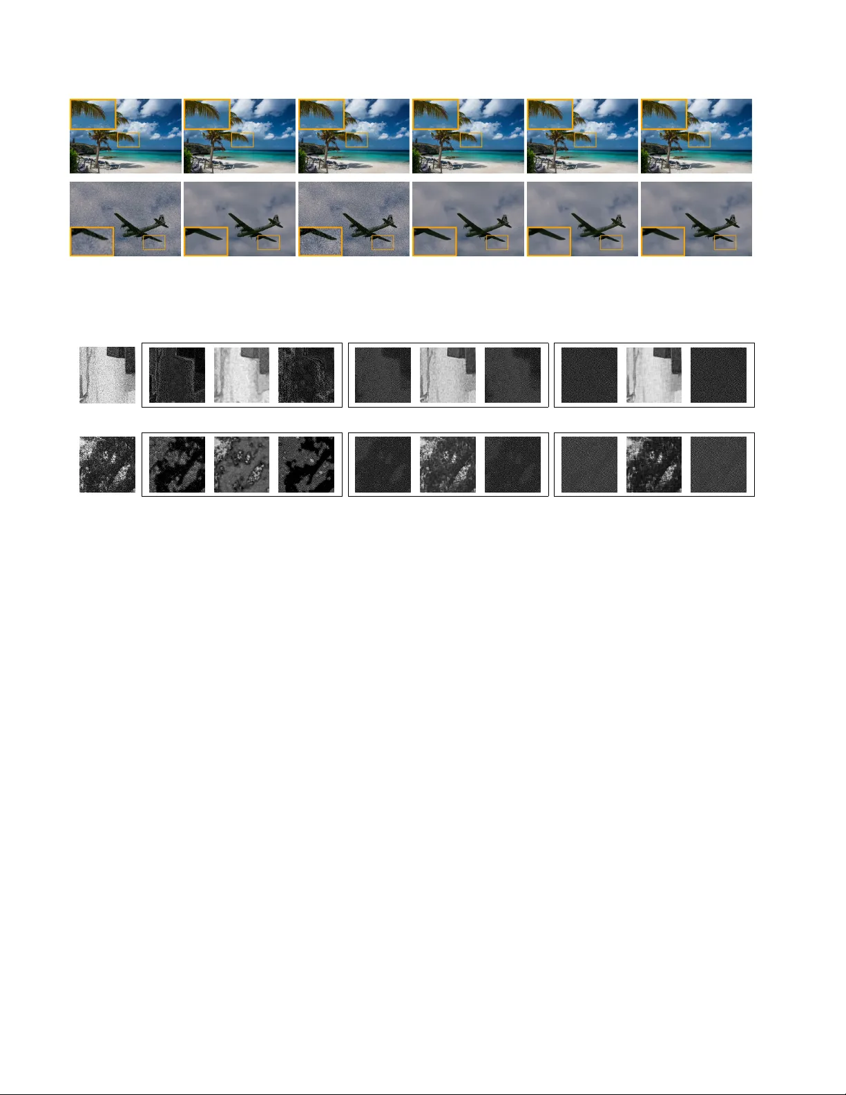
Original Paper
Loading high-quality paper...
Comments & Academic Discussion
Loading comments...
Leave a Comment