Constrained Attractor Selection Using Deep Reinforcement Learning

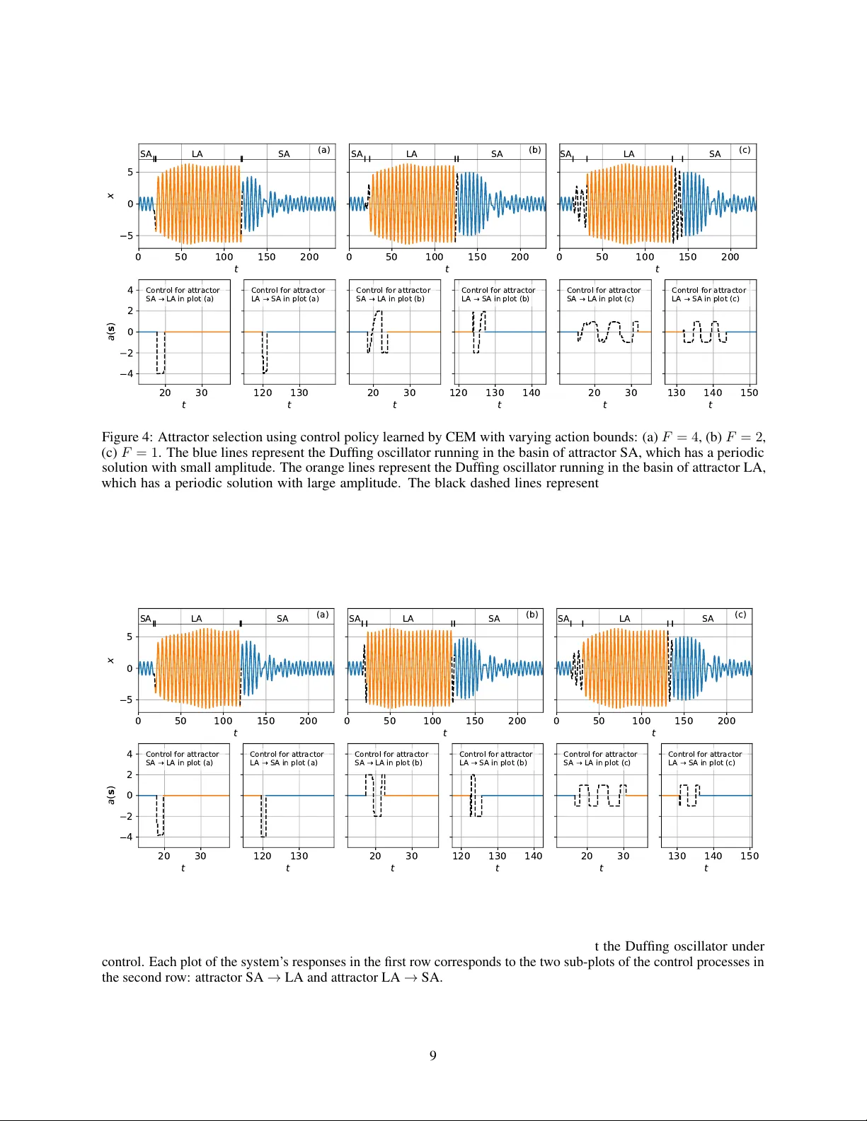
C O N S T R A I N E D A T T R A C T O R S E L E C T I O N U S I N G D E E P R E I N F O R C E M E N T L E A R N I N G A P R E P R I N T Xue-She W ang, James D. T ur ner & Brian P . Mann Dynamical Systems Research Laboratory Department of Mechanical Engineering & Materials Science Duke Uni versity Durham, NC 27708, USA xueshe.wang@duke.edu June 2, 2020 A B S T R AC T This paper describes an approach for attractor selection (or multi-stability control) in nonlinear dynamical systems with constrained actuation. Attractor selection is obtained using two dif ferent deep reinforcement learning methods: 1) the cross-entropy method (CEM) and 2) the deep deterministic policy gradient (DDPG) method. The framew ork and algorithms for applying these control methods are presented. Experiments were performed on a Duffing oscillator , as it is a classic nonlinear dynamical system with multiple attractors. Both methods achie ve attractor selection under v arious control constraints. While these methods hav e nearly identical success rates, the DDPG method has the advantages of a high learning rate, lo w performance v ariance, and a smooth control approach. This study demonstrates the ability of two reinforcement learning approaches to achiev e constrained attractor selection. K eywords Coexisting attractors · Attractor selection · Reinforcement learning · Machine learning · Nonlinear dynamical system 1 Introduction Coexisting solutions or stable attractors are a hallmark of nonlinear systems and appear in highly disparate scientific applications [ 1 , 2 , 3 , 4 , 5 , 6 , 7 , 8 ]. For these systems with multiple attractors, there often e xists a preferable solution and one or more less preferable, or potentially catastrophic, solutions [ 9 ]. For example, man y nonlinear energy harv esters hav e multiple attractors, each with dif ferent le vels of po wer output, among which the highest-power one is typically desired [ 10 , 11 , 12 ]. Another example is the coexistence of period-1 and period-2 rhythms in cardiac dynamics. Controlling the trajectory of the cardiac rhythm to period-1 is desirable to av oid arrhythmia [ 13 , 14 ]. Furthermore, coexisting solutions also appear in ecology and represent v arious degrees of ecosystem biodiv ersity [ 15 ], where a bio-manipulation scheme is needed to av oid certain detrimental en vironmental states [16]. These and other applications ha ve moti vated the de velopment of sev eral control methods to switch between attractors of nonlinear dynamical systems. Pulse control is one of the simplest methods; it applies a specific type of perturbation to direct a system’ s trajectory from one basin of attraction to another and waits until the trajectory settles do wn to the desired attractor [ 17 , 18 , 19 ]. T argeting algorithms, which were presented by Shinbrot et al. and modified by Macau et al., exploit the exponential sensitivity of basin boundaries in chaotic systems to small perturbations to direct the trajectory to a desired attractor in a short time [ 20 , 21 ]. Lai de veloped an algorithm to steer most trajectories to a desired attractor using small feedback control, which builds a hierarchy of paths tow ards the desirable attractor and then stabilizes a trajectory around one of the paths [ 22 ]. Besides switching between naturally stable attractors, one can also stabilize the unstable periodic orbits and switch between these stabilized attractors. Since the OGY method A P R E P R I N T - J U N E 2 , 2 0 2 0 was de vised by Ott, Grebogi, and Y orke in 1990 [ 23 ], numerous works ha ve b uilt upon this original idea and explored relev ant applications [24, 25, 26, 27, 28, 29]. Although these methods can work for certain categories of problems, the y are subject to at least one of the follo wing restrictions: (1) they only work for chaotic systems; (2) the y only w ork for autonomous systems; (3) the y need e xistence of unstable fixed points; (4) they cannot apply constraints to control; or (5) they cannot apply control optimization. Especially for the last two limitations, the compatibility with constrained optimal control is difficult to realize for most methods mentioned yet plays an important role in designing a real-world controller . For e xample, the limitations on the instantaneous po wer/force and total energy/impulse of a controller need be considered in practice. Another practical consideration is the optimization of total time and ener gy spent on the control process. Switching attractors using as little time or energy as possible is oftentimes required, especially when attempting to escape detrimental responses or using a finite energy supply . Fortunately , a technique that is compatible with a broader scope of nonlinear systems, Reinforcement Learning (RL), can be applied without the aforementioned restrictions. By learning action-decisions while optimizing the long-term consequences of actions, RL can be vie wed as an approach to optimal control of nonlinear systems [ 30 ]. V arious control constraints can also be applied by carefully defining a re ward function in RL [ 31 ]. Although several studies of attractor selection using RL were published decades ago [ 32 , 33 , 34 ], they dealt with only chaotic systems with unstable fixed points due to the limited choice of RL algorithms at the time. In recent years, a large number of adv anced RL algorithms ha ve been created to address complex control tasks. Most tasks with complicated dynamics have been implemented using the 3D ph ysics simulator MuJoCo [ 35 ], including control of Swimmer , Hopper , W alker [ 36 , 37 ], Half-Cheetah [ 38 ], Ant [ 39 ] and Humanoid [ 40 ] systems for balance maintenance and fast mo vement. Apart from simulated tasks, RL implementation in real-world applications includes motion planing of robotics [ 41 ], autonomous dri ving [ 42 ], and acti ve damping [ 43 ]. Furthermore, sev eral researchers hav e explored RL-based optimal control for gene regulatory networks (GRNs), with the goal of dri ving gene expression tow ards a desirable attractor while using a minimum number of interv entions [ 44 ]. For example, Sirin et al. applied the model-free batch RL Least-Squares Fitted Q Iteration (FQI) method to obtain a controller from data without e xplicitly modeling the GRN [ 45 ]. Imani et al. used RL with Gaussian processes to achiev e near-optimal infinite-horizon control of GRNs with uncertainty in both the interv entions and measurements [ 46 ]. Papagiannis et al. introduced a novel learning approach to GRN control using Double Deep Q Netw ork (Double DQN) with Prioritized Experience Replay (PER) and demonstrated successful results for larger GRNs than previous approaches [ 47 , 48 ]. Although these applications of RL for reaching GRNs’ desirable attractors are related to our goal of switching attractors in continuous nonlinear dynamical systems, they are limited to Random Boolean Networks (RBN), which ha ve discrete state and action spaces. A further in vestigation into generic nonlinear dynamical systems, where states and control inputs are oftentimes continuous, is therefore needed. This paper will apply two RL algorithms, the cross-entropy method (CEM) and deep deterministic policy gradi- ent (DDPG), to in vestigate the problem of attractor selection for a representati ve nonlinear dynamical system. 2 Reinf orcement Lear ning (RL) Framework In the RL framew ork shown in Fig. 1, an agent gains experience by making observations , taking actions and recei ving r ewar ds from an en vir onment , and then learns a policy from past experience to achie ve goals (usually maximized cumulativ e r ewar d ). T o implement RL for control of dynamical systems, RL can be modeled as a Markov Decision Process (MDP): 1. A set of en vironment states S and agent actions A . 2. P a ( s, s 0 ) = Pr ( s t +1 = s 0 | s t = s, a t = a ) is the probability of transition from state s at time t to state s 0 at time t + 1 with action a . 3. r a ( s, s 0 ) is the immediate rew ard after transition from s to s 0 with action a . A deterministic dynamical system under control is generally represented by the gov erning differential equation: ˙ x = f ( x, u, t ) , (1) where x is the system states, ˙ x is the states’ rate of change, and u is the control input. The governing equation can be inte grated ov er time to predict the system’ s future states giv en initial conditions; it plays the same role as the transition probability in MDP . This equiv alent interpretation of the gov erning equations and transition probability offers the opportunity to apply RL to control dynamical systems. The en vironment in RL can be either the system’ s gov erning equation if RL is implemented in simulation, or the e xperimental setup interacting with the real world if RL 2 A P R E P R I N T - J U N E 2 , 2 0 2 0 Figure 1: The typical frame work of Reinforcement Learning. An agent has two tasks in each iteration: (1) taking an action based on the observation from en vironment and the current polic y; (2) updating the current policy based on the immediate rew ard from en vironment and the estimated future rew ards. 0.4 0.6 0.8 1 1.2 1.4 1.6 1.8 2 0 1 2 3 4 5 6 7 (a) -6 -4 -2 0 2 4 6 -8 -6 -4 -2 0 2 4 6 8 (b) attractor LA attractor SA attractor LA attractor SA Figure 2: Coexisting attractors for the hardening Duf fing oscillator: ¨ x + 0 . 1 ˙ x + x + 0 . 04 x 3 = cos ω t . (a) Frequency responses. (b) Phase portrait of coexisting solutions when ω = 1 . 4 . W ithin a specific frequency range, periodic solutions coexist in (a), including tw o stable solutions (green solid lines) and an unstable solution (red dashed line) in-between. The stable solutions correspond to an attractor with small amplitude (SA) and one with large amplitude (LA). The dotted line in (b) is a trajectory of switching attractor SA → LA using the control method introduced in this paper . is implemented for a physical system. Instead of the con ventional notation of states x and control input u in control theory , research in RL uses s and a to represent states and actions respectively . These RL-style notations are used throughout the remainder of this article. This paper implements RL algorithms to realize attractor selection (control of multi-stability) for nonlinear dynamical systems with constrained actuation. As a representati ve system possessing multiple attractors, the Duf fing oscillator was chosen to demonstrate implementation details. En vironment . A harmonically forced Duf fing oscillator , which can be described by the equation ¨ x + δ ˙ x + αx + β x 3 = Γ cos ω t , provides a familiar example for e xploring the potential of RL for attractor selection. Fig. 2 shows an e xample of a hardening ( α > 0 , β > 0 ) frequency response. For certain ranges of the parameters, the frequency response is a multiple-valued function of ω , which represents multiple coexisting steady-state oscillations at a given forcing 3 A P R E P R I N T - J U N E 2 , 2 0 2 0 frequency . W ith a long-run time e v olution, the oscillation of the unstable solution cannot be maintained due to inevitable small perturbations. The system will alw ays ev entually settle into one of the stable steady-state responses of the system, which are therefore considered “attractors”. Our objecti ve is to apply control to the Duffing oscillator to make it switch between the two attractors using constrained actuation. T o provide actuation for attractor selection, an additional term a ( s ) , is introduced into the go verning equation: ¨ x + δ ˙ x + αx + β x 3 = Γ cos ( ω t + φ 0 ) + a ( s ) . (2) where a ( s ) is the actuation which depends on the system’ s states s . For example, if the Duffing oscillator is a mass–spring–damper system, a ( s ) represents a force. Action . Aligned with the practical consideration that an actuation is commonly constrained, the action term can be written as a ( s ) := F π θ ( s ) , where F is the action bound which denotes the maximum absolute v alue of the actuation, and π θ ( s ) is the control polic y . π θ ( s ) is designed to be a function parameterized by θ , which has an input of the Duf fing oscillator’ s states s , and an output of an actuation scaling v alue between − 1 and 1 . Our objective is achie ved by finding qualified parameters θ that cause the desired attractor to be selected. State & Observation . The Duffing oscillator is dri ven by a time-v arying force Γ cos ω t ; thus, the state should consist of position x , velocity ˙ x , and time t . Giv en that Γ cos ω t is a sinusoidal function with a phase periodically increasing from 0 to 2 π , time can be replaced by phase for a simpler state expression. The system’ s state can therefore be written as s := [ x, ˙ x, φ ] , where φ is equal to ω t modulo 2 π . For the sake of simplicity , we have assumed that no observ ation noise was introduced and the states were fully observ able by the agent. Reward . A well-trained policy should use a minimized control ef fort to reach the tar get attractor; thus the reward function, which is determined by state s t and action a t , should inform the cost of the action taken and whether the Duffing oscillator reaches the target attractor . The action cost is defined as the impulse gi ven by the actuation, | a t | ∆ t , where ∆ t is the time step size for control. The en vironment estimates whether the tar get attractor will be reached by ev aluating the ne xt state s t +1 . A constant reward of r end is giv en only if the target attractor will be reached. For estimating whether the target attractor will be reached, one could observ e whether s t +1 is in the “basin of attraction” of the target attractor . Basins of attraction (BoA) are the sets of initial states leading to their corresponding attractors as time e volves (see Fig. 3). Once the target BoA is reached, the system will automatically settle into the desired stable trajectory without further actuation. Therefore, the reward function can be written as: r ( s t , a t ) = −| a t | ∆ t +  r end , if s t +1 reaches target BoA 0 , otherwise (3) BoA Classification . Determining whether a state is in the target BoA is non-trivial. For an instantaneous state s t = [ x t , ˙ x t , φ t ] , we could set a ( s ) = 0 in Eq. (2) and integrate it with the initial condition [ x 0 , ˙ x 0 , φ 0 ] = s t . Integrating for a sufficiently long time should give a steady-state response, whose amplitude can be ev aluated to determine the attractor . Howe v er , this prediction is needed for each time step of the reinforcement learning process, and the integration time should be suf ficiently long to obtain steady-state responses; thus this approach results in e xpensiv e computational workload and a slo w learning process. As a result, a more ef ficient method was needed for determining which attractor corresponded to the system’ s state [49]. Since the number of attractors is finite, the attractor prediction problem can be considered a classification problem, where the input is the system’ s state and the output is the attractor label. Giv en that the boundary of the basins is nonlinear as sho wn in Fig. 3, the classification method of support vector machines (SVM) with Gaussian k ernel was selected for the Duf fing oscillator . For other nonlinear dynamical systems, logistic re gression is recommended for a linear boundary of basins, and a neural netw ork is recommended for a lar ge number of attractors. The training data was created by sampling states uniformly on the domain of three state v ariables, and the attractor label for each state was determined by the method mentioned abo ve: ev aluating future responses with long-term inte gration of governing equation. Generally speaking, this method transfers the recurring cost of integration during the reinforcement learning process to a one-time cost before the learning process begins. Collecting and labeling the data for training the classifier can be time consuming, b ut once the classifier is well-trained, the time for predicting the final attractor can be ne gligibly small. 3 Algorithms This section describes two RL algorithms for attractor selection, the cross-entropy method (CEM) and deep deterministic policy gradient (DDPG). These two methods were selected for their ability to operate over continuous action and state spaces [50]. This section will first explain a fe w important terms before describing the specifics of each algorithm. 4 A P R E P R I N T - J U N E 2 , 2 0 2 0 Figure 3: Basins of attraction (BoA) determined by the Duf fing oscillator’ s state v ariables, [ x, ˙ x, φ ] . Each point in the BoA represents an initial condition which drives the system to a certain attractor without control. The orange solid line and the shaded areas are the lar ge-amplitude attractor and its corresponding BoA, respecti vely . The blue dashed line and the blank areas are the small-amplitude attractor and its corresponding BoA, respectiv ely . Phase 1 : the phase where the system is free of control, i.e., a ( s ) = 0 . The system is gi ven a random initial condition at the beginning of Phase 1, waits for dissipation of the transient, and settles down on the initial attractor at the end of Phase 1. Phase 2 : the phase following Phase 1; the system is under control. Phase 2 starts with the system running in the initial attractor , and ends with either reaching the target BoA or e xceeding the time limit. T r ajectory : the system’ s time series for Phase 2. CEM uses trajectories of state-action pairs [ s t , a t ] , while DDPG uses trajectories of transitions [ s t , a t , r t , s t +1 ] . The data of trajectories are stored in a replay buf fer . Replay Buffer : an implementation of experience replay [51], which randomly selects previously e xperienced samples to update a control policy . Experience replay stabilizes the RL learning process and reduces the amount of experience required to learn [52]. The entire process for learning a control polic y can be summarized as iterati ve episodes. In each episode, the system runs through Phase 1 and Phase 2 in turn and the control policy is improv ed using the data of trajectories stored in the replay buf fer . CEM and DDPG are dif ferent methods for updating the control policy . The cross-entropy method (CEM) was pioneered as a Monte Carlo method for importance sampling, estimating probabilities of rare ev ents in stochastic networks [ 53 , 54 ]. The CEM in volves an iterati ve procedure of two steps: (1) generate a random data sample according to a specified mechanism; and (2) update the parameters of the random mechanism based on the data to produce a “better” sample in the next iteration [55]. In recent decades, an increasing number of applications of the CEM hav e been found for reinforcement learning [ 56 , 57, 58]. CEM-based RL can be represented as an iterativ e algorithm [59]: π i +1 ( s ) = arg min π i +1 − E z ∼ π i ( s ) [ R ( z ) > ρ i ] log π i +1 ( s ) , (4) where R ( z ) = X t r ( s t , a t | z ∼ π i ( s )) . (5) R ( z ) is the cumulati ve re ward of a single time series trajectory generated by the current control polic y π i ( s ) , and ρ i is the re ward threshold abo ve which the trajectories are considered successful samples. This iteration minimizes the negati ve log likelihood (i.e., maximizes the log likelihood) of the most successful trajectories to impro ve the current policy . 5 A P R E P R I N T - J U N E 2 , 2 0 2 0 In our scenario where the control policy π ( s ) is a neural network parameterized by θ , the CEM iteration can also be written as: θ i +1 = arg min θ P j L ( a j , F π θ i ( s j )) 1 A ( s j ) P j 1 A ( s j ) , (6) where A = { s j : s j ∈ T k and R T k > ρ k } . (7) Giv en a state s j picked from the replay b uf fer , L ( · , · ) is the loss function of the dif ference between its corresponding action value from past experience a j , and the action value predicted by the current policy F π θ i . The indicator function 1 A ( s j ) has the v alue 1 when a state s j belongs to a successful trajectory T k (i.e., the cumulati ve rew ard of the trajectory R T k is greater than the a threshold ρ k ), and has the v alue 0 otherwise. The detailed CEM algorithm designed for attractor selection is presented in the experiment section. Deep Deterministic P olicy Gradient (DDPG) is a RL algorithm that can operate o ver continuous state and action spaces [ 60 ]. The goal of DDPG is to learn a polic y which maximizes the expected return J = E r i ,s i ,a i [ R t =1 ] , where the return from a state is defined as the sum of discounted future rew ards R t = P T i = t γ i − t r ( s i , a i ) with a discount factor γ ∈ [0 , 1] . An action-value function, also kno wn as a “critic” or “Q-v alue” in DDPG, is used to describe the expected return after taking an action a t in state s t : Q ( s t , a t ) = E r i > t ,s i>t ,a i>t [ R t | s t , a t ] . (8) DDPG uses a neural network parameterized by ψ as a function appropriator of the critic Q ( s, a ) , and updates this critic by minimizing the loss function of the dif ference between the “true” Q-v alue Q ( s t , a t ) and the “estimated” Q-v alue y t : L ( ψ ) = E s t ,a t ,r t h ( Q ( s t , a t | ψ ) − y t ) 2 i , (9) where y t = r ( s t , a t ) + γ Q ( s t +1 , π ( s t +1 ) t | ψ ) . (10) Apart from the “critic”, DDPG also maintains an “actor” function to map states to a specific action, which is essentially our policy function π ( s ) . DDPG uses another neural network parameterized by θ as a function approximator of the actor π ( s ) , and updates this actor using the gradient of the expected return J with respect to the actor parameters θ : ∇ θ J ≈ E s t  ∇ a Q ψ ( s, a ) | s = s t ,a = π ( s t ) ∇ θ π θ ( s ) | s = s t  . (11) In order to enhance the stability of learning, DDPG is inspired by the success of Deep Q Network (DQN) [ 61 , 52 ] and uses a “replay b uffer” and separate “tar get networks” for calculating the estimated Q-value y t in Eq. (10) . The replay buf fer stores transitions [ s t , a t , r t , s t +1 ] from experienced trajectories. The actor π ( s ) and critic Q ( s, a ) are updated by randomly sampling a minibatch from the buf fer , allo wing the RL algorithm to benefit from stably learning across uncorrelated transitions. The target networks are copies of actor and critic networks, π 0 θ 0 ( s ) and Q 0 ψ 0 ( s, a ) respectiv ely , that are used for calculating the estimated Q-v alue y t . The parameters of these target networks are updated by slo wly tracking the learned networks π θ ( s ) and Q ψ ( s, a ) : ψ 0 ← τ ψ + (1 − τ ) ψ 0 , θ 0 ← τ θ + (1 − τ ) θ 0 , (12) where 0 < τ  1 . This soft update constrains the estimated Q-v alue y t to change slo wly , thus greatly enhancing the stability of learning. The detailed DDPG algorithm designed for attractor selection is presented in the experiment section. One major difference between CEM and DDPG is the usage of the policy gradient ∇ θ J . DDPG computes the gradient for policy updates in Eq. (11) while CEM is a gradient-free algorithm. Another difference lies in their approach to using stored experience in the replay b uffer . CEM impro ves the policy after collecting ne w trajectories of data, while DDPG continuously improv es the policy at each time step as it explores the en vironment [50]. 4 Experiment This section presents the details of the experiment performing attractor selection for the Duffing oscillator using CEM and DDPG. 6 A P R E P R I N T - J U N E 2 , 2 0 2 0 T able 1: Algorithm: Cross-Entropy Method (CEM) for Attractor Selection 1 Randomly initialize policy network π θ ( s ) with weight θ 2 Set the initial condition of the Duffing equation s 0 = [ x 0 , ˙ x 0 , φ 0 ] 3 Set time of Phase 1 and Phase 2, T 1 and T 2 4 Set best sample proportion, p ∈ [0 , 1] 5 for episode = 1 : M do 6 Initialize an empty replay buf fer B 7 for sample = 1 : N do 8 Initialize an empty buf fer ˜ B 9 Initialize a random process N for action exploration 10 Initialize trajectory rew ard, R = 0 11 Add noise to time of Phase 1, T 1 0 = T 1 + random (0 , 2 π/ω ) 12 Integrate Eq. (2) for t ∈  0 , T 1 0  with a ( s ) = 0 Phase 1 13 for t = T 1 0 : T 1 0 + T 2 do Phase 2 14 Observe current state, s t = [ x t , ˙ x t , φ t ] 15 Evaluate action a t ( s t ) = F π θ ( s t ) + N t , according to the current policy and e xploration noise 16 Step into the next state s t +1 , by integrating Eq. (2) for ∆ t 17 Update trajectory rew ard R ← R + r ( s t , a t ) , according to Eq. (3) 18 Store state-action pair [ s t , a t ] in ˜ B 19 Evaluate the basin of attraction for s t +1 20 if the target attractor’ s basin is reached: 21 Label each state-action pair [ s t , a t ] in ˜ B with trajectory rew ard R , and append them to B 22 break 23 end for 24 end for 25 Choose the a minibatch of the elite p proportion of ( s, a ) in B with the largest re ward R 26 Update policy π θ ( s ) by minimizing the loss, L = 1 Minibatch Size P i ( F π θ ( s i ) − a i ) 2 27 end for The governing equation for the Duf fing oscillator is given by Eq. (2) , where δ = 0 . 1 , α = 1 , β = 0 . 04 , Γ = 1 and ω = 1 . 4 . The Duffing equation is integrated using scipy .integrate.odeint() in Python with a time step of 0.01. The time step for control is 0.25, and reaching the target BoA will add a re ward r end = 100 . Therefore, the re ward function Eq. (3) can be written as: r ( s t , a t ) =  100 − 0 . 25 | a t | , if s t +1 reaches target BoA, − 0 . 25 | a t | , otherwise. (13) For the estimation of BoA, the SVM classifier with radial basis function (RBF) kernel w as trained using a 50 × 50 × 50 grid of initial conditions, with x ∈ [ − 10 , 10] , ˙ x ∈ [ − 15 , 15] and φ ∈ [0 , 2 π ] . The detailed attractor selection algorithm using CEM can be found in T ab . 1. In line 11, the time of Phase 1 is perturbed by adding a random value between 0 and 2 π /ω (a forcing period). This noise provides di versity of the system’ s states at the be ginning of Phase 2, which enhances generality and helps pre vent over -fitting of the control policy network π θ ( s ) . The policy network π θ ( s ) has two fully connected hidden layers, each of which has 64 units and an acti v ation function of ReLU [ 62 ]. The final output layer is a tanh layer to bound the actions. Adam optimizer [ 63 ] with a learning rate of 10 − 3 and a minibatch size of 128 was used for learning the neural network parameters. For the system’ s settling down in Phase 1 we used T 1 = 15 , and for constraining the time length of control we used T 2 = 20 . In each training episode, state-action pairs from 30 trajectory samples were stored in the replay b uffer ( N = 30 ), and those with reward in the top 80% were selected for training the network ( p = 0 . 8 ). The detailed attractor selection algorithm using DDPG can be found in T ab . 2. Apart from the “actor” network π θ ( s ) which is same as the policy netw ork in the CEM, the DDPG introduces an additional “critic” network Q ψ ( s, a ) . This Q network is designed to be a neural network parameterized by ψ , which has the system’ s state and corresponding action as inputs, and a scalar as the output. As in the algorithm using CEM, the state diversity is promoted by introducing noise to the time of Phase 1 in line 9. Both the actor network π θ ( s ) and the critic network Q ψ ( s, a ) hav e two hidden layers, each of which has 128 units and an activ ation function of ReLU [ 62 ]. For the actor network, the final output layer is a tanh layer to bound the actions. F or the critic network, the input layer consists of only the state s , while the action a is included in the 2nd hidden layer . Adam optimizer [ 63 ] was used to learn the neural network parameters with 7 A P R E P R I N T - J U N E 2 , 2 0 2 0 T able 2: Algorithm: Deep Deterministic Policy Gradient (DDPG) for Attractor Selection 1 Randomly initialize actor network π θ ( s ) and critic network Q ψ ( s, a ) with weights θ and ψ 2 Initialize target netw ork π 0 θ 0 ( s ) and Q 0 ψ 0 ( s, a ) with weights θ 0 ← θ , ψ 0 ← ψ 3 Set the initial condition of the Duffing equation s 0 = [ x 0 , ˙ x 0 , φ 0 ] 4 Set discount factor γ , and soft update factor τ 5 Set time of Phase 1 and Phase 2, T 1 and T 2 6 Initialize replay buf fer B 7 for episode = 1 : M do 8 Initialize a random process N for action exploration 9 Add noise to time of Phase 1, T 1 0 = T 1 + random (0 , 2 π/ω ) 10 Integrate Eq. (2) for t ∈  0 , T 1 0  with a ( s ) = 0 Phase 1 11 for t = T 1 0 : T 1 0 + T 2 do Phase 2 12 Observe current state, s t = [ x t , ˙ x t , φ t ] 13 Evaluate action a t ( s t ) = F π θ ( s t ) + N t , according to the current policy and e xploration noise 14 Step into the next state s t +1 , by integrating Eq. (2) for ∆ t 15 Evaluate re ward r t ( s t , a t ) , according to Eq. (3) 16 Store transition [ s t , a t , r t , s t +1 ] in B 17 Sample a random minibatch of N transitions [ s i , a i , r i , s i +1 ] from B 18 Set y i = r i + γ Q 0 ψ 0 ( s i +1 , F π 0 θ 0 ( s i +1 )) 19 Update the critic network by minimizing the loss: L = 1 N P i ( y i − Q ψ ( s i , a i )) 2 20 Update the actor network using the sampled policy gradient: ∇ θ J ≈ 1 N P i ∇ a Q ψ ( s, a ) | s = s i ,a = F π θ ( s i ) ∇ θ π θ ( s ) | s = s i 21 Update the target netw orks: ψ 0 ← τ ψ + (1 − τ ) ψ 0 , θ 0 ← τ θ + (1 − τ ) θ 0 22 if the target attractor’ s basin is reached in s t +1 : break 23 end for 24 end for a learning rate of τ θ = 10 − 4 and τ ψ = 10 − 3 for the actor and critic respecti v ely . For the update of the critic network we used a discount factor of γ = 0 . 9 . For the soft update of the target network π 0 θ 0 ( s ) and Q 0 ψ 0 ( s, a ) by Polyak A veraging, we used τ = 0 . 1 . For the system’ s settling down in Phase 1 we used T 1 = 15 , and for constraining the time length of control we used T 2 = 20 . The replay buf fer had a size of 10 6 . In each episode, the minibatch of transitions sampled from the replay buf fer had a size of N = 64 . T o test the CEM and DDPG algorithms, constraints were constructed with v arying le vels of difficulty , i.e., dif ferent action bounds F . Recall that the control term in Eq. (2) can be written as a ( s ) = F π θ ( s ) , which is bounded between − F and F . It’ s also worth noting that each policy only controls a one-way trip of attractor switching. For the example of a Duffing oscillator with two attractors, one control policy is needed for transitioning from the small-amplitude attractor to the large-amplitude one, and another control polic y is needed for the rev erse direction. 5 Results Fig. 4 and Fig. 5 sho w the time series of attractor selection using the control polic y learned by the CEM and DDPG algorithms, respectiv ely . For simplicity , the attractor with a small amplitude of steady-state response is named “SA ” while that with a large amplitude is named “LA ”. For all six test cases in Fig. 4 and Fig. 5, the Duf fing oscillator starts near the SA solution, then switches from SA to LA, and finally switches backwards from LA to SA. Compared with the short time length for control (region of black lines), the attractor selection spends more time w aiting for dissipation of the transient process, where the system is automatically approaching the target attractor under no control. This observ ation shows a smart and ef ficient strategy the control policy has learned: instead of dri ving the system precisely to the state set of the tar get attractor , it just driv es the system to the attractor’ s basin, where the system might be far a way from the target attractor initially b ut will reach it without further control effort as time e v olves. 8 A P R E P R I N T - J U N E 2 , 2 0 2 0 0 50 100 150 200 t 5 0 5 x (a) SA LA SA 20 30 t 4 2 0 2 4 a ( s ) Control for attractor SA LA in plot (a) 120 130 t Control for attractor LA SA in plot (a) 0 50 100 150 200 t (b) SA LA SA 20 30 t Control for attractor SA LA in plot (b) 120 130 140 t Control for attractor LA SA in plot (b) 0 50 100 150 200 t (c) SA LA SA 20 30 t Control for attractor SA LA in plot (c) 130 140 150 t Control for attractor LA SA in plot (c) Figure 4: Attractor selection using control policy learned by CEM with v arying action bounds: (a) F = 4 , (b) F = 2 , (c) F = 1 . The blue lines represent the Duf fing oscillator running in the basin of attractor SA, which has a periodic solution with small amplitude. The orange lines represent the Duf fing oscillator running in the basin of attractor LA, which has a periodic solution with large amplitude. The black dashed lines represent the Duf fing oscillator under control. Each plot of the system’ s responses in the first ro w corresponds to the two sub-plots of the control processes in the second row: attractor SA → LA and attractor LA → SA. 0 50 100 150 200 t 5 0 5 x (a) SA LA SA 20 30 t 4 2 0 2 4 a ( s ) Control for attractor SA LA in plot (a) 120 130 t Control for attractor LA SA in plot (a) 0 50 100 150 200 t (b) SA LA SA 20 30 t Control for attractor SA LA in plot (b) 120 130 140 t Control for attractor LA SA in plot (b) 0 50 100 150 200 t (c) SA LA SA 20 30 t Control for attractor SA LA in plot (c) 130 140 150 t Control for attractor LA SA in plot (c) Figure 5: Attractor selection using control polic y learned by DDPG with varying action bounds: (a) F = 4 , (b) F = 2 , (c) F = 1 . The blue lines represent the Duf fing oscillator running in the basin of attractor SA, which has a periodic solution with small amplitude. The orange lines represent the Duf fing oscillator running in the basin of attractor LA, which has a periodic solution with large amplitude. The black dashed lines represent the Duf fing oscillator under control. Each plot of the system’ s responses in the first ro w corresponds to the two sub-plots of the control processes in the second row: attractor SA → LA and attractor LA → SA. 9 A P R E P R I N T - J U N E 2 , 2 0 2 0 0.00 0.25 0.50 0.75 1.00 Success Rate (a) F = 4 F = 2 F = 1 CEM 0 3000 6000 9000 Samples 0 100 200 300 Episode 100 50 0 50 100 Expected Reward (c) F = 4 F = 2 F = 1 (b) F = 4 F = 2 F = 1 DDPG 0 100 200 300 Samples 0 100 200 300 Episode (d) F = 4 F = 2 F = 1 Figure 6: The control policy performance curve for the success rate of reaching tar get attractor using (a) CEM and (b) DDPG, and the expected accumulated re ward of a control process using (c) CEM and (d) DDPG. The v arying action bound of 4, 2, and 1 are represented by the blue, orange, and green lines respecti vely . The gray areas in plot (c) and (d) represent standard deviation of the accumulated re wards. One can also observ e that a smaller action bound results in a longer time length of control for both CEM and DDPG algorithms. It can be qualitativ ely explained by the ener gy threshold for jumping from one attractor to another . The energy pro vided by the actuation should be accumulated beyond the ener gy threshold to push the system away from one attractor . A smaller action bound therefore leads to longer time for the ener gy accumulation. Another observation is that the system quickly approaches near LA when starting from SA, while it takes more time to approach near SA when starting from LA. This can be e xplained using the unstable solution of the Duf fing equation which is represented as the red dashed circle in Fig. 2 (b). This circle can be considered the boundary between the basins of two attractors, across which the system jumps from one attractor to another . This boundary is close to LA, which means that the system will be near LA immediately after going across the boundary from SA. In contrast, SA is far from the boundary; therefore, a longer time is needed to reach near SA after going across the boundary from LA. The attractors’ distances from the unstable solution also indicate their robustness and lik elihood of occurrence. In this Duffing oscillator , SA is more rob ust and more likely to occur than LA. The successful switching from a more likely attractor (such as SA) to a less likely attractor (such as LA), which is difficult for traditional control methods, is another advantage of the proposed RL-based methods. Although the CEM and DDPG algorithms both achie ve attractor selection with various action bounds, DDPG has advantages of providing smooth actuations. From the comparison of the actuation F π θ ( s ) between Fig. 4 and Fig. 5, the actuation from CEM shows more jagged motion than that from DDPG especially for the small action bound. More advantages of DDPG o ver CEM can be observed in Fig. 6, which compares the trend of their policies’ success rate and expected re ward during learning process. In each learning episode, 100 samples with random initial states were used to ev aluate the control policy’ s success rate of reaching the tar get attractor and the mean and standard de viation of the samples’ accumulated rew ard. For faster con ver gence, the policy trained for a tighter action bound was initialized with the parameters of a well-trained polic y for a more generous action bound. In other words, instead of learning from nothing, a policy learned to solv e a hard problem from the experience of solving an easy one. The “untrained” polic y for the action bound of 2 was initialized with the parameters of the “trained” polic y for the action bound of 4, and so on. Therefore in Fig. 6, the action bound decreases as the learning episode increases. The success rates and expected rewards were equally high for both CEM and DDPG at the end of the learning for each action bound (episode = 100, 200, 300), but DDPG con ver ged faster , especially for the action bound of 1. This advantage of DDPG can be observed from the performance curve which e volv es with “episode” in Fig. 6, b ut DDPG is ev en better than this considering that it spends much less time on each episode than CEM. As shown in the T able 1, CEM needs N samples of trajectories for updating the policy in each episode, while DDPG (see T able 2) collects only the sample of a single trajectory . The real learning speed can therefore be reflected by the total “samples” generated 10 A P R E P R I N T - J U N E 2 , 2 0 2 0 instead of “episode”. Fig. 6 shows the DDPG’ s advantage of learning speed and data ef ficiency by providing an additional horizontal axis for the number of samples, where CEM generates 30 samples per episode while DDPG generates only 1 sample per episode. Parallel computing can be used for helping CEM narro w the gap, b ut generally DDPG has a natural advantage of learning speed. Furthermore, after the CEM learned an optimal policy , it often degenerated to a sub-optimal policy , which can be observed from the small perturbation around episode 150 and the significant oscillation throughout episode 200–300 in Fig. 6 (b,d). In contrast, DDPG sho ws a lo wer variance of the policy performance after an optimal policy has been learned, which can be observed from the flat line in episode 100–200 and the comparativ ely small perturbation in episode 200–300. 6 Conclusion This work applies adv anced reinforcement learning (RL) methods to the control problem of attractor selection, resulting in algorithms that switch between coexisting attractors of a nonlinear dynamical system using constrained actuation. A control framew ork was presented combining attractor selection and general RL methods. T wo specific algorithms were designed based on the cross-entropy method (CEM) and deep deterministic policy gradient (DDPG). The Duffing oscillator , which is a classic nonlinear dynamical system with multiple coexisting attractors, was selected to demonstrate the control design and sho w the performance of the control policy learned by CEM and DDPG. Both methods achie ved attractor selection under v arious constraints on actuation. They had equally high success rates, b ut DDPG had advantages of smooth control, high learning speed, and lo w performance v ariance. The RL-based attractor selection is model-free and thus needs no prior knowledge on the system model. This provides broad applicability since precise mathematical models for man y real-world systems are often una vailable due to their highly nonlinear features or high noise lev el. Additionally , the control constraints can be easily customized for a wide variety of problems. Apart from constraining the maximum actuation in the Duf fing oscillator example, the system’ s position can be constrained in case of working in a limited space, the system’ s velocity can be constrained if there exists a hardware requirement of speed range, and the constraints themselv es can e ven be time-v arying. V arious constraints can be realized by carefully designing the action term and rew ard function. Future work needs to extend our in vestigations in three key directions. First, although the proposed approach is model-free and does not require a priori knowledge of the system dynamics when training the control policy , obtaining the basins of attraction (BoAs) might still require prior kno wledge of the system’ s equilibria and stability behavior as deriv ed from the governing equation. In order to entirely get rid of this model dependence, a data-driv en approach to automatically finding coe xisting attractors based on simulation or experimental data will be needed. Second, the quantity of samples for training a qualified BoA classifier needs to be reduced. As mentioned in the experiment section, the classifier w as trained using a 50 × 50 × 50 grid of 3-dimensional initial conditions. Each of 125 , 000 samples was obtained by running a simulation and e valuating its final state. A lar ge number of training samples will become a huge burden when (1) simulations are computationally e xpensiv e, (2) samples are collected from e xperiment, or (3) the dimension of initial conditions is high. A more data-ef ficient sampling method is therefore needed. Third, we would like to reiterate that the model-free approach proposed in this paper only indicates that a model is unnecessary for learning a control polic y , but does not mean the model is useless. If the approach is implemented in real-world experiments which are much more costly than simulations, a more ef ficient way is to first find a sub-optimal control policy in simulation and then “transfer” the pre-trained policy to the experiments for further optimization. This process is called “transfer learning”, where the heavy-learning workload in experiments is shared with simulations, and the simulation-based RL will need a model as its en vironment. More studies implementing the attractor selection approach based on real-world experiments and transfer learning are certainly w orthy topics for further in vestigations. This study demonstrated two reinforcement learning approaches for constrained attractor selection. These approaches make it possible to switch between attractors without the limitations of prior methods in the literature. By optimizing the policy subject to realistic constraints, the y are applicable to a wide variety of practical problems. References [1] John Michael T utill Thompson and H Bruce Ste wart. Nonlinear dynamics and chaos . John W iley & Sons, 2002. [2] E. Brun, B. Derighetti, D. Meier , R. Holzner , and M. Rav ani. Observation of order and chaos in a nuclear spin–flip laser . J. Opt. Soc. Am. B , 2(1):156–167, Jan 1985. [3] J Maurer and A Libchaber . Effect of the prandtl number on the onset of turb ulence in liquid 4he. Journal de Physique lettr es , 41(21):515–518, 1980. 11 A P R E P R I N T - J U N E 2 , 2 0 2 0 [4] Robert M May . Thresholds and breakpoints in ecosystems with a multiplicity of stable states. Natur e , 269(5628):471, 1977. [5] JL Hudson and JC Mankin. Chaos in the belousov–zhabotinskii reaction. The J ournal of Chemical Physics , 74(11):6171–6177, 1981. [6] Xue-She W ang, Michael J. Mazzoleni, and Brian P . Mann. Dynamics of unforced and v ertically forced rocking elliptical and semi-elliptical disks. Journal of Sound and V ibration , 417:341 – 358, 2018. [7] Xue-She W ang and Brian P . Mann. Nonlinear dynamics of a non-contact translational-to-rotational magnetic transmission. Journal of Sound and V ibration , 459:114861, 2019. [8] Xue-She W ang and Brian P . Mann. Dynamics of a magnetically excited rotational system. In Gaetan K erschen, M. R. W . Brake, and Ludovic Renson, editors, Nonlinear Structures and Systems, V olume 1 , pages 99–102, Cham, 2020. Springer International Publishing. [9] Alexander N. Pisarchik and Ulrike Feudel. Control of multistability . Physics Reports , 540(4):167 – 218, 2014. Control of multistability . [10] B.P . Mann and N.D. Sims. Energy harvesting from the nonlinear oscillations of magnetic le vitation. Journal of Sound and V ibration , 319(1):515 – 530, 2009. [11] Samuel C. Stanton, Clark C. McGehee, and Brian P . Mann. Nonlinear dynamics for broadband ener gy harvesting: In vestigation of a bistable piezoelectric inertial generator . Physica D: Nonlinear Phenomena , 239(10):640 – 653, 2010. [12] Samuel C Stanton, Clark C McGehee, and Brian P Mann. Reversible hysteresis for broadband magnetopiezoelastic energy harv esting. Applied Physics Letters , 95(17):174103, 2009. [13] Richard P Kline and B Mitchell Bak er . A dynamical systems approach to membrane phenomena underlying cardiac arrhythmias. International Journal of Bifur cation and Chaos , 5(01):75–88, 1995. [14] Ali R Y ehia, Dominique Jeandupeux, Francisco Alonso, and Michael R Guev ara. Hysteresis and bistability in the direct transition from 1: 1 to 2: 1 rhythm in periodically dri ven single v entricular cells. Chaos: An Inter disciplinary Journal of Nonlinear Science , 9(4):916–931, 1999. [15] Marten Scheffer , Stev e Carpenter , Jonathan A Fole y , Carl Folke, and Brian W alk er . Catastrophic shifts in ecosystems. Nature , 413(6856):591, 2001. [16] Egbert H V an Nes and Marten Scheffer . Slow recovery from perturbations as a generic indicator of a nearby catastrophic shift. The American Naturalist , 169(6):738–747, 2007. [17] Kunihik o Kaneko. Chaotic b ut regular posi-ne ga switch among coded attractors by cluster-size v ariation. Physical Revie w Letters , 63(3):219, 1989. [18] Kunihiko Kaneko. Clustering, coding, switching, hierarchical ordering, and control in a network of chaotic elements. Physica D: Nonlinear Phenomena , 41(2):137 – 172, 1990. [19] AM Samson, SI T urov ets, VN Chizhevsk y , and VV Churakov . Nonlinear dynamics of a loss-switched co2 laser . Sov . Phys. JETP , 74(4):628–639, 1992. [20] T roy Shinbrot, Edward Ott, Celso Grebogi, and James A Y orke. Using chaos to direct trajectories to targets. Physical Revie w Letters , 65(26):3215, 1990. [21] Elbert E. N. Macau and Celso Grebogi. Dri ving trajectories in complex systems. Phys. Rev . E , 59:4062–4070, Apr 1999. [22] Y ing-Cheng Lai. Driving trajectories to a desirable attractor by using small control. Physics Letters A , 221(6):375– 383, 1996. [23] Edward Ott and Mark Spano. Controlling chaos. In AIP Confer ence Pr oceedings , volume 375, pages 92–103. AIP , 1996. [24] Fernando Casas and Celso Grebogi. Control of chaotic impacts. International Journal of Bifur cation and Chaos , 7(04):951–955, 1997. [25] Elbert EN Macau and Celso Grebogi. Control of chaos and its relev ancy to spacecraft steering. Philosophical T r ansactions of the Royal Society A: Mathematical, Physical and Engineering Sciences , 364(1846):2463–2481, 2006. [26] T roy Shinbrot, Celso Grebogi, James A Y orke, and Edward Ott. Using small perturbations to control chaos. natur e , 363(6428):411, 1993. 12 A P R E P R I N T - J U N E 2 , 2 0 2 0 [27] Kazuyuki Y agasaki and T omotsugu Uozumi. A new approach for controlling chaotic dynamical systems. Physics Letters A , 238(6):349–357, 1998. [28] Bogdan I Epureanu and Earl H Do well. On the optimality of the ott-grebogi-yorke control scheme. Physica D: Nonlinear Phenomena , 116(1-2):1–7, 1998. [29] DL Hill. On the control of chaotic dynamical systems using nonlinear approximations. International Journal of Bifur cation and Chaos , 11(01):207–213, 2001. [30] Chung Chen and Chi-Cheng Jou. A reinforcement learning control scheme for nonlinear systems with multiple actions. In Soft Computing in Intelligent Systems and Information Pr ocessing. Pr oceedings of the 1996 Asian Fuzzy Systems Symposium , pages 43–48, Dec 1996. [31] R. S. Sutton, A. G. Barto, and R. J. W illiams. Reinforcement learning is direct adapti ve optimal control. IEEE Contr ol Systems Magazine , 12(2):19–22, April 1992. [32] R Der and N Herrmann. Q-learning chaos controller . In Pr oceedings of 1994 IEEE International Confer ence on Neural Networks (ICNN’94) , v olume 4, pages 2472–2475. IEEE, 1994. [33] Sabino Gadaleta and Gerhard Dangelmayr . Optimal chaos control through reinforcement learning. Chaos: An Inter disciplinary Journal of Nonlinear Science , 9(3):775–788, 1999. [34] Sabino Gadaleta and Gerhard Dangelmayr . Learning to control a complex multistable system. Physical Review E , 63(3):036217, 2001. [35] Emanuel T odorov , T om Erez, and Y uv al T assa. Mujoco: A physics engine for model-based control. In 2012 IEEE/RSJ International Confer ence on Intelligent Robots and Systems , pages 5026–5033. IEEE, 2012. [36] Serge y Levine and Vladlen Koltun. Guided policy search. In International Confer ence on Machine Learning , pages 1–9, 2013. [37] John Schulman, Serge y Levine, Pieter Abbeel, Michael Jordan, and Philipp Moritz. Trust region polic y optimiza- tion. In International conference on mac hine learning , pages 1889–1897, 2015. [38] Nicolas Heess, Gregory W ayne, David Silver , T imothy Lillicrap, T om Erez, and Y uv al T assa. Learning continuous control policies by stochastic v alue gradients. In Advances in Neural Information Pr ocessing Systems , pages 2944–2952, 2015. [39] John Schulman, Philipp Moritz, Sergey Le vine, Michael Jordan, and Pieter Abbeel. High-dimensional continuous control using generalized advantage estimation. arXiv pr eprint arXiv:1506.02438 , 2015. [40] Y uv al T assa, T om Erez, and Emanuel T odorov . Synthesis and stabilization of complex beha viors through online trajectory optimization. In 2012 IEEE/RSJ International Confer ence on Intelligent Robots and Systems , pages 4906–4913. IEEE, 2012. [41] A Rupam Mahmood, Dmytro K orenke vych, Gautham V asan, W illiam Ma, and James Bergstra. Benchmarking reinforcement learning algorithms on real-world robots. arXiv pr eprint arXiv:1809.07731 , 2018. [42] Sascha Lange, Martin Riedmiller , and Arne V oigtländer . Autonomous reinforcement learning on ra w visual input data in a real world application. In The 2012 International J oint Confer ence on Neural Networks (IJCNN) , pages 1–8. IEEE, 2012. [43] James D. T urner , Le vi H. Manring, and Brian P . Mann. Reinforcement learning for acti ve damping of harmonically excited pendulum with highly nonlinear actuator . In Gaetan K erschen, M. R. W . Brak e, and Ludovic Renson, editors, Nonlinear Structur es and Systems, V olume 1 , pages 119–123, Cham, 2020. Springer International Publishing. [44] Aniruddha Datta, Ashish Choudhary , Michael L Bittner , and Edward R Dougherty . External control in mark ovian genetic regulatory networks. Machine learning , 52(1-2):169–191, 2003. [45] Utku Sirin, F aruk Polat, and Reda Alhajj. Employing batch reinforcement learning to control gene regulation without e xplicitly constructing gene regulatory netw orks. In T wenty-Third International J oint Confer ence on Artificial Intelligence , 2013. [46] Mahdi Imani and Ulisses M Braga-Neto. Control of gene regulatory netw orks with noisy measurements and uncertain inputs. IEEE T ransactions on Contr ol of Network Systems , 5(2):760–769, 2017. [47] Georgios Papagiannis and Sotiris Moscho yiannis. Deep reinforcement learning for control of probabilistic boolean networks. arXiv pr eprint arXiv:1909.03331 , 2019. [48] Georgios Papagiannis and Sotiris Moschoyiannis. Learning to control random boolean networks: A deep reinforcement learning approach. In International Confer ence on Comple x Networks and Their Applications , pages 721–734. Springer , 2019. 13 A P R E P R I N T - J U N E 2 , 2 0 2 0 [49] Xue-She W ang, James D T urner , and Brian P Mann. A data-efficient sampling method for estimating basins of attraction using hybrid acti ve learning (hal). arXiv preprint , 2020. [50] Y an Duan, Xi Chen, Rein Houthooft, John Schulman, and Pieter Abbeel. Benchmarking deep reinforcement learning for continuous control. In International Conference on Mac hine Learning , pages 1329–1338, 2016. [51] Long-Ji Lin. Self-improving reacti ve agents based on reinforcement learning, planning and teaching. Machine learning , 8(3-4):293–321, 1992. [52] V olodymyr Mnih, Koray Ka vukcuoglu, Da vid Silver , Andrei A Rusu, Joel V eness, Marc G Bellemare, Alex Grav es, Martin Riedmiller , Andreas K Fidjeland, Georg Ostrovski, et al. Human-le vel control through deep reinforcement learning. Nature , 518(7540):529, 2015. [53] Reuven Y . Rubinstein. Optimization of computer simulation models with rare events. Eur opean Journal of Operational Resear c h , 99(1):89 – 112, 1997. [54] Reuven Rubinstein. The cross-entropy method for combinatorial and continuous optimization. Methodology And Computing In Applied Pr obability , 1(2):127–190, Sep 1999. [55] Pieter-Tjerk de Boer , Dirk P . Kroese, Shie Mannor, and Reuv en Y . Rubinstein. A tutorial on the cross-entropy method. Annals of Operations Resear ch , 134(1):19–67, Feb 2005. [56] Shie Mannor, Reuven Y Rubinstein, and Y ohai Gat. The cross entropy method for fast policy search. In Pr oceedings of the 20th International Confer ence on Machine Learning (ICML-03) , pages 512–519, 2003. [57] István Szita and András Lörincz. Learning tetris using the noisy cross-entropy method. Neural computation , 18(12):2936–2941, 2006. [58] L. Busoniu, D. Ernst, B. De Schutter, and R. Babuska. Policy search with cross-entropy optimization of basis functions. In 2009 IEEE Symposium on Adaptive Dynamic Pr ogramming and Reinfor cement Learning , pages 153–160, March 2009. [59] Maxim Lapan. Deep Reinfor cement Learning Hands-On: Apply modern RL methods, with deep Q-networks, value iteration, policy gr adients, TRPO, AlphaGo Zer o and mor e . Packt Publishing Ltd, 2018. [60] T imothy P Lillicrap, Jonathan J Hunt, Ale xander Pritzel, Nicolas Heess, T om Erez, Y uv al T assa, David Silver , and Daan W ierstra. Continuous control with deep reinforcement learning. arXiv pr eprint arXiv:1509.02971 , 2015. [61] V olodymyr Mnih, Koray Ka vukcuoglu, Da vid Silver , Alex Graves, Ioannis Antonoglou, Daan W ierstra, and Martin Riedmiller . Playing atari with deep reinforcement learning. arXiv preprint , 2013. [62] Xavier Glorot, Antoine Bordes, and Y oshua Bengio. Deep sparse rectifier neural networks. In Pr oceedings of the fourteenth international confer ence on artificial intelligence and statistics , pages 315–323, 2011. [63] Diederik P Kingma and Jimmy Ba. Adam: A method for stochastic optimization. arXiv preprint , 2014. 14