Brain Emotional Learning-Based Prediction Model (For Long-Term Chaotic Prediction Applications)

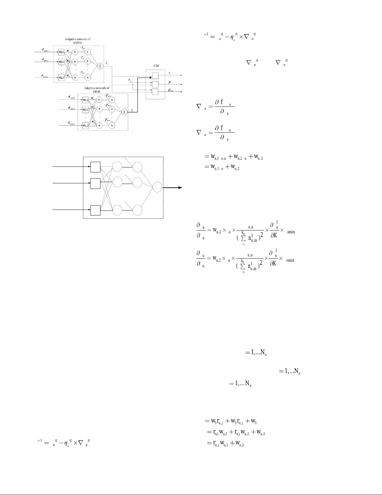
 Abstract — This study suggests a new prediction model for chaotic time series inspired by the brain e motional learning of mammals. We describe t he structure and function of this model, which is referred to as BELPM (Brain Emotional Learning - Based Prediction Model). Structurally, the model mimics the connection between the regions of the limbic system, and functionally it u ses weighted k near est neighbors to imitate t he roles of those regions. The learning algorithm of B ELPM is defined using steepest descent (SD) and the least squ are estimator (LSE). Two benchmark chaotic time series, Lorenz a nd He non, have been used to evaluate the performance of BE LPM. The obtained results have been compared w ith those of oth er prediction methods. The results show that BELPM has the capability to achieve a reasonable a ccuracy for long -term prediction of chaotic ti me series , using a limited a mount of training data an d a reasonably low computational time. Index Term s — Brain emotional learning, Chaotic ti me series , Long-term prediction , W eighted k-nearest-neighbors. I. I NTRODUCTI ON rediction models have applica tions in many di fferent areas of science and technology: b usine ss, econo mics, healthcare, and welfare services. Well-kno wn data-driven methodologies such a s neural networks a nd neuro -fuzz y models have shown reaso nable accurac y i n t he nonlinear prediction of chaotic ti me series [1]. According to the Vapnik- Chervonenkis (VC) theory [2] , a suff icient size of training samples for achieving arbitrary prediction accuracy is proportional to the nu mber of the models ’ learni ng parameters. Thus, a data-driven model with high mod el complexity and high number of learning para met ers requires a large number o f training samples to achieve high ac curac y in a prediction application. T he predictio n accurac y of predicting chaotic ti me series depends on th e characteristics of the applied models (i.e., the m odel complexity and the number of learning parameters) as well as the features of the p rediction applications (i.e., the number of training samples, cha os degree, embedding d imension , and the hor izon of prediction) [1] – [5] . This study suggests a pred iction model that co uld be feasible for long-term pred iction of chaotic s ystems (chaotic time series) with a limited a mount of training data samples ; i.e., a p rediction model with a small number o f learning parameters. Th e suggested m odel is inspired b y the brain emotional p rocessing and is therefore named BE LPM that stands for B rain E motional Learning-Based Pred iction Model . It s simple architecture has b een inspired by the brain emotional s ystem, e mphasizing the interaction betwee n th ose parts that have significant roles in emotional learning. The model mimics t he e motional learning by merging weighted k- Nearest Neig hbor (W k- NN) method and ad aptive neur al networks. T he lear ning algor ithm of B ELPM is based on the steepest desce nt (SD) and the least sq uare esti mator ( LSE). The model aims at continuing the rece nt studies that have suggested co mputational models of emotio nal p rocessing for control and pred iction applications [6 ]- [1 6]. The rest of the paper is organized as f ollows : Section II gives an introduction of emotional processing in the brain, reviews the a natomical asp ects of e motional lear ning , and gives an over view of related work in the area of computatio nal models of brain e motional learning . Section II I describes the BELPM’s architecture and illustrates its learnin g algorith m. In Sectio n IV, two bench mark chaotic time series, Lorenz and Henon, are used to evaluate the perfor mance of B ELPM a nd the results are compared with the ob tained results from o ther nonlinear lear ning methods (e.g. Adaptive-Net work-Based Fuzzy In ference S ystem ( ANFIS ) [3], MultiLa yer Per ceptron (MLP) Network [1], [2] , Radial Bias Function (RB F) Networks [1], [2] , and Loc al Linear Neuro -Fuzzy (LLNF) Models [1]). Finally, conclusions about the BELPM m odel and further improvement s to the model are stated in Sec tion V. II. BA CKG ROUN D One of the most c hallenging top ics in machine lear ning research area is develop men t of high generalization algorithms for accurate predictio n of chaotic syste ms. Recent ly, bi o - inspired models, in particular , emotion-based lear ning models [6], [8], [10], [12] -[14], have shown ac ceptable ge neralization capability in modeli ng and predicting t he chaotic behavior of dynamic systems. In fact, this capab ility i s obtained in emotion-based lear ning mod els by integrating machine learning al gorithms with th e computational m odel of emotional learning. In the following, we e xplain how emotional learning can be modeled as a co mputer-based tool and how it can b e i ntegrated with learning algorithms. T he difference bet ween BELPM and several well-known data - driven methods will also be ind icated. A. Related Works in Modeling Emotional Lea rning Since 1 988, emotion and emotional processing have been Brain Emotional Learning-Based Prediction Model For Long-Term Chaotic Prediction Applications M. Parsapoor P active resear ch topics for neuroscientists and ps ychologists . A lot of efforts have been made to analyze e motional beha vior an d describe emotion on t he basis of di fferent hypotheses, e.g., psychological, neurobiological, philosophy , and lear ning hypothesis. These hypotheses that have co ntributed to the present computer-based models o f e motional pr ocessing [18], have imitated cert ain aspects of emotional lear ning, a nd ca n be classified on the basis o f their fundamental theories and applications. For exa mple, a computer-based model that is based on t he central theory [18 ] (i.e., w hich explains ho w a primary evaluation of e motional s timuli for ms emotional experiences) is called a co mputational model of e motional learning and imitates the associative learning aspect of emotional proce ssing [18 ] that is based on fear conditioni ng [19], [ 20]. Emotional pro cessing has also been describ ed using different anato mical structures: “ MacLean’s l imbic system , Cannon’s structure , and Papez circuit ” [21 ]. The first anatomical representatio n is based on studies on cog nitive neuroscience [2 1], [ 22 ] , and has been developed on the ba sis of Cannon’s str ucture and Pa pez circuit empha sizing t he role of t he limbic system (i.e., a group of the brain regions) fo r emotional p rocessing. T he Cannon’s structure sugges t ed that the hypothala mus of the b rain pla ys t he most significa nt role in emotional learning, whi le P apez cir cuit [ 21 ] emphasized the role of the cingulate cortex in emotional proce ssing. In this study, we have f ocused o n the li mbic system, which is the basis of our suggested model. 1) Anatomical S tructure of Emotional Lea rning The limbic system i s a gr oup of b rain regions, w hich includes the hippocampus , a mygdala, thalamus, and se nsory cortex [22 ]-[24]. T he ro les of the main r egions of the limbic system with re gard to e motional lear ning can b e summarized as follows: a) Thala mus receives e motional stimuli a nd is responsible for the p rovision o f high-level information, i.e., deter mining the eff ective values of sti muli [22] -[ 28 ]. It then p asses the generated signals to t he amygdala and sensory cortex [2 8]. The thalamus includes different parts that process the emotional stimuli separatel y [2 7]. b) Sensory co rtex is a p art of the sensor y ar ea of the brain and is responsible for anal ysis and pro cessing of the received signals. T he sensory co rtex distrib utes its outp ut signal s between the amygdala a nd orbitofrontal region [ 18 ]-[ 21 ], [ 27 ]. c) Amygdala is the ce ntral part of the limbic system of mammals and has a princip al ro le in e motional lear ning [1 8]- [ 26 ]. The amygdala consists of several parts with different functional roles (see Fi g. 1 ), and it connects through them to other regions of the brain (e.g., the insular cortex, orbi tal cortex, and fronta l lobe ). It has connectio ns to the thalamus, orbitofrontal co rtex, and h ypothalamus [ 25 ] , [ 26 ]. During emotional lear ning, the a mygdala p articipates in reacting to emotional stimuli , storing e motional responses [29 ], evaluating positive a nd negative rein forcement [ 30 ], lear ning the association between unconditioned and conditioned s timuli [1 9 ], [ 20 ], [ 31 ], predicting t he association between sti muli and future rein forcement [ 31 ], and forming an a ssociation between neutral stimuli and e motionally charged stimuli [ 30 ]. Thalamous Lateral of Amygdala Basal of Amygdala Centromedial of Amygdala Emotional Response Emotional Stimulus Orbitofrontal AMYGDALA Basolateral of Amygdala Accesory Basal of Amygdala Fig.1.The parts of amy gdala and the ir pathways. T he diagram shows the pattern of fear con ditioning, which needs to be clarified [17]. The t w o main parts o f the a mygdala are the basolater al part (the largest portion o f the amygdala) a nd the cen tero medial part. T he b asolateral part has the bid irectional link to the insular cortex and orbital cortex [1 8 ], [ 20 ], [ 21 ], [ 25 ] , [ 26 ] and performs the main role in mediating m emory consolid ation [ 32 ] and p roviding the pri mary response , and is divided into three par ts: the lateral, basal , and accessor y basal [ 25 ], [ 29 ]. The lateral is the part thro ugh which stimuli enter the amygdala. Th e lateral region not only pass es the sti muli to other regions, but also memor izes them to for m t he stimul us – response association [ 31 ]. T his part also takes so me roles in spreading the sensor’s information to ot her parts, for ming the association b etween the conditioned and uncondit ioned stimuli, inhabiting and reflecting the external stimuli , and memorizing t he emotional exper iences. The basal and accessory basal parts p articipate in mediating the contextual conditioning [ 20 ], [ 25 ]. The centero medial part, which is the main outp ut for the basaloteral part [ 26 ], is divided in to the cen tral and medial parts [18 ], [ 20 ], [ 25 ] , [ 26 ]. I t is responsible for t he hor monal aspects of e motional reactio ns [ 25 ] or for mediating the expression of the emotional re sponses [ 25 ], [26 ]. d) Orbito frontal co rtex is loca ted close to t he a mygdala and has a bidirectional connectio n to the a mygdala. T hi s p art pla ys roles in p rocessing stimulus [25], d ecoding the primar y reinforcement, representin g the negative reinforcement , and learning the sti mulus – reinfo rcement associat ion. It also evaluates and co rrects reward and punishment [1 8]-[21], [33]- [37], selects goals, makes decisions for a quick response to punishment [18] , [23], [2 5]-[36], and prevents inappr opriate responses of the amygdala. The orb itofrontal cortex encompasses t wo parts, the medial and lateral. T he medial p art forms and memorizes rei nforc ement – stimulus a ssociation, a nd also has role in pro viding responses and monitoring them , whereas the lateral part evaluates the response and provides punishment [37]. 2) Emotion-In spired Computational Models Computational models of e motional learning, which are computer-based models , have b een d eveloped to represent the associative learn ing asp ect o f e motional pro cessing. From the application perspective, they can be categorize d into three groups: emotion -based decision- making model, emotion -based controller, and emotion-based machine -learning appr oach es . a) Emotion-ba sed decision- making mo del : T his model is th e basis o f arti ficial i ntelligent (AI) emotional a gent t hat integrates e motional r eactions with rational reactions. EMAI (Emotionally M otivated Artificial Intelligence) was one of the first atte mpts to develop emotion -based agents. It was applied for simulating artificial soccer playing [3 8], and its results were fairly good. T he Cathexis model [ 39 ] was another emotional agent developed that reacted to an environment by imitating an emotional decision-ma king proce ss in humans . The model of the mind [ 40 ] was developed as a modular artificial age nt to generate e motional behavior for making decisions. An agent ar chitecture that was called E motion- based Robotic Agent De velopment ( in reverse ord er, DARE) was developed o n the b asis of the somatic marker theor y; it was tested i n a multi-agent s ystem and sho wed ab ility in modeling social and e motional behavior [ 41 ]. b) Emotion-b ased c ontroller : T he first pr actical implementation of an emotion-based controller is B ELBIC (Brain E motional Learning-Based Intelligent Co ntroller) [7 ]. It was d eveloped on the basis o f Mo ren and B alken ius computational model [7], [23], [42]. T he BELBIC has been successfully emplo yed for a number of applicatio ns: controlling heating a nd air conditioni ng [ 43 ] of aerospace launch vehicle s [ 44 ], intelligent washing machines [4 5], and trajectory tracking o f stepper m otor [ 46]. Another e motion - based in telligent controller is a neuro-fuzzy co ntroller [ 47 ], which was integrated w ith e motion-based performance measurement to tune the parameters of the controller . Application o f an e motion-based controller robo tics was proposed in [48 ], which is a n interesting e xample of appl ying emotional concepts in robotic applicatio ns and imitated the reinforcement learning aspect of emotional processing . The results o f app lying emotion-based co ntrollers have shown t hat they have the capabilit y to overcome uncertainty a nd complexity i ssues o f co ntrol applications . Sp ecifically, the BELBIC has bee n proven to outperform other s i n ter ms of simplicity, reliability, and stability [7], [ 39 ]-[ 42 ]. c) Emotion -based machine-lea rning app roach : Developing machine-learning app roach es b y imitating emotio nal processing of t he brai n has captured the attention of researchers in the AI area. So f ar, some s tudies have b een carried out to develop new neural networks by i mitating so me aspects of e motional learning. Hip pocampus -neocor tex and amygdala hippoca mpus model ha ve been pro posed a s neural network models [49], [50] . The y co mbine associati ve ne ural network with e motional learning concepts. Several emotion- based prediction models [6] , [ 8] -[15] have been developed to model the co mplex systems. Most o f them ar e based on t he amygdala-orb itofrontal s ubsyste m [2 3] that was p roposed by Moren and Balkenius. They have bee n applied for different applications, e.g., auroral electrojec (AE) index prediction [ 9], solar activity pr ediction [6], [8] , [ 10], [11] -[13], [1 4] , and financial and chaotic ti me series pred iction [6] , [8]-[ 14 ]. d) Amygdala -orbitofron tal system The fundamental model of emotion-based machine-lear ning approaches and emotion -based co ntrollers is the amygdala - orbitofrontal system. It is a t ype o f computational model of emotional learnin g with a simple structure t hat has been de fined using t he theor y of t he limbic system [ 23 ]. Its structure is i nherited from some parts o f the lim bic syste m (e.g., th e a mygdala, thala mus, sensor y cortex), a nd imitates the interaction bet ween t hose parts o f the limbic systems and formulates t he emotional response using mathematical equations [ 23 ]. T he amygdala-orb itofrontal subs ystem co nsists of two subs ystems: t he amygd ala and orbitofrontal subsystem . Each s ubsystem has several linear neurons and receive s a feedback (a reward) . T he mod el’s output function has b een defined as subtracting t he orbitofrontal’s response from t he amygdala’s respo nse. To update the weights , learning r ules are de fined for both t he amygda la and orbitofrontal subsyste m . Due to its simplicity, it has been the b asis of most controllers and prediction models inspired by emotional learnin g. B. A B rief Overview of the Data- Driven Metho ds One straightforward w ay to evaluate the data-driven learning approaches (e.g., neural network and neuro-fuzz y models) is to apply them to predict chaotic time seri es . Different types of neural ne twork and neuro fuzz y models (e.g., RBF, ANFIS, LLNF) have been applied to m odel and predict the short-term a nd lon g-ter m behavior of chaotic time series (e.g., L orenz, Henon, Mackey-G lass, Ikeda) [1]-[15], [51]-[55]. We have suggested a model that differs from the previously proposed m odels i n ter ms of p rediction accuracy, structural simplicity, a nd generaliza tion capability. In the follo wing, we explain the differences between BELPM a nd other well- known data-driven models. 1) Rad ial Bias Function (RBF) d iffers fro m BE LPM i n terms of t he u nderlying str ucture, inp uts of t he ne urons, connection bet ween neurons, and number of learn ing parameters and learni ng algorithms. 2) Generalization R egression Neura l Network (GRNN) [1 ] differs from BELPM in its number of neurons ( i.e., t he number of neurons o f GRNN are equal to t he size of tr aining samples). Mo reover, GRNN has no learning algorit hm to optimize its perfor mance a nd increase its generalizatio n capability. 3) Ada ptive Neu ro Fuzzy Inference S ystem (ANFIS) and BELPM ar e not similar because of d ifferent structur es, functions, and so me asp ects o f learning al gorithms. Due to the learning algorithm and th e large n umber of lear ning parameters (linear a nd nonlinea r) that are spread through the layers, ANFIS has the cap ability to obtain very accurate results for co mplex ap plications. However, its learning algorithm has a signi ficant effect on its co mputational complexity and it also cause s over-fitting pr oblems. T he curse of di mensionality is anot her issue o f ANFIS a nd increase s the computational time of ANFIS for high-dimension app lication . Although the n umber of learning p arameters o f BELPM is not dependent on t he d imension o f input data , as mentioned before, BELPM uses Wk-NN; conseq uently, the computational ti me of BE LPM o nly depends on the nu mber of neighbors . T o decrease its time complexity in high-dimensi on ca se s, we can choose the s mall number of neighbors for the BELPM. 4 ) Local Linear Neuro Fuzzy Mo dels (LLNF) and BE LPM can both be co nsidered as t ypes of “local modeling” [ 2] algorithms. T hey b oth co mbine a n opti mization-lear ning algorithm a nd LSE to train t h e learning p arameters. Ho wever, LLNF use s Local Linear Mod el Tree (LoLiMoT) algorithm, instead of Wk-NN method of BELPM. T he number of learning para meters o f Lo LiMoT has a linear r elationship with the d imension o f input sa mples a nd number o f epochs ; thus, its computational co mplexity has no e xponential gro wth for high-dimension applicatio ns. 5) Mod ular neural network is a combination o f se veral modules with different i nputs [2] without a ny connection with others. There is no algorit hm to update the learning para meters of the modules . 6) Hybrid structures that are defined in [1], d iffer from BELPM in r eceiving th e input data . T he submodules o f a hybrid structure can al so be desig ned in parallel or series. III. B RAIN E MOTIONAL L EARNING - BASED PREDI CTION MOD EL The ar chitecture of BELPM is inspired by the brain emotional learning s ystem. It mimics so me functional and structural aspects of the lim bic s ystem region s. To describe BELPM’s architecture a nd its u nderlying learning algorit hms, we use d the machine -learning ter minology, instead of neu ro- scientific terms. For example, an input – o utput pair of training data and an input – output pair of test data ar e equivalent to an unconditioned stimulus – respo nse pair and a conditioned stimulus – response pair in neuro-scien tific ter minology , respectively. T hus, we use d t wo subscripts u and c to distinguish the training data set a nd the test d ata set that ar e defined as , , 1 { , } N c c c j c j j I r i and , , 1 { , } N u u u j u j j I r i , respectively, with c N and u N data samples. Before explaining the architecture of B ELPM, let us br iefly review t he W- kNN algorithm that is t he basic o f BELPM. T he following steps explain how the outp ut value o f a n i nput vector test i is calculated by usi ng the W-kNN algor ithm [56]: 1) Calculate the Euclidean dis tance as, j t e s t u , j 2 d ii f or each u , j i that is a member of t he training data set u , , ..., u , 1 u , 2 u ,N {} i i i . 2) Determine the k minimum values of 1 2 N u d d d , { , ... , } d as min d . T he d ata sa mples corresp onding to min d are shown as k mi n m i n , j min, j j 1 { , r } Ii , where min I denotes the samples of the trai ning data set that ar e nearest neighbo rs to the test sample, test i . 3) Calculate the outp ut of test i as given in (1). k k tes t j m i n , j j j 1 j 1 r w r w ( / ) (1) The w eight, j w , is calculated as j j w K ( d ) , where K (.) is known as t he kernel fu nction that m akes the tran sition from Euclidean distances to the weights. Any arbitrar y function t hat holds the follo wing properties given can be considered as the kernel function [56 ],[57 ]: 1) For all d , K ( d ) 0 . 2) If d 0 , then K ( d ) gets the maximum value. 3) If d , then K ( d ) gets the minimum v alue. Some typical kernel functions are the Gau ssian kernel (2), Inversion kernel (3), and t he weighted kernel f unction that is defined as (4). 2 1 d K ( d ) e x p( ) 2 2 (2) 1 K ( d ) d (3) j ma x ( ) ( d m i n ( ) ) K ( d ) ma x ( ) dd d (4) As mentioned earlier, they transform the Euclide an distances into t he weig hts; t hus, the neighbors t hat ar e closer to the test sample test i have higher w eights on esti mating the output, test r [56],[57 ]. A. Architecture o f BELPM As sho wn in Fi g. 2 , t he BELPM’s archi tecture consists of four main p arts that ar e named as TH, CX, AMYG, and ORBI , and are r eferred to as T Halamus, sensor y CorteX , AMYGdala , a nd ORBItofrontal, respec tively. MAX_MIN AGG , _ uj MAX MIN th Ouput (Unconditioned response ) j u , i j a , p j u , s CX LO MO BL CM j o , p j , o r e j a , p ORBI AMYG TH (a)During first learning Phase j r j a , p j , a r , uj AGG th Input (Unconditioned Stimulus) MAX_MIN AGG , _ cj MAX MIN th Ouput (Conditioned response ) c, j i j a , p c, j s CX LO MO BL CM j o , p j , o r e j a , p ORBI AMYG TH (a)During second learning Phase j a , p j , a r , cj AGG th Input (Conditioned Stimulus) Fig.2. The architecture of BEL PM showing the structure of each part and it s connection t o other p arts. (a) An input from training set, u nconditio ned stimulus, enters the BEL PM. (b) An input of test d ata, conditioned stimulus, enters the BEL PM. Let us assu me an unseen input c , j c I i enters BE LPM tha t provides the corr esponding output u sing the following steps: 1) T he input vec tor c , j i is fed to T H, which is the entrance part of the BELPM structure. T his part consists of two components: MAX_ MIN ( MAXimum_MINimum) and AGG (AGGregation) . T he MAX_ MIN can b e describ ed as a modular neural networ k. It has two neural networks, each of which has two layers with a co mpetitive function for the neuron o f the first la yer a nd a linear func tion for the neuro n of the second layer. The output o f MAX_MIN that is referred to as _ MA X MIN c, j th is calcu lated accord ing to (5) and is fed to AGG and AMYG. Equatio n (5) calculate s the highest and lo west values of the inp ut vector with R dimensions . T he AGG can be described as a ne ural network with R 2 linear neurons ( R is the di mension o f c , j i ); the output o f AGG, AGG c, j th , is equal to c , j i and is fed to CX a s shown in (6). M AX _ MI N c , j c , j [ M a x ( ), M in ( )] c, j th i i (5) , [] AG G cj i c, j th (6) 2) T he AGG c, j th is sent to CX, which is a pre-trained neural network with o ne layer of linear functi on. The role o f CX is to provid e c , j s and distribute it b etween A MYG and ORBI . I t should be noted that c , j i and c , j s have the sa me entity; ho wever, they have been originated from different par ts. 3) Bo th c , j s and _ MA X MIN c, j th are sent to AM YG that is th e main p art of the BELPM str ucture and i s divided in to t wo components: BL(Baso Lateral) and CM (CenteroMedial). The subpart that is re ferred to as B L cor responds to the set of the lateral and basal, while the ot her subpart, CM, correspo nds to the ac cessory b asal and c entromedial part. There is a bidirectional co nnection b etween AMYG and O RBI; this connection is utilized to exchange the infor mation, and contains AMYG’s e xpected p unishment and ORBI’s resp onse. The functionalities of AMYG have been defined to mimic some roles of the amygdal a ( e.g., storing unconditioned stimulus – response p airs, mak ing the associatio n between t he conditioned and unconditioned stimuli, and generating re ward and punishme nt). Thus, AMYG has a main r ole in providing the pr imary a nd final r esponse s. The structure and function of BL and CM are given as follows: a) BL , which is responsib le for the pro vision of the primary response of the AMYG, cal culates a , i u , j c , j u , j c , j d - 22 s s + th - th . Here, u , j s and _ MA X MIN u, j th are the output of TH and CX for each member of the tr aining data set u u , 1 u ,2 u ,N { , ,.., } i i i , respectivel y. It must be noted that c , j s and u , j s are the o utput of the CX for c , j i and u , j i , respectively. T he BL enco mpasses an adaptive network with four layers (see Fig. 3 (a)). T he first layer consists of a k nodes ( “ adaptive or square ” [3] nodes) with K (.) function (kernel function) . Each nod e has an input that is an e ntity fro m the a a min a m i n , 1 a m i n , 2 a m i n , k d , d , . . . , d d (which is a set of a k minimum distances of u a , 1 a , 2 a , N d , d , . . . , d a d ). The output vector of the f irst layer is 1 a n ; the output value of each no de of this layer is calc ulated using (7 ), where the inp ut to m th node is m d , a m in . 1 a ,m a m i n, m n K ( d ) (7) In general, the kernel functio n for m th node can be defined as (8 ), ( 9), and ( 10 ). T he input and the para meter of K (.) are determined using m d and m b , which are the m th entity of d and b , respec tively. We used the s ubscript a to d istinguish B L’s kernel function and its r elated p arameters ( a min d and a b ). m m m K (d ) e x p ( d b ) (8) m 2z mm 1 K( d ) ( 1 ( d b ) ) (9) m m ma x( ) ( d m i n ( ) ) K( d ) ma x( ) dd d ( 10 ) The seco nd la yer is a normalized layer a nd has a k nodes (fixed or cir cle), which are labeled as to calculate the nor malized value of 1 a n as (11). a 1 a , m 2 a ,m k 1 a , m (n ) n n m1 (11) The third layer h as a k cir cle nodes w it h functions g iven in ( 12 ). This layer has t wo input vectors, 1 a n and u a r ; the latter i s a vector that is extracted from u u u , 1 u , 2 u , N r , r , . . . , r r and is related to the a k nearest neighbors . a 1 a , m 3 a ,m u a , m k 1 a , m (n ) n r n m1 (12) The fourth layer ha s a single node (circle) that calculates the summation o f its input vecto r to produce a , j r , the p rimary output (response). The f unction o f the third and fourth layer s can be formulated acc ording to (1 3), i.e., the inner p roduct of the third la yer ’ s output, 3 a n , and a r u . 3 a , j a u a r nr (1 3) The provided p rimary r esponse, a , j r , is sen t to the CM to calculate t he reinforcement signal. It shou ld b e noted that the connection bet ween CM and B L (see Fig. 2( a)) does not exist between centro medial nuclei and the other parts o f the amygdala. Ho wever, we assu me d it s existe nce in the BELPM’s architecture. b) CM is resp onsible to provide the final output; th us, it is an important co mponent o f A MYG . It has inputs from B L a nd ORBI, and perfor ms different functions during the fi rst leaning phase and t he second lea rning phase of the BE LPM.  CM during the first lea rning phase : T he first learnin g phase of BELPM begins when the input of BE LPM is chosen from the training sets, u u , j u , 1 u , 2 u ,N u , ,..., i I i i i (see Fig. 2(a)). After receiving this inpu t, BL starts performing it s function and provides r a, j and , uj r that are sent to CM, which has t hree square nodes (see Fig. 3(b)). The function of the first nod e is d efined acco rding to (14) to provide j r , i.e., the outp ut of BELPM (emotional response). The functions of the second and third nodes ar e d efined accor ding to (15) and (16), which provide reinforcement ( punishment), j a p , , and expected reinforce ment (expected punishment) , e a , j p , respectively. j 1 a , j 2 o , j 3 r w r w r w (1 4 ) a , j a , 1 u , j a , 2 a , j a , 3 p w r w r w (1 5) e a , j u , j a , j p r r (1 6 ) A supervised learning algorith m determines app ropriate valu es for the weights.  CM during the seco nd lea rning phase : T he seco nd learning phase of BELPM begins when t he i nput is chosen fro m t he test data se ts c , j i (see Fig. 2(b )). As BL has no i nformation about the desired output ( t he target respo nse), it does not send an y informa tion about the d esired outp ut to the CM. In t his phase, the first node of the CM has the sa me input and per forms the same function as it does in the fir st learni ng phase. However, the input and the connection of t he second square node are different. In thi s phase, the reinforcement, j a p , , is calculated according to (17), which differs f r om (15) in terms of its in put. The third node has no input and function , and it can b e removed. a , j a , 1 j a , 2 a , j a , 3 p w r w r w (1 7) 4) T he expected reinforce ments, e a p , and c , j s are sent to ORBI that is co nnected to CX and AMYG. T he function of this part is d efined to e mulate certain ro les o f the orbitofron tal cortex. These roles include forming a s timulus – reinforce ment association, evaluati ng reinforcement , and providi ng an output. Before explaini ng how ORBI performs, it should be noted that ORB I starts performing its functions after receiving the vector of the expec ted reinforce ment, e a p , which means that BL of AMYG must have fulfilled its functions. T he ORBI is composed o f MO and L O correspo nding to th e lateral a nd medial parts of the orbitofrontal cortex, and their functions are described as follo ws: a) MO , which is respon sible f or th e pro vision of the secondar y response of the BE LPM, receives c , j s and calculates o , j c , j u , j 2 d ss for each u , j s . T he MO consists of a four- layer adaptive net work. T he first la yer has o k nodes (square ), and the input vector and output vector of the first la yer’s nodes are o min d (t he o k minimum va lues o f the distance vector, u o o , 1 o , 2 o , N d , d , . . . , d d ) and 1 o n , respectively. Th e function of m th node is the kernel functio n give n in (1 8 ). o m i n , m 1 o ,m n K ( d ) (1 8) The seco nd layer co nsists of o k nodes. Each node calculates an output as shown in (1 9) and sends it to the third layer. o 1 o , m 2 o ,m k 1 o , m (n ) n n m1 (19) The third layer has an i nput v ector e a min p , which is a vector o f o k minimum values of e a p corresponding to o min d . The th ir d layer’s nodes have the functi on to multiply e a min p and 2 o n , as given in (20). e a m i n 3 2 o o n n p (20) The fourth layer has a single node with a summation functio n that provides the o utput o f ORBI (the secondar y response) . The result o f t he third and fourth la yers can be obtained according to ( 21) . The output , oj r is fed to the LO and CM. 2e o , j o a m i n r np ( 21 ) b) LO evaluates the output of MO , generates o , j p as reinforcement (punishme nt), and sends it to MO . It has o ne node (square) with a summation function given in (2 2 ). o, j o , 1 o , j o , 2 p w r w (2 2) The main structure of BELPM is similar to the a mygdala - orbitofrontal model. However, the connectio n between the components, their functions, and d efinition of reinforce ment functions are signi ficantly different fro m t he a mygdala - orbitofrontal model . Moreover , in this study, we have used pre-trained neural net works to explai n the functionality o f TH and CX; however, to increase the functionality and adaptability o f BELPM, they can be defined b y a multi -la yer NN with trainable weights. K(.) K(.) N N N K(.) × × × ∑ . . . . . . . . . 1 min, a d k a min, d 2 min, a d 1 a,1 n 1 a,2 n 1 k a, n ua,1 r ua,2 r k ua, r a r Adaptive network of AMYG (a) (b) × K(.) K(.) N N N K(.) × × × ∑ . . . . . . . . . 1 min, o d k o min, d 2 min, o d 1 o,1 n 1 o,2 n 1 k o, n e amin,1 p o r e amin,2 p e k amin, p Adaptive network of ORBI (c) Fig. 3. (a). The adaptive network of BL. (b). The adaptive networks of AMYG and ORB and C M. (c). The ada ptive netw ork of ORBI. B. Learning Algorithms of B ELPM In the following, we e xplain how the BE LPM uses the combination of t wo lear ning methods: the SD [3] and L SE to learn t he i nput – output m a pping (t he stimulus – response association). T he learning p arameters are the weights ( 1 2 3 w , w , w , etc . ) and the para meters of kernel functio ns ( o b and a b ). As mentioned earlier , the lear ning algorith m of BELPM is divided into two phases: the first lear ning pha se and the second learning phase. Each of them uses different learning rules to ad just the learning par ameters. 1) First lear ning p hase : At the first learning p hase, a hybrid learning algorithm [3] that i s a co mbination of SD a nd LSE is used to update the learning parameters of AMYG (e.g., a b , , a , 1 a ,2 ww and 1 2 3 w , w , w ) and O RBI ( o o ,1 o ,2 , w , w b ). Under the assumption that the linear parameters, 1 2 3 o ,1 o ,2 a , 1 a ,2 a ,3 w , w , w , w , w , w , w , w have fixed val ues, the nonlinear para meters ( kernel par ameters), o b and a b , are updated by SD in a batc h-learning ma nner. T hus, SD is applied to minimize the t wo loss function s, which have b een defined on t he b asis o f a p and o p . Equations (2 3) and (24 ) are SD-based learnin g rule s used to calculate the derivatives of the loss functions, with respec t to o b and a b . a it 1 i t i t i t a a a η b b b (2 3) o it 1 i t i t i t o o o η b b b (2 4) The parameter it denotes the current values o f learn ing parameters, where it a b and it o b are the gradients of lo ss functions to t he para meters o b and a b (2 5) and (2 6). T wo learning rates a it η and o it η are defined as functions of a p and a p . a a a f (p ) b b (2 5) a a a f (p ) b b (2 6) where a p and o p are defined using ( 27) and ( 28 ). a , 1 u , a a , 2 a a , 3 w w w a p r r (2 7) o o , 1 o o , 2 ww pr (2 8) The ORBI and AMYG have their own loss function and update th eir o wn lear ning par ameters o b and a b separately. T he derivatives of (2 5) and (2 6) are for mulated by using the ch ain rules o f (2 9) and ( 30 ). Here, we ha ve ignored it and j ust mentioned about t he chain ru les, but in the al gorithm, it has been calculated for the current iteration , it . a m i n a 1 u , a aa a , 2 a k 1 a a , m w 2 K ( n ) m1 r pn rd b (2 9) o m i n o 1 u , o oo o , 2 o k 1 o o , m w 2 K ( n ) m1 r pn rd b ( 30 ) An offline version of LSE is used to update t he linear parameters under the as sumption that the nonlinear parameters have been updated and their value s are fixed. T he output o f BELPM, j r , is p arameterized b y the weights, { ,, 1 2 3 w w w } . Furthermore, a , j p and o , j p have been for mulated usin g the linear para meters, ,, a , 1 a ,2 a ,3 w w w , o , 1 w , and o ,2 w , acco rding to (2 7) and (28) . T he LSE updates the weights 1 2 3 w , w , w , ,, a , 1 a ,2 a ,3 w w w o , 1 w , and o ,2 w by ass uming that each tr iple o f the set a , j o , j u , j u {( r , r , r ), j 1 , . . . N } is substituted into ( 14 ). Each triple of a , j u , j a, j u {( r ,r , p ), j 1 , . . . N } a nd each pair of o , j o , j u ( r , p ) ,i 1 , . . . N are also substituted into (1 5) and (2 2), respectively; thus, u N linear equations s uch as (31), (3 2), and (33) are derived. u, j 1 a , j 2 o , j 3 r w r w r w ( 31 ) a, j u , i a , 1 a , i a , 2 a , 3 p r w r w w (3 2) o, j o , j o , 1 o , 2 p r w w (3 3) Equations ( 31 ), (3 2), and (33) can be rewritten in matrix for m as N u a , j o , j j 1 r r 1 A , u N u , j a , j j 1 r r 1 B and u N o , j j1 r1 C to define (3 4), (35), and (36 ), and update the li near para meters using LSE. Here, th e weights are defined as ] [ 3 2 1 ,w ,w w  w , ] [ a ,3 a ,2 a ,1 ,w ,w w  a w , and ] [ o ,2 o , 1 ,w w  o w . T 1 T u w (A A) A r (3 4) T 1 T e aa w ( B B) B p (3 5) T 1 T e o o w (C C) C p (3 6) During t he first learn ing p hase, the lear ning parameters, linear and nonlinear , can b e updated by usin g o ne of t he follo wing methods:  All parameters can b e updated using SD .  T he nonlinear para meters can b e updated using SD and the i nitial values of linear p arameters ca n be adjusted using LSE.  T he linear p arameters ar e updated using LSE and the initial valu es of para meters of kernel functions are chosen by using a he uristic method.  T he nonlinear para meters are updated using SD and LSE are applied to update the linear para meters. Certainly, these methods differ in terms o f time co mplexity and pred iction accuracy, and a tradeoff between hig h accurac y and lo w co mputational time must be considered to choose a feasible method. T he batch mode or online mode of each method can be co nsidered for the first learning p hase. 2) Second learning phase : At the second learni ng p hase, the nonlinear and kernel para meters are updated by a reinforcement-lear ning algorithm. T he nonlinear par ameters are updated by SD . The SD algorithm minimizes the lo ss functions, which are defined based o n the reinforcements, a , j p and o , j p , usin g (3 7) and (28). It must be noted that a p is calculated using the obtai ned outpu t of BELPM, r , as gi ven in (37 ), which d iffers fro m that calculat ed u sing (27) . T he adjusting rules that update o b and a b are calculated accordin g to (21) and (22). The d e rivatives of the los s functions with resp ect to o b and a b are calculated according to (30) and (3 8). Here, the weights a , 4 a ,5 a ,6 w , w , w are equal to [1, -1,0]. a , 4 a , 5 a , 6 w w w aa p r r (3 7) 1 u, aa 45 k 2 n ww K ( n ) a a, a, a amin aa a,m m1 r p r rd bb (38) IV. CASE ST UDIES: CH AOTIC T I ME SERIES In this sectio n, BELPM is evaluated as a pred iction model by using t wo benchmar k chaotic time series, Lorenz and Henon. To provide a careful comparison with other methods, we used vario us d ata sets with different initialized points and sizes o f training samples. We also utilize d t wo erro r measures: normalized mean sq uare error (NMSE) and mean square error (MSE), as given in ( 39 ), (4 0), to assess the perfor mance of t he prediction models and provide results comparable w ith ot her studies. N 2 jj j1 N 2 jj j1 ˆ (y y ) NMSE (y y ) ( 39 ) N 2 jj j 1 1 ˆ MS E ( y y ) N (40) Where ˆ y and y refer to the observed values and desired targets, respec tively. T he p arameter y is the average of t he desired targets. For all e xperiments, one -fold cr o ss -validatio n was c hosen; the nu mber o f samples in one -fold cros s- validation was equal to the size o f the test data set. A. Lorenz Time Series The Lorenz ti me series [5], [9], [ 58 ] was chosen as t he f irst test, given by using ( 41) and (42). In this case study, the initialized point is acco rding to x (0 ) 1 5 , y ( 0 ) 0 , z ( 0 ) 0 . . x a( y x ) . y bx y x z . z x y c z (4 1) a 1 0 ,b 2 8 , c 8 / 3, T 0 . 0 1 s (42) To produce the time series, the sa mpling period is equal to 0.01 s [5], [9], [ 58 ], and the e mbedded dimension is selected as three. T he BELPM is teste d for fo ur sets o f data from t he Lorenz time serie s. T he first data set is selected from 32 nd to 51 st s, and is employed for long-ter m prediction. For the training set, 5 00 samples are used and the next 14 00 samples are considered as the test data set and validation data set . Table I presents the NMSE s obtained fro m applying d ifferent methods for 10 , 30, and 40 steps ahead pred iction of this data set. It also indicates that the NMSE of ANFIS is lo wer than the NMSE o f BE LPM for 10 s teps ahead pred iction. Ho wever, when the pred iction horizon increases to 30 and 40 steps ahead, the NMSE s o f B ELPM are lo wer t han A NFI S. The presented results in Tab le I also show that an increa se in the prediction horizon causes a d ecrease in the predictio n accuracy for all met hods. I t is important to note that the NMSEs of BE LPM for pr edicting 30 and 40 steps a head ar e less than those of the o ther methods. For the second data set, ANFIS, Wk- NN , and B ELPM are tested for 1 – 20 steps a head prediction , using 150 0 samples as the training data set and 100 0 samples as t he test data set. In Fig. 4, the NMSE values v s. the prediction steps are d epicted ; it ca n be o bserved that the NMSE values of BELPM ar e lower than those o f the other methods, especially, i n the case of 15 steps ahead predictio n and longer. TABLE I THE COMPARISONS OF NMSE S OF DIFFERENT METHOD S TO PREDICT MULTI - STEP AHEAD OF L OREN TIME SERIES (T HE FIRST DATA SET ) Learning Method Ten Thirty Forty BELPM 0.0125 0.2473 0.2447 ANFIS 0.006 0.3559 0.3593 RBF 0.4867 [ 58 ] 0.3405 0.6887 LLNF 0.1682 [ 58 ] 0.4946 0.5341 Wk- NN 0.0235 0.2599 0.3830 0 2 4 6 8 10 12 14 16 18 20 0 0.005 0.01 0.015 0.02 0.025 St eps A hea d NMSE BE LPM ANFI S W KNN Fig.4. The NMSE values of multi-step ahead prediction of Lorenz system v s. prediction horizon for 1000 samples of test data u sing 1500 sam ples as training data ( the second data set). The dotted curves show the NMSE of BELPM. In the th ird data set, ANFIS, Wk -NN, a nd BE LPM are compared for 30 steps ahead pred iction, with diffe rent size s o f training data set. I n t his case, the complete sample set is chosen from 30 th to 5 5 th s , and the training is co nducted using 500, 1000 , and 1500 samples to pred ict 1000 samples of test data set from 45 th to 55 th s. The validatio n set is 10 00 samples fro m 56 th to 65 th s. Table II co mpares the values of NMSE for the d ifferent methods and once again shows t hat NMSE of BELPM has the lo west value among that of all the methods tested. For the fourth data set, the t raining set and test data are picked from 15 th to 45 th s and 46 th to 55 th s, respectively. BELPM is applied for 25 steps ahead pr ediction and the NMSE values, CPU ti me, and structures of different models are compared in Tab le III. Again, i t can be observed that the NMSE of BE LPM is lowe r th an t hat of the other methods. The time co mplexity of BELPM is less than m ost of the other methods, and only Wk- NN is found to have a little lower time complexity than BE LPM. TABLE II THE COMPARISONS OF NMSE S OF DIFFERENT METHOD S FOR THIRTY STEPS AHEAD PREDICTION OF LORENZ TIME SERIES U SING DIFFERENT SIZES OF TRAINING SAMPLES . Learning Method 500/1000 1000/1000 1500/1000 BELPM 0.1711 0.0108 0.0280 ANFIS 0.4199 0.1002 0.0947 Wk- NN 0.1951 0.1518 0.0425 TABLE III THE COMPARISONS OF NMSE S , CPU TIME A ND STRUCTURE OF DIFFERENT METHODS TO PREDICT 25 STEP S AHEAD USING 3 000 TRAINING DATA SAMPLE S Learning Method NMSE TI ME(Sec) STRUCTU RE BELPM 0.0325 11.81 10neuron ANFIS 0.0802 12.91 4 rule LoLiMoT 0.2059 18.74 7 neuron RBF 0.1193 26.07 32 neuron Wk- NN 0.0342 1.23 5 neighbor As mentioned earlier, the Lorenz chaotic ti me series i s a well - known b enchmark time ser ies and has bee n te sted with numerous data-driven models to eval uate the models ’ performance. T able I V presents t he obtained NMSEs of several data-dri ven methods for noiseless and noisy data. T he data-driven models are: Nonlinear Autoregres sive model with eXogenous input (H ybrid N ARX -Elman RNN) [59 ], Evolving Recurrent Ne ural Ne tworks (ERNN) [ 60 ], Radial Ba sis Function ( RBF), multilayer per cep tron ( MLP) [ 5], Support Vector Regression (SV R), Tapped Dela y Line M ultila yer Perceptron (TDL-MLP), Distrib uted Local Experts based on Vector_Quantization using Information T heoretic learning (DLE-VQIT) [ 61 ], C ooperative Coevolution of Elman Recurrent Neural Networks (CCRNN) [ 62 ], Functional Weights Wavelet Neural Network -based state-dependent Au toRegressive (FWWNN- AR ) [63], Recurrent Neural Network trained w ith R eal -time Recurrent Learning (RNN - RTRL), Recurrent Neural Ne twork trained with the second - order Extended Kalman Filter (RNN-EKF), Recurrent Neur al Network trai ned with the algorith m and Bac kProp agation Through Time (BPTT) , f eedforward Mu lti layer Perceptron trained with the Ba yesian Levenberg – Marquardt (MLP-BLM) , and recursive second-ord er training of Rec urrent Ne ural Networks via a Recursive B ayesian Levenberg – Marquardt (RBLM-RNN) algorithm [6 5] . It ca n be noted that the table is sorted according to the ob tained NMSEs , and that the NM SE of BELPM is not excellent as that o f the other methods . Howev er , this table co mpares the NMSEs for short-ter m prediction, which is not a feasible ap plication for BELPM. B. Henon Time Series The seco nd bench mark of this study is the Henon t ime series that is constructed by using (4 3 ). 2 x(t 1 ) 1 a x ( t) y ( t) y(t 1 ) b x ( t) a 1 . 4 , b 0 . 3 (4 3) The embedded dimension ar e considered as 0.01s [5 ], [ 58 ] and three , r espectively. I n t his case stud y, t he initialized point is x ( 0 ) 0 , y( 0 ) 0 . Three data sets of the Hen on time series are used for evaluating the BELPM. T he first data set is selected from 9 th to 18 th s and the training data set a nd the t est data s et co nsist of 800 and 100 samples, respecti vely. The BELPM, ANFIS, a nd W k-N N ar e tested to pred ict three steps ahead of this data set . TABLE IV THE COMPARISONS OF NMSE S OF DIFFERENT METHOD S FO R LORENZ TIME SERIES Learning Method NMSE No of Training and Test Fundamental Method and steps ahead data samples FWWN N[63] 9.8e- 15 1500,1000 NN+AR, 1 ste p noisele ss NARX[59] 1.9e- 10 1500,1000 AR, 1 step noise less BELRFS[12] 4.9e- 10 1500,1000 NF+BEL , 1 step noisele ss ERNN[60] 9.9e- 10 1500,1000 NN, 1 step noise less RBF[5] 1.4e-9 1500,1000 NN, 1 step noise less MLP[5] 5.2e-8 1500,1000 NN, 1 step noise less BELPM 2.9e-6 1500,1000 W-kNN+BEL ,1st ep noisel ess TDL-MLP [61] 1.6e-4 ----- NN, 1 step noise less DLE-VQI T[ 61 ] 2.6e-4 ----- ----- , 1 step noiseless LSSVMs[64] 6.4e-5 1000,250 NF, 1 step noisy -STD 0.05 BELPM 3.7e-4 1500,1000 W-kNN+BEL ,1 stepnoisy- STD 0.001 BELPM 4.4e-4 1500,1000 W-kNN+BEL ,1 stepnoisy- STD 0. 01 RBLM- RNN[65] 9.0e-4 1000,250 RNN,1 step noisy -STD 0.05 CCRNN [62] 7.7e-4 500,500 NN,2 step noise less LLNF [64] 2.9e-4 1000,250 RNN, 1 step no isy-STD 0.05 MLP_BLM[65] 8.1e-4 1000,250 NN, 1 step noisy -STD 0.05 MLP_EKF [ 65] 1.6e-3 1000,250 NN, 1 step noisy -STD 0.05 RNN- RTRL [65] 1.7e-3 1000,250 NN, 1 step noisy -STD 0.05 RNN-BPTT [65] 1.8e-3 1000,250 NN, 1 step noisy -STD 0.05 RNN-EKF [65] 1.2e-3 1000,250 RNN,1 step noisy -STD 0.05 BELPM 1.0e-3 1500,1000 W-kNN+BEL ,1 stepnoisy- STD 0.1 Table V presents the NMSEs, structure, and computational time (CP U ti me) for the teste d methods. It can be noted th at the NMSE of BELPM is lowe r than that of the o ther method s. This table also indicates t hat the number of neurons i n BELPM is more than t he number of rules in ANFIS; however , the CP U time for BE LPM is lesser than tha t of ANFIS. The graph in Fig. 5 displays the obtained error s (the diff er ence between the tar get val ues and o btained outputs) from ANFIS and BELPM for the t est data set. We have also co mpared t he effect of di fferent structures of W-kNN, ANFIS, a nd BELPM on their prediction ac curacy. T he structures o f these methods have been c hanged by increa sing the number of nei ghbors in BELPM and Wk-NN and the number of rules in ANFIS . As Fig. 6 shows the value o f NMSE for ANFIS decrea ses when the number of r ules increas es. In contrast, increasi ng the number of nei ghbors o f Wk -NN increase s the value of NMSE. For BELPM, the value of NMSE decrease s slo w ly when the number of neighbors increases. This experiment verifies the generalization ca pability o f BELPM and shows that different structures of BELPM d o not make a noticeable d ifference between the o btained prediction erro rs. T o further evaluate the performance o f the BELPM and verify its robustness, white noise with sta ndard deviation 0 .1 is added to the first data set, and the results of multi-step ahead p rediction are listed in Table V. The effect o f using the second learni ng phase of BELPM has bee n prese nted in T able VI. I t is clear t hat there is a r eduction in the obtained NMSEs of B ELPM because o f the second learning phase (S LP). 0 10 20 30 40 50 60 70 80 90 100 -0.3 -0.2 -0.1 0 0.1 0.2 0.3 0.4 0.5 0.6 T I ME(Sec) Thre e St eps A hea d Prediction E rro r ANFIS BELPM Fig. 5. The obtained erro r of three st eps ah ead predictions of the Henon time series by BELPM and ANF IS. TABL E V THE COMPARISONS OF NMSE S , CPU TIME AND STRUCTURE OF DIFFERENT METHODS TO PREDICT THREE STEPS AHEAD OF H ENON T IME SERIES ( FIRST DATA SET OF H ENON ) Learning Method NMSE Structure CPU Time(S ec) BELPM 0.0065 27neuron 0.3315 RBF[5] 0.0872 42 neuron ------- LoL iMoT[5] 0.0291 20 neuron ------- ANFIS 0.0232 25rule 153.3 WKNN 0.0107 5 neighbor 0.0725 4 9 16 25 0 0.05 0.1 0.15 0.2 0.25 0.3 0.35 0.4 Number of Neuro ns OR Rules NMSE Error BELPM ANFIS WKNN Fig. 6. The comparison of NMSEs of three different structures obtained using the BELP M, ANFIS, a nd W-kNN. These methods have been used for different struc tures. TABLE VI THE COMPARISONS OF NMSE S OF DIFFERENT METHOD S TO PREDICT MU LTI - STEPS AHEAD OF H ENON TIME SERIES Learning Method 1Step-ahead 2Step-ahead 3Step-ahead BELPM(SL P ) 0.0063 0.0251 0.1436 BELPM(FL P ) 0.0066 0.0274 0.1576 ANFIS 0.0051 0.0244 0.2539 LoL iMoT 0.0590[5] 0.2475 0.70 48 WKNN 0.0078 0.0479 0.1897 The graph in Fi g. 7 show s t he values of NMSE of two steps ahead p rediction of the first data set during t he lear ning phases. It can be observed that the NMSE d ecreases continuously duri ng the first and second learning pha ses. T he graph in Fig. 8 dep icts the mean square error ( MSE) that is obtained fro m the training samples a nd test samples during the first learnin g phase. I n each epoch, the lear ning parameters have bee n updated and the values of MSE for the trai ning d ata and the test data have b een ca lculated. It is noticeable that the values o f the dotted curve that is r elated to the MSE of the test data are lower than those o f the solid curve, i.e., the MSE o f training data. 0 5 10 15 20 25 30 35 40 45 0.0256 0.0258 0.026 0.0262 0.0264 0.0266 0.0268 epo chs NMSE err or indexes pre diction erro r of noisy data (First and s econd lear ning phase) Error s of s econd lear ning phase Error s of first learning phase Fig.7. The NMSE of BEL PM to predict the two steps ahead of Henon time that is added white noise with standard deviation 0.1. The solid line is related to the NMSE during 35 epochs of the first learning phase and the dashed line is the NMSE during 10 epoc hs of the se c ond learning phase. 0 20 40 60 80 100 0 0.2 0.4 0.6 0.8 1 1.2 x 10 -5 epochs Mean Squar e Error T est T rain Fig.8. Curves of the mean square error during the first learning phase; the solid line is the MSE c urve, w hich is related to training data; the dashed line is the MSE curve, w h ich is related to te st data. The seco nd data set of the Henon ti me series is selected from 8 th to 1 8 th s, and three d ifferent sizes of data samples are selected as training data. Table V I I compares the obtained results from e xamining di fferent methods that ar e trai ned by different trai ning set s: 300, 600, and 900 training sa mples, and have been used to p redict 100 samples of test data. As sho wn in Table VI I, the pred iction accurac y of BELPM is higher t han that of the o ther met hods in all cases; thus, it is a suitab le method for the pred iction ap plication with a s mall number of training sa mples. The bar char t in Fig. 9 sho ws the NMSE for the compared methods. I t ca n be seen that the values of NM SE of B ELPM are once again lo west a mong t hose of all t he presented methods. Exami nation of this d ata set re vealed that a decrease in the number o f training samp les ca uses an increase in the values o f NM SE of all met hods (e.g., BELP M, ANFIS, W k- NN , a nd RBF). Ho wever, the rate of increasing the values o f NMSE of BELPM is lower than that of other methods. The third data set of the Henon time series is selected to co mpare the tim e co mplexities (CP U ti me) of various lear ning met hods when the size of the training set is large. A training set of 3000 sa mples are selected from 100 th to 130 th s, and the following 100 0 samples from 130 th to 140 th s are considered as the te st d ata set. Tab le VIII su mm arizes the NMSEs, CPU time, a nd the applied structures of the dif ferent methods. Although the CPU time of Wk -NN is 1.128 s, which is less t han that of B ELPM, the prediction accurac y of BELPM is higher than t hat of Wk -NN and other methods. TABLE VII THE COMPARISONS OF NMSE S OF DIFFERENT METHOD S TO PREDICT 100 DATA SAMPLES USING DIFFERENT NUMB ER OF NUMBER OF TRAINING SAMPLES Method 900/100 600/100 300/100 BELPM 0.0067 0.0102 0.0269 ANFIS 0.0301 0.0406 0.0538 WKNN 0.0107 0.0118 0.0468 RBF 0.0155 0.0307 0.0457 100 300 600 900 0 0.02 0.04 0.06 0.08 0.1 0.12 0.14 Numb ero f train ing data NMSE err or indexes ANFIS BELP M W KNN Fig. 9. The NMSE of different methods for three step s ahead p rediction of Henon time series using different sizes of training data (100, 300, 600, and 900) for 100 sampl es of test da ta. TABLE VIII C OMPARISON OF DIFFERENT METHO DS TO PREDICT THREE STEP AHEA D OF HENON TIME SERIES FOR THIRD SET OF DATA Learning Method NMSE TI ME(Sec) STRUCTU RE BELPM 0.0077 5.72 5neuron ANFIS 0.0514 627.56 16 rules LLNF 0.2059 18.74 7 neuron RBF 0.1193 26.07 32 neuron WKNN 0.0083 1.128 3 neighbor Fig ure 10 displa ys t he o btained errors from exa mining BELPM and ANFIS for three step s ahead pr ediction. The figure shows that B ELPM is more accurate than ANFI S. Fig ure 11 depicts ho w the NMSE index of BE LPM d ecrease s over its lear ning phases. It b ecomes obvious that for b oth training and test data , there is a co ntinuous decr ease in t he NMSE index d uring the epoc hs. For this e xperiment, we have applied BELPM for the third data set and have chosen 200 epochs for both first and sec ond learning phases. Thi s fi gure verifies the ability of B ELPM to adjust the learni ng parameters in the online mode. 0 100 200 300 400 500 600 700 800 900 1000 -0.8 -0.6 -0.4 -0.2 0 0.2 0.4 0.6 0.8 TI ME (sec) ERROR ANFIS BELPM Fig.10. The prediction errors of ANFIS an d BELPM for t hree step s ahead prediction of Henon time ser ies using 3000 tr aining sample s. 0 50 100 150 200 1.978 1.979 1.98 1.981 1.982 1.983 1.984 x 10 -3 epo chs NMSE err or indexes Error of t ra ining da ta (First learnin g pha se) 0 50 100 150 200 7.8 7.805 7.81 7.815 7.82 7.825 7.83 7.835 7.84 7.845 x 10 -3 epo chs NMSE err or indexes Error of T est data (First lear ning phase) (b) Fig.11. The NMSE of th ree step s ahead predictions during first learning phase. (a) Fo r training data. ( b) For te st data. The Henon chaotic time series is also a well-known benchmark time series, and has bee n examined by a large number of data -driven model s. T able IX lists the obtained NMSEs of several data -driven methods. It b ecomes obvious that BELPM has a fairly good performance in predicting noisy data time series. TABLE IX THE NMSE VALUES OF D IFFERENT METHODS TO PRED ICT H ENON TIME SERIE S Learning Method NMSE No of Training and Test data samples Fundamental Method and time series RBF[5] 1.4e-9 1500,1000 NN, 1 step noise less MLP[5] 5.2e-8 1500,1000 NN, 1 step noise less TDL-MLP [ 61 ] 1.6e-4 ----- NN, 1 step noise less DLE-VQI T[61] 2.6e-4 ----- ----- , 1 step noiseless BELPM 3.3e-4 800,100 W-kNN+BEL , 1 st ep n oisy- STD 0.001 LSSVMs[64] 4.4e-4 1000,250 NF, 1 step noisy -STD 0.05 RBLM- RNN[65] 6.8e-4 1000,250 RNN,1 step noisy -STD 0.05 RNN-EKF [65] 8.6e-4 1000,250 RNN,1 step noisy -STD 0.05 LLNF 7.7e -4 1000,250 RNN, 1 step no isy-STD 0.05 MLP-BL M[65] 8.1e-4 1000,250 NN, 1 step noisy -STD 0.05 BELPM 6.4e-3 800,100 W-kNN+BEL ,1 st ep n oisy- STD 0.01 RNN-BPTT [65] 1.1e-3 1000,250 NN, 1 step noisy -STD 0.05 RNN- RTRL [65] 1.0e-3 1000,250 NN, 1 step noisy - ST D 0.05 V. DISCUSSI ON AND C ONCLUSIO N This study has presented a prediction model inspired by brain e motional processi ng and, par ticularly, has investi gated this model for chaotic time series pred iction. We have described the architecture of this mo del usin g feedfor ward neural networks a nd adap tive networks . Further more, w e have also explain ed the function and learning al gorithms of the model that is referred to as B ELPM. The accurac y of the BELPM has been extensively evaluated by different data s ets of two b enchmark chaotic time series, Lorenz and Henon, and the results strongl y indicate that the model can predict the long-term state of c haotic ti me series rapidl y and more accurate ly than other well-kno wn methods, i.e., RBF, LoLiMoT, and ANFIS. T he results also show t hat B ELPM is more e fficient than the ot her methods when lar ge traini ng d ata sets are not available. In comparison with other data -driven appro aches, we can summarize the highlighted features of BELPM as follows: 1) It converges ver y fast into its optimal structure (see Tab les III, IV, and VII). 2) I t h as high generalization capability (see dotted lines in Fig s. 7 and 8), high r obustness fro m the perspecti ve of learning al gorithms ( see solid lines in Figs. 7, 8, 11, and 12) , low noise sensitivity (see Table V) , relatively low computational time (compare the values of ti me columns in Tables III, I V, and VII), and low model complexity. 3) The number of nei ghbors in AMYG and ORBI is not dependent on the input ’s di mension, which indicate s that th e dimension of data does no t have a direc t effect on the model complexity. Ho wever, the i nput’s di mension increases the computational time o f calc ulating the Euclidean dista nce a nd searching t he nearest neighbors; thus, it has a n indirec t effect on t he co mputatio nal time of BELPM. The experi ments have also shown that when there are a limited number of samples for training the model, the number of neig hbours, o k and a k should be raised to get accurate results (co mpare Ta ble I V and VII) . A general o bservation is that a better pred iction result could be achie ved when the number o f neighbours, o k , in the ORBI part is appr oximately t wice the number of neighbours, a k , in the AMYG part. T he feasible values and effective combinatio n of a k and o k can be deter mined using meta-heuristic opti mization methods (e.g., genetic algorit hm) . 4) The second learning p hase o f BELPM provides onli ne adaptation and continuousl y increases the p rediction accura cy and offers the capability to overco me b oth over -fitting and under-fitting proble ms. 5) For long-term pr ediction u sing a small number of trai ning samples, the acc uracy of B ELPM is higher than other da ta - driven models, such as ANFIS and LoLiMoT (see Tab les I, II, IV , and V). In the case of using a large n umber of training samples, it is also noticeable that the computational time of BELPM is not greater t han t hat of ANFIS a nd LoLiMoT (see Tables III and VII). It can al so be co ncluded that when the degree o f chaos is high, e ven usi ng a large nu mber of data a nd neuro-fuzzy methods ( ANFIS and LoLiMoT ) would not achieve hi gher pred iction a ccuracy than the BELPM (see Table VII) . As future w orks, the authors consider adding some optimization methods (e.g., g enetic algorithm) to find optimal values of the fiddle par ameters, e.g., the number of neighbo rs a k and o k and the initial values o f no nlinear parameters . O ther improvements in the model would be made on the basis of kd- Tree d ata structure [47] to add ress “the curse of dimensionality” [1] problem and decrease the com putational time co mplexity o f BELPM. To ad just the nonlin ear parameters , d ifferent t ypes of opti mization methods (e. g., Quasi-Newton or Conjugate Directions) for ORBI a nd AMYG can be u tilized. In addition, the Temporal Difference (TD) learning al gorithm ca n also be used as a reinforce ment metho d for the second learning phase to update the linear learning parameters. The goo d re sults obtained b y emplo ying the BELPM for predicting the chao tic time series ar e a motivation for app lying this model as a cl assification method as well as to identify complex syste ms. References [1] O. Nelles, Nonlinear System Identificati on : From classicical Approc hes to Neur al Networks a nd Fuzzy Mode ls. Berlin, Germany: Springer- Verlag , 2001. [2] S. Haykin, Neural Networks: A Comperhensive Foundation. Upper Saddle River , NJ:Prentice Hal l, 2 nd ed., 1999. [3] R. Jang, C. Sun and E. Mizutani, Neuro-Fuzzy and Soft C omputing: A computational approach to Learning and Machine Intellige nce. Upper Saddle River , NJ: Prentice Hall , 1997. [4] R. J. F rank, N. Davey and S. P. Hunt, “ T ime Ser ies Prediction and Neural N etworks, ” J. Intell Robot Syst. , vol. 31 , n o. 1- 3, pp. 91-103, 2001. [5] A. Golipour, B. N.Araabi., C. Lucas, “Predicting Chaotic Time Series Using Neuraland Neuro fuzzy Models A Comparative Study,’’ J. Neural. Process Le t t ., vol. 24, no. 3, pp. 217-239, 20 06. [6] M. Parsapoor, M, U. Bilstrup, "N euro-fuzzy models, BELRFS and LoL iMoT, for predict ion of ch aotic t ime serie s," in Proc. IEEE Int. Conf. INISTA., pp.1-5, 2012. [7] C. Lucas, D. Shahmirzadi, N. Sheikhole slami, “ I ntroducing BEL B IC: brain emotional le arning based inte lligent controlle r,’’ J . INTELL. AUTOM. SOFT . COMPUT ., vo l. 10, no. 1, pp. 11-22, 2004. [8] C. Lucas, A. Abbaspour, A. Gholipour, B . Nadjar Araabi, M. Fatourechi, “Enha ncing the perfor mance of neurofuzzy predictors b y emotional le arning algorithm,’’ J. Informatica (Slovenia)., vol. 27, no. 2 pp.165 – 174, 200 3. [9] T. Babaie, R. Karimizandi, C. Lucas, “Learning based brain emotional intellige nce as a new asp ect for development of an alarm system,’’ J. Soft Computing., vol . 9, issue 9 , pp.857-873, 2008. [10] M. Parsapoo r, C . L u cas and S. Setaye sh i, " Reinforceme nt _ recurrent fuzzy rule based system based on brain emotional learning structure to predict the comple xity dynamic system," in Proc. IEEE Int. Conf. ICDIM, , pp.25- 32 , 20 08 . [11] M. Parsapoor, U. Bilstrup, "Brain Emotional Learning Based Fuzzy Infere nce Syste m (BE LFIS ) f or Sola r Activity F orecasting," in Pr oc. IEEE Int. Conf. ICTAI 2012 , 2012. [12] M. Parsapo or and U. Bilstrup, “Chaotic Time Series Prediction Using Brain Emotiona l Learning Based Recurrent Fuzzy System (BE LRF S ),” to be published in International Journal of Reasoning-based Intelligent Systems , 2013. [13] M. Parsapoor, “Prediction the price of Virtual Supply Chain Management with using emotional methods, ’’ M .S. thesis, De pt. Computer. Eng., Science and re search Branch, IAU., Te hran, Iran,2008. [14] M. Abdollahzade, A. Miranian, and S. Faraji, “Application of emotional learning fuzzy inference syste ms and locally linear neuro-fuzzy models for p rediction and simulatio n in dynamic systems,” in Proc. IEEE Int. Joint Conf. Fuzzy Syst. , pp. 1 – 8,20 12 [15] E. Lotfi, M. R. Akbarzadeh-T, "Superv ised brain emotio nal learning," in Proc. IJCNN, pp. 1-6 , 2012 . [16] H,A. Zarchi, E. Daryabeigi, G. R. A .Markadeh , J. Soltani, "Emotional controlle r (BE LBI C ) b ased DTC for encoderle ss S ynchronous Reluctance Motor drives," in Proc. Int. Conf. PEDSTC , pp.478- 483 2011. [17] J.M.Fellous, J. L.Ar mony, and J.E. LeDoux, “ Emotional Circuits and Computational Neuroscien ce ,’’ in The Handbook of Brain Theory and Neural Networks , T he MIT Press, Cambridg e, MA, 2003. [18] J. L. Armony, a nd J. E. L eDoux, “ How the Brain Processes Emotional Information ,” J . Ann. N. Y . Acad ., no. 821, pp. 259 -270 , 1 997. [19] S. Grossberg, “ The Imbalanced Brain: From Normal Behavior To Schizophrenia, ’’ J. Biol. Psychiatry ., vol. 48, no. 2, p p. 81-98, 200 0. [20] T. Dalgleish, “ The emotional brain, ’’ J. NAT REV NEUROSCI., vol. 5 , no. 7, pp. 583 – 58 9, 2004. [21] M.A.Arbib, The Handbook of Brain Theory and Neural Networks . 2nd edition, Cambr idge, MA : The MIT Press, 2002. [22] J. Moren, C.Balkeni us,“A computational model o f emotional learning in the amygdala,’’, in From Anim als to Animats , MI T, Cambridge, 2000. [23] M. S. Gazz aniga, R. B, Ivry , G.R.Mangun, and Megan.S.Steve n, Gognative N erosc in The Biology of the Mind . W.W.No rton&Company, New Yo rk, 3 rd ed., 2009. [24] D.Reisbetg, R.Colleg e., Cognetion: Exploring the science of the Mind , Newyork , 4 th edition , W. W. No rton & Company , New Yo rk 2006. [25] J.M.Jenkins, K.Oatley, N.L.Stein, Human emotions: A READER , Blockwell publisher, U.K., 1998. [26] D. H. Hubel, M. S. Livingstone , “ Colo r and Contrast Sensitivity in t he Lateral Geniculate B ody and Prima r y Visual Cor tex of the Macaque Monkey ,” J., Neuroscie nce. vol. 10, no.7, pp. 2223-2237 , 1990. [27] J. P. Kelly, “The Neural Basis of Perception and Movement, Principles of Neural S cience ,” London: Pr entice H all. 1991. [28] K. Amunts., O. Kedo., M. Kindler ., P. Pieperhoff ., H. Mohlberg., N. Shah., U. Habel ., F. Schn eider., K . Zilles., “ Cytoarchitectoni c mapping of the human amy gdala, hippocampal re gion and entorhinal co rtex : intersubject varia bility and p robability maps, ’’ J. Anatomy and Embryology ., vol. 21, no. 5- 6, pp. 343- 352 , 2005. [29] C. I. Hooker., L. T. Germine., R. T. Knight., M. D. Esposito., “ Amyg dala Response to Facial Expressions Reflects Emotional Le arning, ’’ Neuroscience. J., vol. 26 , no.35, pp. 8 915-8930, A ug. 2006. [30] B. Fe rry., B. R ooze ndaal., J. McGaugh., “ Role of norepinephri ne in mediating stress hormone regulation of long-term memory storage: a critical involvement of the amy gdala, ’’ , J. Biol Psychiatry., vol . 46, no. 9, pp. 1140-1152, 1999. [31] E. R. Kan del., J. H. Schwartz., T. M. Jessel l.: Principles Of Neur al Science . 4 th edition, McG raw-Hill Medical, 2003. [32] AC. Robert., “ Primate Orbitofrontal C ortex and Adaptive Behavior ,’’, J. TRENDS. COGN. SCI , vol . 10, no. 2, pp. 83-90, 2 006. [33] M . L. Kringelbach., “ The orbitofrontal cortex: linking reward to hedonic experie nce, ’’ J., Nat. Rev. Neuros ci . , vol . 6, pp. 691 - 702 ,2005. [34] A. G. Phi llips., “ The Brain and Emotion by Edmund T. Rolls ,’’ J . TRENDS. COGN. SCI., vol. 3, pp. 2 81-282, 1999 . [35] C. Cavada., W. Schultz ., “ The Mysterios of Orbitofrontal C ortex. F or ew o rd . C ereb Cortex, ’’ , J. Cerebr. Cortex. vol. 10, no. 3, pp .205 , 2000. [36] C. A. Winstanley , D. E. H. Theobald, R. N. Cardinal, and T. W. Robbins, “ Constracting Roles of Basolateral Amy gdala and Orbitofrontal Cortex in I mpulsive Choice, ” J. Neurosci. , vol. 24, no. 20, pp. 4718-4722, 20 04. [37] M. L. Kringelbach, and E. T. Rolls, "The functional neuroanatomy of the human orbitofrontal cortex: evidence from neuroimaging and neuropsychol ogy," J., Pr og. Neurobiol, vol. 7 2, pp. 341 – 372, 2004. [38] Damas, B. D. and Custódio, L.: "Emotion-Based Decision and Learning Using Associative Memory and Statistical Estimation, " J. Informatica (Slovenia), vol . 27 , no. 2, p p. 145-156, 200 4. [39] J. D. Velásquez ., “ When Robots Weep: Emotional Memorie s and Decision-Making, ” in Proc. Conf. on Ar t ifitial Intelligence , pp.70-75. 1997. [40] S.H. Zadeh, S. B. Shouraki, and R. Halavati, R. “ Emotio nal behaviour: A resourcemanageme nt approach, ” J. Adaptive Behaviour , vol. 14, pp. 357- 380 , 2006. [41] M. Maçãs and L. Cu stódio, "Multiple Emotion-Based Age nts Using an Extension of DARE Architecture," J. Inform atica (Slovenia), vol. 27 , no. 2, pp. 185-196, 2 00 4. [42] E. Daryabeigi, G. R. A . Markade h, C. Lucas,"Emot ional contro ller (BELBI C) for electric drives — A review," in Pro c. Annual Conference on IEEE Industri al Electronics , pp.2901-2907 , 2010, . [43] N. She ikholesl ami, D. S hahmirzadi, E. S emsar, C. L u cas ., "Applying Brain Emotional Learning Algorithm for Multiv ariable Cont rol of HVA C Systems,", J . INTELL . FUZ ZY. SYST. vo l.16, pp. 1 – 12 , 2005. [44] A. R. Mehrabian, C. Lucas, J. Roshanian,"Aer ospace Launch Vehicle Control: An Intelligent Adaptive Ap proach ", J. Aerosp. Sci. Technol . , vol .10,pp. 149 – 155, 2006.. [45] R. M. Milasi, C. Lu cas, B. N. Araabi, "Intelligent Modeling and Control of Washing Machines Using LLNF Modeling and Modified BELBIC," in Proc. Int. Conf. C ontrol and A utomation ., pp.812- 817 , 2005, . [46] A. M. Yazdani1, S. Buyamin1, S. Mahmoudzadeh2, Z. Ibrahim1 and M. F. R ahmat1., “ Brain emotional learning based intelligent controller fo r stepper motor trajectory tracking, ” J. IJPS ., vol. 7, no. 15, pp. 2364- 2386, 2012 . [47] M. Fatourechi, C. Lucas, and A.K. Sedigh, "Emotional Learning as a New T ool for Devel opment of Agent-based Sy stem, " J. Informatica (Slovenia), vol . 27, no. 2, pp.137- 144., 2004. [48] S. C. Gadanho , L. Cu stódio: “ Learning Behavior-sele ction in a Multi- goal Robot Task ,” J. Informatic a (Slovenia), vol. 27, no. 2, pp. 175-184, 2003. [49] T. Kuremoto, T. Ohta, K., Kobayashi, M., Obayashi, “ A dynamic associative memory system by adopting amy gdala model ,” J. AROB , v ol.13, pp. 478 – 482, 2009. [50] T. Kuremoto, T. Ohta, K. Kobayashi, K., M. Obayashi, “ A fun ctional model of limbic system of brain ,” in Proc . Int. Conf. Brain informati cs , pp.135-146, 200 9., . [51] D. Mirikitani and N. Nikolaev, “Recursive Bayesian recurrent neural n etworks for time- series modeling,” IEEE Trans. Neural Netw. , vol. 21, no. 2, pp. 262 – 274, Fe b . 2010. [52] M. M. R. Yousefi, M. M irmomeni , and C . Lucas , “Input variables selection using mutual information for neuro fuzzy modeling with the application to time series forecasting,” in Proc. Int. Joint Conf. Neural Netw. , pp. 112 1 – 1126, 2007. [53] Y. Chen, B. Yang, and J. Dong, “Time -series prediction using a local linear wavelet neural network,” J. Neurocomputing , vol. 69, nos. 4 – 6, pp. 449 – 465, 200 6. [54] N. I. Sapankevych an d R. Sankar, “Time series p rediction u sing support vector machines: A su rvey ,” IEEE Comput. Intell. Mag. , vol. 4 , no. 2, pp. 24 – 38, May 2009. [55] D . Li, M . Han, and J. Wang, “Chaotic t ime series p rediction based on a novel robust e cho state netw ork,” IEEE Trans. Neural Netw Learn. Syst. , vol. 23, no. 5, pp. 787 – 799, May 2012. [56] S. Hechenbichler, “Weighted k -Nearest-Ne ighbor Techniques and Ordinal Clas sifica tion,”, Discussi on Paper 399, S FB 386 ,2004 [57] G. Shakhnarovich , T. Darrel l,and P.Indyk , Nearest-Neighb or Methods in Learning and V ision:Theory and Practice , MIT Press, March 2006. [58] A.Gholipour, C.Luca, B.N.Araabi, M.Mirmomeni, M.Shafiee , “Extracting the main patterns of n atural ti me series for long -term neurof uzzy prediction,’’ J. Neural Computing & Applications., vol. 16 , Issue, 4-5, pp. 3 83-393, 2007 [59] M. Ardalani- Farsa and S. Zol faghari, S, “Chaotic time series prediction with residual analysis method using h ybrid Elman – NARX neural networ ks,’’ J. Neurocomputin g, vol.73, i ssues 13 – 15, p p.2540-2553, 2010. [60] M. Qian-L i, Z. Qi-lun, P. Hong, Z. Tan -We i and X. Li- Qiang, “Chao tic Time Se ries Prediction Based o n Evolving Rec urrent Neural Ne t wor ks,’’ in Proc. Int. C onf. Machine Learnin g and Cybernetics (ICMLC.2007) , vo l.6,no.,pp.3496,3500, 2007. [61] Martinez-Rego, D., Fontenla-Romero, O., and Alo nso- Betanzos, A., ‘A method for t ime series prediction using a combination of linear models’, Proceedings o f the Europea n Symposium on Artificial Neural Network – Advances in C omputational Intel ligence and L earning. [62] R. Chandra and M. Zhang, “Cooperative coevolution of elman recurrent neural netw orks for c haotic time series prediction,’’ J. Neurocomputing , vol. 86, pp.116- 1 23, 2012. [63] G. Inoussa, H. Peng, and J. Wu, “Nonlinear time se ries modeling and prediction using functional w eights wavelet neural netw ork-ba sed state- dependent AR model,’’ J. Neurocompu ting Journal , vol. 86, pp. 59 - 74,2012. [64] A. Miranian and M. Abdollahzade, “Developing a Lo cal Least -Squares Support Vector Machines-Based Neur o-Fuzzy Model for Nonlinear and Chaotic Time Series Prediction,” IEEE Tr a ns. Neural Netw , vol.24, no.2, pp. 207-218, 2013. [65] D.T. Mirikitani and N. Nikolaev , “Recursive Bayesian Recurrent Neural Networks for Time- Serie s Modeling,”, IEEE Trans. Neural Netw , vol.21, no.2, pp.2 62,274,2010.