Sensing-Constrained LQG Control

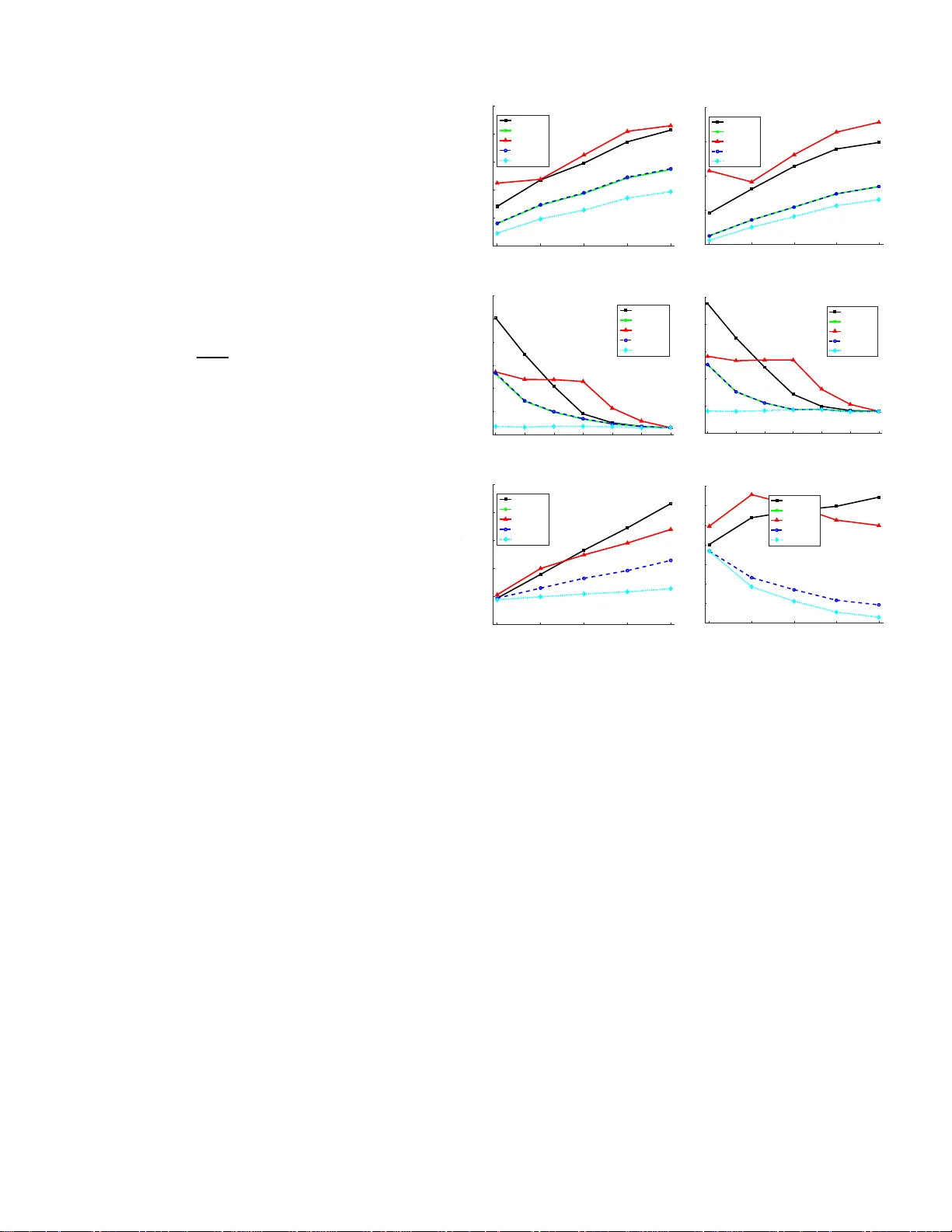
Sensing-Constrained LQG Control V asileios Tzoumas , 1 , 2 Luca Carlone , 2 George J. Pappas , 1 Ali Ja dbabaie 2 Abstract —Linear -Quadratic-Gaussian (LQG) control is con- cerned with th e design of an opt i mal controller an d estimator fo r linear Gaussian systems with imperfect state information. Standard L QG assumes th e set of sensor measurements, to b e fed to th e estimator , to be given. Howe ver , in many problems, arising in networked syste ms and robotics, one may not be able to use all the av ailable sensors, due to power or p ayload constraints, or may be interested in using the smallest subset of sen sors that guarantees the attainment of a desired control goal. In this paper , we introduce the sensing-constrained LQG c ontrol problem, in which one has to jointly design sensin g, estimation, and control, under giv en constraints on the resourc es spen t f or sensing. W e focus on th e realistic case i n whi ch the sensing strategy has to be selected among a fini te set of p ossib le sensing modalities. While the computation of the optimal sen si ng strategy is intractable, we present t he first scalable algorithm that computes a near - optimal sensing strategy with prova ble su b -optimality guarantees. T o this end, we show t h at a separation principle h old s, which allows the design of sensing, estimation, and control policies in isolation. W e conclu de the paper by discussing two applications of sensing-constrained LQG control, namely , sensing-constrained formation control and reso urce-constrained robo t navigation . This p aper has been accep ted for publication in th e IEEE Transactions of Au tomatic Con trol. Please cite the p aper as: V . T zoumas, L. Carlo ne, Geo rge J. Pappas, A. Jadb abaie “LQG Control an d Sensing Co-Design", IE E E Transactions o f Automatic Con tr ol (T A C), 202 0. I . I N T R O D U C T I O N T raditiona l approac hes to contro l of systems with partially observable state assume th e choice of sensors used to obser ve the system is g iv en. The ch oice of sen sors usually r esults fr om a p reliminary design phase in which an exper t d esigner selects a suitab le sensor suite th at accomm odates estimation req uire- ments (e.g., observability , d esired estimation erro r) a nd system constraints (e.g., size, cost). Moder n co n trol app lications, f rom large networked systems to miniaturize d ro botics systems, pose serious limitation s to the a pplicability of this traditional paradigm . In large-scale networked systems (e.g ., smart g rids or robot swarms), in which new nodes are continuously added and removed fro m the network, a m anual re-d esign o f the sensors becomes cu mbersome an d expen si ve, and it is simply not scalable. In miniatu rized r obot systems, while the set o f onboa r d sensors is fixed, it ma y be desirable to selecti vely activ ate on ly a subset of th e sensors du ring d ifferent phases of operation , in orde r to min imize power c o nsumptio n. In both application scenarios, one usually has access to a (po ssibly large) list of poten tial sen so rs, b ut, due to resource constraints 1 The authors are with the Department of Electrical and Systems Engi- neering , Unive rsity of Pennsylv ania, Philadelphia , P A 19104 USA (email: {pappagsg, vtzoumas}@seas.up enn.edu ). 2 The authors are with the Institute for Data, Systems and Society , and the Laboratory for Information and Decision Systems, Massachusetts In- stitute of T echnology , Cambridge, MA 02139 USA (email: {jadbabai, lcarlone, vtzoumas}@m it.edu ). This work was supported in part by T erraSw arm, one of six cente rs of ST ARnet, a Semiconductor Re search Corporation program sponsored by MARCO a nd D ARP A, and in part by AFOSR Comple x Net works Program. (e.g., cost, power), can only utilize a sub set of them. Mo reover , the need for online and large-scale sensor selection demands for auto mated approa c hes tha t efficiently select a sub set of sensors to maximize system performan ce. Motiv ated by these applications, in this paper we consider the prob lem of jointly design in g control, estimation, and sensor selection for a system with partially observable state. Related work. One body of related work is co ntr ol over band- limited communica tion channels , which inv estigates the trade-offs between com munication con straints ( e.g., data rate, quantization , delay s) an d control performance ( e . g., stability) in networked control systems. Early work p rovides results on the impact of qu antization [ 1], finite data rates [2], [3], and separation pr inciples for LQG design with commun ica- tion constrain ts [4]; more recent work focu ses o n p r iv acy constraints [5]. W e refer the read er to the surveys [6]–[8]. A seco nd set of r elated work is sensor selection and schedul- ing , in which o ne has to select a ( possibly time-varying ) set of sensors in order to monitor a pheno menon o f interest. Related literature inclu des appro aches based on rand omized sensor selection [9], dual volume sampling [10], [11], conve x relax- ations [12], [13], and subm odularity [14]–[16]. The third set of re la ted works is information-co nstrained (or informatio n- r e gularized) LQG contro l [17], [18]. Sh a fieepoorfard and Ra- ginsky [17] study rationa lly inattentiv e contro l laws for LQG control and discuss their effectiv eness in stabilizin g th e system. T anaka and Mitter [ 18] c onsider the co-design of sensing, control, an d estimation, propose to aug ment the stan d ard LQG cost with an informatio n -theore tic regularizer , an d der iv e an elegant solu tion based o n semidefinite p rogram ming. The main difference between our pr oposal a nd [1 8] is that we consider the case in which the choice of senso rs, rather than b eing arbitrary , is restricted to a finite set of available sen sors. Contributions. W e extend the Lin e ar-Quadratic-Gaussian (LQG) co ntrol to the case in which, besides d esigning an o p- timal con troller and estimator, one h as to select a set of sensors to be used to ob ser ve the system state. In particular, we fo r- mulate the sensing- constrained (finite-h o rizon) L Q G p roblem as the joint design of an optim al contr o l and estimation policy , as well as the selection o f a sub set of k out of N available sensors, that minimize the LQG ob jectiv e, which quantifies tracking perfor mance and co ntrol e ffort. W e first leverage a separation princ iple to show that the d esign of sen sing, contr ol, and estimation , can be perfo rmed in depend ently . While the computatio n of the optim al sensing strategy is combin atorial in nature, a key contribution of this pap er is to provid e the first scalable algo rithm that computes a ne ar-optimal sen sin g strategy with prov able sub-op tim ality guaran tees. W e moti vate the impo rtance of the sen sing-con stra in ed LQG p roblem, and demonstra te th e ef fectiveness of the prop osed a lg orithm in nu- merical exp eriments, by considerin g two applicatio n scen arios, namely , sensing- c o nstrained formation contr ol a nd r esource- constrained r obot navigation , which , due to page limitatio ns, we inclu d e in th e full version of this pap er , located at the authors’ websites. All p r oofs can b e foun d also in the full version of th is pap er , located at the authors’ websites. Notatio n. Lo wercase letters denote vectors and scalars, and upperc a se letters de n ote matr ices. W e use calligraphic fonts to denote sets. T he identity ma trix of size n is de n oted with I n (dimension is omitted when clear fro m th e co ntext). For a matrix M an d a vector v of approp riate dimension, we d efine k v k 2 M , v T M v . For ma trices M 1 , M 2 , . . . , M k , we define diag ( M 1 , M 2 , . . . , M k ) as the block diago nal m atrix with diagona l b lo cks the M 1 , M 2 , . . . , M k . I I . S E N S I N G - C O N S T R A I N E D L Q G C O N T RO L In this section w e forma lize th e sensing-co n strained LQG control pr oblem co n sidered in this paper . W e start by intro - ducing th e notions of system , sensors , and co ntr ol po licies . a) System: W e consider a standard discrete- tim e (po ssi- bly time-varying) lin ear system with additi ve Gaussian noise: x t +1 = A t x t + B t u t + w t , t = 1 , 2 , . . . , T , (1) where x t ∈ R n t represents the state o f the system at time t , u t ∈ R m t represents the c ontrol action , w t represents th e process no ise, and T is a finite time h orizon. In addition, we consider the system’ s initial condition x 1 to be a Gaussian random variable with covariance Σ 1 | 0 , and w t to be a Gaussian random v ariable with mean zero an d covariance W t , such that w t is indepen dent of x 1 and w t ′ for all t ′ = 1 , 2 , . . . , T , t ′ 6 = t . b) Sen sors: W e consider the c a se where we ha ve a (potentially large) set o f av ailable sensor s, wh ich take noisy linear o b servations o f the system’ s state. In particular , let V be a set of indice s such th at each in dex i ∈ V u niquely identifies a sensor that can be u sed to observe the state of the system. W e con sider sensors o f the f orm y i,t = C i,t x t + v i,t , i ∈ V , (2) where y i,t ∈ R p i,t represents the measuremen t o f sensor i at time t , and v i,t represents the measurem e n t noise of sensor i . W e assume v i,t to be a Gaussian random variable with mean zero an d po sitive definite covariance V i,t , such that v i,t is indepen d ent of x 1 , and of w t ′ for any t ′ 6 = t , and independent of v i ′ ,t ′ for all t ′ 6 = t , and a ny i ′ ∈ V , i ′ 6 = i . In th is pa per we ar e interested in the case in wh ich we cannot use all the a vailable sensors, and as a result, we need to select a convenient su bset of sensors in V to m a ximize our control pe r forman ce (fo rmalized in Problem 1 belo w). Definition 1 ( Active sensor set and mea surement model). Given a set of available sensors V , we say th at S ⊂ V is an activ e sensor set if we can observe the mea su r ements fr om ea ch sensor i ∈ S fo r all t = 1 , 2 , . . . , T . G iv e n an active sensor set S = { i 1 , i 2 . . . , i |S | } , we define the following qua ntities y t ( S ) , [ y T i 1 ,t , y T i 2 ,t , . . . , y T i |S | ,t ] T , C t ( S ) , [ C T i 1 ,t , C T i 2 ,t , . . . , C T i |S | ,t ] T , V t ( S ) , diag [ V i 1 ,t , V i 2 ,t , . . . , V i |S | ,t ] (3) which lead to the d e finition of the measur ement mod e l : y t ( S ) = C t ( S ) x t + v t ( S ) (4) wher e v t ( S ) is a zer o-mean Gaussian noise with covari- ance V t ( S ) . Despite the a vailability o f a possibly lar ge set of sensors V , our observer will only ha ve access to the measur ements p r o duced by the active sensors . The following p a ragraph formalizes how th e choice of the activ e sensor s affects th e c ontrol po licies. c) Contr ol policies: W e con sider co n trol p o licies u t for all t = 1 , 2 , . . . , T that ar e on ly inf ormed by the measuremen ts collected b y the acti ve sensors: u t = u t ( S ) = u t ( y 1 ( S ) , y 2 ( S ) , . . . , y t ( S )) , t = 1 , 2 , . . . , T . Such p o licies are called admissible . In th is p aper, we want to find a sm all set of active sensors S , and ad missible c ontroller s u 1 ( S ) , u 2 ( S ) , . . . , u T ( S ) , to solve the following sensing- constrained LQG control pro blem. Problem 1 ( Sensing- c onstrained LQG co ntrol). F ind a sen- sor set S ⊂ V o f cardinality at most k to be active a c r o ss all times t = 1 , 2 , . . . , T , and contr o l p olicies u 1: T ( S ) , { u 1 ( S ) , u 2 ( S ) , . . . , u T ( S ) } , that minimize the LQG co st fun ction: min S ⊆ V , |S |≤ k , u 1: T ( S ) T X t =1 E  k x t +1 ( S ) k 2 Q t + k u t ( S ) k 2 R t  , (5) wher e the state-co st ma trices Q 1 , Q 2 , . . . , Q T ar e positive semi-definite, the contr ol-cost matrices R 1 , R 2 , . . . , R T ar e positive defin ite, and the expectation is taken with r espect to the in itial condition x 1 , the pr ocess noises w 1 , w 2 , . . . , w T , and the measur ement n o ises v 1 ( S ) , v 2 ( S ) , . . . , v T ( S ) . Problem 1 generalizes the imperfect state-information LQG control pr oblem fro m the c ase whe re all sensors in V a r e activ e, an d on ly optim al contr ol policies are to be fou n d [19, Chapter 5], to the case whe r e only a few sensors in V can be active, and both optimal sensors and contro l policies are to be fo und jointly . While we alrea d y noticed th a t admissible control policies d epend on the active sensor set S , it is worth noticing that this in turn implies that the state ev olution also depend s on S ; for th is reason we write x t +1 ( S ) in eq. (5). The intertwinin g between co ntrol and sen sing calls for a joint design strategy . In the following sectio n we focus on the design of a jointly optimal con trol and sensing solution to Problem 1. I I I . J O I N T S E N S I N G A N D C O N T RO L D E S I G N In th is section we first presen t a separatio n pr inciple that de- couples sensing, estimation, and control, an d allo ws designing them in cascade (Section III- A). W e then present a scalable algorithm f o r sensing and con trol design (Section II I-B). Algorithm 1 Joint Sen sing and Control desig n for Prob lem 1. Input: Time horizon T , av ailable sen sor set V , covariance matrix Σ 1 | 0 of initial condition x 1 ; for all t = 1 , 2 , . . . , T , system m atrix A t , in put ma trix B t , LQG cost matrices Q t and R t , pro cess noise covariance matrix W t ; and f or all sensors i ∈ V , measurem ent matrix C i,t , and measuremen t noise covariance matrix V i,t . Output: Active sen sors b S , and contro l matrices K 1 , . . . , K T . 1: b S is retur n ed by Alg orithm 2 that finds a (p ossibly appr ox- imate) solu tio n to the optim ization prob lem in eq . (6); 2: K 1 , . . . , K T are computed u sing the recursion in eq. (8). A. Sep arability o f Optimal Sensing and Co n tr o l Desig n W e character ize the jointly optim a l co ntrol and sensing solutions to Prob lem 1, and pr ove that they can be fo und in two separate steps, where first the sensing design is computed, and second the correspond ing optimal co ntrol d esign is fou nd. Theorem 1 (Separ ability of opt ima l sensing and control de- sign). Let the sensor set S ⋆ and the co ntr ollers u ⋆ 1 , u ⋆ 2 , . . . , u ⋆ T be a solutio n to the sensin g -constrained LQG Pr oblem 1. Then, S ⋆ and u ⋆ 1 , u ⋆ 2 , . . . , u ⋆ T can be co mputed in casca de as fo llows: S ⋆ ∈ arg min S ⊆ V , |S |≤ k T X t =1 tr [Θ t Σ t | t ( S )] , (6) u ⋆ t = K t ˆ x t, S ⋆ , t = 1 , . . . , T (7) wher e ˆ x t ( S ) is the Kalman estimator of the state x t , i.e., ˆ x t ( S ) , E ( x t | y 1 ( S ) , y 2 ( S ) , . . . , y t ( S )) , and Σ t | t ( S ) is ˆ x t ( S ) ’s err or covariance, i.e., Σ t | t ( S ) , E [( ˆ x t ( S ) − x t )( ˆ x t ( S ) − x t ) T ] [19, Appen dix E]. In addition, the matrices Θ t and K t ar e in depend ent of the selected sensor set S , a nd they ar e compu te d as follows: the matrices Θ t and K t ar e the solution of the backwar d Riccati recurs ion S t = Q t + N t +1 , N t = A T t ( S − 1 t + B t R − 1 t B T t ) − 1 A t , M t = B T t S t B t + R t , K t = − M − 1 t B T t S t A t , Θ t = K T t M t K t , (8) with b o unda ry cond ition N T +1 = 0 . Remark 1 ( Certainty equivalence principle). The contr ol gain m a trices K 1 , K 2 , . . . , K T ar e th e same as the ones tha t make the co ntr ollers ( K 1 x 1 , K 1 x 2 , . . . , K T x T ) o ptimal for the perfect state-information version of P r o blem 1, wher e the state x t is kno wn to the contr ollers [19, Chapter 4]. Theorem 1 deco uples the d esign of the sen sing fro m the controller design. Moreover , it sugg e sts that once an optimal sensor set S ⋆ is fo u nd, then th e optim al contro llers are equ al to K t ˆ x t ( S ) , whic h corr e spond to the standar d LQG contr ol policy . This should not come as a surprise, since f or a given sensing strategy , Problem 1 reduce s to stand ard LQG con trol. W e co nclude this section with a remark providing a mor e intuitive interp retation of the sensor d esign step in eq. (6). Algorithm 2 Sensing design for Problem 1. Input: T ime hor izo n T , av ailable sensor set V , covariance matrix Σ 1 | 0 of system ’ s initial con dition x 1 , and for any time t = 1 , 2 , . . . , T , any sen sor i ∈ V , process noise covariance m a tr ix W t , measu rement matrix C i,t , and measuremen t n oise covariance matr ix V i,t . Output: Sensor set b S . 1: Compu te Θ 1 , Θ 2 , . . . , Θ T using r e cursion in eq. (8); 2: b S ← ∅ ; i ← 0 ; 3: while i < k do 4: for a ll a ∈ V \ b S do 5: b S a ← b S ∪ { a } ; Σ 1 | 0 ( b S a ) ← Σ 1 | 0 ; 6: for a ll t = 1 , . . . , T do 7: Σ t | t ( b S a ) ← 8: [Σ t | t − 1 ( b S a ) − 1 + C t ( b S a ) T V t ( b S a ) − 1 C t ( b S a )] − 1 ; 9: Σ t +1 | t ( b S a ) ← A t Σ t | t ( b S a ) A T t + W t ; 10: end for 11: cost a ← P T t =1 tr [Θ t Σ t | t ( b S a )] ; 12: end for 13: a i ← a r g min a ∈V \S cost a ; 14: b S ← b S ∪ { a i } ; i ← i + 1 ; 15: end while Remark 2 (Co ntrol-aware sensor design). In order to pr o- vide mor e in sig h t on the cost function in ( 6) , we re write it as: T X t =1 tr [Θ t Σ t | t ( S )] = T X t =1 E  tr { [ x t − ˆ x t ( S )] T Θ t [ x t − ˆ x t ( S )] }  = T X t =1 E  k K t x t − K t ˆ x t ( S ) k 2 M t  , (9) wher e in the first line we used th e fact that Σ t | t ( S ) = E  ( x t − ˆ x t ( S ))( x t − ˆ x t ( S )) T  , and in the second line we substituted th e defin ition of Θ t = K T t M t K t fr o m eq. (8) . F r om eq. (9) , it is clear th at each term tr [Θ t Σ t | t ( S )] captures the expected contr ol mismatch between the imperfect state-information contr oller u t ( S ) = K t ˆ x t ( S ) ( which is only awar e of the measurements fr om the active sen sors) and the perfect state-information contr oller K t x t . This is an important distinction fr om the existing sensor selection literatur e. In p ar- ticular , while stan dar d sensor selection attempts to min imize the estimation covariance, for instance by minimizing T X t =1 tr [Σ t | t ( S )] , T X t =1 E  k x t − ˆ x t ( S ) k 2 2  , (10) the pr o posed LQG cost formulation a ttempts to minimize the estimation e rr or of only the in formative state s to th e perfect state-information con tr o ller: for example, the contribution of all x t − ˆ x t ( S ) in the null space o f K t to th e total contr ol mismatch in eq. (9) is zer o . Hence, in contrast to minimizing the cost fu n ction in eq . (10) , minimizing the co st function in eq. (9) r esults to a contr ol-aware sensing design. B. Sca lable Near-optimal Sensin g and Contr ol Design This section p r oposes a practical design algorithm f or Problem 1. The pseudo-c ode of the alg orithm is presen ted in Algorithm 1. Algorithm 1 follows the result o f Theo r em 1, and jointly designs sensin g and contro l b y first computin g an activ e sensor set (line 1 in Algo rithm 1) an d then com puting the control policy (line 2 in Algorithm 1) . W e discuss each step o f the design proc e ss in the rest of this sectio n. 1) Near-optimal Sen sin g design: T h e op timal senso r design can be computed b y solv in g the optim ization pro blem in eq. (6). The pr o blem is comb inatorial in n ature, since it requires to select a su b set of elemen ts of cardinality k ou t of all the available sen so rs that induces the smallest cost. In this section we p ropo se a greedy algorithm , whose pseudo- c ode is giv en in Algor ithm 2, that c omputes a ( possibly approx imate) solu tion to the p roblem in eq. (6). Ou r interest tow ards this gre e d y algorithm is motiv ated by the fact that it is scalable (in Section IV we show that its co m plexity is linear in the number o f available senso rs) and is pr ovably close to the optimal solutio n of the pr oblem in eq. (6 ) (we provide subop timality boun ds in Section IV). Algorithm 2 co m putes the m a trices Θ t ( t = 1 , 2 , . . . , T ) which ap pear in th e c o st functio n in eq. (6) (line 1). Note that these m a tr ices are indepen dent on the ch o ice of sensors. The set of active sensors b S is in itialized to the empty set (line 2) . Th e “while lo op” in line 3 will be executed k times and at each time a sensor is greedily added to th e set of ac tive senso r s b S . I n particu lar , th e “for loop ” in lines 4-1 2 com putes the e stima tio n covariance resulting by adding a sensor to th e current activ e sensor set and the correspo nding cost (line 11). Finally , the sensor inducing the smallest cost is selected (line 13) a n d added to th e curr ent set of active sensor s (line 14). 2) Contr ol po licy design : The optimal contro l design is computed as in eq. (7), where the contro l p olicy matrices K 1 , K 2 , . . . , K T are ob tained from the recur sio n in eq. (8). In the fo llowing section we characterize the a p prox im ation and r u nning -time pe rforma n ce of Alg orithm 1. I V . P E R F O R M A N C E G U A R A N T E E S F O R J O I N T S E N S I N G A N D C O N T RO L D E S I G N W e prove that Algorith m 1 is the first scalable algo rithm for the join t sensing an d control design Pro blem 1, and tha t it achieves a value for the LQG cost functio n in eq. (5) that is finitely close to the optimal. W e start by introd u cing the notion of superm o dularity ratio (Sectio n IV -A), which will en able to bound the sub -optimality g ap of Alg orithm 1 (Section I V - B). A. Sup ermodula rity ratio of monotone func tions W e define the supermod ularity ratio of m onoto n e function s. W e start with the notio ns o f mono tonicity and su permod ularity . Definition 2 (Monotonicit y [20]). Conside r an y finite gr ou nd set V . The set fun ction f : 2 V 7→ R is non-in cr easing if and only if for an y A ⊆ A ′ ⊆ V , f ( A ) ≥ f ( A ′ ) . Definition 3 (Supermodularity [20, Proposition 2.1]). Con- sider a n y finite g r o und set V . The set function f : 2 V 7→ R is supermodula r if and o nly if for any A ⊆ A ′ ⊆ V an d x ∈ V , f ( A ) − f ( A ∪ { x } ) ≥ f ( A ′ ) − f ( A ′ ∪ { x } ) . In words, a set fun c tio n f is super modular if and on ly if it satisfies th e following intu itive diminishin g returns pr operty: for any x ∈ V , the marginal drop f ( A ) − f ( A ∪ { x } ) diminishes as A grows; equivalently , for a ny A ⊆ V and x ∈ V , the marginal drop f ( A ) − f ( A ∪ { x } ) is non-in creasing. Definition 4 (Supermodularity r a tio [21, Definition of elemental curvature on p. 5] ). Consider any fin ite gr ound set V , an d a non-increasing set function f : 2 V 7→ R . W e define the supermodula rity ratio o f f as γ f = min A⊆V ,x,x ′ ∈V \A f ( A ) − f ( A ∪ { x } ) f ( A ∪ { x ′ } ) − f [( A ∪ { x ′ } ) ∪ { x } ] . In words, the superm odularity r atio of a mo noton e set function f m easures h ow far f is fr o m b eing su permod ular . In particular , per the Definitio n 4 of super modular ity ra tio , the supermod ularity ratio γ f takes values in [0 , 1 ] , and • γ f = 1 if and only if f is su permod ular, since if γ f = 1 , then Definition 4 implies f ( A ) − f ( A ∪ { x } ) ≥ f ( A ∪ { x ′ } ) − f [( A ∪ { x ′ } ) ∪ { x } ] , i.e., the dr o p f ( A ) − f ( A ∪ { x } ) is non-incr easing as new elemen ts are added in A . • γ f < 1 if and only if f is ap pr oximately supermodu lar , in the sense that if γ f < 1 , then Definition 4 im p lies f ( A ) − f ( A ∪ { x } ) ≥ γ f { f ( A ∪ { x ′ } ) − f [( A ∪ { x ′ } ) ∪ { x } ] } , i.e., the drop f ( A ) − f ( A ∪ { x } ) is app roximately non - increasing as new elements are ad ded in A ; specifically , the supermo dularity ra tio γ f captures how m uch ones needs to discou nt the drop f ( A ∪ { x ′ } ) − f [( A ∪ { x ′ } ) ∪ { x } ] , such that f ( A ) − f ( A ∪ { x } ) remains gre a ter then, or eq u al to, f ( A ∪ { x ′ } ) − f [( A ∪ { x ′ } ) ∪ { x } ] . W e n ext use the notion o f supermod ularity r atio Defin ition 4 to qua ntify the sub-optimality gap of Algorithm 1. B. P erformance Analysis fo r Alg orithm 1 W e qua ntify Algo rithm 1’ s runnin g time, as well as, Al- gorithm 1’ s approx im ation per f ormanc e, using the n otion of supermod ularity r atio introdu ced in Section IV -A. W e co n- clude the section by showing that fo r app ropriate L QG cost matrices Q 1 , Q 2 , . . . , Q T and R 1 , R 2 , . . . , R T , Algo r ithm 1 achieves near-optimal appro ximate p erform ance. Theorem 2 (Performance of Algorithm 1). F or a ny active sensor set S ⊆ V , and admissible contr ol po licies u 1: T ( S ) , { u 1 ( S ) , u 2 ( S ) , . . . , u T ( S ) } , let h [ S , u 1: T ( S )] be Pr o blem 1’s cost fu nction, i.e., h [ S , u 1: T ( S )] , P T t =1 E ( k x t +1 ( S ) k 2 Q t + k u t ( S ) k 2 R t ); Further define the following set-valued function an d scalar: g ( S ) , min u 1: T ( S ) h [ S , u 1: T ( S )] , (11) g ⋆ , min S ⊆ V , |S |≤ k , u 1: T ( S ) h [ S , u 1: T ( S )] . The following results hold true: 1) (Appr oximatio n qua lity) Algorithm 1 returns an active sensor set b S ⊂ V of cardinality k , and gain matrices K 1 , K 2 , . . . , K T , such that the cost h [ b S , u 1: T ( b S )] attained by the sensor set b S and the corr espond ing contr ol policies u 1: T ( b S ) , { K 1 ˆ x 1 ( b S ) , . . . , K T ˆ x T ( b S ) } satisfies h ( b S , u 1: T ( b S )) − g ⋆ g ( ∅ ) − g ⋆ ≤ exp( − γ g ) (12) wher e γ g is the supermodularity ratio of g ( S ) in eq . (11) . 2) (Runn ing time) Algo rithm 1 runs in O ( k |V | T n 2 . 4 ) time, wher e n , max t =1 , 2 ,...,T ( n t ) is the maximum system size in e q. (1) . Theorem 2 ensures that Algorithm 1 is th e first scalab le algorithm f o r the sensing-constra ined LQG control Problem 1. In particular , Algorithm 1’ s running time O ( k |V | T n 2 . 4 ) is lin- ear both in the number o f av ailable sensors |V | , and the sensor set car dinality con straint k , as w e ll as, line a r in the Kalman filter’ s r unning time across the time ho r izon { 1 , 2 . . . , T } . Specifically , the contribution n 2 . 4 T in Algo rithm 1 ’ s ru n ning time com es f rom the compu tational com p lexity of u sing the Kalman filter to comp ute the state estimation er ror covariances Σ t | t for ea c h t = 1 , 2 , . . . , T [19, Appendix E ]. Theorem 2 also guaran tees that for non- z ero ratio γ g Algorithm 1 achieves a value for Pro blem 1 that is finitely close to the op timal. In particu lar , the bound in ineq . (1 2) improves as γ g increases, sinc e it is d ecreasing in γ g , and is char a c terized by the fo llowing extreme behaviors: f or γ g = 1 , the boun d in ineq. (1 2) is e − 1 ≃ . 37 , which is th e minim u m for any γ g ∈ [0 , 1] , and h ence, the best bound on Algorithm 1’ s app roximatio n per forman ce among all γ g ∈ [0 , 1] (ide a lly , the bou nd in ineq. (12) would be 0 for γ g = 1 , in which case Algorithm 1 would be exact, since it would be implied h ( b S , u 1: T ( b S )) = g ⋆ ; h owever , ev en f or sup ermod u lar fun ctions, the best bound on e can achieve in the worst-case is e − 1 [22]); for γ g = 0 , ineq. (12) is uninformative since it simplifies to h ( b S , u 1: T ( b S )) ≤ g ( ∅ ) = h ( ∅ , u 1: T ( ∅ )) , wh ich is trivially satisfied. 1 In the rem aining of the sectio n, we first prove th at if the strict ine q uality P T t =1 Θ t ≻ 0 holds, whe r e each Θ t is defined as in eq. (8), then the ratio γ g in ineq. (12) is non -zero, and as result Algorithm 1 achieves a near-optimal approx imation perfor mance (Th e orem 3). Then, we pr ove th at the strict inequality P T t =1 Θ t ≻ 0 holds tru e in all LQG contro l pr oblem instances where a zero con troller would result in a suboptimal behavior of the system and, as a re sult, LQG contro l design (throu g h solving Prob lem 1 ) is necessary to ach iev e th eir desired sy stem perfor mance (Th eorem 4). Theorem 3 (Lower bound for supermodularity r atio γ g ). Let Θ t for all t = 1 , 2 , . . . , T be de fined as in eq. ( 8) , g ( S ) 1 The inequalit y h ( b S , u 1: T ( b S )) ≤ h ( ∅ , u 1: T ( ∅ )) simply states that a con- trol polic y that is in formed by the acti ve sensor set S has better performance than a pol icy t hat doe s not use any sensor; for a more formal proof we refer the reader to Appendix B. be d e fi ned as in eq. (1 1) , an d for a n y sensor i ∈ V , ¯ C i,t be the no rmalized measurement matrix V − 1 / 2 i,t C i,t . If P T t =1 Θ t ≻ 0 , the supermodularity r atio γ g is non-zer o. In a d dition, if we conside r for simplicity that the F r ob enius norm of each ¯ C i,t is 1 , i.e., tr  ¯ C i,t ¯ C T i,t  = 1 , and that tr [Σ t | t ( ∅ )] ≤ λ 2 max [Σ t | t ( ∅ )] , γ g ’ s lower bound is γ g ≥ λ min ( P T t =1 Θ t ) λ max ( P T t =1 Θ t ) min t ∈{ 1 , 2 ,...,T } λ 2 min [Σ t | t ( V )] max t ∈{ 1 , 2 ,...,T } λ 2 max [Σ t | t ( ∅ )] 1 + min i ∈V ,t ∈{ 1 , 2 ...,T } λ min [ ¯ C i Σ t | t ( V ) ¯ C T i ] 2 + max i ∈V ,t ∈{ 1 , 2 ...,T } λ max [ ¯ C i Σ t | t ( ∅ ) ¯ C T i ] . (13) The supermod ularity r atio boun d in ineq. (13) suggests two cases und er which γ g can in c rease, and co rrespon dingly , th e perfor mance bou nd of Algorithm 1 in eq. (12) can imp rove: a) Case 1 wher e γ g ’ s bound in ineq. (13) increases: When the f raction λ min ( P T t =1 Θ t ) /λ max ( P T t =1 Θ t ) inc r eases to 1 , th en th e r ight-han d-side in ine q. (13) incre ases. Equ iv- alently , the r ig ht-han d -side in ineq. (13) incr eases when on av erage all th e directions x ( i ) t − ˆ x ( i ) t of the estimation errors x t − ˆ x t = ( x (1) t − ˆ x (1) t , x (2) t − ˆ x (2) t , . . . , x ( n t ) t − ˆ x ( n t ) t ) b e c ome equally imp ortant in selecting the active sensor set. T o see this, consider fo r example that λ max (Θ t ) = λ min (Θ t ) = λ ; th e n, the co st function in eq. (6) that A lg orithm 1 minimize s to select the acti ve sensor set beco m es T X t =1 tr [Θ t Σ t | t ( S )] = λ T X t =1 E  tr ( k x t − ˆ x t ( S ) k 2 2 )  = λ T X t =1 n t X i =1 E h tr ( k x ( i ) t − ˆ x ( i ) t ( S ) | 2 2 ) i . Overall, it is easier fo r Algorithm 1 to appro ximate a solution to Problem 1 as the co st functio n in eq. (6) becomes th e c ost function in th e standar d sensor selectio n problems wher e o ne minimizes th e total estimation cov ariance as in eq. ( 1 0). b) Case 2 wher e γ g ’ s bound in ineq. (13) increases: When either the numerato rs of the last two fractions in the right-ha n d-side of ineq. (13) inc rease or the d enomin ators of the last two fractions in the r ight-han d-side of ineq. (13) decrease, then the r ight-han d-side in ineq. (13) inc reases. In particu lar, the numerato rs of the last two fraction s in right- hand-side of ineq. (13) capture the estimation qu ality when all available sensors in V are used, v ia the terms o f the form λ min [Σ t | t ( V )] and λ min [ ¯ C i,t Σ t | t ( V ) ¯ C T i,t ] . Interestingly , this sug gests th at the righ t-hand- side of ineq. (13) increases when the avail able sensors in V are inefficient in achieving low e stima tion erro r , that is, wh en the terms of the f orm λ min [Σ t | t ( V )] and λ min [ ¯ C i,t Σ t | t ( V ) ¯ C T i,t ] in crease. Sim ilar ly , the de n ominato rs o f the last two fra c tio ns in right-han d- side of ineq. (13) cap ture the estimatio n quality when n o sensors are u sed, via the ter ms o f the fo rm λ max [Σ t | t ( ∅ )] an d λ max [ ¯ C i,t Σ t | t ( ∅ ) ¯ C T i,t ] . This suggests that the right-h and-side of ineq. ( 13) incre a ses when th e m easuremen t noise increases. W e next give a control-level eq uiv alent con dition to Th eo- rem 3’ s co ndition P T t =1 Θ t ≻ 0 fo r no n-zero ratio γ g . -9 -8 -7 -6 -5 -4 -3 -2 -1 0 1 2 3 4 5 6 7 8 9 x [meters] -9 -8 -7 -6 -5 -4 -3 -2 -1 0 1 2 3 4 5 6 7 8 9 y [meters] (a) formation control (b) u nmann e d aerial robot Fig. 1. Examples of appl ications of th e propose d sensing-const rained L Q G control framewo rk: (a) sensing-const rained formation control and (b) resource- constrai ned robot na vigation . Theorem 4 (Control-level condition for near -optimal sensor selection). Con sider th e LQG pr o blem wher e for any time t = 1 , 2 , . . . , T , the state x t is known to each contr oller u t and the pr ocess no ise w t is zer o, i.e., the optimization pr oblem min u 1: T P T t =1 [ k x t +1 k 2 Q t + k u t ( x t ) k 2 R t ]   Σ t | t = W t =0 . (14) Let A t to b e in vertible for all t = 1 , 2 , . . . , T ; the strict inequality P T t =1 Θ t ≻ 0 hold s if and only if for all non-zer o initial con ditions x 1 , 0 / ∈ arg min u 1: T P T t =1 [ k x t +1 k 2 Q t + k u t ( x t ) k 2 R t ]   Σ t | t = W t =0 . Theorem 4 sugge sts that T heorem 3’ s sufficient cond ition P T t =1 Θ t ≻ 0 for no n-zero r atio γ g holds if a n d only if f o r any non -zero initial con dition x 1 the all-zeroes control policy u 1: T = (0 , 0 , . . . , 0) is subop timal fo r th e noiseless per fect state-inform ation LQ G problem in eq. (14). Overall, Algor ithm 1 is the fir st scalable alg orithm fo r Problem 1, and (fo r th e LQG contro l pr oblem in stances of interest where a zero contr oller would r esult in a suboptimal behavior of the system and, as a re sult, LQG contro l design is necessary to ach iev e th e ir desired system perfor mance) it achieves close to optimal approximate perfo r mance. V . N U M E R I C A L E X P E R I M E N T S W e consider two ap plication scenarios for the p ro- posed sensing- constrained LQG con trol framework: sensing- constrained fo rmation co ntr ol an d res ource-constrained r o bot navigatio n . W e pre sen t a Mon te Carlo analy sis for bo th scenar- ios, which d emonstrates that (i) th e pro posed sensor selection strategy is near-optima l, a n d in particular, the resulting LQG- cost (trac k ing perfor mance) matches the op timal selection in all tested instances for wh ic h the optimal selection could be compu ted via a brute-fo rce appr oach, (ii) a more naive selection which attempts to m in imize the state estimatio n covariance [1 5] (r ather than the LQG cost) has degraded L QG tracking perfo rmance, often com parable to a ran dom selectio n , (iii) in the considered instances, a clever selectio n of a small subset of senso r s can e n sure an LQG c ost that is close to the one obtained by using all av ailable senso r s, hen ce pr oviding an effecti ve alternative for control under sensin g con straints [ 23]. V I . S E N S I N G - C O N S T R A I N E D F O R M A T I O N C O N T RO L Simulation setup. Th e first applicatio n scenario is illus- trated in Fig . 1 (a). A team of n agen ts (b lue trian gles) moves in a 2D scen ario. At time t = 1 , the agen ts ar e rand omly deployed in a 10m × 10 m square and their objective is to reach a target fo r mation shape (red stars); in the example of Fig. 1(a) the desired fo rmation has an hexag onal shape, while in gen eral for a form ation of n , th e desired form a tion is an equilateral po lygon with n vertices. Each robo t is modeled as a double- in tegrator, with state x i = [ p i v i ] T ∈ R 4 ( p i is the 2 D position of agent i , while v i is its velocity), and can contro l its own acceleration u i ∈ R 2 ; th e process n oise is cho sen as a diagonal matrix W = diag  [1 e − 2 , 1 e − 2 , 1 e − 4 , 1 e − 4 ]  . Each ro bot i is equ ip ped with a GPS receiver , which can measure the agent p o sition p i with a covariance V gps,i = 2 · I 2 . Moreover , the agents are equipped with lidar sensors allowing each agent i to mea sure th e r e lati ve position of anoth er agent j with covariance V lidar,ij = 0 . 1 · I 2 . The agents have very limited on -board resources, hen ce they can o nly activ ate a subset of k sensor s. Hence, the goal is to select the subset o f k senso rs, as well as to com p ute the contr ol po licy that ensu re best trackin g perfo r mance, as measured by the LQG objec tive. For our tests, we consider two p roblem setups. In the first setup, n a med homogeneou s formation c ontr ol , the L QG we ig h matrix Q is a block diagonal matrix with 4 × 4 b locks, with each blo ck i cho sen as Q i = 0 . 1 · I 4 ; since each 4 × 4 block of Q we ig hts the tracking error of a robot, in the ho mogene o us case the trac k ing error o f all agents is equally impo rtant. In the seco nd setu p, named h eter ogeneous forma tio n contr ol , the matrix Q is chose as above, except for o ne of th e agen ts, say robo t 1 , for which we choo se Q 1 = 1 0 · I 4 ; this setup models the case in wh ich each agent h as a different role or importan ce, he n ce one weights differently the tr acking err or of the agen ts. In both cases the matrix R is c h osen to be the identity matrix. The simu lation is carried o n o ver T time steps, and T is also chosen as LQG h orizon. Results are av erage d over 100 Monte Carlo run s: at ea ch r un we ran d omize the initial estima tio n covariance Σ 1 | 0 . Compared techniques. W e com p are five techn iq ues. All technique s use an L Q G - based estimator and controller, a n d they only differ b y the selections of the sensors used. The first appr oach is the optimal sensor selection , denoted as optimal , which attains the minimum of the cost fu n ction in eq. ( 6), and that we com pute by enu m erating all possible subsets; this br ute-forc e approach is on ly v iable when the number of av ailable sensors is small. The second ap proach is a p seudo-r andom sen sor selectio n, d enoted as r andom ∗ , which selects all the GPS m easurements and a ran dom subset of th e lidar measurem ents; no te that we d o n o t con sider a fully rand om selectio n since in p ractice this often leads to an unobser vable system, henc e ca using d iv ergence of the LQG cost. The th ird appr oach, denoted as logdet , selects sensor s so to minimize the average log de t of the estimation c ovariance over the horizo n; this app r oach resembles [ 15] and is agn ostic to the control task. The fourth appro ach is the prop osed sensor selection strategy , described in Algo r ithm 2, and is de n oted as s-LQG . Finally , we also report th e L QG perfor mance when all sensors are selected. This approach is deno ted as allSensors . Results. The results of our numer ical analy sis a re rep o rted in Fig. 2. When not specified otherw ise, we co nsider a formation of n = 4 ag ents, which can only use a total of k = 6 sensors, and a contro l horizo n T = 20 . Fig. 2( a) shows the LQG cost attain ed by the comp ared technique s for increasing co ntrol horizon and for the homog eneou s case. W e note th a t, in all tested instance, the proposed appro ach s-LQG matches the optimal selection opti mal , and both appro aches are rela tively close to allSe nsors , which selects all the av ailable sen sors ( n + n 2 2 ). On the o ther hand logdet leads to worse track in g p erform ance, and it is often c lo se to the pseudo- r andom selection random ∗ . T hese consideratio ns are confirmed by the heterog eneous setup, shown in Fig. 2(b) . In this c a se the separ ation b etween the p roposed appr oach and logdet b ecomes even larger; the intu ition here is tha t the heterog eneous case rewards differently the trackin g err o rs at different ag ents, hence while logdet attempts to equally reduce the estimation error across the f ormation , the pro posed approa c h s-LQG selects sensors in a task-o riented fashion , since the matrices Θ t for all t = 1 , 2 , . . . , T in the cos t function in eq. ( 6) incorp orate the LQG weight matrices. Fig. 2( c) shows the LQG cost attained by the co mpared technique s f o r increasing num b er o f selected sensors k and for the homo geneou s case. W e note that for increasing num ber of sensors all techn iques converge to allSenso rs (the entire groun d set is selected). As in the previous case, the p ropo sed approa c h s-LQG ma tc h es the optima l selection optimal . Fig. 2(d) shows the same statistics for th e heterogeneo us case. W e no te that in this case logdet is inferior to s-LQG even in the case with small k . Moreover , an interesting fact is that s-LQG m a tches allSensors alr eady for k = 7 , meaning that the LQG p erform a nce of the sensin g -constrain t setup is indistinguishab le fro m the o ne using all sensors; in tuitiv ely , in the heterog eneous case, ad d ing m o re sensors may have marginal impact on the LQG cost (e.g ., if the cost rewards a small tra cking erro r fo r rob ot 1, it m ay be of little value to take a lidar measureme nt betwe e n rob ot 3 an d 4). This further stresses the impo rtance of th e p roposed framework as a parsimonio us way to control a system with minimal resour ces. Fig. 2(e) and Fig. 2(f) show the LQ G c ost attained by the compare d techniq u es f or increasing number of agents, in the homog eneous and heterogeneou s case, respecti vely . T o ensure observability , we consider k = r ound (1 . 5 n ) , i.e., we select a number of sensors 50% larger than the smallest set of sensors that can make the sy stem obser vable. W e note that optimal quickly becom es in tractable to c o mpute, hence we omit values beyond n = 4 . In b oth figures, the ma in observation is that the separation among the tech niques increases with the n umber of ag e nts, since the set of available sen sors q uickly incr eases with n . I n terestingly , in the heter ogeneo us case s -LQG re- mains relatively clo se to allSenso rs , implying that for th e purpo se of LQG control, using a cle verly selected small sub set 10 15 20 25 30 horizon 2 4 6 8 10 12 LQG cost random * optima l logdet s-LQG allSens ors (a) ho mogen eous 10 15 20 25 30 horizon 50 100 150 200 250 LQG cost random * optimal logdet s-LQG allSenso rs (b) h eterogen eous 4 5 6 7 8 9 10 maxNrUsedSensors 4 6 8 10 12 14 16 LQG cost random * optimal logdet s-LQG allSenso rs (c) ho mogen eous 4 5 6 7 8 9 10 maxNrUsedSensors 50 100 150 200 250 300 LQG cost random * optimal logdet s-LQG allSenso rs (d) h eterogen eous 3 5 7 9 11 nrRobots 0 5 10 15 20 25 LQG cost random * optima l logdet s-LQG allSens ors (e) ho mogen eous 3 5 7 9 11 nrRobots 40 60 80 100 120 140 160 180 LQG cost random * optimal logdet s-LQG allSenso rs (f) h eterogen eous Fig. 2. LQG cost for increasin g (a )-(b) control horizon T , (c)-(d) number of select ed sensors k , and (e)-(f) number of ag ents n . Stat istics are re ported for the homogeneous formation control setup (left column), and the heterogen eous setup (right column). Results are ave raged ov er 100 Monte Carlo runs. of sensor s still ensures excellent trac k ing perf ormance . V I I . R E S O U R C E - C O N S T R A I N E D RO B OT N A V I G A T I O N Simulation setup. The second app lica tion scenario is illus- trated in Fig. 1(b). An unm anned aer ial rob ot (UA V) moves in a 3 D scenario, starting from a rando mly selected initial location. The objectiv e of the U A V is to land, an d more specifically , it has to reach the po sition [0 , 0 , 0] with zero velocity . Th e UA V is mo deled as a d ouble- integrator, with state x i = [ p i v i ] T ∈ R 6 ( p i is the 3D p osition o f agent i , while v i is its velocity ), and can control its own ac c eleration u i ∈ R 3 ; th e pro cess noise is chosen as W = I 6 . The UA V is equip p ed with multiple sensor s. It has an on-b oard G PS receiver , measur in g the U A V position p i with a c ovariance 2 · I 3 , an d an altimeter, measu ring only the last co mpone n t of p i (altitude) with stand ard deviation 0 . 5m . Moreover, the U A V can u se a stereo camera to measur e th e relativ e position of ℓ landmark s o n the g round ; f or the sake of the n umerical example, we assume th e lo cation of each landma rk to be known only approximately , and we associate to each land mark an u n certainty covariance (r e d ellipsoids in Fig. 1(b)), which is 10 20 30 40 50 horizon 90 100 110 120 130 LQG cost / T random * optimal logdet s-LQG allSenso rs (a) ho mogen eous 4 6 8 10 12 maxNrUsedSensors 2250 2300 2350 2400 2450 2500 LQG cost random * optimal logdet s-LQG allSenso rs (b) h eterogen eous Fig. 3. LQG cost for increasin g (a) control horizon T , and (b) number of select ed sensors k . Statistic s are reported for the heterogeneou s setu p. Results are avera ged ove r 100 Monte Carlo runs. random ly gen e rated at the beginning of each run. Th e U A V h a s limited on-boar d resources, hence it can only activ ate a subset of k sensors. For instance, the resou rce-con straints m ay b e due to the power consump tion o f the GPS an d the altime ter , or may be du e to com putational co nstraints that prevent to run multiple ob je c t-detection algorithms to detect all landmar ks on the grou nd. Similarly to the previous case, we ph r ase the problem as a sensing-con stra int LQG pro blem, an d we use Q = diag  [1 e − 3 , 1 e − 3 , 10 , 1 e − 3 , 1 e − 3 , 10 ]  and R = I 3 . Note that th e structur e of Q reflects the fact that du ring landing we are pa r ticularly interested in controlling the vertical direction and the vertical v elocity (entries with larger weigh t in Q ), while we are less inter ested in co ntrolling accur ately th e horizon tal position and velocity (assum in g a sufficiently large landing site). In the fo llowing, we presen t r esults averaged over 100 Monte Carlo runs: in each run, we rand omize th e covariances describ ing the lan dmark p o sition uncerta in ty . Compared tec hniques. W e co nsider the five techn iques discussed in the previous section. As in the for mation con trol case, the pseudo-ra ndom selection random ∗ always inclu des the GPS measurement (which alone en sures obser vability) and a r a ndom selection of the other av ailable sensor s. Results. The results of our numer ical analy sis a re rep o rted in Fig . 3 . When not specified other wise, we consider a total of k = 3 senso r s to be selected, and a contr ol h orizon T = 20 . Fig. 3(a) shows the LQG cost attained by the com pared technique s fo r incr e asing contro l ho rizon. For visualization purpo ses we plot the cost norm alized by the hor izon, which makes more visible the difference s among the techniqu es. Sim- ilarly to th e formatio n co n trol example, s -LQG matches the optimal selection o ptimal , while logdet a n d random ∗ have subo ptimal perfo rmance. Fig. 3(b) shows the LQG co st attained b y the compared technique s for increa sin g numbe r of selected sensors k . Clearly , all techniques con verge to allSensors for increas- ing k , but in the regime in which few sen so rs ar e u sed s -LQG still outperfo r ms alternative sensor selection schemes, and matches in all cases the o p timal selection optimal . V I I I . C O N C L U D I N G R E M A R K S In th is p a p er , we intro duced the sensing- constrained LQG contr ol Problem 1, which is c e ntral in moder n con trol a p - plications that r ange fr om large-scale n etworked systems to miniaturized robo tics networks. While the computation of the optima l sensing strategy is intractable, W e provided th e first scalab le algorithm for Pro blem 1 , Algorithm 1 , and under mild condition s o n the system and LQG m atrices, proved that Alg orithm 1 computes a near-optimal sensing strategy with provable sub-optimality guar antees. T o this end, we showed that a separa tion principle holds, which allo ws the design o f sensing, estimation, and control policies in isolation. W e motiv ated the importance of the sensing- constrained LQG Problem 1, and dem onstrated th e effecti veness of Algor ithm 1, by conside r ing two application scenarios: sensing-con strained formation con tr o l , and resour ce-constrained r obot naviga tion . A P P E N D I X A : P R E L I M I N A RY FAC T S This appen d ix con tains a set of lemmata that will be used to supp ort the proofs in this paper ( Append ices B–F). Lemma 1 ([24, Proposition 8.5.5] ). Consider two positive definite matrices M 1 and M 2 . If M 1  M 2 then M − 1 2  M − 1 1 . Lemma 2 (T race inequality [24, Propositio n 8 . 4.13] ). Con- sider a symmetric matrix A , an d a po sitive semi-d efinite matrix B o f a ppr opriate dimension . Then, λ min ( A ) tr ( B ) ≤ tr ( AB ) ≤ λ max ( A ) tr ( B ) . Lemma 3 (W o odbury identity [24, Corollar y 2.8.8 ]). Co n - sider ma trices A , C , U and V of appr opriate dimensions, su ch that A , C , and A + U C V ar e in v ertible. Then, ( A + U C V ) − 1 = A − 1 − A − 1 U ( C − 1 + V A − 1 U ) − 1 V A − 1 . Lemma 4 ([24, Proposition 8. 5 .12]) . Consider two symmetric matrices A 1 and A 2 , and a positive semi-d efinite matrix B . If A 1  A 2 , th en tr ( A 1 B ) ≤ tr ( A 2 B ) . Lemma 5 ([19, A ppendix E]). F or any sensor set S ⊆ V , and for a ll t = 1 , 2 , . . . , T , let ˆ x t ( S ) be the Kalman estimator of the state x t , i.e., ˆ x t ( S ) , a nd Σ t | t ( S ) b e ˆ x t ( S ) ’s err o r covariance, i.e., Σ t | t ( S ) , E [( ˆ x t ( S ) − x t )( ˆ x t ( S ) − x t ) T ] . Then, Σ t | t ( S ) is the solution of th e Kalman fi ltering r ecursion Σ t | t ( S ) = [Σ t | t − 1 ( S ) − 1 + C t ( S ) T V t ( S ) − 1 C t ( S )] − 1 , Σ t +1 | t ( S ) = A t Σ t | t ( S ) A T t + W t , (15) with b o unda ry cond ition the Σ 1 | 0 ( S ) = Σ 1 | 0 . Lemma 6. F or an y sensor set S ⊆ V , let Σ 1 | 1 ( S ) be defined as in eq. ( 1 5) , an d consider two sen sor sets S 1 , S 2 ⊆ V . If S 1 ⊆ S 2 , th en Σ 1 | 1 ( S 1 )  Σ 1 | 1 ( S 2 ) . Pr o of of Lemma 6: Let D = S 2 \ S 1 , and ob serve tha t for all t = 1 , 2 , . . . , T , the notation in Definition 1 im p lies C t ( S 2 ) T V t ( S 2 ) − 1 C t ( S 2 ) = X i ∈S 2 C T i,t V i,t C i,t = X i ∈S 1 C T i,t V i,t C i,t + X i ∈D C T i,t V i,t C i,t = X i ∈S 1 C T i,t V i,t C i,t  C t ( S 1 ) T V t ( S 1 ) − 1 C t ( S 1 ) . (16) Therefo re, Lem ma 1 and ineq. (16) imply Σ 1 | 1 ( S 2 ) = [Σ − 1 1 | 0 + C 1 ( S 2 ) T V t ( S 2 ) − 1 C t ( S 2 )] − 1  [Σ − 1 1 | 0 + C 1 ( S 1 ) T V t ( S 1 ) − 1 C t ( S 1 )] − 1 = Σ 1 | 1 ( S 1 ) . Lemma 7. Let Σ t | t be define d as in eq . (1 5) with bo unda ry condition the Σ 1 | 0 ; similarly , let ¯ Σ t | t be define d as in eq. ( 15) with bou ndary cond ition the ¯ Σ 1 | 0 . If Σ t | t  ¯ Σ t | t , then Σ t +1 | t  ¯ Σ t +1 | t . Pr o of of Lemma 7: W e complete the proof in two steps: first, from eq. (15), it its Σ t +1 | t = A t Σ t | t A T t + W t  A t ¯ Σ t | t A T t + W t = ¯ Σ t +1 | t . Then, fr om Σ t | t  ¯ Σ t | t , it follows A t Σ t | t A T t  A t ¯ Σ t | t A T t . Lemma 8. Let Σ t | t − 1 be defined as in eq . (15) with boundary condition the Σ 1 | 0 ; similarly , let ¯ Σ t | t − 1 be defin ed as in eq. (15) with boundary condition the ¯ Σ 1 | 0 . If Σ t | t − 1  ¯ Σ t | t − 1 , then Σ t | t  ¯ Σ t | t . Pr o of o f Lemma 8: F rom eq. (15), it is Σ t | t = (Σ − 1 t | t − 1 + C T t V − 1 t C t ) − 1  ( ¯ Σ − 1 t | t − 1 + C T t V − 1 t C t ) − 1 = ¯ Σ t | t , since L emma 1 and the con dition Σ t | t − 1  ¯ Σ t | t − 1 imply Σ − 1 t | t − 1 + C T t V − 1 t C t  ¯ Σ − 1 t | t − 1 + C T t V − 1 t C t , which in turn implies (Σ − 1 t | t − 1 + C T t V − 1 t C t ) − 1  ( ¯ Σ − 1 t | t − 1 + C T t V − 1 t C t ) − 1 . Corollary 1. Let Σ t | t be define d as in eq . (15) with bo undary condition the Σ 1 | 0 ; similarly , let ¯ Σ t | t be define d as in eq. ( 15) with bou ndary cond ition the ¯ Σ 1 | 0 . If Σ t | t  ¯ Σ t | t , then Σ t + i | t + i  ¯ Σ t + i | t + i for any positive integer i . Pr o of of Cor ollary 1: If Σ t | t  ¯ Σ t | t , from Lemma 7, we get Σ t +1 | t  ¯ Σ t +1 | t , which, from Lemma 8, im plies Σ t +1 | t +1  ¯ Σ t +1 | t +1 . By rep eating the p revious argumen t another ( i − 1) times, the p roof is complete. Corollary 2. Let Σ t | t be define d as in eq . (15) with bo undary condition the Σ 1 | 0 ; similarly , let ¯ Σ t | t be define d as in eq. ( 15) with bou ndary cond ition the ¯ Σ 1 | 0 . If Σ t | t  ¯ Σ t | t , then Σ t + i | t + i − 1  ¯ Σ t + i | t + i − 1 for any positive integer i . Pr o of of Cor o llary 2: If Σ t | t  ¯ Σ t | t , from Corollary 1, we get Σ t + i − 1 | t + i − 1  ¯ Σ t + i − 1 | t + i − 1 , which, fro m Lemma 7, implies Σ t + i | t + i − 1  ¯ Σ t + i | t + i − 1 . A P P E N D I X B : P R O O F O F T H E O R E M 1 The proof of Theorem 1 follows from the following lemma. Lemma 9. F o r any active sensor set S ⊆ V , and ad missible contr ol policies u 1: T ( S ) , { u 1 ( S ) , u 2 ( S ) , . . . , u T ( S ) } , let h [ S , u 1: T ( S )] be Pr oblem 1’ s cost func tio n, i.e., h [ S , u 1: T ( S )] , P T t =1 E ( k x t +1 ( S ) k 2 Q t + k u t ( S ) k 2 R t ); Further defi ne the following set-valu ed function : g ( S ) , min u 1: T ( S ) h [ S , u 1: T ( S )] , Consider any sensor set S ⊆ V , and let u ⋆ 1: T , S be the vec- tor of contr ol po licies ( K 1 ˆ x 1 , S , K 2 ˆ x 2 , S , . . . , K T ˆ x T , S ) . Th en u ⋆ 1: T , S is an optimal con tr o l policy: u ⋆ 1: T , S ∈ ar g min u 1: T ( S ) h [ S , u 1: T ( S )] , (17) i.e., g ( S ) = h [ S , u ⋆ 1: T ( S )] , and in pa rticular , u ⋆ 1: T , S attains a (sensor-dependent) LQG cost eq ual to : g ( S ) = E ( k x 1 k N 1 ) + T X t =1  tr [Θ t Σ t | t ( S )] + tr ( W t S t )  . (1 8) Pr o of of Lemma 9: Let h t [ S , u t : T ( S )] be the LQG c o st in Prob lem 1 from time t up to time T , i.e., h t [ S , u t : T ( S )] , T X k = t E ( k x k +1 ( S ) k 2 Q t + k u k ( S ) k 2 R t ) . and define g t ( S ) , min u t : T ( S ) h t [ S , u t : T ( S )] . Clearly , g 1 ( S ) matches the LQG cost in eq . (18). W e com p lete the pr oof indu ctiv ely . In particular, we first prove Lem ma 9 for t = T , and then for any other t ∈ { 1 , 2 , . . . , T − 1 } . T o this en d, we use the following o bserva- tion: gi ven any sensor set S , and any time t ∈ { 1 , 2 , . . . , T } , g t ( S ) = min u t ( S )  E ( k x t +1 ( S ) k 2 Q t + k u t ( S ) k 2 R t ) + g t +1 ( S )  , (19) with bo u ndary con dition the g T +1 ( S ) = 0 . I n particular, eq. (1 9) holds since g t ( S ) = min u t ( S ) E  k x t +1 ( S ) k 2 Q t + k u t ( S ) k 2 R t )+ min u t +1: T ( S ) h t +1 [ S , u t +1: T ( S )] } , where one can easily recognize the second summand to match the defin ition of g t +1 ( S ) . W e prove Lemma 9 fo r t = T . From eq. (19), f or t = T , g T ( S ) = min u T ( S )  E ( k x T +1 ( S ) k 2 Q T + k u T ( S ) k 2 R T )  = min u T ( S )  E ( k A T x T + B T u T ( S ) + w T k 2 Q T + k u T ( S ) k 2 R T )  , (20) since x T +1 ( S ) = A T x T + B T u T ( S ) + w T , as per eq. (1); we n ote that for notation al simplicity we drop hen ceforth the depend ency of x T on S since x T is ind ependen t of u T ( S ) , which is the variable und e r op timization in the o ptimization problem in (20). Developing eq. (20) we get: g T ( S ) = min u T ( S )  E ( u T ( S ) T B T T Q T B T u T ( S ) + w T T Q T w T + x T T A T T Q T A T x T + 2 x T T A T T Q T B T u T ( S )+ 2 x T T A T T Q T w T + 2 u T ( S ) T B T T Q T w T + k u T ( S ) k 2 R T )  = min u T ( S )  E ( u T ( S ) T B T T Q T B T u T ( S ) + k w T k 2 Q T + x T T A T T Q T A T x T + 2 x T T A T T Q T B T u T ( S ) + k u T k 2 R T )  , (21) where the latter equ ality ho lds since w T has zero mea n and w T , x T , and u T ( S ) are indepen dent. From eq . (21), rearrang ing th e terms, and using the notatio n in eq. (8), g T ( S ) = min u T ( S )  E ( u T ( S ) T ( B T T Q T B T + R T ) u T ( S )+ k w T k 2 Q T + x T T A T T Q T A T x T + 2 x T T A T T Q T B T u T ( S )  = min u T ( S )  E ( k u T ( S ) k 2 M T + k w T k 2 Q T + x T T A T T Q T A T x T + 2 x T T A T T Q T B T u T ( S )  = min u T ( S )  E ( k u T ( S ) k 2 M T + k w T k 2 Q T + x T T A T T Q T A T x T − 2 x T T ( − A T T Q T B T M − 1 T ) M T u T ( S )  = min u T ( S )  E ( k u T ( S ) k 2 M T + k w T k 2 Q T + x T T A T T Q T A T x T − 2 x T T K T T M T u T ( S )  = min u T ( S )  E ( k u T ( S ) − K T x T k 2 M T + k w T k 2 Q T + x T T ( A T T Q T A T − K T T M T K T ) x T  = min u T ( S )  E ( k u T ( S ) − K T x T k 2 M T + k w T k 2 Q T + x T T ( A T T Q T A T − Θ T ) x T  = min u T ( S )  E ( k u T ( S ) − K T x T k 2 M T + k w T k 2 Q T + k x T k 2 N T  = min u T ( S ) E ( k u T ( S ) − K T x T k 2 M T ) + tr ( W T Q T ) + E ( k x T k 2 N T ) , (22) where the latter e q uality holds since E ( k w T k 2 Q T ) = E  tr  w T T Q T w T  = tr  E ( w T T w T ) Q T  = tr ( W T Q T ) . Now we n ote that min u T ( S ) E ( k u T ( S ) − K T x T k 2 M T ) = E ( k K T ˆ x T ( S ) − K T x T k 2 M T ) = tr  Θ T Σ T | T ( S )  , (23) since ˆ x T ( S ) is the Kalman estimator of the state x T , i.e., the minimum mean square estimator of x T , which implies that K T ˆ x T ( S ) is the minimum mean squ are estimator of K T x T ( S ) [19, Appe n dix E]. Substitutin g (23) bac k into eq. (2 2), we get: g T ( S ) = E ( k x T k 2 N T ) + tr  Θ T Σ T | T ( S )  + tr ( W T Q T ) , which p roves that Lemma 9 holds for t = T . W e now p rove that if Lemma 9 holds fo r t = l + 1 , it also hold s for t = l . T o this en d, assum e eq. (1 9) h olds f or t = l + 1 . Using th e n otation in eq. (8), g l ( S ) = min u l ( S )  E ( k x l +1 ( S ) k 2 Q l + k u l ( S ) k 2 R l ) + g l +1 ( S )  = min u l ( S )  E ( k x l +1 ( S ) k 2 Q l + k u l ( S ) k 2 R l )+ E ( k x l +1 ( S ) k 2 N l +1 ) + P T k = l +1  tr  Θ k Σ k | k ( S )  + tr ( W k S k )] } = min u l ( S )  E ( k x l +1 ( S ) k 2 S l + k u l ( S ) k 2 R l )+ P T k = l +1 [ tr  Θ k Σ k | k ( S )  + tr ( W k S k )] o = P T k = l +1 [ tr  Θ k Σ k | k ( S )  + tr ( W k S k )]+ min u l ( S ) E ( k x l +1 ( S ) k 2 S l + k u l ( S ) k 2 R l ) . (24) In eq. (24), for th e last summand in the last right-hand -side, by fo llowing the same steps as for the p r oof of Le m ma 9 fo r t = T , we ha ve: min u l ( S ) E ( k x l +1 ( S ) k 2 S l + k u l ( S ) k 2 R l ) = E ( k x l k 2 N l ) + tr  Θ l Σ l | l ( S )  + tr ( W l Q l ) , (25) and u l ( S ) = K l ˆ x l ( S ) . Ther e fore, by substituting eq . (25) back to eq. (24), we get: g l ( S ) = E ( k x l k 2 N l ) + P T k = l [ tr  Θ k Σ k | k ( S )  + tr ( W k S k )] . (26) which p roves that if Lemma 9 hold s for t = l + 1 , it also h olds for t = l . By indu ction, this also proves th at Lemma 9 holds for l = 1 , an d we already o bserved that g 1 ( S ) match es the original LQG cost in eq . (18), h ence c o ncludin g the proof. Pr o of o f Theor em 1: The p roof easily follows from Lemma 9. E q . (6) is a direct consequ ence of e q. (1 8), since both E ( x T 1 N 1 x 1 ) = tr  Σ 1 | 1 N 1  and P T t =1 tr ( W t S t ) are indepen d ent of the ch o ice o f th e sensor set S . Second, (7) directly follows fr om eq. (17). A P P E N D I X C : P R O O F O F T H E O R E M 2 The fo llowing result is used in the proof of T h eorem 2. Proposition 1 ( Monotonicity of cost f unction in eq. (6) ). Consider the cost function in eq. (6) , namely , for any sensor set S ⊆ V the set fun ction P T t =1 tr  Θ t Σ t | t ( S )  . Then, for any sensor sets such th at S 1 ⊆ S 2 ⊆ V , it hold s P T t =1 tr  Θ t Σ t | t ( S 1 )  ≥ P T t =1 tr  Θ t Σ t | t ( S 2 )  . Pr o of: Lemm a 6 implies Σ 1 | 1 ( S 1 )  Σ 1 | 1 ( S 2 ) , and then, Coro llary 1 implies Σ t | t ( S 1 )  Σ t | t ( S 2 ) . Finally , for any t = 1 , 2 , . . . , T , Lemma 4 imp lies tr  Θ t Σ t | t ( S 1 )  ≥ tr  Θ t Σ t | t ( S 2 )  , sinc e each Θ t is symm etric. Pr o of of part (1 ) o f Theor em 2 ( Algorithm 2’ s appr oxima- tion q uality): Using Pr oposition 1, and the sup e rmodu larity ratio Definition 4, the proo f o f the upper bou nd exp( − γ g ) in ineq . (12) follows the same steps as th e pro of of [25, Theorem 1 ]. Pr o of of pa rt (2) of Theor em 2 (A lgorithm 1’s running time): W e compute Algor ithm 1’ s running time by a dding the runnin g times of Algor ithm 1’ s lines 1 and 2: a) Runn in g time of Algorithm 1’ s line 1: Algor ithm 1’ s line 1 n e e ds O ( k |V | T n 2 . 4 ) time. I n particular , Algo rithm 1 ’ s line 2 running time is the running time of Algorithm 2, whose runnin g time we show next to b e O ( k |V | T n 2 . 4 ) . T o this end , we first com pute the runnin g time of Algorithm 2’ s line 1, and th en the r u nning time of Algo rithm 2’ s line s 3– 15. Algo - rithm 2’ s line 1 need s O ( n 2 . 4 ) time, u sing th e Coppersm ith algorithm fo r both matr ix inv ersion and mu ltiplication [26]. Then, Algorith m 2 ’ s lines 3– 15 are repeated k times, due to the “while loop” between lines 3 and 15. W e now need to find the runnin g time of Algor ithm 2’ s lines 4–1 4; to this end, we first find th e running time of Algorith m 2’ s lin e s 4–12 , and then the runnin g time of Alg orithm 2’ s lines 1 3 and 1 4. In mo re detail, the ru nning time o f Algo rithm 2’ s lines 4–12 is O ( |V | T n 2 . 4 ) , since Algo rithm 2’ s lin e s 5–1 1 are rep eated at most |V | times and Algor ithm 2’ s lines 6–1 0, as well as line 11 need O ( T n 2 . 4 ) time, using the Copp ersmith-Winograd algor ith m for both matrix inv ersion an d multiplication [26]. Moreover, Algorithm 2’ s lines 13 an d 14 need O [ |V | log ( |V | )] time, since line 13 asks for the m inimum among at most |V | values of the cost ( · ) , whic h takes O [ |V | log ( |V | )] time to be found , using , e.g., the merge sort algor ith m. In sum, Algorith m 2’ s ru nning time is O [ n 2 . 4 + k |V | T n 2 . 4 + k |V | lo g( |V | )] = O ( k |V | T n 2 . 4 ) . b) Ru n ning time of Algorithm 1’ s line 2: Alg o rithm 1 ’ s line 2 n eeds O ( n 2 . 4 ) time, using the Coppersmith algorithm for b oth m a trix in version and multiplication [26]. In sum, Algo rithm 1’ s running tim e is O ( k |V | T n 2 . 4 + n 2 . 4 ) = O ( k |V | T n 2 . 4 ) . A P P E N D I X D : P RO O F O F T H E O R E M 3 Pr o of of Theo rem 3: W e complete the proo f by first deriving a lower bound for the numera to r of the sup ermodu - larity ratio γ g , and then , by deriving an upper bound for th e denomin ator o f the supermodular ity ratio γ g . W e use the following no tation: c , E ( x T 1 N 1 x 1 ) + P T t =1 tr ( W t S t ) , and f or any sen sor set S ⊆ V , an d time t = 1 , 2 , . . . , T , f t ( S ) , tr  Θ t Σ t | t ( S )  . T hen, the co st function g ( S ) in eq. ( 11) is written as g ( S ) = c + P T t =1 f t ( S ) , due to eq. (1 8) in Lemma 9. a) Lower bou nd for the n umerator of the supermodu lar- ity ratio γ g : Per the supermod ularity ratio Defin ition 4 , the numerato r of the sub m odular ity ratio γ g is of the fo rm T X t =1 [ f t ( S ) − f t ( S ∪ { v } )] , (27) for some sensor set S ⊆ V , and sensor v ∈ V ; to lower bou nd the sum in (27), we lower boun d each f t ( S ) − f t ( S ∪ { v } ) . T o this end, from eq. (15) in Lemma 5, observe Σ t | t ( S ∪ { v } ) = [Σ − 1 t | t − 1 ( S ∪ { v } ) + X i ∈S ∪ { v } ¯ C T i,t ¯ C i,t ] − 1 . Define Ω t = Σ − 1 t | t − 1 ( S ) + P T i ∈S ¯ C T i,t ¯ C i,t , a n d ¯ Ω t = Σ − 1 t | t − 1 ( S ∪ { v } ) + P T i ∈S ¯ C T i,t ¯ C i,t ; usin g the W oodbury ide n tity in L emma 3, f t ( S ∪ { v } ) = tr  Θ t ¯ Ω − 1 t  − tr  Θ t ¯ Ω − 1 t ¯ C T v, t ( I + ¯ C v, t ¯ Ω − 1 t ¯ C T v, t ) − 1 ¯ C v, t ¯ Ω − 1 t  . Therefo re, fo r any tim e t ∈ { 1 , 2 . . . , T } , f t ( S ) − f t ( S ∪ { v } ) = tr  Θ t Ω − 1 t  − tr  Θ t ¯ Ω − 1 t  + tr  Θ t ¯ Ω − 1 t ¯ C T v, t ( I + ¯ C v, t ¯ Ω − 1 t ¯ C T v, t ) − 1 ¯ C v, t ¯ Ω − 1 t  ≥ tr  Θ t ¯ Ω − 1 t ¯ C T v, t ( I + ¯ C v, t ¯ Ω − 1 t ¯ C T v, t ) − 1 ¯ C v, t ¯ Ω − 1 t  , (2 8 ) where ineq. (28) hold s because tr  Θ t Ω − 1 t  ≥ tr  Θ t ¯ Ω − 1 t  . In pa rticular, the inequality tr  Θ t Ω − 1 t  ≥ tr  Θ t ¯ Ω − 1 t  is implied a s follows: Lemma 6 implies Σ 1 | 1 ( S )  Σ 1 | 1 ( S ∪ { u } ) . Then, Corollary 2 imp lies Σ t | t − 1 ( S )  Σ t | t − 1 ( S ∪ { v } ) , and as a result, Lemma 1 implies Σ t | t − 1 ( S ) − 1  Σ t | t − 1 ( S ∪ { u } ) − 1 . Now , Σ t | t − 1 ( S ) − 1  Σ t | t − 1 ( S ∪ { u } ) − 1 and the definition of Ω t and of ¯ Ω t imply Ω t  ¯ Ω t . Next, Lemma 1 implies Ω − 1 t  ¯ Ω − 1 t . As a result, since also Θ t is a symmetr ic matrix , Lem- ma 4 g iv es the desired inequa lity tr  Θ t Ω − 1 t  ≥ tr  Θ t ¯ Ω − 1 t  . Continuing f rom the ineq. (28), f t ( S ) − f t ( S ∪ { v } ) ≥ tr  ¯ C v, t ¯ Ω − 1 t Θ t ¯ Ω − 1 t ¯ C T v, t ( I + ¯ C v, t ¯ Ω − 1 t ¯ C T v, t ) − 1  ≥ λ min (( I + ¯ C v, t ¯ Ω − 1 t ¯ C T v, t ) − 1 ) tr  ¯ C v, t ¯ Ω − 1 t Θ t ¯ Ω − 1 t ¯ C T v, t  , (29) where in eq. (29) holds due to Lemma 2. Fr om ine q . (2 9), f t ( S ) − f t ( S ∪ { v } ) ≥ = λ − 1 max ( I + ¯ C v, t ¯ Ω − 1 t ¯ C T v, t ) tr  ¯ C v, t ¯ Ω − 1 t Θ t ¯ Ω − 1 t ¯ C T v, t  ≥ λ − 1 max ( I + ¯ C v, t Σ t | t ( ∅ ) ¯ C T v, t ) tr  ¯ C v, t ¯ Ω − 1 t Θ t ¯ Ω − 1 t ¯ C T v, t  = λ − 1 max ( I + ¯ C v, t Σ t | t ( ∅ ) ¯ C T v, t ) tr  Θ t ¯ Ω − 1 t ¯ C T v, t ¯ C v, t ¯ Ω − 1 t  , (30) where we used ¯ Ω − 1 t  Σ t | t ( ∅ ) , which ho lds becau se of the following: the definition of ¯ Ω t implies ¯ Ω t  Σ − 1 t | t − 1 ( S ∪ { v } ) , and as a result, from Lemma 1 we g e t ¯ Ω − 1 t  Σ t | t − 1 ( S ∪ { v } ) . In add ition, Corollary 2 and the fact tha t Σ 1 | 1 ( S ∪ { v } )  Σ 1 | 1 ( ∅ ) , which holds due to Lem ma 6, imply Σ t | t − 1 ( S ∪ { v } )  Σ t | t − 1 ( ∅ ) . Finally , from eq . (1 5) in Lemma 5 it is Σ t | t − 1 ( ∅ ) = Σ t | t ( ∅ ) . Overall, the de sire d in equality ¯ Ω − 1 t  Σ t | t ( ∅ ) h olds. Consider a time t ′ ∈ { 1 , 2 . . . , T } such that for any time t ∈ { 1 , 2 , . . . , T } it is ¯ Ω − 1 t ′ ¯ C T v, t ′ ¯ C v, t ′ ¯ Ω − 1 t ′  ¯ Ω − 1 t ¯ C T v, t ¯ C v, t ¯ Ω − 1 t , and let Φ be the matrix ¯ Ω − 1 t ′ ¯ C T v, t ′ ¯ C v, t ′ ¯ Ω − 1 t ′ ; similarly , let l be the min t ∈{ 1 , 2 ...,T } ,u ∈V λ − 1 max ( I + ¯ C v, t Σ t | t ( ∅ ) ¯ C T v, t ) . Su m ming ineq. (30) acro ss all times t ∈ { 1 , 2 . . . , T } , and using Lemmata 4 and 2, g ( S ) − g ( S ∪ { v } ) ≥ l T X t =1 tr  Θ t ¯ Ω − 1 t ¯ C T v, t ¯ C v, t ¯ Ω − 1 t  ≥ l T X t =1 tr ( Θ t Φ) = l tr Φ T X t =1 Θ t ! ≥ lλ min T X t =1 Θ t ! tr (Φ) > 0 , which is non-zero beca use P T t =1 Θ t ≻ 0 and Φ is a no n-zero positive semi-definite m atrix. Finally , we lower bo und tr (Φ) , using Lem ma 2: tr (Φ) = tr  ¯ Ω − 1 t ′ ¯ C T v, t ′ ¯ C v, t ′ ¯ Ω − 1 t ′  = tr  ¯ Ω − 2 t ′ ¯ C T v, t ′ ¯ C v, t ′  ≥ λ min ( ¯ Ω − 2 t ′ ) tr  ¯ C T v, t ′ ¯ C v, t ′  = λ 2 min ( ¯ Ω − 1 t ′ ) tr  ¯ C T v, t ′ ¯ C v, t ′  ≥ λ 2 min (Σ t ′ | t ′ ( V )) tr  ¯ C T v, t ′ ¯ C v, t ′  , (31 ) where ineq. (31) h o lds becau se ¯ Ω − 1 t ′  Σ t ′ | t ′ ( V ) . I n particular, the inequa lity ¯ Ω − 1 t ′  Σ t ′ | t ′ ( S ∪ { v } ) is de r iv ed by applying Lemma 1 to the inequ a lity ¯ Ω t ′  ¯ Ω t ′ + ¯ C T v, t ¯ C T v, t = Σ − 1 t ′ | t ′ ( S ∪ { v } ) , whe r e the equality holds by the d efinition of ¯ Ω t ′ . In ad- dition, due to Lemma 6 it is Σ 1 | 1 ( S ∪ { v } )  Σ 1 | 1 ( V ) , and as a result, from Corollary 1 it also is Σ t ′ | t ′ ( S ∪ { v } )  Σ t ′ | t ′ ( V ) . Overall, the desired inequality ¯ Ω − 1 t ′  Σ t ′ | t ′ ( V ) h o lds. b) Upp er b ound for the denomin ator of the supermodu- larity ratio γ g : The denom inator of th e submodu larity ratio γ g is of the fo rm T X t =1 [ f t ( S ′ ) − f t ( S ′ ∪ { v } )] , for som e sensor set S ′ ⊆ V , and sensor v ∈ V ; to uppe r b ound it, f r om eq. (15) in Lemma 5 of Append ix A, ob serve Σ t | t ( S ′ ∪ { v } ) = [Σ − 1 t | t − 1 ( S ′ ∪ { v } ) + X i ∈S ′ ∪{ v } ¯ C T i,t ¯ C i,t ] − 1 , and let H t = Σ − 1 t | t − 1 ( S ′ ) + P T i ∈S ′ ¯ C T i,t ¯ C i,t , and ¯ H t = Σ − 1 t | t − 1 ( S ′ ∪ { v } ) + P T i ∈S ′ ¯ C T i,t ¯ C i,t ; using the W oodbury iden- tity in Lemma 3, f t ( S ′ ∪ { v } ) = tr  Θ t ¯ H − 1 t  − tr  Θ t ¯ H − 1 t ¯ C T v, t ( I + ¯ C v, t ¯ H − 1 t ¯ C T v, t ) − 1 ¯ C v, t ¯ H − 1 t  . Therefo re, T X t =1 [ f t ( S ′ ) − f t ( S ′ ∪ { v } )] = T X t =1 [ tr  Θ t H − 1 t  − tr  Θ t ¯ H − 1 t  + tr  Θ t ¯ H − 1 t ¯ C T v, t ( I + ¯ C v, t ¯ H − 1 t ¯ C T v, t ) − 1 ¯ C v, t ¯ H − 1 t  ] ≤ T X t =1 [ tr  Θ t H − 1 t  + tr  Θ t ¯ H − 1 t ¯ C T v, t ( I + ¯ C v, t ¯ H − 1 t ¯ C T v, t ) − 1 ¯ C v, t ¯ H − 1 t  ] , (32) where ineq. (32) h olds since tr  Θ t ¯ H − 1 t  is non- negativ e. In eq. (32), the second term in the sum is upp er bo unded as follows, u sing Lem ma 2: tr  Θ t ¯ H − 1 t ¯ C T v, t ( I + ¯ C v, t ¯ H − 1 t ¯ C T v, t ) − 1 ¯ C v, t ¯ H − 1 t  = tr  ¯ C v, t ¯ H − 1 t Θ t ¯ H − 1 t ¯ C T v, t ( I + ¯ C v, t ¯ H − 1 t ¯ C T v, t ) − 1  ≤ tr  ¯ C v, t ¯ H − 1 t Θ t ¯ H − 1 t ¯ C T v, t  λ max [( I + ¯ C v, t ¯ H − 1 t ¯ C T v, t ) − 1 ] = tr  ¯ C v, t ¯ H − 1 t Θ t ¯ H − 1 t ¯ C T v, t  λ − 1 min ( I + ¯ C v, t ¯ H − 1 t ¯ C T v, t ) ≤ tr  ¯ C v, t ¯ H − 1 t Θ t ¯ H − 1 t ¯ C T v, t  λ − 1 min ( I + ¯ C v, t Σ t | t ( V ) ¯ C T v, t ) , (33) since λ min ( I + ¯ C v, t ¯ H − 1 t ¯ C T v, t ) ≥ λ min ( I + ¯ C v, t Σ t | t ( V ) ¯ C T v, t ) , because ¯ H − 1 t  Σ t | t ( V ) . In p articular, the inequ ality ¯ H − 1 t  Σ t | t ( V ) is deriv ed as follo ws: first, it is ¯ H t  ¯ H t + ¯ C T v, t ¯ C v, t = Σ t | t ( S ′ ∪ { v } ) − 1 , where the equality holds by the definition of ¯ H t , a nd now Lemma 1 implies ¯ H − 1 t  Σ t | t ( S ′ ∪ { v } ) . In ad - dition, Σ t | t ( S ′ ∪ { v } )  Σ t | t ( V ) is implied f rom Corollary 1, since Lemm a 6 implies Σ 1 | 1 ( S ′ ∪ { v } )  Σ 1 | 1 ( V ) . Overall, the desired ine q uality ¯ H − 1 t  Σ t | t ( V ) h o lds. Let l ′ = max t ∈{ 1 , 2 ...,T } ,v ∈V λ − 1 min ( I + ¯ C v, t Σ t | t ( V ) ¯ C T v, t ) . From in eqs. (32) and (33), P T t =1 [ f t ( S ′ ) − f t ( S ′ ∪ { v } )] ≤ P T t =1 [ tr  Θ t H − 1 t  + l ′ tr  Θ t ¯ H − 1 t ¯ C T v, t ¯ C v, t ¯ H − 1 t  ] . (34) Consider times t ′ ∈ { 1 , 2 . . . , T } and t ′′ ∈ { 1 , 2 . . . , T } such that for any time t ∈ { 1 , 2 , . . . , T } , it is H − 1 t ′  H − 1 t and ¯ H − 1 t ′′ ¯ C T v, t ′′ ¯ C v, t ′′ ¯ H − 1 t ′′  ¯ H − 1 t ¯ C T v, t ¯ C v, t ¯ H − 1 t , and let Ξ = H − 1 t ′ and Φ ′ = ¯ H − 1 t ′ ¯ C T v, t ′ ¯ C v, t ′ ¯ H − 1 t ′ . From ineq. (34), and L emma 4, T X t =1 [ f t ( S ′ ) − f t ( S ′ ∪ { v } )] ≤ T X t =1 [ tr (Θ t Ξ) + l ′ tr (Θ t Φ ′ )] ≤ tr Ξ T X t =1 Θ t ! + l ′ tr Φ ′ T X t =1 Θ t ! ≤ ( tr (Ξ) + l ′ tr ( Φ ′ )) λ max ( T X t =1 Θ t ) . (35) Finally , we up per bound tr (Ξ) + l ′ tr (Φ ′ ) in ineq . (35), using Lemma 2: tr (Ξ) + l ′ tr (Φ ′ ) ≤ tr  H − 1 t ′  + (36) l ′ λ 2 max ( ¯ H − 1 t ′′ ) tr  ¯ C T v, t ′′ ¯ C v, t ′′  ≤ tr  Σ t ′ | t ′ ( ∅ )  + l ′ λ 2 max (Σ t ′′ | t ′′ ( ∅ )) tr  ¯ C T v, t ′′ ¯ C v, t ′′  , (37) where in eq. ( 37) holds because H − 1 t ′  Σ t ′ | t ′ ( ∅ ) , and simi- larly , ¯ H − 1 t ′′  Σ t ′′ | t ′′ ( ∅ ) . In p articular, the inequ ality H − 1 t ′  Σ t ′ | t ′ ( ∅ ) is implied as follows: first, by the definition of H t ′ , it is H − 1 t ′ = Σ t ′ | t ′ ( S ′ ) ; an d finally , Corollary 1 and the fact that Σ 1 | 1 ( S ′ )  Σ 1 | 1 ( ∅ ) , which h olds due to Lemma 6, imply Σ t ′ | t ′ ( S ′ )  Σ t ′ | t ′ ( ∅ ) . In add itio n, the inequ a lity ¯ H − 1 t ′′  Σ t ′′ | t ′′ ( ∅ ) is implied as follows: first, by th e definition of ¯ H t ′′ , it is ¯ H t ′′  Σ − 1 t ′′ | t ′′ − 1 ( S ′ ∪ { v } ) , and as a result, Lemm a 1 implies ¯ H − 1 t ′′  Σ t ′′ | t ′′ − 1 ( S ′ ∪ { v } ) . Mo r eover , Co r ollary 2 and the f act that Σ 1 | 1 ( S ∪ { v } )  Σ 1 | 1 ( ∅ ) , which holds d ue to Lemma 6, imply Σ t ′′ | t ′′ − 1 ( S ′ ∪ { v } )  Σ t ′′ | t ′′ − 1 ( ∅ ) . Finally , from eq. (15) in Le mma 5 it is Σ t ′′ | t ′′ − 1 ( ∅ ) = Σ t ′′ | t ′′ ( ∅ ) . Overall, th e desired inequality ¯ H − 1 t ′′  Σ t ′′ | t ′′ ( ∅ ) h olds. A P P E N D I X E : P R O O F O F T H E O R E M 4 Lemma 10 (System-level condition f or near -optima l sensor selection). Let N 1 be defi ned as in eq. ( 8) . The contr ol policy u 1: T , (0 , 0 , . . . , 0) is subo ptimal for the LQG pr oblem in eq. (1 4) for all non -zer o initial cond itions x 1 if an d on ly if P T t =1 A T 1 · · · A T t Q t A t · · · A 1 ≻ N 1 . (38) Pr o of of Lemma 10: For any initial con dition x 1 , eq. (1 8) in L emma 9 implies for the n o iseless per fect state info r mation LQG pro blem in eq. (14): min u 1: T T X t =1 [ k x t +1 k 2 Q t + k u t ( x t ) k 2 R t ]   Σ t | t = W t =0 = x T 1 N 1 x 1 , (39) since E ( k x 1 k 2 N 1 ) = x T 1 N 1 x 1 , because x 1 is k n own ( Σ 1 | 1 = 0 ), and Σ t | t and W t are zero. In additio n , for u 1: T = (0 , 0 , . . . , 0) , the objective function in the noiseless perfect state infor m ation LQG p roblem in eq. (14) is P T t =1 [ k x t +1 k 2 Q t + k u t ( x t ) k 2 R t ]   Σ t | t = W t =0 = P T t =1 x T t +1 Q t x t +1 = x T 1 P T t =1 A T 1 A T 2 · · · A T t Q t A t A t − 1 · · · A 1 x 1 , (40) since x t +1 = A t x t = A t A t − 1 x t − 1 = . . . = A t A t − 1 · · · A 1 x 1 when all u 1 , u 2 , . . . , u T are zero . From eq s. (39) and (40), the inequality x T 1 N 1 x 1 < x T 1 T X t =1 A T 1 A T 2 · · · A T t Q t A t A t − 1 · · · A 1 x 1 holds f o r any non-zero x 1 if an d on ly if N 1 ≺ T X t =1 A T 1 · · · A T t Q t A t A t − 1 · · · A 1 . Lemma 11. F or any t = 1 , 2 , . . . , T , Θ t = A T t S t A t + Q t − 1 − S t − 1 . Pr o of o f Lemma 1 1: Using the W oobury iden tity in Lemma 3, and the notation in eq. (8), N t = A T t ( S − 1 t + B t R − 1 t B T t ) − 1 A t = A T t ( S t − S t B t M − 1 t B T t S t ) A t = A T t S t A t − Θ t . The latter, giv es Θ t = A T t S t A t − N t . I n add ition, from eq . (8), − N t = Q t − 1 − S t − 1 , since S t = Q t + N t +1 . Lemma 12. P T t =1 A T 1 A T 2 · · · A T t Q t A t A t − 1 · · · A 1 ≻ N 1 if and only if T X t =1 A T 1 A T 2 · · · A T t − 1 Θ t A t − 1 A t − 2 · · · A 1 ≻ 0 . Pr o of of Lemma 12: For i = t − 1 , t − 2 , . . . , 1 , we pre- and post-m u ltiply th e id entity in Le mma 11 with A T i and A i , respectively: Θ t = A T t S t A t + Q t − 1 − S t − 1 ⇒ A T t − 1 Θ t A t − 1 = A T t − 1 A T t S t A t A t − 1 + A T t − 1 Q t − 1 A t − 1 − A T t − 1 S t − 1 A t − 1 ⇒ A T t − 1 Θ t A t − 1 = A T t − 1 A T t S t A t A t − 1 + A T t − 1 Q t − 1 A t − 1 − Θ t − 1 + Q t − 2 − S t − 2 ⇒ Θ t − 1 + A T t − 1 Θ t A t − 1 = A T t − 1 A T t S t A t A t − 1 + A T t − 1 Q t − 1 A t − 1 + Q t − 2 − S t − 2 ⇒ . . . ⇒ Θ 2 + A T 2 Θ 3 A 2 + . . . + A T 2 · · · A T t − 1 Θ t A t − 1 · · · A 2 = A T 2 · · · A T t S t A t · · · A 2 + A T 2 · · · A T t − 1 Q t − 1 A t − 1 · · · A 2 + . . . + A T 2 Q 2 A 2 + Q 1 − S 1 ⇒ Θ 1 + A T 1 Θ 2 A 1 + . . . + A T 1 · · · A T t − 1 Θ t A t − 1 · · · A 1 = A T 1 · · · A T t S t A t · · · A 1 + A T 1 · · · A T t − 1 Q t − 1 A t − 1 · · · A 1 + . . . + A T 1 Q 1 A 1 − N 1 ⇒ P T t =1 A T 1 · · · A T t − 1 Θ t A t − 1 · · · A 1 = P T t =1 A T 1 · · · A T t Q t A t · · · A 1 − N 1 . (41) The last equality in eq. (4 1) implies Lemm a 1 2. Lemma 1 3. Con sider fo r any t = 1 , 2 , . . . , T that A t is in vertible. P T t =1 A T 1 A T 2 · · · A T t − 1 Θ t A t − 1 A t − 2 · · · A 1 ≻ 0 if and on ly if T X t =1 Θ t ≻ 0 . Pr o of of Lemma 13: L et U t = A t − 1 A t − 2 · · · A 1 . W e first prove th at for any no n-zero vector z , if it is P T t =1 A T 1 A T 2 · · · A T t − 1 Θ t A t − 1 A t − 2 · · · A 1 ≻ 0 , then P T t =1 z T Θ t z > 0 . In par ticu lar , since U t is in vertible, — because f or any t ∈ { 1 , 2 , . . . , T } , A t is,— P T t =1 z T Θ t z = P T t =1 z T U −⊤ t U T t Θ t U t U − 1 t z = P T t =1 tr  φ t φ T t U T t Θ t U t  , (42) where we let φ t = U − 1 t z . Consider a tim e t ′ such that for any time t ∈ { 1 , 2 . . . , T } , φ t ′ φ T t ′  φ t φ T t . From eq . (42), using Lemmata 4 and 2, T X t =1 z T Θ t z ≥ T X t =1 tr  φ t ′ φ T t ′ U T t Θ t U t  ≥ tr φ t ′ φ T t ′ T X t =1 U T t Θ t U t ! ≥ tr  φ t ′ φ T t ′  λ min ( T X t =1 U T t Θ t U t ) = k φ t ′ k 2 2 λ min ( T X t =1 U T t Θ t U t ) > 0 . W e finally p rove that for any non-zero vector z , if P T t =1 Θ t ≻ 0 , then P T t =1 z A T 1 · · · A T t − 1 Θ t A t − 1 · · · A 1 z ≻ 0 . In pa r ticular, T X t =1 z T U T t Θ t U t z = T X t =1 tr  ξ T t Θ t ξ t  , (43) where we let ξ t = U t z . Consider time t ′ such that for any time t ∈ { 1 , 2 . . . , T } , ξ t ′ ξ T t ′  ξ t ξ T t . From eq . (4 2), usin g Lemmata 4 and 2, T X t =1 tr  ξ T t Θ t ξ t  ≥ tr ξ t ′ ξ T t ′ T X t =1 Θ t ! ≥ tr  ξ t ′ ξ T t ′  λ min ( T X t =1 Θ t ) = k ξ t ′ k 2 2 λ min ( T X t =1 Θ t ) > 0 . Pr o of of Theo r em 4 : Theorem 4 follows from th e sequential app lica tio n of Lemmata 10, 12, and 13. R E F E R E N C E S [1] N. Elia and S. Mitter , “Stabiliz ation of linear systems with limited informati on, ” IEEE T rans. on Automatic Contr ol , vol. 46, no. 9, pp. 1384–1400, 20 01. [2] G. Nai r and R. Evans, “Stabil izabili ty of s tochast ic linear systems wit h finite feedback data rates, ” SIAM J ournal on Contr ol an d Opt imization , vol. 43, no. 2, pp. 413–436, 2004. [3] S. T atik onda and S. Mitter , “Control under communication constraint s, ” IEEE T rans. on Automatic Contr ol , vol. 49, no. 7, pp. 1056–1068, 2004. [4] V . Borkar and S. Mitter , “LQG control with communicat ion constraints, ” Comm., Comp., Contr ol, and Signal Processi ng , pp. 365–373, 1997. [5] J. L. Ny and G. Pappas, “Differe ntiall y priv ate fi ltering, ” IEEE T rans. on A utomatic Contro l , vol . 59, no. 2, pp. 341–354, 2014. [6] G. Nair, F . Fagnan i, S. Z ampieri, and R. Evans, “Feedba ck control under data rate constraints: An overvie w , ” Pr oceedi ngs of the IEEE , vol. 95, no. 1, pp. 108 –137, 2007. [7] J. Hespanha, P . Naghshtabriz i, and Y .Xu, “ A surv ey of results in net- work ed control syste ms, ” Pr . of the IEE E , vol. 95, no. 1, p. 138, 2007. [8] J. Bailli eul and P . Antsaklis, “Control and communication challeng es i n netw orked real -time systems, ” Pr oceedin gs of the IEEE , v ol. 95, no. 1, pp. 9–28, 2007. [9] V . Gupta, T . H. Chung, B. Hassibi, and R. M. Murray , “On a stochasti c sensor s election algori thm with application s in sensor scheduli ng and sensor coverag e, ” Automatica , v ol. 42, no. 2, pp. 251–260 , 2006. [10] H. A vron an d C. Bout sidis, “Fast er subset sele ction for matric es and applic ations, ” SIAM Journal on Matrix Analysis and Applicati ons , vol. 34, no. 4, pp. 1464–1499, 201 3. [11] C. Li, S. J egelka, and S. Sra, “Polynomia l T ime Algorithms for Dual V olume Sampling, ” ArXiv e-prints: 1703 .02674 , 2017. [12] S. Joshi and S. Boyd, “Sensor selecti on via con ve x optimization, ” IEE E T ransactions on Signal Pr ocessing , vol. 57, no. 2, pp. 451 –462, 2009. [13] J. L. Ny , E. Feron, and M. A. Dahleh, “Scheduli ng continuous-ti me kalman fil ters, ” IEEE T rans. on Aut. Contr ol , vol. 56, no. 6, pp. 1381– 1394, 201 1. [14] M. Shamaiah, S. Banerje e, and H. V ikalo, “Greedy sensor selection: Lev eragin g submodularity , ” in Procee dings of the 49th IEEE Confer ence on Dec ision and contr ol , 2010, pp. 2572–257 7. [15] S. T . Jawai d and S. L . Smith, “Submodularity and greedy algorithms in sensor scheduli ng for linear dynamical systems, ” Automatica , vol. 61, pp. 282–288, 2015. [16] V . Tzoumas, A. Jadbabaie, and G. J. Pappas, “Sensor place ment for optimal Kalman filtering , ” in Amer . Contr . Conf . , 201 6, pp. 191–196. [17] E. Shafieepoor fard and M. Raginsky , “Rational inattent ion in scalar LQG control , ” in Pr oceedin gs of the 52th IEE E Con fere nce in Decision and Contr ol , 2013, pp. 5733–5739. [18] T . T anaka and H . Sandber g, “SDP-based joint sensor and controller design for information -regula rized optimal LQG control, ” in 54th IEE E Confer ence on Decision and Contr ol , 2015, pp. 4486–4 491. [19] D. P . Bertsekas, Dynamic pro gramming and optimal contr ol, V ol. I . Athena Scientific, 2005. [20] G. Nemhauser , L. W olsey , and M. Fisher , “ An analysis of approximat ions for maxi mizing submodular set functio ns – I, ” Mat hematical Pro gram- ming , v ol. 14, no. 1, pp. 265–294, 1978. [21] Z. W ang, B. Moran, X. W ang, and Q. Pan, “ A pproximation for maxi- mizing monotone non -decreasin g set functions with a greedy method, ” J ournal of Combinatori al Optimization , vol. 31, no. 1, pp. 29–43, 2016. [22] U. Feige, “ A threshold of ln ( n ) for appro ximating set cov er , ” Jo urnal of the AC M , vol . 45, no. 4, pp. 634–65 2, 1998. [23] L. Carlone and S. Karaman, “ Attentio n an d anticipat ion in fast visual- inerti al navig ation, ” in Proce eding of the IE EE International Confer ence on Robot ics and Automation , 2017, pp. 3886–3893. [24] D. S. Bernstei n, Matrix m athematics . Princeton Uni versity Press, 2005. [25] L. F . Cha mon and A. Ribeiro, “Ne ar-opti mality of greedy s et select ion in the sampling of graph signals, ” in Proc eedings of the IEEE Global Confer ence on Signal and Information P r ocessing , 2016, pp. 1265–1269. [26] D. Coppersmith and S. W inograd, “Matrix multipli cation via arithmetic progressions, ” J . of Symbolic Comp. , vol. 9, no. 3, pp. 251–280, 1990.