Entity Abstraction in Visual Model-Based Reinforcement Learning

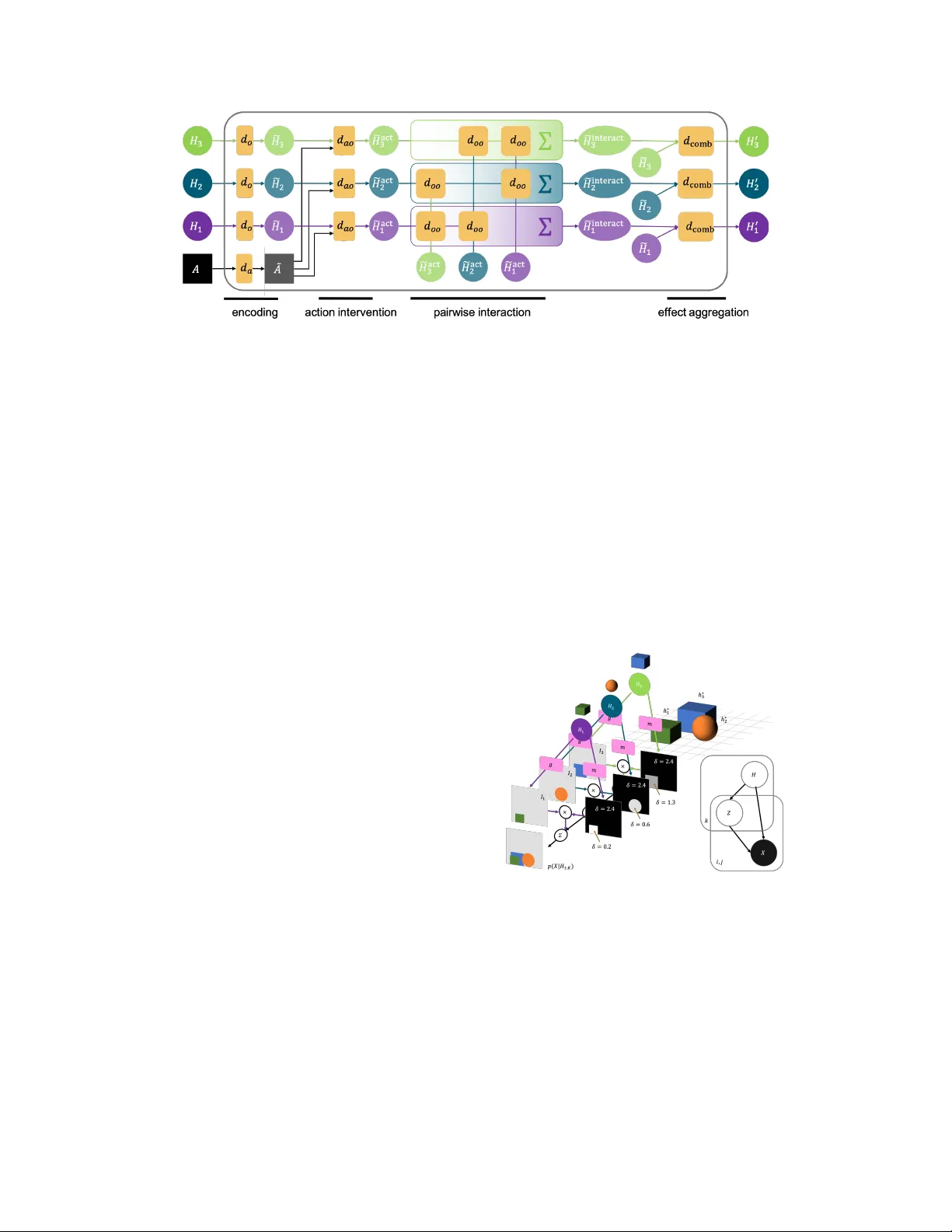
Entity Abstraction in V isual Model-Based Reinf orcement Lear ning Rishi V eerapaneni ∗ , 1 , John D . Co-Reyes ∗ , 1 , Michael Chang ∗ , 1 , Michael Janner 1 Chelsea Finn 2 , Jiajun W u 3 , Joshua B. T enenbaum 3 , Sergey Levine 1 Abstract: This paper tests the hypothesis that modeling a scene in terms of entities and their local interactions, as opposed to modeling the scene globally , provides a significant benefit in generalizing to physical tasks in a combinatorial space the learner has not encountered before. W e present object-centric perception, prediction, and planning (OP3), which to the best of our knowledge is the first fully probabilistic entity-centric dynamic latent variable framework for model- based reinforcement learning that acquires entity representations from raw visual observations without supervision and uses them to predict and plan. OP3 enforces entity-abstraction – symmetric processing of each entity representation with the same locally-scoped function – which enables it to scale to model different numbers and configurations of objects from those in training. Our approach to solving the ke y technical challenge of grounding these entity representations to actual objects in the en vironment is to frame this variable binding problem as an inference problem, and we de velop an interactive inference algorithm that uses temporal continuity and interacti ve feedback to bind information about object properties to the entity variables. On block-stacking tasks, OP3 generalizes to novel block configurations and more objects than observed during training, outperforming an oracle model that assumes access to object supervision and achie ving two to three times better accuracy than a state-of-the-art video prediction model that does not exhibit entity abstraction. Keyw ords: model-based reinforcement learning, objects, compositionality 1 Introduction A powerful tool for modeling the complexity of the physical world is to frame this complexity as the composition of simpler entities and processes. For example, the study of classical mechanics in terms of macroscopic objects and a small set of laws go verning their motion has enabled not only an explanation of natural phenomena like apples falling from trees but the inv ention of structures that nev er before existed in human history , such as skyscrapers. Paradoxically , the creativ e variation of such physical constructions in human society is due in part to the uniformity with which human models of physical laws apply to the literal b uilding blocks that comprise such structures – the reuse of the same simpler models that apply to primiti ve entities and their relations in different ways ob viates the need, and cost, of designing custom solutions from scratch for each construction instance. The challenge of scaling the generalization abilities of learning robots follows a similar characteristic to the challenges of modeling physical phenomena: the complexity of the task space may scale combinatorially with the configurations and number of objects, but if all scene instances share the same set of objects that follow the same physical laws, then transforming the problem of modeling scenes into a problem of modeling objects and the local physical processes that gov ern their interactions may provide a significant benefit in generalizing to solving novel physical tasks the learner has not encountered before. This is the central hypothesis of this paper . * Equal contribution. 1 Univ ersity of California Berkeley . 2 Stanford Univ ersity . 3 Massachusetts Institute of T echnology . Code and visualizations are av ailable at https://sites.google.com/view/op3website/ . This article is an extended v ersion of the manuscript published in CoRL 2019. 3rd Conference on Robot Learning (CoRL 2019), Osaka, Japan. Figure 1: OP3 . (a) OP3 can infer a set of entity variables H ( T ) 1: K from a series of interactions (interactiv e entity grounding) or a single image (entity grounding). OP3 rollouts predict the future entity states H ( T + d ) 1: K giv en a sequence of actions a ( T : T + d ) . W e ev aluate these rollouts during planning by scoring these predictions against inferred goal entity-states H ( G ) k . (b) OP3 enforces the entity abstraction , factorizing the latent state into local entity states, each of which are symmetrically processed with the same function that takes in a generic entity as an argument. In contrast, prior work either (c) process a global latent state [ 1 ] or (d) assume a fixed set of entities processed in a permutation-sensiti ve manner [ 2 – 5 ]. (e-g) Enforcing the entity-abstraction on modeling the (f) dynamics and (g) observation distrib utions of a POMDP , and on the (e) interactive infer ence procedure for grounding the entity variables in ra w visual observations. Actions are not shown to reduce clutter . W e test this hypothesis by defining models for percei ving and predicting ra w observations that are themselves compositions of simpler functions that operate locally on entities rather than globally on scenes. Importantly , the symmetry that all objects follo w the same physical laws enables us to define these learnable entity-centric functions to tak e as input argument a variable that represents a generic entity , the specific instantiations of which are all processed by the same function. W e use the term entity abstraction to refer to the abstraction barrier that isolates the abstract variable , which the entity-centric function is defined with respect to, from its concrete instantiation , which contains information about the appearance and dynamics of an object that modulates the function’ s behavior . Defining the observation and dynamic models of a model-based reinforcement learner as neural network functions of abstract entity variables allo ws for symbolic computation in the space of entities, but the key challenge for realizing this is to ground the v alues of these variables in the world from raw visual observ ations. Fortunately , the language of partially observable Markov decision processes (POMDP) enables us to represent these entity variables as latent random state v ariables in a state- factorized POMDP , thereby transforming the variable binding problem into an inference problem with which we can build upon state-of-the-art techniques in amortized iterative v ariational inference [ 6 – 8 ] to use temporal continuity and interactive feedback to infer the posterior distribution of the entity variables gi ven a sequence of observ ations and actions. W e present a framework for object-centric per ception, pr ediction, and planning (OP3), a model-based reinforcement learner that predicts and plans ov er entity v ariables inferred via an interactive infer ence algorithm from raw visual observ ations. Empirically OP3 learns to disco ver and bind information about actual objects in the en vironment to these entity variables without any supervision on what these variables should corr espond to. As all computation within the entity-centric function is local in scope with respect to its input entity , the process of modeling the dynamics or appearance of each object is pr otected from the computations in volv ed in modeling other objects, which allows OP3 to generalize to modeling a variable number of objects in a v ariety of contexts with no re-training. Contributions: Our conceptual contribution is the use of entity abstraction to integrate graphical models, symbolic computation, and neural networks in a model-based reinforcement learning (RL) agent. This is enabled by our technical contribution: defining models as the composition of locally- scoped entity-centric functions and the interacti ve inference algorithm for grounding the abstract entity v ariables in raw visual observ ations without any supervision on object identity . Empirically , we find that OP3 achie ves two to three times greater accuracy than state of the art video prediction models in solving nov el single and multi-step block stacking tasks. 2 Related W ork Representation learning for visual model-based reinf orcement learning: Prior works have pro- posed learning video prediction models [ 2 , 9 – 11 ] to improv e exploration [ 12 ] and planning [ 13 ] in RL. 2 Figure 2: Comparison with other methods. Unlike other methods, OP3 is a fully probabilistic factorized dynamic latent variable model, gi ving it se veral desirable properties. First, OP3 is naturally suited for combina- torial generalization [ 52 ] because it enforces that local properties are in variant to changes in global structure. Because ev ery learnable component of the OP3 operates symmetrically on each entity , including the mechanism that disambiguates entities itself (c.f. COBRA, which uses a learned autoregressi ve network to disambiguates entities, and T ransporter and C-SWMs, which use a forward pass of a con volutional encoder for the global scene, rather than each entity), the weights of OP3 are in variant to changes in the number of instances of an entity , as well as the number of entities in the scene. Second, OP3’ s recurrent structure makes it straightforward to enforce spatiotemporal consistency , object permanence, and refine the grounding of its entity representations ov er time with new information. In contrast, COBRA, T ransporter , and C-SWMs all model single-step dynamics and do not contain mechanisms for establishing a correspondence between the entity representations predicted from the previous timestep with the entity representations inferred at the current timestep. Ho wev er , such works and others that represent the scene with a single representation vector [ 1 , 14 – 16 ] may be susceptible to the binding problem [ 17 , 18 ] and must rely on data to learn that the same object in two dif ferent contexts can be modeled similarly . But processing a disentangled latent state with a single function [ 3 , 19 – 22 ] or processing each disentangled f actor in a permutation-sensiti ve manner [ 3 , 11 , 23 ] (1) assumes a fixed number of entities that cannot be dynamically adjusted for generalizing to more objects than in training and (2) has no constraints to enforce that multiple instances of the same entity in the scene be modeled in the same way . For generalization, often the particular arrangement of objects in a scene does not matter so much as what is constant across scenes – properties of indi vidual objects and inter-object relationships – which the inducti ve biases of these prior works do not capture. The entity abstraction in OP3 enforces symmetric processing of entity representations, thereby ov ercoming the limitations of these prior works. Unsupervised grounding of abstract entity v ariables in concrete objects: Prior w orks that model entities and their interactions often pre-specify the identity of the entities [ 24 – 30 ], provide additional supervision [ 31 – 34 ], or provide additional specification such as se gmentations [ 35 ], crops [ 36 ], or a simulator [ 37 , 38 ]. Those that do not assume such additional information often factorize the entire scene into pixel-lev el entities [ 39 – 41 ], which do not model objects as coherent wholes. None of these works solve the problem of grounding the entities in raw observation, which is crucial for autonomous learning and interaction. OP3 builds upon recently proposed ideas in grounding entity representations via inference on a symmetrically factorized generative model of static [ 8 , 17 , 42 ] and dynamic [ 43 ] scenes, whose advantage ov er other methods for grounding [ 5 , 44 – 47 ] is the ability to refine the grounding with new information. In contrast to other methods for binding in neural networks [ 48 – 51 ], formulating inference as a mechanism for variable binding allows us to model uncertainty in the values of the v ariables. Comparison with similar work: The closest three works to OP3 are the T ransporter [ 3 ], COBRA [ 5 ], and C-SWMs [ 53 ]. The Transporter enforces a sparsity bias to learn object keypoints, each represented as a feature vector at a pixel location, and the method’ s focus on keypoints has the adv antage of enabling long-term object tracking, modeling articulated composite bodies such as joints, and scaling to dozens of objects. C-SWMs learn entity representations using a contrastive loss, which has the advantage of overcoming the difficulty in attending to small but relev ant features as well as the 3 large model capacity requirements usually characteristic of the pixel reconstructi ve loss. COBRA uses the autoregressi ve attention-based MONet [ 46 ] architecture to obtain entity representations, which has the adv antage of being more computationally ef ficient and stable to train. Unlike works such as [ 8 , 42 , 45 , 46 ] that infer entity representations from static scenes, these works represent complementary approaches to OP3 (Figure 2 ) for representing dynamic scenes. Symmetric processing of entities – processing each entity representation with the same function, as OP3 does with its observation, dynamics, and refinement networks – enforces the in variance that local properties are in variant to changes in global structure because it prevents the processing of one entity from being af fected by other entities. How symmetric the process is for obtaining these entity representations from visual observation affects ho w straightforward it is to directly transfer models of a single entity across different global contexts, such as in modeling multiple instances of the same entity in the scene in a similar way or in generalizing to modeling different numbers of objects than in training. OP3 can exhibit this type of zero-shot transfer because the learnable components of its refinement process are fully symmetric across entities, which prev ents OP3 from ov erfitting to the global structure of the scene. In contrast, the Ke yNet encoder of the T ransporter and the CNN-encoder of C-SWMs associate the content of the entity representation with the index of that entity in a global representation vector (Figure 1 d), and this permutation-sensitive mapping entangles the encoding of an entity with the global structure of the scene. COBRA lies in between: it uses a learnable autoregressi ve attention network to infer se gmentation masks, which entangles local object segmentations with global structure b ut may provide a useful bias for attending to salient objects, and symmetrically encodes entity representations giv en these masks 5 . As a recurrent probabilistic dynamic latent variable model, OP3 can refine the grounding of its entity representations with new information from raw observations by simply applying a belief update similar to that used in filtering for hidden Marko v models. The T ransporter , COBRA, and C-SWMs all do not hav e mechanisms for updating the belief of the entity representations with information from subsequent image frames. W ithout recurrent structure, such methods rely on the assumption that a single forward pass of the encoder on a static image is sufficient to disambiguate objects, but this assumption is not generally true: objects can pop in and out of occlusion and what constitutes an object depends temporal cues, especially in real w orld settings. Recurrent structure is b uilt into the OP3 inference update (Appendix 2 ), enabling OP3 to model object permanence under occlusion and refine its object representations with new information in modeling real w orld videos (Figure 7 ). 3 Problem F ormulation Let x ∗ denote a physical scene and h ∗ 1: K denote the objects in the scene. Let X and A be random variables for the image observ ation of the scene x ∗ and the agent’ s actions respectiv ely . In contrast to prior works [ 1 ] that use a single latent v ariable to represent the state of the scene, we use a set of latent random variables H 1: K to represent the state of the objects h ∗ 1: K . W e use the term object to refer to h ∗ k , which is part of the physical world, and the term entity to refer to H k , which is part of our model of the physical w orld. The generati ve distrib ution of observations X (0: T ) and latent entities H (0: T ) 1: K from taking T actions a (0: T − 1) is modeled as: p  X (0: T ) , H (0: T ) 1: K    a (0: T − 1)  = p  H (0) 1: K  T Y t =1 p  H ( t ) 1: K    H ( t − 1) 1: K , a ( t − 1)  T Y t =0 p  X ( t )    H ( t ) 1: K  (1) where p ( X ( t ) | H ( t ) 1: K ) and p ( H ( t ) 1: K | H ( t − 1) 1: K , A ( t − 1) ) are the observation and dynamics distrib ution respecti vely shared across all timesteps t . Our goal is to build a model that, from simply observing raw observ ations of random interactions, can generalize to solve novel compositional object manipulation problems that the learner was ne ver trained to do, such as b uilding various block to wers during test time from only training to predict how blocks f all during training time. When all tasks follo w the same dynamics we can achie ve such generalization with a planning algo- rithm if giv en a sequence of actions we could compute p ( X ( T +1: T + d ) | X (0: T ) , A (0: T + d − 1) ) , the pos- terior predicti ve distrib ution of observ ations d steps into the future. Approximating this predictiv e dis- tribution can be cast as a variational inference problem (Appdx. B ) for learning the parameters of an ap- 5 A discussion of the adv antages and disadvantages of using an attention-based entity disambiguation method, which MONet and COBRA use, versus an iterativ e refinement method, which IODINE [ 8 ] and OP3 use, is discussed in Greff et al. [ 8 ]. 4 proximate observation distribution G ( X ( t ) | H ( t ) 1: K ) , dynamics distrib ution D ( H ( t ) 1: K | H ( t − 1) 1: K , A ( t − 1) ) , and a time-factorized recognition distribution Q ( H ( t ) 1: K | H ( t − 1) 1: K , X ( t ) , A ( t − 1) ) that maximize the evi- dence lower bound (ELBO), gi ven by L = P T t =0 L ( t ) r − L ( t ) c , where L t r = E h t 1: K ∼ q ( H t 1: K | h 0: t − 1 1: K ,x 1: t ,a 0: t − 1 )  log G  x t | h t 1: K  L t c = E h t − 1 1: K ∼ q ( H t − 1 1: K | h 1: t − 2 1: K ,x 1: t − 1 ,a 0: t − 2 )  D K L  Q  H t 1: K | h t − 1 1: K , x t , a t − 1  || D  H t 1: K | h t − 1 1: K , a t − 1  . The ELBO pushes Q to produce states of the entities H 1: K that contain information useful for not only reconstructing the observ ations via G in L ( t ) r but also for predicting the entities’ future states via D in L ( t ) c . Sec. 4 will next of fer our method for incorporating entity abstraction into modeling the generativ e distribution and optimizing the ELBO. 4 Object-Centric Per ception, Prediction, and Planning (OP3) The entity abstraction is deri ved from an assumption about symmetry: that the problem of modeling a dynamic scene of multiple entities can be reduced to the problem of (1) modeling a single entity and its interactions with an entity-centric function and (2) applying this function to e very entity in the scene. Our choice to represent a scene as a set of entities exposes an a venue for directly encoding such a prior about symmetry that would otherwise not be straightforw ard with a global state representation. As sho wn in Fig. 1 , a function F that respects the entity abstraction requires two ingredients. The first ingredient (Sec. 4.1 ) is that F ( H 1: K ) is expressed in part as the higher-order operation map ( f , H 1: K ) that broadcasts the same entity-centric function f ( H k ) to every entity variable H k . This yields the benefit of automatically transferring learned knowledge for modeling an individual entity to all entities in the scene rather than learn such symmetry from data. As f is a function that takes in a single generic entity variable H k as argument, the second ingredient (Sec. 4.2 ) should be a mechanism that binds information from the raw observ ation X about a particular object h ∗ k to the variable H k . 4.1 Entity Abstraction in the Observation and Dynamics Models The functions of interest in model-based RL are the observation and dynamics models G and D with which we seek to approximate the data-generating distribution in equation 1 . Observation Model: The observation model G ( X | H 1: K ) approximates the distribution p ( X | H 1: K ) , which models ho w the observ ation X is caused by the combination of entities H 1: K . W e enforce the entity abstraction in G (in Fig. 1 g) by applying the same entity-centric function g ( X | H k ) to each entity H k , which we can implement using a mixture model at each pixel ( i, j ) : G  X ( ij )   H 1: K  = K X k =1 m ( ij ) ( H k ) · g  X ( ij ) | H k  , (2) where g computes the mixture components that model ho w each individual entity H k is independently generated, combined via mixture weights m that model the entities’ relativ e depth from the camera, the deriv ation of which is in Appdx. A . Dynamics Model: The dynamics model D ( H 0 1: K | H 1: K , A ) approximates the distribution p ( H 0 1: K | H 1: K , A ) , which models how an action A intervenes on the entities H 1: K to produce their future v alues H 0 1: K . W e enforce the entity abstraction in D (in Fig. 1 f) by applying the same entity-centric function d ( H 0 k | H k , H [ 6 = k ] , A ) to each entity H k , which reduces the problem of mod- eling how an action affects a scene with a combinatorially large space of object configurations to the problem of simply modeling how an action af fects a single generic entity H k and its interactions with the list of other entities H [ 6 = k ] . Modeling the action as an finer-grained intervention on a single entity rather than the entire scene is a benefit of using local representations of entities rather than global representations of scenes. Howe ver , at this point we still ha ve to model the combinatorially large space of interactions that a single entity could participate in. Therefore, we can further enforce a pairwise entity abstraction on d by applying the same pairwise function d oo ( H k , H i ) to each entity pair ( H k , H i ) , for i ∈ [ 6 = k ] . 5 Figure 4: The dynamics model D models the time e volution of ev ery object by symmetrically applying the function d to each object. For a gi ven object, d models the individual dynamics of that object ( d o ) , embeds the action vector ( d a ) , computes the action’ s effect on that object ( d ao ) , computes each of the other objects’ effect on that object ( d oo ) , and aggregates these ef fects together ( d comb ) . Omitting the action to reduce clutter (the full form is written in Appdx. F .2 ), the structure of the D therefore follows this form: D  H 0 1: K   H 1: K  = K Y k =1 d  H 0 k    H k , H interact k  , where H interact k = K X i 6 = k d oo ( H i , H k ) . (3) The entity abstraction therefore provides the flexibility to scale to modeling a variable number of objects by solely learning a function d that operates on a single generic entity and a function d oo that operates on a single generic entity pair , both of which can be re-used for across all entity instances. 4.2 Interactive Infer ence f or Binding Object Properties to Latent V ariables Figure 3: (a) The observation model G models an observation image as a composition of sub-images weighted by segmentation masks. The shades of gray in the masks indicate the depth δ from the camera of the object that the sub-image depicts. (b) The graphical model of the generative model of observ ations, where k index es the entity , and i, j index es the pixel. Z is the indicator variable that signifies whether an object’ s depth at a pixel is the closest to the camera. For the observation and dynamics models to oper- ate from raw pixels hinges on the ability to bind the properties of specific physical objects h ∗ 1: K to the entity v ariables H 1: K . For latent v ariable models, we frame this v ariable binding problem as an inference problem: binding information about h ∗ 1: K to H 1: K can be cast as a problem of inferring the parameters of p ( H (0: T ) | x (0: T ) , a (0: T − 1) ) , the posterior distrib u- tion of H 1: K giv en a sequence of interactions. Maxi- mizing the ELBO in Sec. 3 offers a method for learn- ing the parameters of the observ ation and dynamics models while simultaneously learning an approxima- tion to the posterior q ( H (0: T ) | x (0: T ) , a (0: T − 1) ) = Q T t =0 Q ( H ( t ) 1: K | H ( t − 1) 1: K , x ( t ) , a ( t ) ) , which we have chosen to factorize into a per-timestep recognition dis- tribution Q shared across timesteps. W e also choose to enforce the entity abstraction on the process that computes the recognition distrib ution Q (in Fig. 1 e) by decomposing it into a recognition distribution q applied to each entity: Q  H ( t ) 1: K | h ( t − 1) 1: K , x ( t ) , a ( t )  = K Y k =1 q  H ( t ) k | h ( t − 1) k , x ( t ) , a ( t )  . (4) Whereas a neural network encoder is often used to approximate the posterior [ 1 , 3 , 4 ], a single forward pass that computes q in parallel for each entity is insufficient to break the symmetry for dividing responsibility of modeling dif ferent objects among the entity v ariables [ 54 ] because the entities do not hav e the opportunity to communicate about which part of the scene they are representing. 6 Figure 5: Amortized interactive infer ence alternates between refinement (pink) and dynamics (orange) steps, iterativ ely updating the belief of λ 1: K ov er time. ˆ λ corresponds to the output of the dynamics network, which serves as the initial estimate of λ that is subsequently refined by f G and f Q . O denotes the feedback used in the refinement process, which includes gradient information and auxiliary inputs (Appdx. D ). W e therefore adopt an iterative inference approach [ 6 ] to compute the recognition distribution Q , which has been shown to break symmetry among modeling objects in static scenes [ 8 ]. Iterative inference computes the recognition distribution via a procedur e , rather than a single forward pass of an encoder, that iteratively refines an initial guess for the posterior parameters λ 1: K by using gradients from how well the generati ve model is able to predict the observation based on the current posterior estimate. The initial guess provides the noise to break the symmetry . For scenes where position and color are enough for disambiguating objects, a static image may be suf ficient for inferring q . Howev er, in interacti ve en vironments disambiguating objects is more underconstrained because what constitutes an object depends on the goals of the agent. W e therefore incorporate actions into the amortized varitional filtering framework [ 7 ] to de velop an interactive infer ence algorithm (Appdx. D and Fig. 5 ) that uses temporal continuity and interactiv e feedback to disambiguate objects. Another benefit of enforcing entity abstraction is that preserving temporal consistency on entities comes for free: information about each object remains bound to its respective H k through time, mixing with information about other entities only through explicitly defined avenues, such as in the dynamics model. 4.3 T raining at Differ ent Timescales The variational parameters λ 1: K are the interface through which the neural networks f g , f d , f q that respecti vely output the distrib ution parameters of G , D , and Q communicate. For a particular dynamic scene, the execution of interactiv e inference optimizes the variational parameters λ 1: K . Acr oss scene instances, we train the weights of f g , f d , f q by backpropagating the ELBO through the entire inference procedure, spanning multiple timesteps. OP3 thus learns at three different timescales: the variational parameters learn (1) across M steps of inference within a single timestep and (2) across T timesteps within a scene instance, and the network weights learn (3) across different scene instances. Beyond next-step prediction, we can directly train to compute the posterior predicti ve distribu- tion p ( X ( T +1: T + d ) | x (0: T ) , a (0: T + d ) ) by sampling from the approximate posterior of H ( T ) 1: K with Q , rolling out the dynamics model D in latent space from these samples with a se quence of d actions, and predicting the observation X ( T + d ) with the observation model G . This approach to action- conditioned video prediction predicts future observations directly from observations and actions, b ut with a bottleneck of K time-persistent entity-v ariables with which the dynamics model D performs symbolic relational computation. 4.4 Object-Centric Planning OP3 rollouts, computed as the posterior predicti ve distribution, can be integrated into the standard visual model-predictive control [ 13 ] framework. Since interactiv e inference grounds the entities H 1: K in the actual objects h ∗ 1: K depicted in the ra w observ ation, this grounding essentially gi ves OP3 access to a pointer to each object, enabling the rollouts to be in the space of entities and their relations. 7 These pointers enable OP3 to not merely predict in the space of entities, but give OP3 access to an object-centric action space : for example, instead of being restricted to the standard (pick xy, place xy) action space common to many manipulation tasks, which often requires biased picking with a scripted policy [ 55 , 56 ], these pointers enable us to compute a mapping (Appdx. G.2 ) between entity id and pick xy , allowing OP3 to automatically use a (entity id, place xy) action space without needing a scripted policy . 4.5 Generalization to V arious T asks W e consider tasks defined in the same environment with the same physical laws that gov ern appearance and dynamics. T asks are differentiated by goals, in particular goal configurations of objects. Building good cost functions for real world tasks is generally difficult [ 57 ] because the underlying state of the environment is always unobserved and can only be modeled through modeling observations. Ho wev er , by representing the en vironment state as the state of its entities, we may obtain finer-grained goal-specification without the need for manual annotations [ 58 ]. Having rolled out OP3 to a particular timestep, we construct a cost function to compare the predicted entity states H ( P ) 1: K with the entity states H ( G ) 1: K inferred from a goal image by considering pairwise distances between the entities, another example of enforcing the pairwise entity abstraction. Letting S 0 and S denote the set of goal and predicted entities respecti vely , we define the form of the cost function via a composition of the task specific distance function c operating on entity-pairs: C  H ( G ) 1: K , H ( P ) 1: K  = X a ∈ S 0 min b ∈ S c  H ( G ) a , H ( P ) b  , (5) in which we pair each goal entity with the closest predicted entity and sum ov er the costs of these pairs. Assuming a single action suf fices to mo ve an object to its desired goal position, we can greedily plan each timestep by defining the cost to be min a ∈ S 0 ,b ∈ S c ( H ( G ) a , H ( P ) b ) , the pair with minimum distance, and removing the corresponding goal entity from further consideration for future planning. 5 Experiments Our experiments aim to study to what de gree entity abstraction impro ves generalization, planning, and modeling. Sec. 5.1 shows that from only training to predict ho w objects fall, OP3 generalizes to solve v arious novel block stacking tasks with tw o to three times better accurac y than a state-of-the-art video prediction model. Sec. 5.2 shows that OP3 can plan for multiple steps in a dif ficult multi-object en vironment. Sec. 5.3 shows that OP3 learns to ground its abstract entities in objects from real world videos. 5.1 Combinatorial Generalization without Object Supervision W e first inv estigate how well OP3 can learn object-based representations without additional ob- ject supervision, as well as how well OP3’ s factorized representation can enable combinatorial generalization for scenes with many objects. Domain: In the MuJoCo [ 59 ] block stacking task introduced by Janner et al. [ 35 ] for the O2P2 model, a block is raised in the air and the model must predict the steady-state effects of dropping the block on a surface with multiple objects, which implicitly requires modeling the effects of gravity and collisions. The agent is nev er trained to stack blocks, b ut is tested on a suite of tasks where it must construct block to wer specified by a goal image. Janner et al. [ 35 ] showe d that an object-centric model with access to gr ound truth object segmentations can solve these tasks with about 76% accuracy . W e now consider whether OP3 can do better , but without any supervision on object identity . SA VP O2P2 OP3 (ours) 24% 76% 82% T able 1: Accuracy (%) of block to wer builds by the SA VP baseline, the O2P2 oracle, and our approach. O2P2 uses image segmenta- tions whereas OP3 uses only raw images as input. # Blocks SA VP OP3 (xy) OP3 (entity) 1 54% 73% 91% 2 28% 55% 80% 3 28% 41% 55% T able 2: Accuracy (%) of multi-step planning for building block towers. (xy) means (pick xy, place xy) action space while (entity) means (entity id, place xy) action space. 8 Setup: W e train OP3 on the same dataset and ev aluate on the same goal images as Janner et al. [ 35 ] . While the training set contains up to fiv e objects, the test set contains up to nine objects, which are placed in specific structures (bridge, pyramid, etc.) not seen during training. The actions are optimized using the cross-entropy method (CEM) [ 60 ], with each sampled action e valuated by the greedy cost function described in Sec. 4.5 . Accuracy is ev aluated using the metric defined by Janner et al. [ 35 ], which checks that all blocks are within some threshold error of the goal. Results: The two baselines, SA VP [ 11 ] and O2P2, represent the state-of-the-art in video prediction and symmetric object-centric planning methods, respectively . SA VP models objects with a fixed number of conv olutional filters and does not process entities symmetrically . O2P2 does process entities symmetrically , but requires access to ground truth object se gmentations. As shown in T able 1 , OP3 achiev es better accurac y than O2P2, e ven without an y ground truth supervision on object identity , possibly because grounding the entities in the ra w image may provide a richer conte xtual representation than encoding each entity separately without such global context as O2P2 does. OP3 achiev es three times the accuracy of SA VP , which suggests that symmetric modeling of entities is enables the flexibility to transfer knowledge of dynamics of a single object to novel scenes with different configurations heights, color combinations, and numbers of objects than those from the training distribution. Fig. 8 and Fig. 9 in the Appendix show that, by grounding its entities in objects of the scene through inference, OP3’ s predictions isolates only one object at a time without affecting the predictions of other objects. Figure 6: (a) In the block stacking task from [ 35 ] with single-step greedy planning, OP3’ s generalizes better than both O2P2, an oracle model with access to image segmentations, and SA VP , which does not enforce entity abstraction. (b) OP3 exhibits better multi-step planning with objects already present in the scene. By planning with MPC using random pick locations (SA VP and OP3 (xy)), the sparsity of objects in the scene mak e it rare for random pick locations to actually pick the objects. Howe ver , because OP3 has access to pointers to the latent entities, we can use these to automatically bias the pick locations to be at the object location, without any supervision (OP3 (entity)). 5.2 Multi-Step Planning The goal of our second experiment is to understand ho w well OP3 can perform multi-step planning by manipulating objects already present in the scene. W e modify the block stacking task by changing the action space to represent a picking and dropping location. This requires reasoning over e xtended action sequences since moving objects out of place may be necessary . Goals are specified with a goal image, and the initial scene contains all of the blocks needed to build the desired structure. This task is more dif ficult because the agent may ha ve to mov e blocks out of the way before placing other ones which would require multi-step planning. Furthermore, an action only successfully picks up a block if it intersects with the block’ s outline, which makes searching through the combinatorial space of plans a challenge. As stated in Sec. 4.4 , having a pointer to each object enables OP3 to plan in the space of entities. W e compare two different action spaces (pick xy, place xy) and (entity id, place xy) to understand how automatically filtering 9 for pick locations at actual locations of objects enables better efficiency and performance in planning. Details for determining the pick xy from entity id are in appendix G.2 . Results: W e compare with SA VP , which uses the (pick xy, place xy) action space. With this standard action space (T able 2 ) OP3 achieves between 1.5-2 times the accuracy of SA VP . This performance gap increases to 2-3 times the accurac y when OP3 uses the (entity id, place xy) action space. The low performance of SA VP with only tw o blocks highlights the dif ficulty of such combinatorial tasks for model-based RL methods, and highlights the both the generalization and localization benefits of a model with entity abstraction. Fig. 6 b sho ws that OP3 is able to plan more ef ficiently , suggesting that OP3 may be a more ef fectiv e model than SA VP in modeling combinatorial scenes. Fig. 7 a shows the e xecution of interacti ve inference during training, where OP3 alternates between four refinement steps and one prediction step. Notice that OP3 infers entity representations that decompose the scene into coherent objects and that entities that do not model objects model the background. W e also observ e in the last column ( t = 2 ) that OP3 predicts the appearance of the green block ev en though the green block was partially occluded in the previous timestep, which sho ws its ability to retain information across time. Figure 7: V isualization of interactiv e inference for block-manipulation and real-world videos [ 61 ]. Here, OP3 interacts with the objects by executing pre-specified actions in order to disambiguate objects already present in the scene by taking adv antage of temporal continuity and recei ving feedback from how well its prediction of how an action af fects an object compares with the ground truth result. (a) OP3 does four refinement steps on the first image, and then 2 refinement steps after each prediction. (b) W e compare OP3, applied on dynamic videos, with IODINE, applied independently to each frame of the video, to illustrate that using a dynamics model to propagate information across time enables better object disambiguation. W e observe that initially , both OP3 (green circle) and IODINE (cyan circles) both disambiguate objects via color segmentation because color is the only signal in a static image to group pixels. Howe ver , we observe that as time progresses, OP3 separates the arm, object, and background into separate latents (purple) by using its currently estimates latents predict the ne xt observation and comparing this prediction with the actually observ ed next observ ation. In contrast, applying IODINE on a per-frame basis does not yield benefits of temporal consistenc y and interactiv e feedback (red). 5.3 Real W orld Evaluation The pre vious tasks used simulated en vironments with monochromatic objects. Now we study ho w well OP3 scales to real world data with cluttered scenes, object ambiguity , and occlusions. W e ev aluate OP3 on the dataset from Ebert et al. [ 61 ] which contains videos of a robotic arm moving cloths and other deformable and multipart objects with varying te xtures. W e ev aluate qualitativ e performance by visualizing the object se gmentations and compare against vanilla IODINE, which does not incorporate an interaction-based dynamics model into the inference process. Fig. 7 b highlights the strength of OP3 in preserving temporal continuity and disambiguating objects in real world scenes. While IODINE can disambiguate monochromatic objects in static images, we observe that it struggles to do more than just color se gmentation on more complicated images where movement is required to disambiguate objects. In contrast, OP3 is able to use temporal information to obtain more accurate segmentations, as seen in Fig. 7 b where it initially performs color segmentation by grouping the to wel, arm, and dark container edges together, and then by observing the effects of mo ving the arm, separates these entities into different groups. 10 6 Discussion W e have sho wn that enforcing the entity abstraction in a model-based reinforcement learner improves generalization, planning, and modeling across various compositional multi-object tasks. In particular, enforcing the entity abstraction provides the learner with a pointer to each entity v ariable, enabling us to define functions that are local in scope with respect to a particular entity , allowing kno wledge about an entity in one context to directly transfer to modeling the same entity in different contexts. In the physical world, entities are often manifested as objects, and generalization in physical tasks such as robotic manipulation often may require symbolic reasoning about objects and their interactions. Howe ver , the general difficulty with using purely symbolic, abstract representations is that it is unclear how to continuously update these representations with more raw data. OP3 frames such symbolic entities as random v ariables in a dynamic latent v ariable model and infers and refines the posterior of these entities over time with neural networks. This suggests a potential bridge to connect abstract symbolic variables with the noisy , continuous, high-dimensional physical world, opening a path to scaling robotic learning to more combinatorially complex tasks. Acknowledgments The authors would like to thank the anon ymous re viewers for their helpful feedback and comments. The authors would also like to thank Sjoerd van Steenkiste, Nalini Singh and Marvin Zhang for helpful discussions on the graphical model, Klaus Greff for help in implementing IODINE, Alex Lee for help in running SA VP , T om Griffiths, Karl Persch, and Oleg Rybkin for feedback on earlier drafts, Joe Marino for discussions on iterati ve inference, and Sam T oyer , Anirudh Goyal, Jessica Hamrick, Peter Battaglia, Loic Matthey , Y ash Sharma, and Gary Marcus for insightful discussions. This research was supported in part by the National Science Foundation under IIS-1651843, IIS-1700697, and IIS-1700696, the Of fice of Na val Research, ARL DCIST CRA W911NF-17-2-0181, D ARP A, Berkeley DeepDri ve, Google, Amazon, and NVIDIA. 11 References [1] D. Hafner, T . Lillicrap, I. Fischer, R. V illegas, D. Ha, H. Lee, and J. Davidson. Learning latent dynamics for planning from pixels. arXiv:1811.04551 , 2018. [2] C. Finn, I. Goodfellow , and S. Levine. Unsupervised learning for physical interaction through video prediction. In Advances in neural information pr ocessing systems , pages 64–72, 2016. [3] T . Kulkarni, A. Gupta, C. Ionescu, S. Borgeaud, M. Reynolds, A. Zisserman, and V . Mnih. Unsupervised learning of object keypoints for perception and control. , 2019. [4] Z. Xu, Z. Liu, C. Sun, K. Murphy , W . T . Freeman, J. B. T enenbaum, and J. W u. Modeling parts, structure, and system dynamics via predictiv e learning. 2018. [5] N. W atters, L. Matthey , M. Bosnjak, C. P . Burgess, and A. Lerchner. Cobra: Data-efficient model-based rl through unsupervised object discovery and curiosity-dri ven exploration. , 2019. [6] J. Marino, Y . Y ue, and S. Mandt. Iterative amortized inference. , 2018. [7] J. Marino, M. Cvitk ovic, and Y . Y ue. A general method for amortizing variational filtering. In Advances in Neural Information Pr ocessing Systems , pages 7857–7868, 2018. [8] K. Greff, R. L. Kaufmann, R. Kabra, N. W atters, C. Burgess, D. Zoran, L. Matthey , M. Botvinick, and A. Lerchner . Multi-object representation learning with iterativ e variational inference. , 2019. [9] N. Wichers, R. V illegas, D. Erhan, and H. Lee. Hierarchical long-term video prediction without supervision. , 2018. [10] E. L. Denton et al. Unsupervised learning of disentangled representations from video. In Advances in neural information processing systems , pages 4414–4423, 2017. [11] A. X. Lee, R. Zhang, F . Ebert, P . Abbeel, C. Finn, and S. Le vine. Stochastic adversarial video prediction. , 2018. [12] J. Oh, X. Guo, H. Lee, R. L. Lewis, and S. Singh. Action-conditional video prediction using deep networks in atari games. In Advances in neural information pr ocessing systems , pages 2863–2871, 2015. [13] C. Finn and S. Levine. Deep visual foresight for planning robot motion. In Robotics and Automation (ICRA), 2017 IEEE International Confer ence on , pages 2786–2793. IEEE, 2017. [14] M. Zhang, S. V ikram, L. Smith, P . Abbeel, M. J. Johnson, and S. Levine. Solar: Deep structured latent representations for model-based reinforcement learning. , 2018. [15] V . Mnih, K. Kavukcuoglu, D. Silver, A. A. Rusu, J. V eness, M. G. Bellemare, A. Graves, M. Riedmiller, A. K. Fidjeland, G. Ostrovski, S. Petersen, C. Beattie, A. Sadik, I. Antonoglou, H. King, D. Kumaran, D. Wierstra, S. Legg, and D. Hassabis. Human-lev el control through deep reinforcement learning. Natur e , 518(7540):529–533, 02 2015. [16] J. Oh, V . Chockalingam, S. Singh, and H. Lee. Control of memory, acti ve perception, and action in minecraft. , 2016. [17] K. Greff, R. K. Sriv astava, and J. Schmidhuber . Binding via reconstruction clustering. , 2015. [18] F . Rosenblatt. Principles of neurodynamics. perceptrons and the theory of brain mechanisms. T echnical report, CORNELL AER ONA U- TICAL LAB INC BUFF ALO NY , 1961. [19] W . F . Whitney , M. Chang, T . Kulkarni, and J. B. T enenbaum. Understanding visual concepts with continuation learning. arXiv:1602.06822 , 2016. [20] X. Chen, Y . Duan, R. Houthooft, J. Schulman, I. Sutske ver , and P . Abbeel. Infogan: Interpretable representation learning by information maximizing generativ e adversarial nets. In Advances in Neural Information Pr ocessing Systems , pages 2172–2180, 2016. [21] T . D. Kulkarni, W . F . Whitney , P . Kohli, and J. T enenbaum. Deep con volutional inverse graphics network. In Advances in Neural Information Pr ocessing Systems , pages 2539–2547, 2015. [22] V . Goel, J. W eng, and P . Poupart. Unsupervised video object segmentation for deep reinforcement learning. , 2018. [23] Z. Xu, Z. Liu, C. Sun, K. Murphy , W . T . Freeman, J. B. T enenbaum, and J. W u. Unsupervised disco very of parts, structure, and dynamics. arXiv:1903.05136 , 2019. [24] M. B. Chang, T . Ullman, A. T orralba, and J. B. T enenbaum. A compositional object-based approach to learning physical dynamics. arXiv:1612.00341 , 2016. [25] P . Battaglia, R. P ascanu, M. Lai, D. J. Rezende, et al. Interaction networks for learning about objects, relations and physics. In Advances in Neural Information Pr ocessing Systems , pages 4502–4510, 2016. [26] J. B. Hamrick, A. J. Ballard, R. Pascanu, O. V inyals, N. Heess, and P . W . Battaglia. Metacontrol for adaptiv e imagination-based optimization. , 2017. [27] M. Janner, K. Narasimhan, and R. Barzilay . Representation learning for grounded spatial reasoning. T ransactions of the Association for Computational Linguistics , 6:49–61, 2018. [28] K. Narasimhan, R. Barzilay , and T . Jaakkola. Grounding language for transfer in deep reinforcement learning. Journal of Artificial Intelligence Resear ch , 63:849–874, 2018. [29] V . Bapst, A. Sanchez-Gonzalez, C. Doersch, K. L. Stachenfeld, P . K ohli, P . W . Battaglia, and J. B. Hamrick. Structured agents for physical construction. , 2010. [30] A. Ajay , M. Bauza, J. W u, N. Fazeli, J. B. T enenbaum, A. Rodriguez, and L. P . Kaelbling. Combining physical simulators and object- based networks for control. , 2019. [31] R. Girshick, J. Donahue, T . Darrell, and J. Malik. Rich feature hierarchies for accurate object detection and semantic segmentation. In Pr oceedings of the IEEE conference on computer vision and pattern r ecognition , pages 580–587, 2014. [32] K. He, G. Gkioxari, P . Doll ´ ar , and R. Girshick. Mask r-cnn. In Pr oceedings of the IEEE international conference on computer vision , pages 2961–2969, 2017. [33] D. W ang, C. Devin, Q.-Z. Cai, F . Y u, and T . Darrell. Deep object centric policies for autonomous driving. , 2018. [34] W . Y ang, X. W ang, A. Farhadi, A. Gupta, and R. Mottaghi. Visual semantic na vigation using scene priors. , 2018. [35] M. Janner, S. Levine, W . T . Freeman, J. B. T enenbaum, C. Finn, and J. Wu. Reasoning about physical interactions with object-oriented prediction and planning. , 2018. [36] K. Fragkiadaki, P . Agrawal, S. Levine, and J. Malik. Learning visual predictive models of ph ysics for playing billiards. , 2015. [37] J. W u, E. Lu, P . Kohli, B. Freeman, and J. T enenbaum. Learning to see physics via visual de-animation. In Advances in Neural Information Pr ocessing Systems , pages 153–164, 2017. [38] K. Kansky , T . Silver , D. A. M ´ ely , M. Eldawy , M. L ´ azaro-Gredilla, X. Lou, N. Dorfman, S. Sidor, S. Phoenix, and D. George. Schema networks: Zero-shot transfer with a generative causal model of intuiti ve physics. , 2017. 12 [39] A. Santoro, D. Raposo, D. G. Barrett, M. Malinowski, R. Pascanu, P . Battaglia, and T . Lillicrap. A simple neural network module for relational reasoning. , 2017. [40] V . Zambaldi, D. Raposo, A. Santoro, V . Bapst, Y . Li, I. Babuschkin, K. Tuyls, D. Reichert, T . Lillicrap, E. Lockhart, et al. Deep reinforcement learning with relational inductiv e biases. 2018. [41] Y . Du and K. Narasimhan. T ask-agnostic dynamics priors for deep reinforcement learning. , 2019. [42] K. Greff, S. van Steenkiste, and J. Schmidhuber . Neural expectation maximization. 2017. [43] S. van Steenkiste, M. Chang, K. Greff, and J. Schmidhuber . Relational neural expectation maximization: Unsupervised discovery of objects and their interactions. , 2018. [44] G. Zhu, J. W ang, Z. Ren, and C. Zhang. Object-oriented dynamics learning through multi-lev el abstraction. , 2019. [45] S. A. Eslami, N. Heess, T . W eber, Y . T assa, D. Szepesvari, G. E. Hinton, et al. Attend, infer, repeat: Fast scene understanding with generativ e models. In Advances in Neural Information Pr ocessing Systems , pages 3225–3233, 2016. [46] C. P . Burgess, L. Matthey , N. W atters, R. Kabra, I. Higgins, M. Botvinick, and A. Lerchner . Monet: Unsupervised scene decomposition and representation. , 2019. [47] A. R. Kosiorek, H. Kim, I. Posner, and Y . W . Teh. Sequential attend, infer , repeat: Generativ e modelling of moving objects. arXiv:1806.01794 , 2018. [48] S. D. Levy and R. Gayler . V ector symbolic architectures: A new building material for artificial general intelligence. In Confer ence on Artificial General Intelligence , 2008. [49] P . Kanerva. Hyperdimensional computing: An introduction to computing in distributed representation with high-dimensional random vectors. Cognitive computation , 2009. [50] P . Smolensky . T ensor product variable binding and the representation of symbolic structures in connectionist systems. Artificial intelli- gence , 46(1-2):159–216, 1990. [51] A. V aswani, N. Shazeer, N. Parmar, J. Uszkoreit, L. Jones, A. N. Gomez, Ł. Kaiser, and I. Polosukhin. Attention is all you need. In Advances in neural information pr ocessing systems , pages 5998–6008, 2017. [52] P . W . Battaglia, J. B. Hamrick, V . Bapst, A. Sanchez-Gonzalez, V . Zambaldi, M. Malinowski, A. T acchetti, D. Raposo, A. Santoro, R. Faulkner , et al. Relational inductiv e biases, deep learning, and graph networks. , 2018. [53] T . Kipf, E. van der Pol, and M. W elling. Contrastiv e learning of structured world models. arXiv pr eprint arXiv:1911.12247 , 2019. [54] Y . Zhang, J. Hare, and P .-B. Adam. Deep set prediction networks. , 2019. [55] S. Levine, P . Pastor , A. Krizhevsk y , J. Ibarz, and D. Quillen. Learning hand-eye coordination for robotic grasping with deep learning and large-scale data collection. The International Journal of Robotics Resear ch , 37(4-5):421–436, 2018. [56] D. Kalashnikov , A. Irpan, P . Pastor , J. Ibarz, A. Herzog, E. Jang, D. Quillen, E. Holly , M. Kalakrishnan, V . V anhoucke, et al. Qt-opt: Scalable deep reinforcement learning for vision-based robotic manipulation. arXiv pr eprint arXiv:1806.10293 , 2018. [57] J. Fu, A. Singh, D. Ghosh, L. Y ang, and S. Levine. V ariational in verse control with events: A general framework for data-driven re ward definition. In Advances in Neural Information Pr ocessing Systems , pages 8538–8547, 2018. [58] F . Ebert, C. Finn, S. Dasari, A. Xie, A. Lee, and S. Levine. Visual foresight: Model-based deep reinforcement learning for vision-based robotic control. , 2018. [59] E. T odorov , T . Erez, and Y . T assa. Mujoco: A physics engine for model-based control. In 2012 IEEE/RSJ International Conference on Intelligent Robots and Systems , pages 5026–5033. IEEE, 2012. [60] R. Y . Rubinstein and D. P . Kroese. The cross-entropy method. In Information Science and Statistics , 2004. [61] F . Ebert, S. Dasari, A. X. Lee, S. Levine, and C. Finn. Robustness via retrying: Closed-loop robotic manipulation with self-supervised learning. , 2018. [62] C. Doersch. Tutorial on v ariational autoencoders. arXiv preprint , 2016. [63] D. P . Kingma and M. W elling. Auto-encoding variational bayes. , 2013. [64] D. J. Rezende, S. Mohamed, and D. Wierstra. Stochastic backpropagation and approximate inference in deep generative models. arXiv pr eprint arXiv:1401.4082 , 2014. [65] R. J. Williams and D. Zipser. A learning algorithm for continually running fully recurrent neural networks. Neural computation , 1(2): 270–280, 1989. [66] D. P . Kingma and J. Ba. Adam: A method for stochastic optimization. , 2014. [67] R. Pascanu, T . Mikolov , and Y . Bengio. Understanding the exploding gradient problem. ArXiv , abs/1211.5063, 2012. 13 A Observation Model The observ ation model G models ho w the objects H 1: K cause the image observ ation X ∈ R N × M . Here we provide a mechanistic justification for our choice of observ ation model by formulating the observation model as a probabilistic approximation to a deterministic rendering engine. Deterministic rendering engine: Each object H k is rendered independently as the sub-image I k and the resulting K sub-images are combined to form the final image observ ation X . T o combine the sub-images, each pixel I k ( ij ) in each sub-image is assigned a depth δ k ( ij ) that specifies the distance of object k from the camera at coordinate ( ij ) . of the image plane. Thus the pixel X ( ij ) takes on the v alue of its corresponding pixel I k ( ij ) in the sub-image I k if object k is closest to the camera than the other objects, such that X ( ij ) = K X k =1 Z k ( ij ) · I k ( ij ) , (6) where Z k ( ij ) is the indicator random variable 1 [ k = argmin k ∈ K δ k ( ij ) ] , allowing us to intuitiv ely interpret Z k as segmentation masks and I k as color maps. Modeling uncertainty with the obser vation model: In reality we do not directly observe the depth values, so we must construct a probabilistic model to model our uncertainty: G ( X | H 1: K ) = N ,M Y i,j =1 K X k =1 m ( ij ) ( H k ) · g  X ( ij ) | H k  , (7) where ev ery pixel ( ij ) is modeled through a set of mixture components g  X ( ij ) | H k  := p  X ij | Z k ( ij ) = 1 , H k  that model how pix els of the individual sub-images I k are generated, as well as through the mixture weights m ij ( H k ) := p  Z k ( ij ) = 1 | H k  that model which point of each object is closest to the camera. B Evidence Lower Bound Here we provide a deri vation of the e vidence lo wer bound. W e begin with the log probability of the observations X (1: T ) conditioned on a sequence of actions a (0: T − 1) : log p  X (0: T )    a (0: T − 1)  = log Z h (0: T ) 1: K p  X (0: T ) , h (0: T ) 1: K    a (0: T − 1)  dh (0: T ) 1: K . = log Z h (0: T ) 1: K p  X (0: T ) , h (0: T ) 1: K    a (0: T − 1)  q  h (0: T ) 1: K    ·  q  h (0: T ) 1: K    ·  dh (0: T ) 1: K . = log E h (0: T ) 1: K ∼ q  H (0: T ) 1: K    ·    p  X (0: T ) , h (0: T ) 1: K    a (0: T − 1)  q  h (0: T ) 1: K    ·    ≥ E h (0: T ) 1: K ∼ q  H (0: T ) 1: K    ·  log   p  X (0: T ) , h (0: T ) 1: K    a (0: T − 1)  q  h (0: T ) 1: K    ·    . (8) W e have freedom to choose the approximating distribution q  H (0: T ) 1: K    ·  so we choose it to be conditioned on the past states and actions, factorized across time: q  H (0: T ) 1: K    x (0: T ) , a (0: T )  = q  H (0) 1: K | x (0)  T Y t =1 q  H ( t ) 1: K    H ( t − 1) 1: K , x ( t ) , a ( t − 1)  W ith this factorization, we can use linearity of expectation to decouple Equation 8 across timesteps: E h (0: T ) 1: K ∼ q  H (0: T ) 1: K | x (0: T ) ,a (0: T )  log   p  X (0: T ) , h (0: T ) 1: K    a (0: T − 1)  q  h (0: T ) 1: K | x (0: T ) , a (0: T )    = ( t ) X t =0 L ( t ) r − L ( t ) c , 14 where at the first timestep L (0) r = E h (0) 1: K ∼ q  H (0) 1: K    X (0)  h log p  X (0)    h (0) 1: K i L (0) c = D K L  q  H (0) 1: K    X (0)  || p  H (0) 1: K  and at subsequent timesteps L ( t ) r = E h ( t ) 1: K ∼ q  H ( t ) 1: K | h (0: t − 1) 1: K ,X (0: t ) ,a (0: t − 1)  h log p  X ( t )    h ( t ) 1: K i L ( t ) c = E h ( t − 1) 1: K ∼ q  H ( t − 1) 1: K | h (0: t − 2) 1: K ,X (1: t − 1) ,a (0: t − 2)  h D K L  q  H ( t ) 1: K    h ( t − 1) 1: K , X ( t ) , a ( t − 1)  || p  H ( t ) 1: K    h ( t − 1) 1: K , a ( t − 1) i . By the Markov property , the marginal q ( H ( t ) 1: K | h (0: t − 1) 1: K , X (0: t ) , a (0: t − 1) ) is computed recursiv ely as E h ( t − 1) ∼ q  H ( t − 1) 1: K | h (0: t − 2) 1: K ,X (0: t − 1) ,a (0: t − 2)  h q  H ( t ) 1: K    h ( t − 1) 1: K , X ( t ) , a ( t − 1) i whose base case is q  H (0) | X (0)  when t = 0 . W e approximate observ ation distribution p ( X | H 1: K ) and the dynamics distribution p ( H 0 1: K | H 1: K , a ) by learning the parameters of the observation model G and dynamics model D respectiv ely as outputs of neural networks. W e approximate the recognition distribution q ( H ( t ) 1: K | h ( t − 1) 1: K , X ( t ) , a ( t − 1) ) via an inference procedure that refines better estimates of the posterior parameters, computed as an output of a neural network. T o compute the expectation in the marginal q ( H ( t ) 1: K | h (0: t − 1) 1: K , X (0: t ) , a (0: t − 1) ) , we follow standard practice in amortized variational inference by approximating the expectation with a single sample of the sequence h (0: t − 1) 1: K by sequentially sampling the latents for one timestep gi ven latents from the pre vious timestep, and optimizing the ELBO via stochastic gradient ascent [ 62 – 64 ]. C Posterior Pr edictive Distrib ution Here we provide a deriv ation of the posterior predictiv e distribution for the dynamic latent vari- able model with multiple latent states. Section B described ho w we compute the distributions p ( X | H 1: K ) , p ( H 0 1: K | H 1: K , a ) , q ( H ( t ) 1: K | h ( t − 1) 1: K , X ( t ) , a ( t − 1) ) , and q ( H (0: T ) 1: K | x (1: T ) , a (1: T ) ) . Here we show that these distributions can be used to approximate the predictiv e posterior distribution p ( X ( T +1: T + d ) | x (0: T ) , a (0: T + d ) ) by maximizing the follo wing lower bound: log p  X ( T +1: T + d )    x (0: T ) , a (0: T + d )  = Z h (0: T + d ) 1: K p  X ( T +1: T + d ) , h (0: T + d ) 1: K    x (0: T ) , a (0: T + d )  dh (0: T + d ) 1: K = Z h (0: T + d ) 1: K p  X ( T +1: T + d ) , h (0: T + d ) 1: K    x (0: T ) , a (0: T + d )  q  h (0: T + d ) 1: K    ·  q  h (0: T + d ) 1: K    ·  dh (0: T + d ) 1: K = log E h (0: T + d ) 1: K ∼ q  H (0: T + d ) 1: K    ·    p  X ( T +1: T + d ) , h (0: T + d ) 1: K    x (0: T ) , a (0: T + d )  q  h (0: T + d ) 1: K    ·    ≥ E h (0: T + d ) 1: K ∼ q  H (0: T + d ) 1: K    ·  log   p  X ( T +1: T + d ) , h (0: T + d ) 1: K    x (0: T ) , a (0: T + d )  q  h (0: T + d ) 1: K    ·    . (9) The numerator p ( X ( T +1: T + d ) , h (0: T + d ) 1: K | x (0: T ) , a (0: T + d ) ) can be decomposed into tw o terms, one of which in volving the posterior p ( h (0: T + d ) 1: K | x (0: T ) , a (0: T + d ) ) : p  X ( T +1: T + d ) , h (0: T + d ) 1: K    x (0: T ) , a (0: T + d )  = p  X ( T +1: T + d )    h (0: T + d ) 1: K  p  h (0: T + d ) 1: K    x (0: T ) , a (0: T + d )  , This allows Equation 9 to be brok en up into two terms: E h (0: T + d ) 1: K ∼ q  H (0: T + d ) 1: K    ·  log p  X ( T +1: T + d )    h (0: T + d ) 1: K  − D K L  q  H (0: T + d ) 1: K    ·  || p  H (0: T + d ) 1: K    x (0: T ) , a (0: T + d )  15 Maximizing the second term, the negativ e KL-diver gence between the variational distribution q ( H (0: T + d ) 1: K | · ) and the posterior p ( H (0: T + d ) 1: K | x (0: T ) , a (0: T + d ) ) is the same as maximizing the fol- lowing lo wer bound: E h (0: T ) 1: K ∼ q  h (0: T ) 1: K    ·  log p  x (0: T )    h (0: T ) 1: K , a (0: T − 1)  − D K L  q  H (0: T + d ) 1: K    ·  || p  H (0: T + d ) 1: K    a (0: T + d )  (10) where the first term is due to the conditional independence between X (0: T ) and the future states H ( T +1: T + d ) 1: K and actions A ( T +1: T + d ) . W e choose to express q  H (0: T + d ) 1: K    ·  as conditioned on past states and actions, factorized across time: q  H (0: T + d )    x (0: T ) , a (0: T + d − 1)  = q  H (0) 1: K | x (0)  T + d Y t =1 q  H ( t ) 1: K    H ( t − 1) 1: K , x ( t ) , a ( t − 1)  . In summary , Equation 9 can be expressed as E h (0: T + d ) 1: K ∼ q ( H (0: T + d ) | x (0: T ) ,a (0: T + d − 1) ) log p  X ( T +1: T + d )    h (0: T + d ) 1: K  + E h (0: T ) 1: K ∼ q ( H (0: T ) | x (0: T ) ,a (0: T − 1) ) log p  x (0: T )    h (0: T ) 1: K , a (0: T − 1)  − D K L  q  H (0: T + d )    x (0: T ) , a (0: T + d − 1)  || p  H (0: T + d ) 1: K    a (0: T + d )  which can be interpreted as the standard ELBO objectiv e for timesteps 0 : T , plus an addition reconstruction term for timesteps T + 1 : T + d , a reconstruction term for timesteps 0 : T . W e can maximize this using the same techniques as maximizing Equation 8 . Whereas approximating the ELBO in Equation 9 can be implemented by rolling out OP3 to predict the next observ ation via teacher forcing [ 65 ], approximating the posterior predicti ve distrib ution in Equation 9 can be implemented by rolling out the dynamics model d steps be yond the last observ ation and using the observation model to predict the future observ ations. D Interactive Infer ence Algorithms 1 and 2 detail M steps of the interactiv e inference algorithm at timestep 0 and t ∈ [1 , T ] respecti vely . Algorithm 1 is equiv alent to the IODINE algorithm described in [ 8 ]. Recalling that λ 1: K are the parameters for the distrib ution of the random v ariables H 1: K , we consider in this paper the case where this distribution is an isotropic Gaussian (e.g. N ( λ k ) where λ k = ( µ k , σ k ) ), although OP3 need not be restricted to the Gaussian distribution. The r efinement network f q produces the parameters for the distribution q ( H ( t ) k | h ( t − 1) k , x ( t ) , a ( t ) ) . The dynamics network f d produces the parameters for the distribution d ( H ( t ) k | h ( t − 1) k , h ( t − 1) [ 6 = k ] , a ( t ) ) . T o implement q , we repurpose the dynamics model to transform h ( t − 1) k into the initial posterior estimate λ (0) k and then use f q to iterati vely update this parameter estimate. β k indicates the auxiliary inputs into the refinement network used in [ 8 ]. W e mark the major areas where the algorithm at timestep t differs from the algorithm at timestep 0 in blue . Algorithm 1 Interactiv e Inference: Timestep 0 1: Input: observ ation x (0) 2: Initialize: parameters λ (0 , 0) 3: for i = 0 to M − 1 do 4: Sample h (0 ,i ) k ∼ N  λ (0 ,i ) k  for each entity k 5: Evaluate L (0 ,i ) ≈ log G  x (0) | h (0 ,i ) 1: K  − D K L  N  λ (0 ,i ) 1: K  || N (0 , I )  6: Calculate ∇ λ k L (0 ,i ) for each entity k 7: Assemble auxiliary inputs β k for each entity k 8: Update λ (0 ,i +1) k ← f refine  x (0) , ∇ λ L (0 ,i ) , λ (0 ,i ) , β (0 ,i ) k  for each entity k 9: end for 10: retur n λ (0 ,M ) 16 Algorithm 2 Interactiv e Inference: Timestep t 1: Input: observ ation x ( t ) , previous action a ( t − 1) , previous entity states h ( t − 1) 1: K 2: Predict λ ( t, 0) k ← f d  h ( t − 1) k , h ( t − 1) [ 6 = k ] , a ( t − 1)  for each entity k 3: for i = 0 to M − 1 do 4: Sample h ( t,i ) k ∼ N  λ ( t,i )  for each entity k 5: Evaluate L ( t,i ) ≈ log G  x ( t ) | h ( t ) 1: K  − D K L  N  λ ( t,i ) 1: K  || N  λ ( t, 0) 1: K   6: Calculate ∇ λ k L ( t,i ) for each entity k 7: Assemble auxiliary inputs β k for each entity k 8: Update λ ( t,i +1) k ← f q  x ( t ) , ∇ λ k L ( t,i ) , λ ( t,i ) k , β ( t,i ) k  for each entity k 9: end for 10: retur n λ ( t,M ) T raining: W e can train the entire OP3 system end-to-end by backpropag ating through the entire inference procedure, using the ELBO at e very timestep as a training signal for the parameters of G , D , Q in a similar manner as [ 43 ]. Ho wev er , the interactiv e inference algorithm can also be naturally be adapted to predict rollouts by using the dynamics model to propagate the λ 1: K for multiple steps, rather than just the one step for predicting λ ( t, 0) 1: K in line 2 of Algorithm 2 . T o train OP3 to rollout the dynamics model for longer timescales, we use a curriculum that increases the prediction horizon throughout training. E Cost Function Let ˆ I ( H k ) := m ( H k ) · g ( X | H k ) be a masked sub-image (see Appdx: A ). W e decompose the cost of a particular configuration of objects into a distance function between entity states, c ( H a , H b ) . For the first en vironment with single-step planning we use L 2 distance of the corresponding masked subimages: c ( H a , H b ) = L 2 ( ˆ I ( H a ) , ˆ I ( H b )) . For the second en viron- ment with multi-step planning we a different distance function since the previous one may care more about if a shape matches than if the color matches. W e instead use a form of intersec- tion over union but that counts intersection if the mask aligns and pixel color v alues are close c ( H a , H b ) = 1 − P i,j m ij ( H a ) > 0 . 01 and m ij ( H b ) > 0 . 01 and L 2 ( g ( H a ) ( ij ) , g ( H b ) ( ij ) ) < 0 . 1 P i,j m ij ( H a ) > 0 . 01 or m ij ( H b ) > 0 . 01 . W e found this ver - sion to work better since it will not gi ve lo w cost to moving a wrong color block to the position of a different color goal block. F Architectur e and Hyperparameter Details W e use similar model architectures as in [ 8 ] and so hav e rewritten some details from their appendix here. Differences include the dynamics model, inclusion of actions, and training procedure over sequences of data. Like [ 1 ], we define our latent distribution of size R to be divided into a deterministic component of size R d and stochastic component of size R s . W e found that splitting the latent state into a deterministic and stochastic component (as opposed to having a fully stocahstic representation) was helpful for con ver gence. W e parameterize the distribution of each H k as a diagonal Gaussian, so the output of the refinement and dynamics networks are the parameteres of a diagonal Gaussian. W e parameterize the output of the observation model also as a diagonal Gaussian with means µ and global scale σ = 0 . 1 . The observation network outputs the µ and mask m k . T raining: All models are trained with the AD AM optimizer [ 66 ] with default parameters and a learning rate of 0.0003. W e use gradient clipping as in [ 67 ] where if the norm of global gradient exceeds 5.0 then the gradient is scaled do wn to that norm. Inputs: For all models, we use the following inputs to the refinement network, where LN means Layernorm and SG means stop gradients. The following image-sized inputs are concatenated and fed to the corresponding con volutional network: 17 Description Formula LN SG Ch. image X 3 means µ 3 mask m k 1 mask-logits ˆ m k 1 mask posterior p ( m k | X, µ ) 1 gradient of means ∇ k L X X 3 gradient of mask ∇ m k L X X 1 pixelwise lik elihood p ( X | H ) X X 1 leav e-one-out likelih. p ( X | H i 6 = k ) X X 1 coordinate channels 2 total: 17 F .1 Observ ation and Refinement Networks The posterior parameters λ 1: K and their gradients are flat vectors, and we concatenate them with the output of the con volutional part of the refinement netw ork and use the result as input to the refinement LSTM: Description Formula LN SG gradient of posterior ∇ λ k L X X posterior λ k All models use the ELU acti vation function and the con volutional layers use a stride equal to 1 and padding equal to 2 unless otherwise noted. For the table below R s = 64 and R = 128 . Observation Model Decoder T ype Size/ Ch. Act. Func. Comment Input: H i R Broadcast R +2 + coordinates Con v 5 × 5 32 ELU Con v 5 × 5 32 ELU Con v 5 × 5 32 ELU Con v 5 × 5 32 ELU Con v 5 × 5 4 Linear RGB + Mask Refinement Network T ype Size/ Ch. Act. Func. Comment MLP 128 Linear LSTM 128 T anh Concat [ λ i , ∇ λ i ] 2 R s MLP 128 ELU A vg. Pool R s Con v 3 × 3 R s ELU Con v 3 × 3 32 ELU Con v 3 × 3 32 ELU Inputs 17 F .2 Dynamics Model The dynamics model D models ho w each entity H k is af fected by action A and the other entity H [ 6 = k ] . It applies the same function d ( H 0 k | H k , H [ 6 = k ] , A ) to each state, composed of se veral functions 18 illustrated and described in Fig. 4 : ˜ H k = d o ( H k ) ˜ A = d a ( A t ) ˜ H act k = d ao ( ˜ H k ˜ A ) H interact k = K X i 6 = k d oo ( ˜ H i act , ˜ H k act ) H 0 k = d comb ( ˜ H act k , H interact k ) , where for a given entity k , d ao ( ˜ H k ˜ A ) := d act-eff ( ˜ H k , ˜ A ) · d act-att ( ˜ H k , ˜ A ) computes how ( d act-eff ) and to what degree ( d act-att ) an action affects the entity and d oo ( ˜ H i act , ˜ H k act ) := d obj-eff ( ˜ H act i , ˜ H act k ) · d obj-att ( ˜ H act i , ˜ H act k ) computes how ( f obj-eff ) and to what degree ( d obj-att ) other entities affect that entity . d obj-eff and d obj-att are shared across all entity pairs. The other functions are shared across all entities. The dynamics network takes in a sampled state and outputs the parameters of the posterior distrib ution. Similar to [ 1 ] the output H 0 k is then split into deterministic and stochastic components each of size 64 with separate networks f det and f sto . All functions are parametrized by single layer MLPs. Dynamics Network Function Output Act. Func. MLP Size d o ( H k ) ˜ H k ELU 128 d a ( A ) ˜ A ELU 32 d act-eff ( ˜ H k , ˜ A ) ELU 128 d act-att ( ˜ H k , ˜ A ) Sigmoid 128 d obj-eff ( ˜ H act i , ˜ H act j ) ELU 256 d obj-att ( ˜ H act i , ˜ H act k ) Sigmoid 256 d comb ( ˜ H act i , ˜ H interact k ) H 0 k ELU 256 f det ( H 0 k ) H 0 k,det 128 f sto ( H 0 k ) H 0 k,sto 128 This architectural choice for the dynamics model is an action-conditioned modification of the interaction function used in Relational Neural Expectation Maximization (RNEM) [ 43 ], which is a latent-space attention-based modification of the Neural Physics Engine (NPE) [ 24 ], which is one of a broader class of architectures known as graph netw orks [ 52 ]. G Experiment Details G.1 Single-Step Block-Stacking The training dataset has 60,000 trajectories each containing before and after images of size 64x64 from [ 35 ]. Before images are constructed with actions which consist of choosing a shape (cube, rectangle, pyramid), color , and an ( x, y , z ) position and orientation for the block to be dropped. At each time step, a block is dropped and the simulation runs until the block settles into a stable position. The model takes in an image containing the block to be dropped and must predict the steady-state effect. Models were trained on scenes with 1 to 5 blocks with K = 7 entity variables. The cross entorpy method (CEM) be gins from a uniform distribution on the first iteration, uses a population size of 1000 samples per iteration, and uses 10% of the best samples to fit a Gaussian distribution for each successiv e iteration. G.2 Multi-Step Block-Stacking The training dataset has 10,000 trajectories each from a separate en vironment with two different colored blocks. Each trajectory contains five frames (64x64) of randomly picking and placing blocks. W e bias the dataset such that 30% of actions will pick up a block and place it somewhere randomly , 40% of actions will pick up a block and place it on top of a another random block, and 30% of actions contain random pick and place locations. Models were trained with K = 4 slots. W e optimize actions using CEM b ut we optimize ov er multiple consecutiv e actions into the future executing the sequence with lowest cost. For a goal with n blocks we plan n steps into the future, executing n actions. W e repeat this procedure 2 n times or until the structure is complete. Accuracy is computed as # blocks in correct position # goal blocks , where a correct position is based on a threshold of the distance error . 19 Figure 8: Qualitative results on building a structure from the dataset in [ 35 ]. The input is an ”action image, ” which depicts ho w an action intervenes on the state by raising a block in the air . OP3 is trained to predict the steady-state outcome of dropping the block. W e see how OP3 is able to accurately and consistently predict the steady state ef fect, successiv ely capturing the ef fect of inertial dynamics (gra vity) and interactions with other objects. Figure 9: W e sho w a demonstration of a rollout for the dataset from [ 35 ]. The first four columns show inference iterations (refinement steps) on the single input image, while the last column sho ws the predicted results using the dynamics module on the learnt hidden states. The bottom 5 rows show the subimages of each entity at each iteration, demonstrating how the model is able to capture individual objects, and the dynamics afterw ards. Notice that OP3 only predicts a change in the yello w block while leaving the other latents unaf fected. This is a desriable property for dynamics models that operate on scenes with multiple objects. For MPC we use two dif ference action spaces: Coordinate Pick Place: The normal action space in volv es choosing a pick (x,y) and place (x,y) location. Entity Pick Place: A concern with the normal action space is that successful pick locations are sparse ( 2%) gi ven the current block size. Therefore, the probability of picking n blocks consecuti vely becomes 0 . 02 n which becomes improbable very fast if we just sample pick locations uniformly . W e address this by using the pointers to the entity v ariables to create an action space that in volv es directly choosing one of the latent entities to mo ve and then a place ( x, y ) location. This allows us to easily pick blocks consecuti vely if we can successfully map a latent entity id of a block to a corresponding successful pick location. In order to determine the pick ( x, y ) from an entity id k , we sample coordinates uniformly ov er the pick ( x, y ) space and then av erage these coordinates 20 Figure 10: T wo-dimensional (left) and three-dimensional (right) visualization of attention values where colors correspond to different latents. The blocks are shown as the green squares in the 2D visualizatio; picking anywhere within the square automatically picks the block up. The black dots with color crosses denote the computed pick xy for a giv en h k . W e see that although the individual v alues are noisy , the means provide good estimates of valid pick locations. In the right plot we see that attention values for all objects are mostly 0, except in the locations corresponding to the objects (purple and red). weighted by their attention coefficient on that latent: pick xy | h k = P x 0 ,y 0 p ( h k | x, y ) ∗ pick x’y’ P x 0 ,y 0 p ( h k | x 0 , y 0 ) where p ( h k | x, y ) are given by the attention coefficients produced by the dynamics model giv en h k and the pick location ( x, y ) and x 0 , y 0 are sampled from a uniform distribution. The attention coefficient of H k is computed as P K i 6 = k d obj-att ( ˜ H act i , ˜ H act k ) (see Appdx. F .2 ) H Ablations W e perform ablations on the block stacking task from [ 35 ] examining components of our model. T able 3 shows the ef fect of non-symmetrical models or cost functions. The “Unfactorized Model” and “No W eight Sharing” follow (c) and (d) from Figure 1 and are unable to suf ficiently generalize. “Unfactorized Cost” refers to simply taking the mean-squared error of the compositie prediction image and the goal image, rather than decomposing the cost per entity masked subimage. W e see that with the same OP3 model trained on the same data, not using an entity-centric factorization of the cost significantly underperforms a cost function that does decompose the cost per entity (c.f. T able 1 ). No W eight Sharing Unfactorized Model Unfactorized Cost 0 % 0 % 5% T able 3: Accuracy of ablations. The no weight sharing model did not con verge during training. I Interpr etability W e do not explicitly explore interpretability in this work, b ut we see that an entity-factorized model readily lends itself to be interpretable by construction. The ability to decompose a scene into specific latents, vie w latents in vididually , and explicitly see ho w these latents interact with each other could lead to significantly more interpretable models than current unfactorized models. Our use of attention values to determine the pick locations of blocks scratches the surf ace of this potential. Additionally , the ability to construct cost functions based of f indi vidual latents allows for more interpretable and customizable cost functions. 21