Data Driven Estimation of Stochastic Switched Linear Systems of Unknown Order

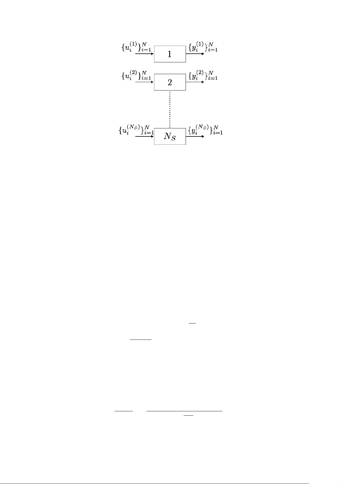
Data Driv en Estimation of Sto c hastic Switc hed Linear Systems of Unkno wn Order T uhin Sark ar Alexander Rakhlin Munther Dahleh ∗ No vem b er 4, 2021 Abstract W e address the problem of learning the parameters of a mean square stable switched linear systems (SLS) with unknown latent space dimension, or or der , from its noisy input–output data. In particular, w e fo cus on learning a go od lo w er order approximation of the underlying mo del allow ed by finite data. Motiv ated b y subspace-based algorithms in system theory , we construct a Hankel-lik e matrix from finite noisy data using ordinary least squares. Such a formulation circumv ents the non-con vexities that arise in system identification, and allows for accurate estimation of the underlying SLS as data size increases. Since the mo del order is unknown, the key idea of our approach is mo del order selection based on purely data dep enden t quantities. W e construct Hankel-lik e matrices from data of dimension obtained from the order selection pro cedure. By exploiting to ols from theory of mo del reduction for SLS, w e obtain suitable approximations via singular v alue decomp osition (SVD) and show that the system parameter estimates are close to a balanced truncated realization of the underlying system with high probability . 1 In tro duction Finite time system identification is an imp ortant problem in the context of con trol theory , times series analysis and rob otics among man y others. In this w ork, we fo cus on parameter estimation and model appro ximation of switched linear systems (SLS), whic h are described by x k +1 = A θ k x k + B u k + η k +1 (1) y k = C x k + w k Here at time k , x k ∈ R n , y k ∈ R p , u k ∈ R m are the latent state, output and input respectively . θ k ∈ { 1 , 2 , . . . , s } is the discrete state, mode or switc h with η k , w k b eing the pro cess and output noise resp ectiv ely . W e assume that { θ k } ∞ k =1 is an i.i.d pro cess with P ( θ k = i ) = p i . The goal is to learn ( C, { p i , A i } s i =1 , B ) from observ ed data { y k , u k , θ k } N k =1 when the laten t space dimension n is unkno wn. In man y cases n > p, m and it b ecomes difficult to find suitable parametrizations that allow for pro v ably efficien t learning. F or the sp ecial case of L TI systems, i.e. , s = 1, these issues w ere discussed in detail in [ 1 ]. It was suggested there that one can learn lo wer order approximations of the original system from finite noisy data. T o motiv ate the study of such approximations, consider the following example: Example 1. L et s = 2 , p i = 0 . 5 , | γ | < 1 . Consider M 1 = { C, A 1 ∈ R n × n , B } , M 2 = { C, A 2 ∈ R n × n , B } given by B =      0 . . . 0 1      , C = B > , A 1 =      0 0 . . . 0 0 0 . . . 0 . . . . . . . . . . . . 0 . . . 0 γ      A 2 =       0 1 . . . 0 0 0 . . . 0 . . . . . . . . . . . . a 0 . . . 0       (2) ∗ TS,AR,MD are with Massach usetts Institute of T echnology , Cambridge, MA 02139 (email: tsarkar,rakhlin, dahleh@mit.edu ) Assume that na  1 . This SLS is of or der n , which may b e lar ge. However, it c an b e suitably mo dele d by a lower dimensional SLS (“effe ctive” or der is ≤ 2 and c an b e che cke d by a simple c omputation of { C A i A j B } 2 i,j =1 ). In fact, the SLS with p ar ameters B = C = 1 and A 1 = γ , A 2 = 0 gener ate the same output. The previous example suggests that in many cases the true order is not imp ortant; rather a low er order mo del exists that appro ximates the true system w ell. F urthermore, finite noisy data limits the complexity of mo dels that can be effectively learned (See discus sion in [ 2 ]). The existence of an “effectiv e” low er order and finite data length motiv ate the question of finding “go o d” low er dimensional approximations of the underlying mo del from finite noisy data. Classical system iden tification results pro vide asymptotic guaran tees for learning from data [ 3 ]. Finite sample analysis for linear system iden tification has also been studied in [ 4 ]. How ever, when considering finite noisy data problems suc h as those o ccurring for example in reinforcemen t learning, these results are either to o p essimistic (finite time bounds) due to a worst case analysis or inapplicable due to their asymptotic nature. In this work, we fo cus on estimation of stochastic switched linear systems when the mo del order is unknown. W e b elieve such a discussion is imp ortant in tw o aspects: first, typically the hidden state x k in Eq. (1) is unobserved. Second, as discussed in Example 2 although the true system ma y b e of a high order, it could also b e “well” appro ximated by a m uch low er order system. 1.1 Related W ork The study of switc hed linear systems (SLS) has attracted a lot of atten tion [ 5 , 6 , 7 ] to name a few. These hav e b een used in neuroscience to mo del neuron firing [ 8 ], mo deling the stock index [ 9 ] and more generally approximate non–linear pro cesses [ 10 ] with reasonable accuracy . The theoretical aspects of SLS (deterministic or sto c hastic) hav e b een studied on several fronts: realizabilit y , mo del reduction and iden tification from data. The problem of realization, i.e. , whether there exists a SLS that satisfies the given data (in the noiseless case), has b een studied in [ 11 , 12 , 13 ] and references therein. Sp ecifically , [ 11 ] pro vides a purely algebraic view of realization where the switc hing is a function of exogenous discrete input symbols. The authors in [ 12 ] consider the case when discrete ev ents are external inputs and there are linear reset maps that reset the state after switching. They pro vide necessary and sufficien t conditions for existence of a SLS that generates the giv en output data in response to certain inputs. The question of minimalit y via the rank of a generalized Hank el matrix is also discussed there. The results for SLS there imply the classical ones for linear time in v ariant (L TI) systems. These ideas are further extended to generalized bilinear systems in [13]. Hybrid systems, where systems hav e a contin uous state and discrete state, are a generalization of SLS and piecewise linear ARX (PW ARX) systems. Man y approaches ha v e b een devised for hybrid system iden tification: supp ort v ector regression(SVR)-based approach [ 14 ], the clustering-based approach [ 15 ], the mixed in teger programming based approac h [ 16 ], the Bay esian approac h [ 17 ], the b ounded error approac h [ 18 , 19 ], sparse optimization approac h [ 20 ] and the algebraic approach [ 21 ]. An underlying assumption in man y of these approac hes is the assumption that an upper bound on the mo del order (dimension of contin uous state) is kno wn apriori. F urthermore, approaches such as mixed integer linear programming, clustering and SVR do not assume that the switch sequences are observ ed. Consequently , this causes the identification problem to be NP-hard. In con trast, we assume that the switc h sequence is exogenous and known. Ho wev er, we do not require that an upp er b ound on the mo del order be known. F rom a system theory p ersp ective, mo del approximation of SLS has b een very well studied [ 22 , 23 , 24 ]. These metho ds mimic balanced truncation–like metho ds for mo del reduction and pro vide error guarantees b et w een the original and reduced system. Despite substan tial work on realization theory , identification and mo del reduction of SLS, there is little work on data driven approaches of SLS identification when mo del order is unkno wn, even when the switches are observ ed. There is recen t interest from the machine learning comm unity in data-driv en con trol and non- asymptotic analysis. In this context, L TI system identification from finite noisy data for the purpose of con trol has play ed a cen tral role [ 1 , 25 , 26 , 27 , 28 ]. Sp ecifically , [ 1 ] study data driv en approaches to learning reduced order appro ximations of the original mo del. F urthermore, [ 1 ] studies L TI system iden tification when mo del order is unknown which is ac hieved by constructing low-order appro ximations of the underlying system from noisy data, where the order grows as the length of data increases. On the other hand, [ 29 ] study the Lo ewner framew ork for learning state space mo dels directly from data and in principle, allo ws a trade-off b etw een accuracy and complexit y of mo del learned. How ever, the authors do not assume the presence of noise in the data. 2 Preliminaries Throughout the pap er, we will refer to the switc hes linear system (SLS) with dynamics as Eq. (1) b y M = ( C, { A i , p i } s i =1 , B ). F urthermore, the SLS M 1 = ( C, { A i , p i } s i =1 , B ) is equiv alent to M 2 = ( C S − 1 , { S A i S − 1 , p i } s i =1 , S B ) for an y fixed S . F or a matrix A , let σ i ( A ) be the i th singular v alue of A with σ i ( A ) ≥ σ i +1 ( A ). F urther, σ max ( A ) = σ 1 ( A ) = σ ( A ). Similarly , we define ρ i ( A ) = | λ i ( A ) | , where λ i ( A ) is an eigenv alue of A with ρ i ( A ) ≥ ρ i +1 ( A ). Again, ρ max ( A ) = ρ 1 ( A ) = ρ ( A ). W e define the Kronec k er pro duct of tw o matrices A, B as A ⊗ B . F or any matrix Z , define Z i : j,k : l as the submatrix including ro w i to j and column k to l . F urther, Z i : j, : is the submatrix including row i to j and all columns and a similar notion exists for Z : ,k : l . W e no w define stability of a SLS. Definition 1 ([ 30 ]) . SLS is me an–squar e stable if P s i =1 p i A i ⊗ A i is Schur stable, i.e., ρ ( P s i =1 p i A i ⊗ A i ) < 1 . Recall the SLS dynamics in Eq. (1) . Denote b y l j i = { θ j , θ j − 1 , . . . , θ i } ∈ [ s ] j − i +1 an arbitrary sequence of switches from i to j and A l j i : = A θ j A θ j − 1 . . . A θ i . F or t wo switch sequences { θ 2 , θ 1 } , { φ 2 , φ 1 } define a concatenation op erator ‘:’ as { θ 2 , θ 1 } : { φ 2 , φ 1 } = { θ 2 , θ 1 , φ 2 , φ 1 } . Then l i 1 : l j 1 is concatenation of l i 1 , l j 1 . It is clear that for any sequence of observ ed switches l N 1 , we hav e the corresp onding output y N of SLS in Eq. (1) as y N = N − 1 X j =2 C A θ N − 1 A θ N − 2 . . . A θ j B u j − 1 + C B u N − 1 | {z } Input driven terms + N − 1 X j =2 C A θ N − 1 A θ N − 2 . . . A θ j η j − 1 + C η N − 1 + w N | {z } Noise terms (3) A measure of distance b etw een t wo switched linear systems with probabilistic switc hes is the sto chastic L 2 gain given by Definition 2 (Definition 2 . 2 in [ 22 ]) . L et the noise { η k , w k } ∞ k =1 = 0 . L et θ = ( θ 1 , θ 2 , . . . ) ∈ [ s ] ∞ , u = ( u 1 , u 2 , . . . ) ∈ R ∞ and y ( θ,u ) M , y ( θ,u ) M r ∈ R ∞ b e the output se quenc e, in r esp onse to input u and switch se quenc e θ , of system M and M r r esp e ctively. Then the sto chastic L 2 distanc e b etwe en M and M r denote d by ∆ M ,M r is ∆ 2 M ,M r = sup || u || 2 ≤ 1 E θ [ || y ( θ,u ) M − y ( θ,u ) M r || 2 2 ] Similar to linear time inv arian t systems, we will define the doubly infinite system Hankel matrix for SLS. T his can b e done for example as in [ 31 ]. T o summarize, ev ery sequence l N 1 has a unique index, i.e. , there exists a map L ( · ) which tak es as argumen t a switc h sequence and outputs an integer: L ( l N 1 ) = θ N s N − 1 + . . . + θ 1 with N = 0 = ⇒ L ( l N 1 ) = 0. Then the p ( s N +1 − 1 s − 1 ) × m ( s N +1 − 1 s − 1 ) Hankel–lik e matrix can b e constructed as follo ws: define r = pL ( l i 1 ) , s = mL ( l j 1 ) [ H ( N ) ] r +1: r + p,s +1: s + m = p p l i 1 : l j 1 C A l i 1 : l j 1 B (4) ∀ 0 ≤ i, j ≤ N − 1. Then H ( ∞ ) is the doubly infinite system Hankel matrix for SLS. It is a well kno wn fact that H ( ∞ ) exists and is w ell defined whenev er p i A i ⊗ A i is Sch ur stable. Define H ( N ) k as [ H ( N ) k ] pL ( l i 1 )+1: pL ( l i 1 )+ p,mL ( l j 1 )+1: mL ( l j 1 )+ m = [ H ( N ) ] pL ( l i 1 : { k } )+1: pL ( l i 1 : { k } )+ p,mL ( l j 1 )+1: mL ( l j 1 )+ m (5) Example 2. L et s = 2 . Then L ( φ ) = 0 , L ( { 1 } ) = 1 , L ( { 2 } ) = 2 , L ( { 1 , 1 } ) = 3 , L ( { 1 , 2 } ) = 4 , . . . . As a r esult H ( ∞ ) =           C B √ p 1 C A 1 B √ p 2 C A 2 B p p 2 1 C A 2 1 B . . . √ p 1 C A 1 B p p 2 1 C A 2 1 B √ p 1 p 2 C A 1 A 2 B p p 3 1 C A 3 1 B . . . √ p 2 C A 2 B √ p 1 p 2 C A 2 A 1 B p p 2 2 C A 2 2 B p p 2 p 2 1 C A 2 A 2 1 B . . . p p 2 1 C A 2 1 B p p 3 1 C A 3 1 B p p 2 1 p 2 C A 2 1 A 2 B p p 4 1 C A 4 1 B . . . √ p 1 p 2 C A 1 A 2 B p p 2 1 p 2 C A 1 A 2 A 1 B p p 1 p 2 2 C A 1 A 2 2 B p p 3 1 p 2 C A 1 A 2 A 2 1 B . . . . . . . . . . . . . . . . . .           (6) H ( ∞ ) k = √ p k           C A k B √ p 1 C A k A 1 B √ p 2 C A k A 2 B . . . √ p 1 C A 1 A k B p p 2 1 C A 1 A k A 1 B √ p 1 p 2 C A 1 A k A 2 B . . . √ p 2 C A 2 A k B √ p 1 p 2 C A 2 A k A 1 B p p 2 2 C A 2 A k A 2 B . . . p p 2 1 C A 2 1 A k B p p 3 1 C A 2 1 A k A 1 B p p 2 1 p 2 C A k A 2 1 A 2 B . . . √ p 1 p 2 C A 1 A 2 A k B p p 2 1 p 2 C A 1 A 2 A k A 1 B p p 1 p 2 2 C A k A 1 A 2 A k A 2 B . . . . . . . . . . . . . . .           (7) Note that in the sp ecial case of s = 1, p 1 = 1 and H ( ∞ ) b ecomes the usual doubly infinite system Hank el matrix for L TI systems. F urthermore, the order of M is giv en by rank( H ( ∞ ) ). Definition 3 ([ 23 ]) . L et H ( ∞ ) = U Σ V > b e the doubly infinite system Hankel matrix for SLS M , wher e Σ ∈ R n × n ( n is the mo del or der) and H ( ∞ ) k b e as in Eq. (5) . Then for any r ≤ n , the r –or der b alanc e d trunc ate d mo del p ar ameters ar e given by C ( r ) = [ U Σ 1 / 2 ] 1: p, 1: r , A ( r ) k = √ p k [Σ − 1 / 2 U > ] 1: r, : H ( ∞ ) k [ V Σ − 1 / 2 ] : , 1: r , B ( r ) = [Σ 1 / 2 V > ] 1: r, 1: m . F or r > n , the r –or der b alanc e d trunc ate d mo del p ar ameters ar e the n –or der trunc ate d mo del p ar ameters. The stability of balanced truncated mo dels is discussed in [ 24 ]. W e briefly summarize it in Section B. Remark 1. Note that A ( r ) k for k ∈ [ s ] c an also b e obtaine d in the same fashion as b alanc e d trunc ate d mo dels, sp e cific al ly A r , for L TI systems in [1]. We chose this version b e c ause it is e asier to r epr esent. Definition 4 ([32]) . We say a r andom ve ctor v ∈ R d is sub gaussian with varianc e pr oxy τ 2 if sup || θ || 2 =1 sup p ≥ 1 n p − 1 / 2 ( E [ |h v , θ i| p ]) 1 /p o = τ and E [ v ] = 0 . We denote this by v ∼ subg ( τ 2 ) . Finally , for tw o matrices M 1 ∈ R l 1 × l 1 , M 2 ∈ R l 2 × l 2 with l 1 < l 2 , M 1 − M 2 , ˜ M 1 − M 2 where ˜ M 1 =  M 1 0 l 1 × l 2 − l 1 0 l 2 − l 1 × l 1 0 l 2 − l 1 × l 2 − l 1  . W e use non-asymptotic big-oh notation, writing f = O ( g ) if there exists a numerical constant such that f ( x ) ≤ c · g ( x ) and f = e O ( g ) if f ≤ c · g max { log g , 1 } . 3 Con tributions In our w ork w e study the case when noisy { y k , u k , θ k } N k =1 is observed and we w ould like to learn ( C, { A i , p i } s i =1 , B ) from observed data when n is unkno wn. Such a case is relev ant when the switc hes are exogenous but not a control input. The contributions of this pap er can be summarized as follows: • W e pro vide the first sample complexit y guarantees for SLS iden tification when the underlying order is unknown. W e use to ols from finite sample analysis and model reduction theory to deriv e algorithms that recov er system parameters when only finite noisy data is presen t. • Cen tral to parameter estimation is estimating the SLS Hankel matrix. A critical step of our algorithm is mo del selection. W e deriv e a data dependent model selection rule that enables us to construct finite time estimators of the SLS Hank el matrix. The data dep endent rule creates a balance betw een the estimation error and truncation error of the finite time estimator. Sp ecifically , if N S are the num b er of samples then we show that ||H ( ∞ ) − b H ( b N ) || F ≤ e O  N − ∆ s / 2 S  , where H ( ∞ ) , b H ( b N ) are the SLS Hankel matrix and finite time estimator resp ectively , ∆ s > 1 and e O ( · ) hides only system dep enden t constan ts. This sho ws that as N S → ∞ the finite time estimator is consistent. • Using to ols from systems theory , i.e. balanced truncation, we obtain parameter estimates by a singular v alue decomp osition (SVD) of the finite time estimator b H ( b N ) . By using a v arian t of W edin’s theorem w e sho w that the parameter estimates are close to a low order balanced truncation of the true SLS. W e sho w that this a form of subspace recov ery where reco v ery of a low er order appro ximation dep ends only on the singular v alue of the Hank el matrix corresp onding to that order and not the lo wer singular v alues, i.e. , let M r = ( C ( r ) , { A ( r ) i } s i =1 , B ( r ) ) be the r -order balanced truncated approximation of the true SLS and c M r = ( b C ( r ) , { b A ( r ) i } s i =1 , b B ( r ) ) b e the estimates of our algorithm then || M r − c M r || ≤ e O  r ∨ 1 √ σ r  · N − ∆ s / 2 S  where || · || is an appropriately defined norm and σ i are the SLS Hank el singular v alues. 4 Problem F orm ulation and Discussion 4.1 Data Generation Let M n b e the class of n -dimensional mean-squared SLS mo dels, i.e. , M n = ( ( C, { A i , p i } s i =1 , B ) | A i ∈ R n × n , ρ s X i =1 p i A i ⊗ A i ! < 1 ) . Assume that the data is generated by M = ( C, { A i , p i } s i =1 , B ) ∈ M n for some unknown n . Supp ose w e observe the noisy output time series { y t ∈ R p × 1 } T t =1 and { θ t ∈ [ s ] } T t =1 in resp onse to chosen input series { u t ∈ R m × 1 } T t =1 . W e refer to this data generated by M as Z T = { ( u t , y t , θ t ) } T t =1 . W e enforce the follo wing assumptions on M Assumption 1. { η t , w t } ∞ t =1 ar e i.i.d subg (1) . F urthermor e x 0 = 0 almost sur ely. We wil l only sele ct inputs { u t } T t =1 that ar e N (0 , I ) . Assumption 2. The numb er of distinct switches s is known. F urthermor e, ther e exists β > 0 such that sup N ≥ 0 n || C A l N 1 B || 2 F , || C A l N 1 || 2 F o ≤ β 2 , sup i ∈ [ s ] || A i || 2 ≤ γ . The goal is to iden tify { C, { p i , A i } s i =1 , B } from data { y k , u k , θ k } ∞ k =1 when n (or its upp er b ound) is unkno wn. W e next describ e the problem setup. W e assume that the switc hed linear system can b e restarted multiple times as sho wn in Fig. 1. Sp ecifically , the data collection pro cess is as follows: eac h SLS system, or sample, t ∈ [ N S ] is allow ed to run for a length of time N , also known as the rollout length. W e define N S as the sample complexity . Let θ ( t ) k , y ( t ) k , u ( t ) k denote the switc h, output and input resp ectively at rollout time k for sample t . Now define the set N m i as N m l : = { ( t, k ) | ( θ ( t ) k + l − 1 , θ ( t ) k + l − 2 , . . . , θ ( t ) k ) = m l ∈ [ s ] l } (8) N m l is the set of occurrences of the switch sequence m l with N m l = |N m l | . W e briefly des cribe the in tuition b ehind the setup in Fig. 1. Figure 1: System Setup 4.2 Significance of N and N S Our algorithm can b e in terpreted as an extension to the approac h describ ed for L TI systems in [ 1 ]. Ho wev er, the main difference b et w een the L TI Hankel matrix and SLS Hank e l matrix is that the dimension of the SLS Hankel grows exp onen tially in the rollout length in contrast to the linear gro wth for L TI systems. The reason b ehind this is the following: at an y time i an y one of s switc hes may b e observed, as a result if a SLS is allow ed to run for N steps, the total n umber of switc h sequences p ossible is s N . T o correctly estimate the underlying model, one needs to estimate C A l 1: N B for each of the sequences l 1: N ∈ [ s ] N . A t a high level, rolling out the SLS allows us to understand its “mixing” prop erties, i.e. , for a given N w e observe noisy versions of C A l i 1 B for i ∈ [ N ]. { C A l i 1 B } N i =1 is then used to construct the SLS Hankel matrix. F rom this p ersp ective, a large v alue of N , or rollout length, giv es us more information ab out the true SLS. Ho w ev er, because the observ ations obtained from a single SLS (or tra jectory) are noisy w e w ould lik e multiple i.i.d copies of the SLS (or tra jectories) to “av erage” out the noise and reco v er C A l i 1 B . As discussed b efore for a rollout length of N , we need to estimate s N parameters to construct the Hankel matrix, therefore to ensure that we do not hav e more parameters than independent samples w e need to ensure that s N < N S . This in tro duces a trade-off: N cannot b e to o small as that could lead to high truncation of the Hankel matrix and it should not b e too large compared to N S as that will induce error in estimation of the Hankel matrix parameters. In view of this trade-off, an imp ortant step in our SLS Hank el estimation (Algorithm 2) is that we set C A l i 1 B = 0 for sequences l i 1 that do not occur “often enough”. T o that end, define N up = inf  l    N l l 1 < 2  m + log 2 s l δ  ∀ l l 1 ∈ [ s ] l  s h = s h +1 − 1 s − 1 . (9) N up is the minim um length for which the num b er of o ccurrences of al l switch sequences of that length do es not exceed a certain pre-determined threshold. If the SLS is allow ed to “roll-out” b ey ond this length w e do not ha ve enough samples to accurately learn the parameters corresponding to that length. W e next sho w that N up gro ws at most logarithmically with the num b er of samples N S . This is inline with the intuition that when N S samples are present we should b e able to learn O ( N S ) parameters. Prop osition 1. F or N up that is the output of Algorithm 1 we c an show with pr ob ability at le ast 1 − δ that N up log N up ≥ log 2 m + log N S + log log (1 /δ ) log 1 p max ! wher e p max = max 1 ≤ i ≤ s p i . The pro of of this can b e found in Section C.1. Algorithm 1 Choosing rollout length Input Input: { u ( l ) m } l = N S ,m = N S l =1 ,m =1 Output N up 1: for i = 1 , . . . , N S do 2: Collect output ( y ( l ) i , θ ( l ) i ) l = N S l =1 3: if ∃ l i 1 suc h that N l i 1 ≥ 2( m + log (2 s i /δ )) then 4: con tinue 5: else 6: N up = i − 1 7: break 8: Return : N up , { u ( l ) m , y ( l ) m , θ ( l ) m } l = N S ,m = N up l =1 ,m =1 5 Algorithmic Details The goal is to learn the infinite Hankel-lik e matrix H ( ∞ ) , from which w e can obtain the system parameters ( C, { A i , p i } s i =1 , B ) b y balanced truncation. How ever due to the presence of only finite noisy data w e will instead construct finite time estimators of H ( ∞ ) from data. W e will show that this estimator approac hes H ( ∞ ) as the length of data increases. F urthermore, for finite N S w e can obtain “go o d” lo w er order approximations of the true SLS from our estimator. Broadly , our algorithmic approac h can b e encapsulated in Fig 2. Figure 2: Here T = N × N S , the total num b er of observ ations av ailable. Let M b e the true data generating SLS where Z T = { u ( l ) m , y ( l ) m , θ ( l ) m } l = N S ,m = N l =1 ,m =1 and M r b e a go o d r -order approximation of M obtained by a pro cedure H . Let c M r ( T ) b e a r -order mo del estimate obtained by algorithm b H T whic h takes as input Z T . Since n is apriori unkno wn an y parametrization of the mo del may lead to inconsisten t estimators. Instead, for an y T w e estimate SLS c M r ( T ), that is “close” to M r . As T → ∞ , r → n and c M r ( T ) approaches M . The key steps of our algorithm are summarized b elow. (a) Hank el submatrix estimation: Estimating H ( l ) for ev ery 1 ≤ l ≤ N . W e refer to these estimators as { b H ( l ) } N l =1 . This is ac hiev ed by estimating Θ l i 1 = C A l i 1 B for every switch sequence l i 1 ∈ [ s ] i where i ∈ [ N ]. (b) Mo del selection: F rom the estimators { b H ( l ) } N l =1 select b H ( b N ) in a data dependent wa y suc h that it “b est” estimates H ( ∞ ) . (c) P arameter estimation: W e do a singular v alued decomposition of b H ( b N ) to obtain parameter estimates for a b N -order balanced truncated model. W e summarize some of the key notation b elo w. 5.1 Hankel submatrix estimation T o estimate the Hankel submatrix w e learn eac h of its entries by linear regression, i.e. , for ev ery switch sequence l i 1 ∈ [ s ] i , w e wan t to learn Θ l i 1 = C A l i 1 B and its probability p l i 1 of occurrence. This is sho wn in Algorithm 2. N S : Sample complexit y s d = s d +1 − 1 s − 1 N up : inf n l    N l l 1 < α  m + log 2 s l δ  ∀ l l 1 ∈ [ s ] l o m : Input dimension, p : Output dimension δ : Error probability ρ max : ρ ( P s i =1 p i A i ⊗ A i ) µ ( d ) = √ d ( d log (3 s/δ ) + p log (5 β d ) + m ) α ( d ) = µ ( d ) q 2 s d · d 2 N S ∆ s = log (1 /ρ max ) log ( s/ρ max ) T able 1: Summary of constants Algorithm 2 Regression Estimates Input Data: { u ( l ) m , y ( l ) m , θ ( l ) m } l = N S ,m = N up l =1 ,m =1 Output Estimates: b H ( N ) , { b p i } s i =1 1: N = N up 2: for i = 1 , . . . , N do 3: if N l i 1 ≥ 2( m + N log 2 s δ ) then 4: b Θ l i 1 = arg inf Θ P ( t,k ) ∈N l i 1 || y ( t ) k − Θ u ( t ) k || 2 F 5: else 6: b Θ l i 1 = 0 7: b p l i 1 = ( N l i 1 N S ( N − i +1) , if i > 0 1 , otherwise 8: for a = 0 , 1 , . . . , N do 9: b = N − a 10: [ b H ( N ) ] pL ( l a 1 )+1: pL ( l a 1 )+ p,mL ( l b 1 )+1: mL ( l b 1 )+ m = q b p l a 1 : l b 1 b Θ l a 1 : l b 1 (10) 11: Return : b H ( N ) , { b p i } s i =1 . Our next result b ounds the error rates obtained from the regression. The pro of of this follows standard analysis in statistical learning literature such as [33]. Prop osition 2. L et N b e the r ol lout length. Fix δ > 0 and se quenc e l i 1 ∈ [ s ] i . L et b Θ l i 1 b e the fol lowing solution b Θ l i 1 = arg inf Θ X ( t,k ) ∈N l i 1 || y ( t ) k − Θ u ( t ) k || 2 F wher e { u ( t ) k } ∞ t,k =1 ar e i.i.d isotr opic Gaussian (or isotr opic subg (1) ) r andom variables. Then whenever q N l i 1 ≥ c  √ m + p N log (6 s/δ )  we have with pr ob ability at le ast 1 − δ that || C A l i 1 B − b Θ l i 1 || F ≤ 10 min ( √ p, √ m ) · β s µ 2 ( N ) N l i 1 . (11) Her e c is an absolute c onstant. F urthermor e, E [ N l i 1 ] = p l i 1 N S ( N − i + 1) . Pr o of. The pro of of the first part can b e found in the appendix as Prop osition 11. The details are standard in statistical learning theory and require applications of Bernstein-type inequalities. T o see that b p l i 1 : l j 1 is an unbiased estimator for p l i 1 : l j 1 , recall the exp eriment set up: we run N S iden tical samples of the SLS for length N . Then for each sample i ≤ N S , any sequence l k 1 can start at p osition 1 , 2 , . . . , N − k + 1. Th us for the sample i the n um b er of o ccurrences of l k 1 is giv en b y P N − k +1 l =1 1 ( i ) { l k 1 starts at p osition l } , then N l k 1 is given by N l k 1 = N S X i =1 N − k +1 X l =1 1 ( i ) { l k 1 starts at p osition l } (12) and by linearity of exp ectation it is clear that E [ N l k 1 ] = p l k 1 N S ( N − k + 1). It is clear from Prop osition 2 that b p l i 1 is an unbiased estimator of p l i 1 b ecause E [ b p l i 1 ] = E [ N l i 1 ] N S ( N − i + 1) = p l i 1 An imp ortant feature of this algorithm is that when we hav e less data for a certain switc h sequence l i 1 , i.e. , N l i 1 < 2( m + N log 2 s δ ) w e simply set the parameter corresp onding to the switch sequence to zero. The reason b eing that when the o ccurrences of a particular switch sequence is lo w, regression cannot b e used to obtain reliable estimates. On the other hand, setting these parameters to zero does not lead to a high estimation error, whic h we sho w in Theorem 1. The reason is that in the Hankel matrix eac h en try C A l i 1 B is scaled by its probability of o ccurrence √ p l i 1 , as a result for lo w probability sequences the estimation error also remains low. Then we hav e the following estimation error upper b ound, Theorem 1. Fix δ > 0 and N . We have with pr ob ability at le ast 1 − δ , || b H ( N ) − H ( N ) || 2 F ≤ 2 β 2  N 2 N S  s N · µ 2 ( N ) = β 2 α 2 ( d ) . Her e s k = s k +1 − 1 s − 1 . The proof of this result can be found in Prop osition 13 in the app endix. Theorem 1 provides a finite time error b ound in estimating H ( N ) using Algorithm 2 for any fixed N . The b ound dep ends on quantities that are known apriori. This will be critical in designing a data dep endent rule for mo del selection. 5.2 Mo del Selection A t a high level, we w ant to choose b H ( b N ) from { b H ( l ) } N up l =1 suc h that b H ( b N ) is a go o d estimator of H ( ∞ ) . Our idea of model selection is motiv ated b y [34]. F or any b H ( l ) , the error from H ( ∞ ) can b e broken as: || b H ( l ) − H ( ∞ ) || F ≤ || b H ( l ) − H ( l ) || F | {z } =Estimation Error + ||H ( l ) − H ( ∞ ) || F | {z } =T runcation Error . The size of b H ( l ) is made equal to H ( ∞ ) b y padding it with zeros. W e would like to select a l = b N suc h that it balances the truncation and estimation error in the following w a y: c 2 · Upp er b ound ≥ c 1 · Estimation Error ≥ T runcation Error (13) where c i are absolute constants. Suc h a balancing ensures that || b H ( l ) − H ( ∞ ) || F ≤ c 2 · (1 /c 1 + 1) · Upp er b ound . (14) Note that such a balancing is possible b ecause the estimation error increases as l gro ws and truncation error decreases with l . F urthermore, a data dep endent upp er bound for estimation error can b e obtained from Theorem 1. Unfortunately ( C, { A i } s i =1 , B ) are unknown and it is not immediately clear on how to obtain such a b ound for truncation error. T o ac hieve this, w e first define a truncation error proxy , i.e. , how muc h do we truncate if a specific b H ( l ) is used. F or a given l , we look at || b H ( l ) − b H ( d ) || F for N up ≥ d ≥ l . This measures the additional error incurred if we choose b H ( l ) as an estimator for H ( ∞ ) instead of b H ( d ) for d > l . Then w e pic k b N as follo ws: b N : = inf ( l      || b H ( d ) − b H ( l ) || F ≤ β ( α ( d ) + 2 α ( l )) ∀ N up ≥ d ≥ l ) . (15) where α ( d ) is from T able 1. A k ey step will b e to show that for an y d ≥ l , whenev er || b H ( d ) − b H ( l ) || F ≤ cβ · α ( d ) ensures that || b H ( l ) − H ( ∞ ) || F ≤ cβ · α ( d ) and || b H ( d ) − H ( ∞ ) || F ≤ cβ · α ( d ) and there is no gain in choosing a larger Hankel submatrix estimate. By pic king the smallest l for whic h suc h a prop erty holds for all larger Hank el submatrices, we ensure that a regularized mo del is estimated that “agrees” with the data. The model selection algorithm is summarized in Algorithm 3. Algorithm 3 Choice of b N Output b H ( b N ) , b N 1: s d , α ( d ) from T able 1. 2: b N = inf n l    || b H ( d ) − b H ( l ) || F ≤ β (2 α ( d ) + α ( l )) o . 3: return b H ( b N ) , b N First we show that b N , i.e. , the output of Algorithm 3 do es not grow strongly with N S . Using this fact, we will show that b H ( b N ) is a go o d finite time estimator of H ( ∞ ) . Theorem 2. Assume that N S ≥  N up · c ( n ) ρ max (1 − ρ max ) · log N S  log (1 /p max ) log (1 /ρ max ) wher e c ( n ) is a c onstant that dep ends on m, n, p only. Then we have with pr ob ability at le ast 1 − δ that || b H ( b N ) − H ( ∞ ) || 2 F = e O ( N − ∆ s S ) . Pr o of. The pro of details are giv en in Prop osition 18. W e sk etch the proof here. First step is to show that there exists N ∗ suc h that, for N S that satisfies the conditions of the Theorem, we hav e T runcation Error ≤ Estimation Error and then sho wing that the estimation error decays with N S (Prop osition 16). The final step is to show that b N ≤ N ∗ , and using subadditivit y to sho w that || b H ( b N ) − H ( ∞ ) || F also decays with N S . Theorem 2 gives us an error b ound on the estimation of H ( ∞ ) that decays to zero as the num b er of samples increase via a metho d of mo del selection from data dep enden t quantities only . In the following section we will use this data dependent error bound to construct parametric estimates. F urthermore, note the sp ecial case of s = 1 (L TI systems). W e find that ∆ s = 1 when s = 1, i.e. , the error rate is e O ( N − 1 S ). This is exactly equal to the error rate obtained for L TI systems (See Theorem 5.2 in [1]). 5.3 Parameter Estimation Finally , to obtain the system parameters of the SLS w e use the following balanced truncation based algorithm. This inv olves a SVD of the Hank el matrix and the error b ounds can then be obtained by using a v ariant of W edin’s theorem. Algorithm 4 Learning SLS parameters Input b H ( b N ) : Hankel Estimator, { b p i } s i =1 : Probability estimates, r : Order Output System P arameters ( e C , { e A i } s i =1 , e B ) 1: Pad b H ( b N ) with zeros to mak e it of size 4 ps b N × 4 ms b N 2: b H ( b N ) 1:4 ps c N − p, 1:4 ms c N − m = b U b Σ b V > and 3: 4: b C ( r ) = [ b U b Σ 1 / 2 ] 1: p, 1: r , b B ( r ) = [ b Σ 1 / 2 b V > ] 1: r, 1: m 5: b A ( r ) i = b p − 1 / 2 i [ b Σ − 1 / 2 b U > ] 1: r, : b H ( N ) i [ b V b Σ − 1 / 2 ] : , 1: r 6: Return : ( b C ( r ) , { b A ( r ) i } s i =1 , b B ( r ) ) By Theorem 2 we know that b H ( b N ) is a “go o d” finite time estimator for H ( ∞ ) , i.e. , the error decays to zero as N S go es to infinit y . Since all low er order appro ximations of mean square stable SLS can b e obtained from H ( ∞ ) , b y using subspace p erturbation results w e will argue that these approximations can b e estimated from b H ( b N ) . T o state the main result we define a quantit y that measures the singular v alue w eigh ted subspace gap of a matrix S : Γ( S,  ) = q σ 1 max /ζ 2 1 + σ 2 max /ζ 2 2 + . . . + σ l max /ζ 2 l , where S = U Σ V > and Σ is arranged in to blocks of singular v alues suc h that in eac h blo ck i w e hav e sup j σ i j − σ i j +1 ≤  , i.e. , Σ =      Λ 1 0 . . . 0 0 Λ 2 . . . 0 . . . . . . . . . 0 0 0 . . . Λ l      where Λ i are diagonal matrices, σ i j is the j th singular v alue in the blo c k Λ i and σ i min , σ i max are the minim um and maximum singular v alues of block i resp ectiv ely . F urthermore, ζ i = min ( σ i − 1 min − σ i max , σ i min − σ i +1 max ) for 1 < i < l , ζ 1 = σ 1 min − σ 2 max and ζ l = min ( σ l − 1 min − σ l max , σ l min ) . Informally , the ζ i measure the singular v alue gaps b etw een eac h blo cks. It should b e noted that l , the num b er of separated blo cks, is a function of  itself. F or example: if  = 0 then the num b er of blocks corresp ond to the n umber of distinct singular v alues. On the other hand, if  is very large then l = 1. Let H ( ∞ ) = U Σ V > where Σ ∈ R n × n b ecause SLS is finite rank. Define Γ 0 : = sup τ ≥ 0 Γ(Σ , τ ) < ∞ . Theorem 3. L et N S satisfy the c onditions of The or em 2 and b d b e the numb er of non-zer o singular values of b H ( b N ) , M b e the true unknown mo del and ( C ( r ) , { A ( r ) i } s i =1 , B ( r ) ) b e its r -or der b alanc e d trunc ate d p ar ameters. Then, for r ≤ b d , ther e exists an ortho gonal tr ansformation Q such that with pr ob ability at le ast 1 − δ we have (a) If σ r ( H ( ∞ ) ) = Ω( N − ∆ s / 2 S ) then max  || b C ( r ) − C ( r ) Q || 2 , || b B ( r ) − Q > B ( r ) || 2  = e O Γ 0 · N − ∆ s / 2 S √ σ r ∨ r N − ∆ s / 2 S ! , || Q > A ( r ) Q − b A ( r ) || 2 = e O γ Γ 0 · N − ∆ s / 2 S √ σ r ∨ r N − ∆ s / 2 S ! . (b) If σ r ( H ( ∞ ) ) = o ( N − ∆ s / 2 S ) then max  || b C ( r ) − C ( r ) Q || 2 , || b B ( r ) − Q > B ( r ) || 2  = e O Γ 0 · N − ∆ s / 2 S √ σ r ∨ q r N − ∆ s / 2 S ! , || Q > A ( r ) Q − b A ( r ) || 2 = e O γ Γ 0 · N − ∆ s / 2 S √ σ r ∨ q r N − ∆ s / 2 S ! . The proof of Theorem 3 can b e found in Section C.5 in the appendix. W e note that when σ r is large then estimation error for the low er order appro ximation decays as e O ( N − ∆ s / 2 S ). On the other hand, if σ r is b elow a certain threshold then the error decays at a slow er rate of e O ( N − ∆ s / 4 S ). 6 Discussion In this w ork we provide finite sample error guaran tees for learning realizations of SLS when stability radius or order is unknown. Sp ecifically , we construct a finite dimensional Hankel–lik e matrix from finite noisy data that estimates H ( ∞ ) and obtain parameter estimates b y balanced truncation. The t wo key features of our algorithm are choosing the rollout length and the size of the Hankel–lik e matrix using data dep endent metho ds. The data dep endent metho ds carefully balance the estimation and truncation errors incurred. Under stated assumptions, we obtain O  q N − ∆ s S  finite time error rates which coincide with the optimal rates for L TI systems when s = 1. Due to the nature of the analysis w e b elieve that the results can b e easily extended to the case when { θ t } ∞ t =1 ev olution is more complex, for e.g.: state dep enden t or a marko v chain. F urthermore, we assume d in this pap er that the discrete switches are completely observ able. A potential future direction could b e to com bine these results with clustering based metho ds describ ed in [ 15 ] to build a more general framew ork of SLS iden tification. References [1] T. Sark ar, A. Rakhlin, and M. A. Dahleh, “Finite-time system identification for partially observed lti systems of unkno wn order,” arXiv pr eprint arXiv:1902.01848 , 2019. [2] S. R. V enk atesh and M. A. Dahleh, “On system identification of complex systems from finite data,” IEEE T r ansactions on Automatic Contr ol , vol. 46, no. 2, pp. 235–257, 2001. [3] L. Ljung and B. W ahlb erg, “Asymptotic prop erties of the least-squares method for estimating transfer functions and disturbance sp ectra,” A dvanc es in Applie d Pr ob ability , vol. 24, no. 2, pp. 412–440, 1992. [4] M. C. Campi and E. W ey er, “Finite sample properties of system iden tification metho ds,” IEEE T r ansactions on A utomatic Contr ol , v ol. 47, no. 8, pp. 1329–1334, 2002. [5] J. Ezzine and A. H. Haddad, “Controllabilit y and observ ability of hybrid systems,” International Journal of Contr ol , vol. 49, no. 6, pp. 2045–2055, 1989. [6] M. S. Branicky , “Introduction to h ybrid systems,” in Handb o ok of networke d and emb e dde d c ontr ol systems . Springer, 2005, pp. 91–116. [7] Z. Sun, Switche d line ar systems: c ontr ol and design . Springer Science & Business Media, 2006. [8] S. W. Linderman, A. C. Miller, R. P . Adams, D. M. Blei, L. Paninski, and M. J. Johnson, “Recurrent switc hing linear dynamical systems,” arXiv pr eprint arXiv:1610.08466 , 2016. [9] E. F ox, E. B. Sudderth, M. I. Jordan, and A. S. Willsky , “Bay esian nonparametric inference of switc hing dynamic linear mo dels,” IEEE T r ansactions on Signal Pr o c essing , vol. 59, no. 4, pp. 1569–1585, 2011. [10] R. L. W estra, M. P . Ralf, and L. Peeters, “Identification of piecewise linear models of complex dynamical systems,” IF AC Pr o c e e dings V olumes , vol. 44, no. 1, pp. 14 863–14 868, 2011. [11] R. L. Grossman and R. G. Larson, “An algebraic approac h to h ybrid systems.” [12] M. Petreczky and J. H. v an Sch upp en, “Realization theory for linear h ybrid systems,” IEEE T r ansactions on A utomatic Contr ol , v ol. 55, no. 10, pp. 2282–2297, 2010. [13] M. P etreczky and R. Vidal, “Realization theory for a class of sto chastic bilinear systems,” IEEE T r ansactions on A utomatic Contr ol , v ol. 63, no. 1, pp. 69–84, Jan 2018. [14] F. Lauer and G. Blo ch, “Hybrid system identification,” in Hybrid System Identific ation . Springer, 2019, pp. 77–101. [15] G. F errari-T recate, M. Muselli, D. Lib erati, and M. Morari, “A clustering technique for the identifi- cation of piecewise affine systems,” Automatic a , vol. 39, no. 2, pp. 205–217, 2003. [16] J. Roll, A. Bemporad, and L. Ljung, “Identification of piecewise affine systems via mixed-integer programming,” Automatic a , vol. 40, no. 1, pp. 37–50, 2004. [17] A. L. Juloski, S. W eiland, and W. Heemels, “A bay esian approach to identification of hybrid systems,” IEEE T r ansactions on Automatic Contr ol , vol. 50, no. 10, pp. 1520–1533, 2005. [18] A. Bemporad, A. Garulli, S. Paoletti, and A. Vicino, “A b ounded-error approach to piecewise affine system identification,” IEEE T r ansactions on Automatic Contr ol , vol. 50, no. 10, pp. 1567–1580, 2005. [19] N. Oza y , C. Lagoa, and M. Sznaier, “Robust iden tification of switched affine systems via moments- based conv ex optimization,” in Pr o c e e dings of the 48h IEEE Confer enc e on De cision and Contr ol (CDC) held jointly with 2009 28th Chinese Contr ol Confer enc e . IEEE, 2009, pp. 4686–4691. [20] L. Bak o, “Identification of switched linear systems via sparse optimization,” A utomatic a , v ol. 47, no. 4, pp. 668–677, 2011. [21] R. Vidal, Y. Ma, and S. Sastry , “Generalized principal comp onent analysis (gpca),” IEEE tr ansactions on p attern analysis and machine intel ligenc e , v ol. 27, no. 12, pp. 1945–1959, 2005. [22] G. Kotsalis, A. Megretski, and M. A. Dahleh, “Balanced truncation for a class of sto c hastic jump linear systems and model reduction for hidden mark ov mo dels,” IEEE T r ansactions on Automatic Contr ol , vol. 53, no. 11, pp. 2543–2557, 2008. [23] A. Birouc he, B. Mourllion, and M. Basset, “Model order-reduction for discrete-time switched linear systems,” International Journal of Systems Scienc e , vol. 43, no. 9, pp. 1753–1763, 2012. [24] M. Petreczky , R. Wisniewski, and J. Leth, “Balanced truncation for linear switched systems,” Nonline ar Analysis: Hybrid Systems , vol. 10, pp. 4–20, 2013. [25] T. Sark ar and A. Rakhlin, “How fast can linear dynamical systems be learned?” arXiv pr eprint arXiv:1812.0125 , 2018. [26] M. K. S. F aradon b eh, A. T ew ari, and G. Michailidis, “Finite time identification in unstable linear systems,” arXiv pr eprint arXiv:1710.01852 , 2017. [27] S. Oymak and N. Ozay , “Non-asymptotic identification of lti systems from a single tra jectory ,” arXiv pr eprint arXiv:1806.05722 , 2018. [28] M. Simc howitz, H. Mania, S. T u, M. I. Jordan, and B. Rech t, “Learning without mixing: T o wards a sharp analysis of linear system identification,” arXiv pr eprint arXiv:1802.08334 , 2018. [29] I. V. Gosea, M. Petreczky , and A. C. Antoulas, “Data-driv en mo del order reduction of linear switched systems in the lo ewner framew ork,” SIAM Journal on Scientific Computing , vol. 40, no. 2, pp. B572–B610, 2018. [30] O. L. V. Costa, M. D. F ragoso, and R. P . Marques, Discr ete-time Markov jump line ar systems . Springer Science & Business Media, 2006. [31] Q. Huang, R. Ge, S. Kak ade, and M. Dahleh, “Minimal realization problem for hidden marko v mo dels,” in 2014 52nd A nnual Al lerton Confer enc e on Communic ation, Contr ol, and Computing (A l lerton) . IEEE, 2014, pp. 4–11. [32] R. V ershynin, “High-dimensional probabilit y ,” 2019. [33] S. T u, R. Bo czar, A. Pac k ard, and B. Rec ht, “Non-asymptotic analysis of robust con trol from coarse-grained identification,” arXiv pr eprint arXiv:1707.04791 , 2017. [34] A. Goldenshluger, “Nonparametric estimation of transfer functions: rates of conv ergence and adaptation,” IEEE T r ansactions on Information The ory , vol. 44, no. 2, pp. 644–658, 1998. [35] R. V ershynin, “Introduction to the non-asymptotic analysis of random matrices,” arXiv pr eprint arXiv:1011.3027 , 2010. [36] M. Rudelson, R. V ershynin et al. , “Hanson-wrigh t inequality and sub-gaussian concentration,” Ele ctr onic Communic ations in Pr ob ability , vol. 18, 2013. A Probabilistic Inequalities Prop osition 3 ([35]) . L et M b e a r andom matrix. Then we have for any  < 1 and any w ∈ S d − 1 that P ( || M || > z ) ≤ (1 + 2 / ) d P ( || M w || > (1 −  ) z ) . Prop osition 4 ([ 32 ] Theorem 5.39) . L et U b e a T × d matrix whose r ows, { u i } T i =1 , ar e indep endent and isotr opic r andom ve ctors in R d , b elonging to subg ( τ 2 ) . Then whenever √ T ≥ cτ 2  √ d + p log (2 /δ )  , we have that with pr ob ability at le ast 1 − δ , 3 4 · I  T X i =1 u i u > i  5 4 · I , wher e c > 0 is a numeric al c onstant. Theorem 4 (Theorem 8.5 in [ 1 ]) . L et {F t } ∞ t =0 b e a filtr ation. L et { η t ∈ R m , X t ∈ R d } ∞ t =1 b e sto chastic pr o c esses such that η t , X t ar e F t me asur able and η t is F t − 1 -c onditional ly subg ( τ 2 ) for some L > 0 . F or any t ≥ 0 , define V t = P t s =1 X s X > s , S t = P t s =1 X s η > s +1 . Then for any δ > 0 , V  0 and al l t ≥ 0 we have with pr ob ability at le ast 1 − δ S > t ( V + V t ) − 1 S t ≤ 2 τ 2  log 1 δ + log det ( V + V t ) det ( V ) + m  . Theorem 5 (Theorem 2.1 [ 36 ]) . L et M b e a fixe d matrix. Consider a r andom ve ctor X such that E [ X i ] = 0 , E [ X 2 i ] = 1 and X ∼ subg ( L 2 ) . Then for any t ≥ 0 , we have P ( ||| AX || 2 − || A || F | ≥ t ) ≤ 2 · exp  − ct 2 L 4 || A || 2  . Prop osition 5 (Bernstein’s Inequalit y) . L et { X i } i =1 b e zer o me an r andom variables. Supp ose that | X i | ≤ M almost sur ely, for al l i . Then, for al l p ositive t , P ( | n X i =1 X i | > t ) ≤ exp − 1 2 t 2 P E [ X 2 j ] + 1 3 M t ! . (16) Recall that b p l k 1 = N l k 1 N S ( N − k + 1) = 1 N S N S X i =1 N − k +1 X l =1 1 ( i ) { l k 1 starts at l } ( N − k + 1) | {z } x i where 0 ≤ x i ≤ 1 and { x i } N S i =1 are i.i.d random v ariables. Since E [ x i ] = p l k 1 . W e can use Bernstein’s inequalit y on P N S i =1 ( x i − p l k 1 ). Note E [( x i − p l k 1 ) 2 ] ≤ p l k 1 . Then b y Bernstein’s inequality w e hav e Prop osition 6. Fix δ, N > 0 . F or al l se quenc es l k 1 with k ≤ N we have simultane ously with pr ob ability at le ast 1 − δ    N S X i =1 x i − p l k 1 N S    ≤ ( log s N δ , if log s N δ > p l k 1 N S q p l k 1 N S log s N δ , otherwise wher e s N = s N +1 − 1 s − 1 . Pr o of. First, we will sho w this high probabilit y b ound for a sp ecific sequence l k 1 and then w e will giv e the b ound for all sequences of length at most N b y using a union bound. F or a sp ecific sequence l k 1 w e hav e with probability at least 1 − δ ,    N S X i =1 x i − p l k 1 N S    ≤ ( log 1 δ , if log 1 δ > p l k 1 N S q p l k 1 N S log 1 δ , otherwise This is obtained from Proposition 5 where M = 1 and E [ X 2 j ] ≤ p l k 1 . Now, the total n umber of sequences is s N = s N +1 − 1 s − 1 . If we wan t, the preceding relation to hold simultaneously for all sequences then we hav e with probability at least 1 − s N δ that    N S X i =1 x i − p l k 1 N S    ≤ ( log 1 δ , if log 1 δ > p l k 1 N S q p l k 1 N S log 1 δ , otherwise for every sequence of length k ≤ N . By substituting δ → s − 1 N δ , w e get the desired the b ound. B Miscellaneous Results on Systems Theory Prop osition 7 (Similarit y Equiv alence) . Given the Hankel matrix H ( ∞ ) . If ( C, { A i , p i } s i =1 , B ) gener ates H ( ∞ ) then ( C S, { S − 1 A i S, p i } , S − 1 B ) gener ates H ( ∞ ) as wel l, i.e., ( C, { A i , p i } s i =1 , B ) is e quivalent to ( C S, { S − 1 A i S, p i } , S − 1 B ) in input-output b ehavior. Pr o of. The pro of follows from straigh tforw ard computation. Prop osition 8 (Stabilit y of balanced truncation) . Given a SLS M = ( C, { A i , p i } s i =1 , B ) and assume that the switches ar e indep endent. L et M r b e the r -or der b alanc e d trunc ate d mo del, then M r is me an-squar e d stable and ∆ M ,M r ≤ 2 s n X i = r +1 σ i wher e σ i is the i th singular value of H ( ∞ ) . Pr o of. Define ( e C i , e A i , e B i ) = ( √ p i C, √ p i A i , √ p i B ), then ρ ( P s i =1 e A i ⊗ e A i ) < 1, i.e. , the system with parameters M = { ( √ p i C, √ p i A i , √ p i B ) } s i =1 is strongly stable as in Definition 14 in [24]. F ollo wing that we use Lemma 12 and Theorem 6 in [24] to obtain stability and p erformance guarantees for the reduced system from [23]. Prop osition 9 (Proposition 14.2 in [1]) . L et H ( ∞ ) = U Σ V > , b H ( b N ) = b U b Σ b V > and ||H ( ∞ ) − b H ( b N ) || F ≤ . Define the r –or der b alanc e d trunc ate d p ar ameters C ( r ) : = [ U Σ 1 / 2 ] 1: p, 1: r , A ( r ) k : = √ p k [Σ − 1 / 2 U > ] 1: r, : H ( ∞ ) k [ V Σ − 1 / 2 ] : , 1: r , B ( r ) : = [Σ 1 / 2 V > ] 1: r, 1: m , and analo gously b C ( r ) , b A ( r ) k , B ( r ) for k ∈ [ s ] using b U , b Σ , b V . L et Σ b e arr ange d into blo cks of singular values such that in e ach blo ck i we have sup j σ i j − σ i j +1 ≤ χ for some χ ≥ 2 , i.e., Σ =      Λ 1 0 . . . 0 0 Λ 2 . . . 0 . . . . . . . . . 0 0 0 . . . Λ l      wher e Λ i ar e diagonal matric es and σ i j is the j th singular value in the blo ck Λ i . Then ther e exists an ortho gonal tr ansformation, Q , such that max  || b C ( r ) − C ( r ) Q || 2 , || b B ( r ) − Q > B ( r ) || 2  ≤ 2  q σ 1 /ζ 2 n 1 + σ n 1 +1 /ζ 2 n 2 + . . . + σ P l − 1 i =1 n i +1 /ζ 2 n l + 2 sup 1 ≤ i ≤ l p σ i max − q σ i min +  √ σ r ∧ √  = ζ , || Q > A ( r ) Q − b A ( r ) || 2 ≤ 4 γ · ζ / √ σ r . Her e sup 1 ≤ i ≤ l p σ i max − p σ i min ≤ χ √ σ i max r ∧ √ χr  and ζ n i = min ( σ n i − 1 min − σ n i max , σ n i min − σ n i +1 max ) for 1 < i < l , ζ n 1 = σ n 1 min − σ n 2 max and ζ n l = min ( σ n l − 1 min − σ n l max , σ n l min ) . C Pro ofs from the main pap er C.1 Pro of of Prop osition 1 Prop osition 10. F or N up define d in Eq. (9) we c an show with pr ob ability at le ast 1 − δ that N up log N up ≥ log 2 m + log N S + log log (1 /δ ) log 1 p max ! wher e p max = max 1 ≤ i ≤ s p i . Pr o of. By definition N up is the least l for which we hav e N l l 1 < 2  m + log 2 s l δ  ∀ l l 1 ∈ [ s ] l where s l = s l +1 − 1 s − 1 . Note from the first inequalit y of Prop osition 6 w e ha ve that for all sequences of length k , if N l k 1 ≤ 2 log s k +1 − 1 ( s − 1) δ , then it implies that with probabilit y at least 1 − δ w e get 2  m + log  s N up +1 − 1 ( s − 1) δ   ≥ p N up max · N S , whic h gives us that N up log N up ≥ log 2 m + log N S + log log (1 /δ ) log 1 p max ! . C.2 Pro of of Prop osition 2 Prop osition 11. Fix δ > 0 and se quenc e l i 1 ∈ [ s ] i . L et b Θ l i 1 b e the fol lowing solution b Θ l i 1 = arg inf Θ X ( t,k ) ∈N l i 1 || y ( t ) k − Θ u ( t ) k || 2 F wher e { u ( t ) k } ∞ t,k =1 ar e i.i.d isotr opic Gaussian (or subGaussian) r andom variables. Then whenever q N l i 1 ≥ c  √ m + p N log (6 s/δ )  we have with pr ob ability at le ast 1 − δ that || C A l i 1 B − b Θ l i 1 || F ≤ 10 min ( √ p, √ m ) · β s N N m l ·  log 3 s N δ + p log (5 β N ) + m  . (17) Her e N is the r ol lout length and c is an absolute c onstant. Pr o of. Recall y t as a function of { u l } t l =1 , y t = t − 1 X j =2 C A θ t − 1 A θ t − 2 . . . A θ j B u j − 1 + C B u t − 1 | {z } Input driven terms + t − 1 X j =2 C A θ t − 1 A θ t − 2 . . . A θ j η j − 1 + C η t − 1 + w t | {z } Noise terms , (18) then recall that N m l : = { ( t, k ) | ( θ ( t ) k + l − 1 , θ ( t ) k + l − 2 , . . . , θ ( t ) k ) = m l ∈ [ s ] l } for a switch sequence m l ∈ [ s ] l . According to our experiment set up we collect all data p oints corresponding to the switch sequence m l . Then we pick ( t, k ) ∈ N m l and b Θ m l =   X ( t,k ) ∈N m l y ( t ) k + l ( u ( t ) k − 1 ) >     X ( t,k ) ∈N m l u ( t ) k − 1 ( u ( t ) k − 1 ) >   + (19) Since the switch sequences are indep endent from the input, w e hav e from Proposition 4 w e get that whenev er p N m l ≥ c  √ m + p log (2 /δ )  it holds with probabilit y at least 1 − δ that (3 / 4) · N m l I  X ( t,k ) ∈N m l u ( t ) k − 1 ( u ( t ) k − 1 ) >  (5 / 4) · N m l I (20) Then in Eq. (19) we hav e for y ( t ) k + l ( u ( t ) k − 1 ) > that X ( t,k ) y ( t ) k + l ( u ( t ) k − 1 ) > = X ( t,k ) C A l m l 1 B u ( t ) k − 1 ( u ( t ) k − 1 ) > + X ( t,k )   X p 6 = k − 1 ? · u ( t ) p   ( u ( t ) k − 1 ) > | {z } =Cross terms + X ( t,k )   X p 6 = k − 1 ? · η ( t ) p   ( u ( t ) k − 1 ) > | {z } =Noise terms . W e would lik e to show that the cross terms do not gro w more than O ( p N m l ). Now,  P p 6 = k − 1 ? · u ( t ) p  = P N l =1 θ l u l and the noise term  P p 6 = k − 1 ? · η ( t ) p  = P N l =1 φ l η l . This is b ecause the rollout length is at most N and each of η l , u l are indep endent of each other. F rom Theorem 5 we can conclude with probability at least 1 − δ that         X p 6 = k − 1 ? · u ( t ) p         2 ≤ 2 β √ N  1 + p log (1 /δ )  ,         X p 6 = k − 1 ? · η ( t ) p         2 ≤ 2 β √ N  1 + p log (1 /δ )  , where P N l =1 || φ l || 2 F ≤ β 2 N and P N l =1 || θ l || 2 F ≤ β 2 N . Note that φ l = C A l j 1 B and θ l = C A l j 1 for some l j 1 . Since u p is independent of u q when p 6 = q and η p is independent of u q , w e can no w use Prop osition 4 and these upper b ounds abov e to upper bound the norms of cross and noise terms. In that notation the term inside the parentheses behav es as X s and η > s +1 = ( u ( t ) k − 1 ) > . Then with probability at least 1 − δ , P N m l s =1 X s X > s  8 β 2 N (1 + log (1 /δ )) · N m l I . Note that V t = P t s =1 X s X > s is a p × p matrix, then b y choosing V = I w e hav e that    ( V + V t ) − 1 / 2 S t    2 ≤ s 2  log 1 δ + p log (5 β N ) + m  . Here S t = P t k =1  P p 6 = k − 1 ? · u ( t ) p  ( u ( t ) k − 1 ) > or P t k =1  P p 6 = k − 1 ? · η ( t ) p  ( u ( t ) k − 1 ) > . Since   ( V + V t ) − 1 / 2 S t   2 ≥ σ min  ( V + V t ) − 1 / 2  k S t k 2 , we hav e    S N m l    2 ≤ 4 β p N · N m l · s  log 1 δ + p log (5 β N ) + m  ·  1 + log 1 δ  . Finally , since P ( t,k ) ∈N m l u ( t ) k − 1 ( u ( t ) k − 1 ) > satisfies Eq. (20) w e hav e that       S N m l   X ( t,k ) ∈N m l u ( t ) k − 1 ( u ( t ) k − 1 ) >   +       2 ≤ 5 β s N N m l · s  log 1 δ + p log (5 β N ) + m  ·  1 + log 1 δ  with probability at least 1 − 3 δ whenev er p N m l ≥ cτ 2  √ m + p log (2 /δ )  . W e need to ensure this for ev ery s N = s N +1 − 1 s − 1 sequences, and therefore using union rule for eac h sequence and substituting δ → s − 1 N δ / 3 w e get for any m l ∈ { l l 1 | l l 1 ∈ [ s ] l l ≤ N } sequence we hav e with probability at least 1 − δ ,       S N m l   X ( t,k ) ∈N m l u ( t ) k − 1 ( u ( t ) k − 1 ) >   +       2 ≤ 5 β s N N m l · s  log 3 s N δ + p log (5 β N ) + m  ·  1 + log 3 s N δ  , whenev er p N m l ≥ c  √ m + p log (6 s N /δ )  . The final b ound follo ws from the inequality 2 √ ab ≤ a + b . C.3 Upp er b ounds for Estimation error and T runcation error Prop osition 12. Fix 0 ≤ N ≤ N up , then for k ≤ N we have with pr ob ability at le ast 1 − δ X l k 1 ∈ [ s ] k  p p l k 1 − q b p l k 1  2 || C A l k 1 B || 2 F ≤ 5 β 2 N S e s 0 · s k . Her e e s 0 = log  s N +1 − 1 ( s − 1) δ  . Pr o of. Let e s 0 = log  s N +1 − 1 ( s − 1) δ  . Now we break the sum in tw o parts X l k 1 ∈ [ s ] k  p p l k 1 − q b p l k 1  2 || C A l k 1 B || 2 F ≤ X p l k 1 N S ≤ e s 0  p p l k 1 − q b p l k 1  2 || C A l k 1 B || 2 F | {z } ( i ) + X p l k 1 N S > e s 0  p p l k 1 − q b p l k 1  2 || C A l k 1 B || 2 F | {z } ( ii ) (21) F or ( i ), combine  √ p l k 1 − q b p l k 1  2 ≤ | p l k 1 − b p l k 1 | and use Prop osition 6 for the case when p l k 1 N S ≤ e s 0 whic h giv es us ( i ) ≤ X l k 1 ∈ [ s ] k log ( s N /δ ) · || C A l k 1 B || 2 F N S = X l k 1 ∈ [ s ] k e s 0 || C A l k 1 B || 2 F N S . (22) F or ( ii ), it follo ws from the second part in Prop osition 6 that  √ p l k 1 − q b p l k 1  2 ≤ p l k 1 s 1 + r e s 0 p l k 1 N S − 1 ! 2 ≤ 4 e s 0 N S . Then we get that ( ii ) ≤ P l k 1 ∈ [ s ] k 4 e s 0 || C A l k 1 B || 2 F N S . By assumption w e hav e P l k 1 ∈ [ s ] k || C A l k 1 B || 2 F ≤ β 2 s k and ( i ) + ( ii ) ≤ 5 β 2 e s 0 / N S · s k . Prop osition 13. Fix the r ol lout length N , N S and 0 < δ < 1 . Then with pr ob ability at le ast 1 − δ we have E 2 N = ||H ( N ) − b H ( N ) || 2 F ≤ 2 N 2 β 2 µ 2 ( N ) N S  s N +1 − 1 s − 1  = β 2 α 2 ( N ) wher e µ ( N ) = √ N ( N log (3 s/δ ) + p log (5 β N ) + m ) . Pr o of. Let e s 0 = log ( s N +1 − 1) ( s − 1) δ . By definition we hav e [ H ( N ) − b H ( N ) ] L ( l i 1 ) ,L ( l j 1 ) = p p l i 1 : l j 1 C A l i 1 : l j 1 B − q b p l i 1 : l j 1 b Θ l i 1 : l j 1 =  p p l i 1 : l j 1 − q b p l i 1 : l j 1  C A l i 1 : l j 1 B | {z } = E 1 , l i 1 : l j 1 + q b p l i 1 : l j 1 ( C A l i 1 : l j 1 B − b Θ l i 1 : l j 1 ) | {z } = E 0 , l i 1 : l j 1 First we analyze E 1 , l i 1 : l j 1 . It is clear that X 0 ≤ i + j ≤ N ||E 1 , l i 1 : l j 1 || 2 F = X 0 ≤ i + j ≤ N  p p l i 1 : l j 1 − q b p l i 1 : l j 1  2 || C A l i 1 : l j 1 B || 2 F ≤ N X k =0 ( k + 1) X l k 1 ∈ [ s ] k  p p l k 1 − q b p l k 1  2 || C A l k 1 B || 2 F The k + 1 is the n umber of times a k –length sequence app ears in the Hankel–lik e matrix. Using Prop osition 12 with probability at least 1 − δ , P 0 ≤ i + j ≤ N ||E 1 , l i 1 : l j 1 || 2 F ≤ 10 N 2 β 2 e s 0 N S · s N . F or E 0 , l i 1 : l j 1 w e hav e X ||E 0 , l i 1 : l j 1 || 2 F ≤ X 0 ≤ i + j ≤ N b p l i 1 : l j 1 || C A l i 1 : l j 1 B − b Θ l i 1 : l j 1 || 2 F Recall that whenever N l i 1 : l j 1 < e s 0 , i.e. , scarce data, we set b Θ l i 1 : l j 1 = 0. Then w e get X b p l i 1 : l j 1 || C A l i 1 : l j 1 B − b Θ l i 1 : l j 1 || 2 F ≤ X N l i 1 : l j 1 < e s 0 b p l i 1 : l j 1 || C A l i 1 : l j 1 B || 2 F + X N l i 1 : l j 1 ≥ e s 0 b p l i 1 : l j 1 || C A l i 1 : l j 1 B − b Θ l i 1 : l j 1 || 2 F (23) W e no w use Prop osition 2 (applied with union b ound to all sequences) with probability at least 1 − δ X N l i 1 : l j 1 ≥ e s 0 N l i 1 : l j 1 || C A l i 1 : l j 1 B − b Θ l i 1 : l j 1 || 2 F N S ( N − i − j + 1) ≤ 100 min ( p, m ) · X N l i 1 : l j 1 ≥ e s 0 β 2 = µ 2 ( N ) z }| { N ( N log (3 s/δ ) + p log (5 β N ) + m ) 2 N S ( N − i − j + 1) (24) ≤ X N l i 1 : l j 1 ≥ e s 0 β 2 µ 2 ( N ) N S ( N − i − j + 1) ≤ N X k =0 ( k + 1) X l k 1 ∈ [ s ] k β 2 µ 2 ( N ) N S ( N − k + 1) ≤ N 2 sup k ≤ N X l k 1 ∈ [ s ] k β 2 s k µ 2 ( N ) N S ≤ N 2 β 2 µ 2 ( N ) N S · s N (25) F rom first part in Proposition 6 w e get with probability at least 1 − δ X N l i 1 : l j 1 < e s 0 || C A l i 1 : l j 1 B || 2 F b p l i 1 : l j 1 ≤ N 2 e s 0 N S sup k X l k 1 ∈ [ s ] k || C A l k 1 B || 2 F ≤ β 2 N 2 e s 0 N S · s N (26) Then combining these observ ations and the fact that ( m + e s 0 ) ≤ µ 2 ( N ) we get with probabilit y at least 1 − δ E 2 N ≤ 2 N 2 β 2 µ 2 ( N ) N S · s N . Prop osition 14. R e c al l that ¯ H ( N ) is the zer o p adde d version of H ( N ) to make it c omp atible with H ( ∞ ) . L et T 2 N = || ¯ H ( N ) − H ( ∞ ) || 2 F . Then T 2 N ≤ N · c ( n ) ρ N +1 max 1 − ρ max ρ max = ρ ( P s i =1 p i A i ⊗ A i ) and c ( n ) dep ends only m, n, p . Pr o of. Since the SLS is mean-square stable and by our assumptions w e ha v e || ¯ H ( N ) − H ( ∞ ) || 2 F = X i + j ≥ N +1 p l i 1 : l j 1 || C A l i 1 : l j 1 B || 2 F = X k ≥ N +1 p l k 1 X l k 1 ∈ [ s ] k ( k + 1) || C A l k 1 B || 2 F = X k ≥ N +1 X l k 1 ∈ [ s ] k ( k + 1) p l k 1 || C A l k 1 B || 2 F ≤ N c ( n ) ρ N +1 max 1 − ρ max , where ρ max = ρ ( P s i =1 p i A i ⊗ A i ) and c ( n ) depends only m, n, p . Unfortunately , the upp er b ound on T N is apriori unkno wn due to its dependence on ρ max and n . Consequen tly , the balancing suggested in Eq. (13) and (14) cannot b e ac hiev ed using the upp er b ound men tioned in Prop osition 14. Define e E 2 N : = 2 N 2 β 2 µ 2 ( N ) N S · s N and e T 2 N : = N · c ( n ) ρ N +1 max 1 − ρ max . Prop osition 15. L et N S ≥  N up · c ( n ) ρ max (1 − ρ max ) · log N S  log (1 /p max ) log (1 /ρ max ) wher e c ( n ) is a c onstant that dep ends on n, m, p only. Then ther e exists N ≤ N up such that e T N ≤ e E N with pr ob ability at le ast 1 − δ . Pr o of. Let ρ = ρ max . F or N = N up w e hav e the estimation error as e E 2 N = 2 N 2 β 2 µ 2 ( N ) N S · s N = 2 N 2 up β 2 µ 2 ( N up ) N S · s N up . Then s N up ≥ s log N S log 1 p max from Prop osition 10 with probability at least 1 − δ and s log N S log 1 p max = ( sp max ) log N S log 1 p max  1 p max  log N S log 1 p max ≥ N S . It follows then that e E 2 N ≥ log N S . F or the truncation error, e T N observ e that since N up ≥ log N S log 1 p max , we hav e that ρ N up ≤ N − log (1 /ρ ) log (1 /p max ) S . Then whenever N S ≥  N up · c ( n ) ρ max (1 − ρ max ) · log N S  log (1 /p max ) log (1 /ρ max ) it is ensured that e T 2 N ≤ log N S . Prop osition 16. L et N S ≥  N up · c ( n ) ρ max (1 − ρ max ) · log N S  log (1 /p max ) log (1 /ρ max ) wher e c ( n ) is a c onstant that dep ends on n, m, p only. Define N ∗ : = inf n N | e E N ≥ e T N o . Then we have with pr ob ability at le ast 1 − δ that e E 2 N ∗ = e O  N − ∆ s S  , wher e ρ max = ρ ( P s i =1 p i A i ⊗ A i ) and ∆ s = log (1 /ρ max ) log ( s/ρ max ) > 0 . Pr o of. The condition on N S ensures that N ∗ exists from Prop osition 15. W e first find the N for which e E N = e T N , N 2 β 2 µ 2 ( N ) N S · s N = N · ρ N +1 max 1 − ρ max , = ⇒ N µ 2 ( N ) N S · e c ( n ) =  ρ max s  N +1 , where e c ( n ) = β 2 ( m + s 0 )(1 − ρ max ) c ( n ) s . This giv es us that N ∗ + 1 = log N S − log ( µ 2 ( N ∗ ) N ∗ e c ( n )) log s ρ max . Then computing e T N ∗ w e get e T 2 N ∗ = N ∗ · ρ N ∗ max + 1 1 − ρ max = N ∗ · ρ log N S log s ρ max max · ρ − µ 2 ( N ∗ ) N ∗ e c ( n ) log s ρ max max 1 − ρ max , = ( µ 2 ( N ∗ )) − ∆ s · e c ( n ) − ∆ s · ( N ∗ ) 1 − ∆ s · N − ∆ s S , where ∆ s = log (1 /ρ max ) log ( s/ρ max ) . Note that since N ∗ dep ends only logarithmically on N S the term N − ∆ s S dominates. Remark 2. When s = 1 , note that ∆ s = 1 and we get the estimation err or r ates for line ar time invariant (L TI) systems. C.4 Mo del Selection Results Recall the following definitions: e E N = 2 N 2 β 2 µ 2 ( N ) N S · s N , e T N = N · c ( n ) ρ N +1 max 1 − ρ max . F rom Prop osition 15, whenever N S ≥  N up · c ( n ) ρ max (1 − ρ max ) · log N S  log (1 /p max ) log (1 /ρ max ) . there exists N ∗ < ∞ where N ∗ : = inf n N | e E N ≥ e T N o . (27) Finally , b N : = inf ( l      || b H ( d ) − b H ( l ) || F ≤ β ( α ( d ) + 2 α ( l )) ∀ N up ≥ d ≥ l ) (28) where α ( · ) is defined in T able 1. Prop osition 17. Assume that N S ≥  N up · c ( n ) ρ max (1 − ρ max ) · log N S  log (1 /p max ) log (1 /ρ max ) . Then with pr ob ability at le ast 1 − δ , we have b N ≤ N ∗ . Pr o of. F or any d ≥ N ∗ w e hav e that || b H ( d ) − b H ( N ∗ ) || F ≤ || b H ( d ) − H ( d ) || F + ||H ( d ) − H ( N ∗ ) || F + || b H ( N ∗ ) − H ( N ∗ ) || F , ≤ || b H ( d ) − H d || F + ||H ( N ∗ ) − H ( ∞ ) || F + || b H ( N ∗ ) − H ( N ∗ ) || F then from Prop osition 13 and definition of N ∗ w e get that || b H ( d ) − b H ( N ∗ ) || F ≤ β (2 α ( N ∗ ) + α ( d )) with probabilit y at least 1 − δ . This sho ws that b N ≤ N ∗ since it is the least N that satisfies this condition. W e kno w from Prop osition 16 that ||H ( N ∗ ) − H ( ∞ ) || F ≤ e E N ∗ + e T N ∗ = e O ( N − ∆ s / 2 S ) . W e will show that b N also satisfies a similar prop erty , i.e. , ||H ( b N ) − H ( ∞ ) || F = e O ( N − ∆ s / 2 S ). A key property to prov e this result will b e that b N ≤ N ∗ . Prop osition 18. Assume N S ≥  N up · c ( n ) ρ max (1 − ρ max ) · log N S  log (1 /p max ) log (1 /ρ max ) . Then with pr ob ability at le ast 1 − δ , we have || b H ( b N ) − H ( ∞ ) || 2 F = e O ( N − ∆ s S ) wher e ∆ s = log (1 /ρ max ) log ( s/ρ max ) . Pr o of. F or any b N we hav e that ||H ( ∞ ) − b H ( N ∗ ) || F ≤ || b H ( b N ) − H ( N ∗ ) || F + ||H ( N ∗ ) − H ( ∞ ) || F ≤ || b H ( b N ) − b H ( N ∗ ) || F + ||H ( N ∗ ) − b H ( N ∗ ) || F + ||H ( N ∗ ) − H ( ∞ ) || F ≤ β (2 α ( b N ) + α ( N ∗ )) + 2 β α ( N ∗ ) . Since b N ≤ N ∗ , α ( b N ) ≤ α ( N ∗ ) and w e hav e ||H ( ∞ ) − b H ( N ∗ ) || F ≤ 5 β α ( N ∗ ) = e O ( N − ∆ s / 2 S ) from Prop osi- tion 16. C.5 Pro of of Theorem 3 The pro of follows from Prop osition 18 and then using Proposition 9. W e let  = e O ( N − ∆ s / 2 ). Define Γ(Σ ,  ) = q σ 1 /ζ 2 n 1 + σ n 1 +1 /ζ 2 n 2 + . . . + σ P l − 1 i =1 n i +1 /ζ 2 n l and by Prop osition 9 we hav e max  || b C ( r ) − C ( r ) Q || 2 , || b B ( r ) − Q > B ( r ) || 2  ≤ 2  Γ(Σ ,  ) + 2 sup 1 ≤ i ≤ l p σ i max − q σ i min +  √ σ r ∧ √  = ζ , || Q > A ( r ) Q − b A ( r ) || 2 ≤ 4 γ · ζ / √ σ r . Here sup 1 ≤ i ≤ l p σ i max − p σ i min ≤ χ √ σ i max r ∧ √ χr  and ζ n i = min ( σ n i − 1 min − σ n i max , σ n i min − σ n i +1 max ) for 1 < i < l , ζ n 1 = σ n 1 min − σ n 2 max and ζ n l = min ( σ n l − 1 min − σ n l max , σ n l min ) . If σ r = Ω( N − ∆ s / 2 S ), i.e. , χ √ σ i max r ≥ √ χr  , then we ha v e that max  || b C ( r ) − C ( r ) Q || 2 , || b B ( r ) − Q > B ( r ) || 2  = e O Γ(Σ ,  ) · N − ∆ s / 2 S √ σ r ∨ r N − ∆ s / 2 S ! , || Q > A ( r ) Q − b A ( r ) || 2 = e O γ Γ(Σ ,  ) · N − ∆ s / 2 S √ σ r ∨ r N − ∆ s / 2 S ! . Since Σ is finite dimensional the term Γ(Σ ,  ) < ∞ for all  ≥ 0. It is sufficien t to chec k for  = 0 and  = ∞ . F or  = ∞ , Γ(Σ , ∞ ) simply equals q σ 1 σ 2 r . F or  = 0, then Γ(Σ , 0) = q σ 1 ∆ 2 + where ∆ + = min σ i 6 = σ i +1 σ i − σ i +1 . Here σ i = σ i  H ( ∞ )  . F or the case σ r = o  N − ∆ s / 2 S  , we hav e max  || b C ( r ) − C ( r ) Q || 2 , || b B ( r ) − Q > B ( r ) || 2  = e O Γ(Σ ,  ) · N − ∆ s / 2 S √ σ r ∨ q r N − ∆ s / 2 S ! , || Q > A ( r ) Q − b A ( r ) || 2 = e O γ Γ(Σ ,  ) · N − ∆ s / 2 S √ σ r ∨ q r N − ∆ s / 2 S ! .