Stochastic dynamical modeling of turbulent flows

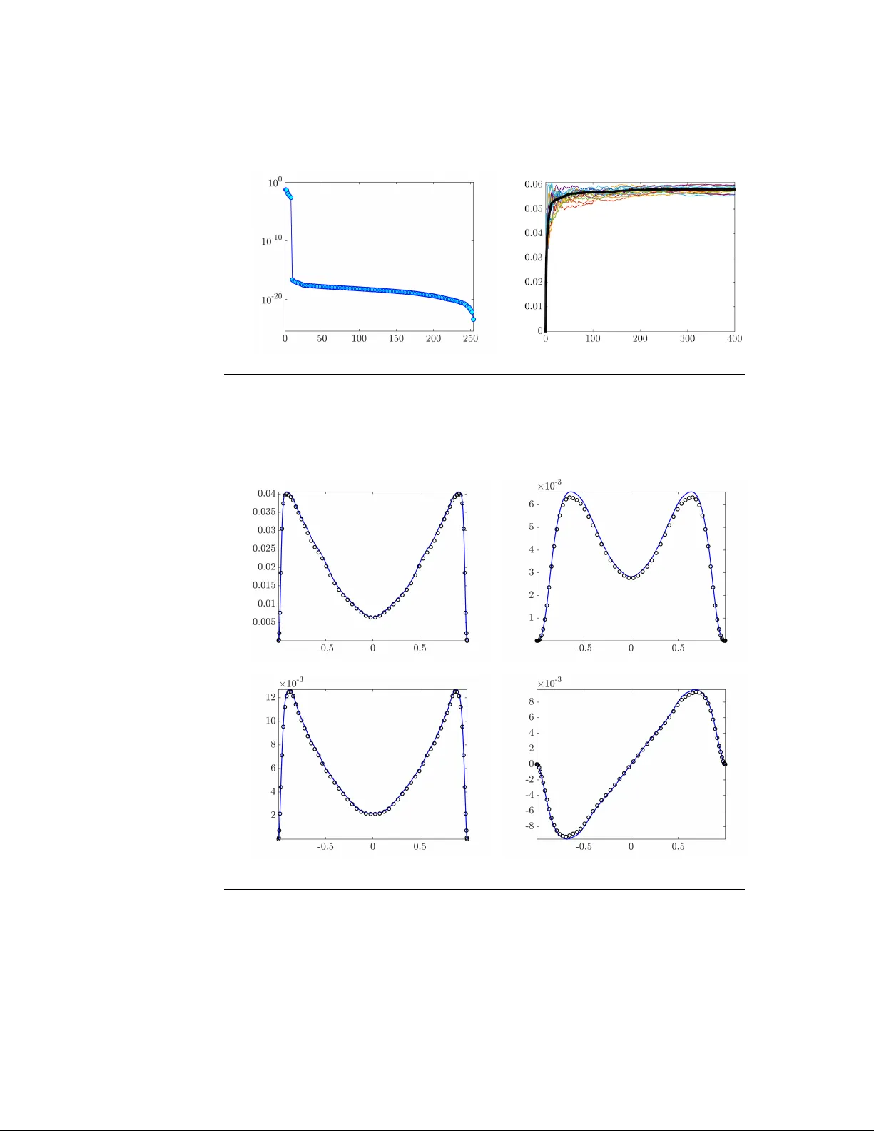
Sto c hastic dynamical mo deling of turbulen t flo ws A. Zare 1 , T. T. Georgiou 2 , and M. R. Jo v ano vi´ c 3 1 Department of Mechanical Engineering, Universit y of T exas at Dallas, Richardson, T exas 75080, USA 2 Department of Mechanical and Aerospace Engineering, Universit y of California, Irvine, California 92697, USA 3 Ming Hsieh Department of Electrical and Computer Engineering, University of Southern California, Los Angeles, California 90089, USA; email: mihailo@usc.edu Annu. Rev. Control Rob ot. Auton. Syst. 2019. 3:1–26 https://doi.org/10.1146/((please add article doi)) Copyrigh t © 2019 by Annual Reviews. All rights reserved Keyw ords flo w modeling and control, con trol theory , con vex optimization, data-driv en con trol-oriented mo deling, Na vier-Stokes equations, sto c hastic dynamics, turbulent flo ws Abstract Adv anced measuremen t tec hniques and high p erformance computing ha ve made large data sets a v ailable for a wide range of turbulent flows that arise in engineering applications. Dra wing on this abundance of data, dynamical models can be constructed to reproduce structural and statistical features of turbulent flo ws, op ening the wa y to the design of effectiv e mo del-based flo w control strategies. This review describ es a framew ork for completing second-order statistics of turbulen t flo ws b y mo dels that are based on the Navier-Stok es equations linearized around the turbulen t mean velocity . Systems theory and con vex optimization are combined to address the inherent uncertaint y in the dynamics and the statistics of the flo w b y seeking a suitable parsimonious correction to the prior linearized mo del. Sp ecifically , dynamical couplings b e- t ween states of the linearized mo del dictate structural constrain ts on the statistics of flow fluctuations. Thence, colored-in-time stochastic forcing that drives the linearized mo del is sough t to account for and reconcile dynamics with a v ailable data (i.e., partially known second order statistics). The num b er of dynamical degrees of freedom that are directly affected b y sto c hastic excitation is minimized as a measure of mo del parsimony . The sp ectral conten t of the resulting colored-in- time sto chastic contribution can alternatively b e seen to arise from a lo w-rank structural p erturbation of the linearized dynamical generator, p oin ting to suitable dynamical corrections that may accoun t for the absence of the nonlinear in teractions in the linearized mo del. 1 1. INTRODUCTION T urbulent flows are at the cen ter of man y key pro cesses in nature and in engineering appli- cations. Energy dissipation caused by turbulent fluctuations around airplanes, ships, and submarines increases resistance to motion (i.e., skin-friction drag) and fuel consumption and compromises the performance of vehicles. This motiv ates the design of flo w con trol strategies for the improv ed p erformance of air and water vehicles and other systems that in volv e turbulen t flo ws (1, 2). Mo dels that are based on the Navier-Stok es (NS) equations capture the dynamics and statistical features of fluid flows. How ever, these mo dels are giv en by 3D nonlinear PDEs and they inv olv e a num b er of degrees of freedom that is prohibitively large for analysis and con trol synthesis (3, 4). Moreo ver, to this da y , a detailed understanding of the mechanisms resp onsible for the dissipation of energy in turbulent flo ws is missing. As a result, traditional flo w control techniques are largely empirical, and they rely on physical intuition, numerical sim ulations, and exp erimen ts. Ev en though these pro vide in v aluable insights, they are costly , time-consuming, and are not suitable for mo del-based con troller design. Direct numerical sim ulation (DNS) offers a computational approach to finding a solution to the NS equations. At moderate Reynolds n umbers DNS provides important insigh t into structural and statistical features of turbulen t flo ws but computational complexit y increases roughly as the cub e of the Reynolds n umber and DNS b ecomes prohibitively expensive in most flow regimes that are encountered in engineering practice (3). An alternative to DNS has b een to either fully resolve large-scale 3D turbulen t flo w structures and to mo del the impact of smaller scales or to focus on statistical signatures of turbulent flo ws, i.e., the mean flo w components and their higher-order moments. The former approach gives rise to large-eddy simulation (LES) which relies on mo deling the impact of small unresolv ed ph ysical scales (5), and the latter forms the basis for statistical theory of turbulence (6). While LES accurately captures large-scale unsteady motions that dominate flows around air and water vehicles, its computational cost is still to o high for it to b e incorp orated in to aero dynamic design (4). Since an exact set of dynamical equations that go v ern the ev olution of statistics of turbulent flows do es not exist, the statistical theory of turbulence aims to dev elop appro ximate mathematical mo dels for turbulent flo ws (7). Indeed, recen t research suggests that conv entional techniques can b e significantly enhanced using low-complexit y mo dels that are conv enient for real-time control design and optimization (8). In general, mo deling can be seen as an inv erse problem where a searc h in parameter space aims to identify a parsimonious representation of data. F or turbulent flows, the adv ent of adv anced measurement techniques and high performance parallel computing has resulted in large data sets for a wide range of flo w configurations and speeds. T apping on this abundance of data, dynamical mo dels can b e constructed to repro duce structural and statistical features of turbulent flo ws. The prev alence of coherent structures in turbulen t w all-b ounded shear flo ws (9, 10, 11, 12) has inspired the developmen t of data-driven techniques for reduced-order modeling of turbulent flows (13, 14, 15, 16, 17, 18). Ho wev er, unreliable measurements and data anomalies challenge a sole reliance on data as such mo dels are agnostic to the underlying ph ysics. F urthermore, control actuation and sensing may significantly alter the iden tified mo des in unpredictable w ays. This compromises the p erformance of data-driv en mo dels in regimes that w ere not accounted for in the training pro cess and in tro duces nontrivial c hallenges for mo del-based con trol design (19, 20). A promising alternativ e is to lev erage the underlying ph ysics in the form of a prior mo del that arises from first principles, e.g., 2 Zar e, Ge or giou, Jovanovi´ c linearization of the NS equations around stable flow states. The sub ject of this review is to highlight recent dev elopments in combining data-driv en techniques with systems theory and optimization to enhance predictiv e capabilities of ph ysics-based dynamical models. Ov er the last three decades, important dynamical asp ects of transitional and turbulent flo ws hav e b een captured by the analysis of the linearized NS equations. Sp ecifically , the non-normalit y of the linearized dynamical generator introduces in teractions among expo- nen tially deca ying normal mo des (21, 22). This property has b een used to explain high flo w sensitivit y in the early stages of transition and to iden tify key mec hanisms for sub- critical transition to turbulence; even in the absence of modal instability , bypass routes to transition can b e triggered by large transient growth (23, 24, 25, 26, 27) or large am- plification of deterministic and sto chastic disturbances (21, 28, 29, 30, 31, 32). Similar amplification mechanisms hav e b een observ ed for the linearized NS equations around the turbulen t mean v elo city (30, 33, 34, 35, 36). Additional insigh ts in to the geometric scaling of dominant modes o ver v arious flow conditions hav e b een provided by low-order represen- tations resulting from singular v alue decomposition of the asso ciated frequency response op erator (36, 37, 38). The nonlinear terms in the NS equations play an imp ortant role in the growth of flow fluctuations, transition to turbulence, and in sustaining turbulent flo w. Since these terms are conserv ative, they do not contribute to the transfer of energy b etw een the mean flow and velocity fluctuations, but they transfer energy b etw een different spatio-temporal F ourier mo des (39, 7). This feature has inspired modeling the effect of nonlinearit y using additive forcing to the linearized equations that gov ern the dynamics of fluctuations. Early efforts in this direction focused on mo deling homogeneous isotropic turbulence (40, 41, 42, 43). Sto c hastically-forced linearized NS equations were later used to model heat and momentum fluxes as well as spatio-temp oral sp ectra in quasi-geostrophic turbulence (44, 45, 46), while structural features of w all-b ounded turbulen t flo ws w ere captured using the spatio-temporal frequency responses of the linearized NS equations (28, 29, 30, 31, 36, 47, 48, 49). In these studies, forcing is used to mo del exogenous excitation sources and uncertain initial conditions, as well as to replicate the effects of the nonlinear terms in the full NS equations. This review explains how sto chastic dynamical mo dels can enhance the linearized NS equations so as to accurately replicate observed statistical features of turbulent flo ws. This is accomplished by bringing together to ols from systems theory and conv ex optimization in order to suitably shap e the p ow er sp ectrum of additiv e stochastic forcing in to the dynamical equations. W e focus on replicating second-order statistics and cast the corresp onding model iden tification as a conv ex optimization problem. The resulting sto chastic comp onent can b e linked to a structural (low-rank) perturbation of the dynamical generator suggesting suitable correction to account for the absence of the nonlinear interactions. The review is organized as follows. In Section 2, w e pro vide the bac kground on the NS equations and turbulence mo deling. In Section 3, we introduce the stochastically-forced linearized NS equations and describ e structural constraints on admissible state cov ariances and input pow er sp ectra. In Section 4, w e demonstrate the necessit y for colored-in-time sto c hastic forcing and formulate a con vex optimization problem aimed at matc hing a v ailable and completing unav ailable second-order statistics of turbulent flo ws via low-complexit y sto c hastic dynamical mo dels. In Section 5, we apply the stochastic mo deling approac h of Section 4 to a turbulent c hannel flo w, verify its utility in linear sto chastic simulations, and examine the resulting spatio-temp oral sp ectrum. W e close the pap er by discussing the outstanding research issues and pro vide concluding remarks in Section 6. www.annualr eviews.org • Sto chastic dynamic al modeling of turbulent flows 3 2. THE NA VIER-STOKES EQUA TIONS Flo ws of incompressible Newtonian fluids are gov erned by the NS and con tinuit y equations, ∂ t u + ( u · ∇ ) u = −∇ P + 1 Re ∆ u , 0 = ∇ · u , (1) where u is the velocity vector whic h satisfies the no-slip and no-p enetration b oundary conditions at a stationary solid surface, P is the pressure, ∇ and ∆ = ∇ · ∇ are the gradien t and Laplacian operators, and ∂ t is the partial deriv ativ e with resp ect to time. The NS equations are nonlinear PDEs in spatial co ordinates x and time t and the contin uity equation reflects the static-in-time div ergence-free requirement on the velocity field. The flo w is parameterized b y the Reynolds num b er whic h determines the ratio of inertial to viscous forces, R e : = ¯ uh/ν , where ¯ u and h are the characteristic v elo city and length of the flow and ν is the kinematic viscosit y . Spatial co ordinates in Equation 1 are non-dimensionalized by h , velocity by ¯ u , time b y h/ ¯ u , and pressure by ρ ¯ u 2 , where ρ is the fluid density . Mean flo w equations and the closure problem When the flo w becomes turbulent, it reaches a statistically stationary state in whic h v ari- ables still v ary in time but their statistics are time-indep endent. T o analyze the statistical prop erties of the flo w, the velocity and pressure fields are decomposed into the sum of the turbulen t mean comp onents ( ¯ u , ¯ P ) and fluctuations ( v , p ) around them, ( u , P ) = ( ¯ u + v , ¯ P + p ) , ( ¯ u , ¯ P ) = ( h u i , h P i ) , ( h v i , h p i ) = (0 , 0) , where h·i denotes the time-a verage op erator, e.g., h u ( x , t ) i = lim T → ∞ 1 T Z T 0 u ( x , t + τ ) d τ . Av eraging Equation 1 yields the Reynolds-av eraged NS equations (39, 50, 51), ∂ t ¯ u + ( ¯ u · ∇ ) ¯ u = −∇ ¯ P + 1 Re ∆ ¯ u − ∇ ·  vv T  , 0 = ∇ · ¯ u , (2) whic h gov ern the evolution of the turbulent mean profiles ( ¯ u , ¯ P ). Relative to the NS equa- tions 1, the mean-momentum equations 2 contain one additional term which dep ends on the second order moment of the velocity fluctuation vector v ,  vv T  . This symmetric tensor arises from momentum transfer b y the velocity fluctuations and it has profound influence on the mean flo w quantities and thereb y on our abilit y to predict the skin-friction drag (39). F or a three-dimensional flow, Equation 2 consists of four indep endent equations go vern- ing the dynamics of the mean velocity and pressure fields ( ¯ u , ¯ P ). How ever, these equations con tain more than four unknowns; in addition to ¯ u and ¯ P , the R eynolds str esses  vv T  are also unknown. This is a consequence of a closur e pr oblem that cannot b e resolved in the absence of additional information ab out the second-order statistics of velocity fluctuations. Since the NS equations are nonlinear, the n th velocity moment depends on the ( n + 1)th momen t (39) making it c hallenging to determine such second-order statistics. Statistical theories of turbulence attempt to ov ercome the closure problem by mo deling the effect of the Reynolds stress tensor on the mean flow quan tities rather than explic- itly resolving the nonlinear terms (39, 50, 51). This is typically ac hieved by expressing 4 Zar e, Ge or giou, Jovanovi´ c mean flo w equations turbulence model turbulent mean v elo city second-order statistics (a) mean flo w equations linearized dynamics stochastic forcing turbulent mean v elo city second-order statistics (b) Figure 1 (a) Con ven tional turbulence mo dels are used to compute second-order statistics whic h drive the mean flow equations. (b) An alternativ e approac h utilizes sto chastically-forced linearized dynamics around the turbulent mean velocity to compute the second-order statistics of velocity fluctuations. higher-order moments in terms of the low er-order moments via a com bination of physical in tuition and empirical observ ations with rigorous approximation of the flow equations; see Figure 1(a) . F or example, the turbulent viscosity hypothesis seeks appro ximate solutions of Equation 2 by relating turbulent stresses to mean velocity gradients via (51), D vv T E − 1 3 trace D vv T E I = − ν T Re  ∇ ¯ u + ( ∇ ¯ u ) T  , where ν T is the turbulent viscosity and I is the identit y tensor. Unfortunately , a general purp ose expression for ν T do es not exist and turbulence models are required to relate it to other flow quantities, e.g., second-order statistics of the v elo city fluctuations. With appropriate choices of velocity and length scales, turbulen t viscosity can b e ex- pressed as (51) ν T = cRe 2 ( k 2 / ) , where k and  denote the turbulen t kinetic energy and its rate of dissipation and c is the constan t. The k -  model (52, 53) pro vides tw o differen tial transport equations for comput- ing k and  and it is widely used in commercial computational fluid dynamics co des and in engineering practice. Even though these are less complex than the NS equations, they are still computationally exp ensive, pro duce reliable result only for certain flo w configura- tions, and are not con venien t for control design and optimization; see (51) for additional details. In what follo ws, w e describ e an alternative approach to turbulence modeling, which appro ximates the Reynolds stresses using the second-order statistics of the sto chastically- forced NS equations linearized around the turbulent mean flow; see Figure 1(b) . W e also demonstrate ho w second-order statistics resulting from DNS and experiments can b e used to refine the predictive capabilit y of mo dels that arise from first principles. www.annualr eviews.org • Sto chastic dynamic al modeling of turbulent flows 5 (a) (b) y U ( y ) Figure 2 (a) Geometry of a pressure-driven turbulent c hannel flo w b etw een tw o parallel infinite walls. (b) T urbulent mean v elocity profile U ( y ) in a flo w with friction Reynolds n umber Re = 186. 3. STOCHASTICALL Y-FORCED LINEARIZED NA VIER-STOKES EQUA TIONS The dynamics of small velocity and pressure fluctuations ( v , p ) around the turbulent mean profile ( ¯ u , ¯ P ) are go verned by the linearized NS and contin uity equations ∂ t v + ( ∇ · ¯ u ) v + ( ∇ · v ) ¯ u = −∇ p + 1 Re ∆ v + d , (3a) 0 = ∇ · v . (3b) Here, d represents an additive zero-mean stationary sto chastic input that triggers a sta- tistical resp onse of the linearized dynamics. In what follows, we describe how a v ailable second-order statistics of turbulent channel flows can be reproduced using the sto chastically- forced mo del represented b y Equation 3 and a suitable choice of p ow er sp ectrum for the input d . While w e fo cus on the turbulent channel flow, it is noteworth y that the reviewed metho dology and theoretical framework are applicable to other flo w configurations. In strongly inertial regimes, all flows transition to turbulence and a c hannel flo w, with geometry shown in Figure 2(a) , is commonly used as a benchmark for mo deling, analysis, and con trol of wall-bounded turbulence. As illustrated in Figure 2(b) , the turbulen t mean v elo city in channel flow only contains a streamwise comp onent ¯ u = [ U ( y ) 0 0 ] T , and the linearized model that go v erns the dynamics of velocity fluctuations v : = [ u v w ] T , in the stream wise, x , wall-normal, y , and span wise, z , directions tak es the form, ∂ t u + U ( y ) ∂ x u + U 0 ( y ) v = − ∂ x p + (1 /Re ) ∆ u + d u ∂ t v + U ( y ) ∂ x v = − ∂ y p + (1 /Re ) ∆ v + d v ∂ t w + U ( y ) ∂ x w = − ∂ z p + (1 /Re ) ∆ w + d w 0 = ∂ x u + ∂ y v + ∂ z w. (4) Here, U 0 ( y ) : = d U ( y ) / d y and d : = [ d u d v d w ] T is the bo dy forcing fluctuation vector. By selecting the channel half-heigh t h and the friction velocity u τ as the prop er scales, the flow is characterized by the friction Reynolds num b er Re : = u τ h/ν . The linearized dynamics in Equation 4 are time-inv ariant and hav e constant co efficients in the wall-parallel directions; thus, the F ourier transform in x and z can be used to obtain a 6 Zar e, Ge or giou, Jovanovi´ c one-dimensional system of PDEs (in y and t ) parameterized by the horizon tal wa ven umbers k : = ( k x , k z ). F urthermore, a standard con version can b e used to eliminate the pressure from the equations and bring the descriptor form in Equation 4 in to the form of an evolution mo del in which the state is determined by the wall-normal velocity , v , and vorticit y , η = ∂ z u − ∂ x w , fluctuations (54, 31) with the b oundary conditions v ( y = ± 1 , k , t ) = ∂ y v ( y = ± 1 , k , t ) = η ( y = ± 1 , k , t ) = 0. A pseudo-spectral technique (55) with N collocation p oints in y approximates the underlying operators and a change of v ariables describ ed in (56, App endix A) is used to obtain a finite-dimensional state-space representation in which the energy of velocity fluctuations at an y k is determined by the Euclidean norm of the state v ector ψ : = [ v η ] T , ˙ ψ ( k , t ) = A ( k ) ψ ( k , t ) + B ( k ) d ( k , t ) , v ( k , t ) = C ( k ) ψ ( k , t ) . (5) Here, ψ ( k , t ) ∈ C 2 N , d ( k , t ) ∈ C 3 N is the input vector, v ( k , t ) ∈ C 3 N is the v elocity fluctuation vector, the matrix A ( k ) determines dynamical interactions b etw een the state v ariables, B ( k ) sp ecifies the wa y the input d ( k , t ) en ters in to the evolution model, and the output matrix C ( k ) relates the state v ector ψ ( k , t ) to the v elo city fluctuation vector v ( k , t ). The ev olution model is obtained from Equation 4 as follows. Applying the div ergence operator ∇ to the linearized NS equations yields an expression for ∆ p . The equation for v is obtained b y acting with the Laplacian ∆ on the second equation in Model 4 and utilizing the expression for ∆ p to eliminate the pressure p . The equation for η is obtained b y taking the curl of the linearized NS equations. This yields t wo PDEs that go vern the evolution of v and η that in volv e only v , η , and d . The linearized NS equations around the turbulen t mean velocity profile are stable (57, 58), i.e., all eigen v alues of A in Equation 5 are in the left-half of the complex plane. 3.1. Algebraic relations b etw een input and state statistics In channel flow, the NS equations linearized around the turbulent mean flo w are stable (57, 58) and the steady-state co v ariance matrix X ( k ) of the state v ector in Equation 5 X ( k ) = lim t → ∞ E ( ψ ( k , t ) ψ ∗ ( k , t )) , (6) satisfies the Ly apunov-lik e equation (59, 60) A ( k ) X ( k ) + X ( k ) A ∗ ( k ) = − B ( k ) H ∗ ( k ) − H ( k ) B ∗ ( k ) , (7) where E is the expectation operator and ∗ is complex-conjugate-transp ose. F or colored-in- time d ( k , t ), H ( k ) is a matrix that quantifies the cross-correlation betw een the input and the state in Equation 5 in statistical steady-state (56, Appendix B), H ( k ) = lim t → ∞ E ( ψ ( k , t ) d ∗ ( k , t )) + 1 2 B ( k ) Ω( k ) . When the input d ( k , t ) in Equation 5 is zero-mean and white-in-time with co v ariance matrix Ω( k ), i.e., E ( d ( k , t )) = 0 and E ( d ( k , t ) d ∗ ( k , τ )) = Ω( k ) δ ( t − τ ), H ( k ) simplifies to H ( k ) = (1 / 2) B ( k )Ω( k ) and Equation 7 reduces to the standard algebraic Lyapuno v equation, A ( k ) X ( k ) + X ( k ) A ∗ ( k ) = − B ( k ) Ω( k ) B ∗ ( k ) . (8) The steady-state v elo city co v ariance matrix V ( k ) can be obtained from X ( k ), V ( k ) = lim t → ∞ E ( v ( k , t ) v ∗ ( k , t )) = C ( k ) X ( k ) C ∗ ( k ) . (9) Since the dynamics are parameterized b y w av enum b ers k , the en tries of V ( k ) determine t wo-point correlations of v elo city fluctuations in the wall-normal direction y ; see (61). www.annualr eviews.org • Sto chastic dynamic al modeling of turbulent flows 7 3.2. Spatio-temp oral correlations A t any k , the matrix V ( k ) determines tw o-p oint correlations in the w all-normal direction of velocity fluctuations in statistical steady-state and the lagged co v ariance matrix, R vv ( k , τ ) : = lim t → ∞ E ( v ( k , t ) v ∗ ( k , t + τ )) , (10) captures spatio-temp oral correlations. F urthemore, the application of the temp oral F ourier transform yields the sp ectral densit y matrix S vv ( k , ω ) of the output v ( k , t ), S vv ( k , ω ) = Z + ∞ −∞ R vv ( k , τ ) e − i ωτ d τ , (11) whic h parameterizes t w o-p oint velocity correlations across wa ven umbers k and temp oral frequencies ω . The matrix S vv ( k , ω ) can b e expressed in terms of the spectral density matrix S dd ( k , ω ) of the input d ( k , t ), S vv ( k , ω ) = T vd ( k , ω ) S dd ( k , ω ) T ∗ vd ( k , ω ) , where T vd ( k , ω ) is the spatio-temp oral frequency response of the L TI system in Equation 5, v ( k , ω ) = T vd ( k , ω ) d ( k , ω ) = C ( k ) (i ω I − A ( k )) − 1 B ( k ) d ( k , ω ) . (12) The steady-state output cov ariance matrix V ( k ) is related to the sp ectral density matrix S vv ( k , ω ) via, V ( k ) : = R vv ( k , 0) = 1 2 π Z + ∞ −∞ S vv ( k , ω ) d ω . (13) Finally , for white-in-time input d ( k , t ) in Equation 5, the lagged output cov ariance matrix R vv ( k , τ ) can b e expressed as a linear function of the steady-state cov ariance matrix X ( k ), R vv ( k , τ ) = C ( k ) X ( k ) e A ∗ ( k ) τ C ∗ ( k ) . (14) Summa ry F or the L TI dynamics in Equation 5, the algebraic constrain t in Equation 7 determines admissible steady-state cov ariance matrices X ( k ). Among all p ositive semi- definite matrices, this constrain t iden tifies those that qualify as state-co v ariances for a state- space represen tation with matrices A ( k ) and B ( k ). As sho wn in (59, 60), the structure of state-co v ariances is an inheren t property of the linear dynamics. The sidebar ADMISSIBLE CO V ARIANCES describ es necessary and sufficien t conditions for a p ositive-definite matrix X ( k ) to qualify as a steady co v ariance matrix of the state ψ ( k , t ) in Equation 5. These conditions amount to the solv abilit y of Equation 15b for the matrix H ( k ) or, equiv alently , the rank condition in Equation 15a. W e next build on such structural constraints on admissible cov ariances and formulate con v ex optimization problems for characterizing the statistical properties of stochastic excitations to L TI systems that account for partially a v ailable statistics in turbulen t channel flow. 4. COMPLETION OF P ARTIALL Y A V AILABLE FLOW ST A TISTICS The algebraic relations describ ed in Section 3.1 can b e used to compute the steady co- v ariance matrix X ( k ) of the sto chastically-forced L TI system in Equation 5 based on the 8 Zar e, Ge or giou, Jovanovi´ c ADMISSIBLE CO V ARIANCES The matrix X = X ∗  0 is the stationary co v ariance matrix of the state of the L TI system in Equation 5 with controllable pair ( A, B ) and suitable input pro cess d if and only if rank " AX + X A ∗ B B ∗ 0 # = rank " 0 B B ∗ 0 # , (15a) or equiv alently , if and only if the matrix equation B H ∗ + H B ∗ = − ( A X + X A ∗ ) , (15b) has a solution H (59, 60). The rank condition in Equation 15a implies that any p ositive-definite matrix X is admissible as a stationary cov ariance of the state of an L TI system if the input matrix B is full row rank. linearized model (i.e., the matrices A ( k ) and B ( k )) and the input statistics. In stochastic dynamic mo deling of turbulent flows, how ev er, the conv erse question is of interest: starting from the co v ariance matrix X ( k ) and the dynamic matrix A ( k ) in Equation 5, the ob jec- tiv e is to identify the directionality of the disturbance (i.e., the matrix B ( k ) in Equation 5) and the pow er spectrum of the sto chastic input d ( k , t ) that generate such state statistics. As illustrated in Figure 3(a) , this amounts to designing a linear filter which is driven by white noise and produces input d ( k , t ) that generates the desired cov ariance matrix X ( k ) for the L TI system in Equation 5. In high-Reynolds-n umber flo ws, experimental and com- putational limitations often lead to only partial knowledge of flow statistics. F or example, in exp eriments, an arra y of probes may only provide a limited subset of spatio-temp oral correlations for velocity fluctuations, and in numerical simulations, certain regions of the computational domain may be po orly resolved. In this section, we form ulate the prob- lem of completing partially known state correlations in a wa y that is consistent with the h yp othesis that perturbations around the turbulent mean v elo city are generated by the linearized NS equations. T o accomplish this ob jective, we seek sto chastic forcing models of lo w-complexity where complexity is quantified by the num b er of degrees of freedom that are directly influenced by sto c hastic forcing in the linearized evolution mo del. 4.1. Necessity for colored-in-time sto chastic forcing The right-hand-side of standard algebraic Ly apuno v equation 8 is sign-definite, i.e., B ( k ) Ω( k ) B ∗ ( k )  0. In contrast, the righ t-hand-side of Ly apunov-lik e equation 7 is in general sign-indefinite and, unless the input d ( k , t ) in Equation 5 is white-in-time, matrix Z ( k ) : = − ( A ( k ) X ( k ) + X ( k ) A ∗ ( k )) = B ( k ) H ∗ ( k ) + H ( k ) B ∗ ( k ) , (16) can hav e both positive and negativ e eigen v alues. Figure 4 sho ws the eigen v alues of the matrix A ( k ) X dns ( k ) + X dns ( k ) A ∗ ( k ) for a c hannel flo w with R e = 186 and k = (2 . 5 , 7), where A ( k ) denotes the generator of the dynamics in Equation 5 obtained by linearization around the turbulen t mean velocity profile and X dns ( k ) is the steady-state co v ariance ma- trix resulting from numerical sim ulations of the nonlinear NS equations. The presence of www.annualr eviews.org • Sto chastic dynamic al modeling of turbulent flows 9 filter linearized dynamics white noise w velocity fluctuations v colored noise d (a) modified dynamics white noise w velocity fluctuations v (b) Figure 3 (a) The cascade connection of the linearized dynamics with a spatio-temporal linear filter whic h is designed to account for partially a v ailable second-order statistics of turbulent channel flow; (b) An equiv alent reduced-order representation of the cascade connection in (a). λ i ( A X dns + X dns A ∗ ) i Figure 4 Positiv e eigenv alues of the matrix A ( k ) X dns ( k ) + X dns ( k ) A ∗ ( k ) for c hannel flo w with Re = 186 and k = (2 . 5 , 7), indicate that turbulent v elocity co v ariances cannot b e reproduced by the linearized NS equations with white-in-time sto chastic forcing (cf. Equation 8). b oth p ositive and negative eigen v alues indicates that the second-order statistics of turbu- len t channel flow cannot b e reproduced by the linearized NS equations with white-in-time sto c hastic excitation. The mo deling and optimization framew ork that w as recently dev el- op ed in (62, 56) ov ercomes this limitation by departing from the white-in-time restriction on sto chastic forcing. 4.2. Covariance completion via convex optimization F or the dynamical generator A resulting from linearization of the NS equations around the turbulen t mean velocity , the steady-state co v ariance matrix X satisfies A X + X A ∗ + Z = 0 , (17a) where Z : = B H ∗ + H B ∗ , (17b) quan tifies the contribution of stochastic excitation. F or notational con venience, w e omit the dep endence on the wa ven um b er k in this section. W e assume that a subset of entries of 10 Zar e, Ge or giou, Jovanovi´ c V uv V uw V vv V vw V ww V uu Figure 5 Structure of the output cov ariance matrix V . Av ailable one-p oint correlations of the velocity vector v in the wall-normal direction at v arious w av enumbers k are marked b y the orange lines. the output cov ariance matrix V , namely V ij for a selection of indices ( i, j ) ∈ I , is av ailable. This yields an additional set of linear constrain ts for the matrix X , ( C X C ∗ ) ij = V ij , ( i, j ) ∈ I . (17c) F or example, suc h kno wn entries ma y represen t one-point correlations in the w all-normal di- rection; see Figure 5 for an illustration. At an y k , the diagonals of the submatrices V uu ( k ), V vv ( k ), and V ww ( k ) denote the normal Reynolds stresses in turbulen t channel flow, e.g., diag ( V uu ( k )) = diag  lim t → ∞ E ( u ( k , t ) u ∗ ( k , t ))  , and the main diagonal of the submatrices V uv ( k ), V uw ( k ), and V vw ( k ) denote the shear stresses, e.g., diag ( V uv ( k )) = diag (lim t → ∞ E ( u ( k , t ) v ∗ ( k , t ))) . It is noteworth y that while the co v ariance matrix X is not allo wed to hav e negative eigen v alues, the matrix Z can b e sign indefinite. Our ob jective is to identify suitable choices of X and Z that satisfy the ab o ve constrain ts and yield a lo w-complexity model for the sto chastic input that explains the observed statistics. In statistical steady-state, turbulent kinetic energy is determined by the sum of traces of matrices V uu , V vv , and V ww and skin-friction drag depends on the shear stress diag ( V uv ). The con tribution of the sto chastic excitation en ters through the matrix Z , whic h is of the form given by Equation 17b, where the directionality of the input and its time-correlations are reflected b y the c hoices of matrices B and H . As discussed in the sidebar ADMISSIBLE CO V ARIANCES, when the input matrix B is full rank an y positive semi-definite X qualifies as the steady-state cov ariance of sto chastically-forced linearized NS equations 5. Ho wev er, as demonstrated in (56), in this case a forcing mo del that cancels the linearized dynamics and obscures important asp ects of the underlying ph ysics becomes a viable option. It is th us imp ortan t to minimize the num b er of degrees of freedom that can be directly influenced by sto c hastic forcing. This can b e accomplished via suitable regularization, e.g., by minimizing rank of the matrix Z in Equation 17a (63, 62). The rank of the matrix Z bounds the num b er of independent input channels or columns in matrix B ; see (62) for details. This giv es rise to the conv ex optimization problem CC-1 describ ed in the sidebar CO- V ARIANCE COMPLETION PROBLEM. The ob jective function in CC-1 pro vides a trade- off b etw een the solution to the maximum entrop y problem and the complexity of the forc- ing mo del, where the p ositive regularization parameter γ reflects the relativ e weigh t of the n uclear norm ob jective. The conv exity of optimization problem CC-1 follows from the con- v exity of the ob jective function and the linearit y of the constraint set, thereby implying the existence of a globally optimal minimizer. www.annualr eviews.org • Sto chastic dynamic al modeling of turbulent flows 11 CO V ARIANCE COMPLETION PROBLEM Giv en matrices A and C , the a v ailable en tries V ij of the output cov ariance matrix V , and p ositive regular- ization parameter γ , determine the Hermitian matrices X and Z that solv e conv ex optimization problem minimize X, Z − log det ( X ) + γ k Z k ? sub ject to A X + X A ∗ + Z = 0 ( C X C ∗ ) ij = V ij , ( i, j ) ∈ I . (CC-1) The first constrain t reflects the requirement that the second-order statistics are consisten t with sto c hastically-forced linearized mo del and the second constraint requires that the a v ailable elemen ts of the matrix V are exactly repro duced. Minimizing the logarithmic barrier function ensures positive-definiteness of the cov ariance matrix X (64) and results in a maximum entrop y stochastic realization (65). On the other hand, the nuclear norm regularizer, i.e., the sum of singular v alues of the matrix Z , k Z k ? = P i σ i ( Z ), is in tro duced to restrict the rank of Z (66, 67) and thereb y reduce the complexity of the forcing mo del. 4.2.1. Po wer spectrum of stochastic input and filter design. The solution of problem CC- 1, i.e., the Hermitian matrices X ( k ) and Z ( k ), can be used to obtain a dynamical model for colored-in-time sto chastic input to the linearized NS equations. A class of generically minimal linear filters, which ha ve the same num ber of degrees of freedom as the finite- dimensional approximation of the linearized mo del, w as recently developed in (62, 56). Since channel flow is translationally inv ariant in the wall-parallel dimensions, the dy- namics in Equation 5 and optimization problem CC-1 are decoupled ov er the w av enum b ers k = ( k x , k z ). At eac h k , the filter dynamics that account for X ( k ) are giv en b y ˙ φ ( k , t ) = ( A ( k ) − B ( k ) K ( k )) φ ( k , t ) + B ( k ) w ( k , t ) , d ( k , t ) = − K ( k ) φ ( k , t ) + w ( k , t ) , (18) where φ ( k , t ) is the state of the filter and w ( k , t ) is a zero-mean white-in-time sto chastic pro cess with co v ariance Ω( k ). On the other hand, K ( k ) = ( 1 2 Ω( k ) B ∗ ( k ) − H ∗ ( k )) X − 1 ( k ) , (19) for matrices B ( k ) and H ( k ) that corresp ond to the factorization Z ( k ) = B ( k ) H ∗ ( k ) + H ( k ) B ∗ ( k ); see (62) for details. The linear filter represen ted b y Equation 18 generates a c olor e d-in-time sto chastic input d ( k , t ) to the linearized NS equations 5 and the resulting cascade connection reproduces the av ailable second-order statistics of turbulen t flo w. The sp ectral density of d ( k , t ) S dd ( k , ω ) = T dw ( k , ω ) Ω( k ) T ∗ dw ( k , ω ) , determines the spectral con tent of the input to the L TI system, where T dw ( k , ω ) = K ( k ) (i ω I − A ( k ) + B ( k ) K ( k )) − 1 B ( k ) + I , is the spatio-temporal frequency resp onse of the linear filter in Equation 18. 12 Zar e, Ge or giou, Jovanovi´ c 4.2.2. Minimal realization. The state-space representation corresp onding to the cascade connection of the linear filter in Equation 18 with the linearized NS dynamics in Equation 5 is given by " ˙ ψ ( k , t ) ˙ φ ( k , t ) # = " A ( k ) − B ( k ) K ( k ) 0 A ( k ) − B ( k ) K ( k ) # " ψ ( k , t ) φ ( k , t ) # + " B ( k ) B ( k ) # w ( k , t ) v ( k , t ) = h C ( k ) 0 i " ψ ( k , t ) φ ( k , t ) # . (20) This realization has twice as man y states as the spatial discretization of the linearized NS mo del in Equation 5, but is not controllable and therefore not minimal. As sho wn in (62), remo v al of the uncontrollable states yields the minimal realization of the mapping from the input w ( k , ω ) to the output v ( k , ω ), v ( k , ω ) = T vw ( k , ω ) w ( k , ω ), T vw ( k , ω ) = C ( k ) (i ω I − A ( k ) + B ( k ) K ( k )) − 1 B ( k ) , (21) as ˙ ψ ( k , t ) = ( A ( k ) − B ( k ) K ( k )) ψ ( k , t ) + B ( k ) w ( k , t ) , v ( k , t ) = C ( k ) ψ ( k , t ) . (22) This system has the same num b er of degrees of freedom as the system in Equation 5 and the corresp onding algebraic Lyapuno v equation in conjunction with Equation 19 yield ( A ( k ) − B ( k ) K ( k )) X ( k ) + X ( k ) ( A ( k ) − B ( k ) K ( k )) ∗ + B ( k ) Ω( k ) B ∗ ( k ) = A ( k ) X ( k ) + X ( k ) A ∗ ( k ) + B ( k ) Ω( k ) B ∗ ( k ) − B ( k ) K ( k ) X ( k ) − X ( k ) K ∗ ( k ) B ∗ ( k ) = A ( k ) X ( k ) + X ( k ) A ∗ ( k ) + B ( k ) H ∗ ( k ) + H ( k ) B ∗ ( k ) = 0 . This demonstrates that the state-space realization in Equation 18 generates a sto chastic input d ( k , t ) whic h is consisten t with the steady-state co v ariance matrix X ( k ). The effect of colored-in-time excitation is equiv alent to white-in-time excitation together with a structural perturbation of the system dynamics. Remark 1 F rom Equation 19 we have H ( k ) = 1 2 B ( k )Ω( k ) − X ( k ) K ∗ ( k ) and substitution of this expr ession into Equation 7 yields the standar d algebr aic Lyapunov e quation ( A ( k ) − B ( k ) K ( k )) X ( k ) + X ( k )( A ( k ) − B ( k ) K ( k )) ∗ = − B ( k ) Ω( k ) B ∗ ( k ) . Sinc e the p air ( A ( k ) , B ( k )) is c ontr ol lable, so ar e ( A ( k ) − B ( k ) K ( k ) , B ( k )) and ( A ( k ) − B ( k ) K ( k ) , B ( k ) Ω 1 / 2 ( k )) . Stability of the mo difie d dynamic al gener ator A ( k ) − B ( k ) K ( k ) fol lows fr om p ositive semi-definiteness of B ( k ) Ω( k ) B ∗ ( k ) via standar d Lyapunov the ory. The minimal realization (given b y Equation 22) of the cascade connection described b y Equation 20 is adv antageous from a computational standpoint and it allo ws for an alternativ e interpretation of the stochastic realization of colored-in-time forcing. First, time-domain simulations require n umerical in tegration of the system in Equation 22, which has half the num b er of states as compared to the system in Equation 20, thereby offering computational speedup. On the other hand, the structure in Equation 22 suggests that the colored-in-time forcing realized by the L TI filter in Equation 18 can be equiv alently in terpreted as a dynamical modification to the linearized equations in the form of state- feedbac k in teractions. This in terpretation pro vides an alternative viewp oint that is closely related to a class sto chastic control (68, 69, 70, 71) and output cov ariance estimation (72, 73) problems; see (62, Section I I.C) for details. Based on this, w e next describe an alternative form ulation of the cov ariance completion problem as a state-feedback syn thesis that is optimal with respect to a differen t design criterion (74, 75). www.annualr eviews.org • Sto chastic dynamic al modeling of turbulent flows 13 MINIMUM ENERGY COV ARIANCE COMPLETION PROBLEM Giv en matrices A , B , C , R , Ω, the a v ailable entries V ij of the output cov ariance matrix V , and the p ositive regularization parameter γ , determine the matrices K and X that solve conv ex optimization problem minimize K, X trace ( K ∗ R K X ) + γ n X i = 1 w i k e ∗ i K k 2 sub ject to ( A − B K ) X + X ( A − B K ) ∗ + Ω = 0 ( C X C ∗ ) ij = V ij , ( i, j ) ∈ I X  0 . (CC-2) The algebraic constraint on K and X ensures closed-lo op stability (see Remark 1 ) and consistency with the state cov ariance matrix X , and the second equality constrain t requires that the av ailable elemen ts of the matrix V are exactly repro duced. The p ositive-definite matrix R sp ecifies a p enalty on the con trol input while the w eigh ted-norm regularizer promotes sparsity on the ro ws of the matrix K . Here, w i are given p ositiv e weigh ts, e i is the i th unit vector in R m , and Ω  0 is the cov ariance matrix of white noise input w . 4.3. Minimum-control-energy covariance completion problem As describ ed in (74, 75), the challenge of establishing consistency betw een statistical mea- suremen ts and a linearized model can b e alternatively cast as the problem of seeking a completion of the missing entries of a cov ariance matrix X along with a p erturbation ∆ of the system dynamics sub ject to white-in-time input w , ˙ ψ = ( A + ∆) ψ + w , v = C ψ . F or ∆ : = − B K , a cov ariance completion problem can b e form ulated as an optimal control problem aimed at designing a stabilizing state-feedback con trol law f = − K ψ ( Figure 6 ). The choice of B may incorporate added insights in to the strength and directionalit y of p ossible couplings b et ween state v ariables. While a full-rank matrix B that allo ws the p erturbation signal K ψ to manipulate all degrees of freedom can lead to the complete can- cellation of the original dynamics A , it is also imp ortant to imp ose a p enalty on the a verage quadratic size of signals K ψ . This gives rise to con vex optimization problem CC-2 de- scrib ed in the sidebar MINIMUM ENER GY CO V ARIANCE COMPLETION PROBLEM. The ob jective function in CC-2 provides a trade-off b etw een the minimum-con trol-energy problem and the num b er of feedback couplings that need to b e introduced to mo dify the dynamical generator A and ac hieve consistency with av ailable data (74, 75). Remark 2 As demonstr ate d in (76, 62, 75), c ovarianc e completion pr oblems CC-1 and CC- 2 c an b e c ast as semidefinite pr o gr ams. F or smal l- and me dium-size pr oblems, these c an b e solve d efficiently using standar d solvers (77, 78, 64). T o de al with lar ge pr oblem dimensions that arise in fluid dynamics, customize d algorithms have b e en develop e d in (62, 75). 14 Zar e, Ge or giou, Jovanovi´ c linearized dynamics − K white noise w f velocity fluctuations v ψ Figure 6 A feedbac k connection of the linearized dynamics with a static gain matrix K that is designed to account for the sampled steady-state co v ariance matrix X . 4.4. Completion of spatio-temp oral co rrelations The co v ariance matrix V ( k ) pro vides information about spatial correlations of v elo city fluc- tuations in statistical steady-state. As described in Section 3.2, the temp oral dep endence of suc h statistics is captured by the spectral density matrix S vv ( k , ω ). This matrix can b e used to provide real-time estimates of the flo w state (79), and recent efforts ha ve been directed at estimating S vv ( k , ω ) by either matching individual entries at sp ecified temp oral frequencies (80, 81, 82) or the spectral p ow er (83), trace( S vv ( k , ω )). Either w ay it should b e independently considered whether the so-constructed colored-in-time forcing mo dels pre- serv e important asp ects of the original linearized NS dynamics. F or additional discussion on parsimonious models and how these may reflect underlying ph ysics see Section 4.2. 5. CASE STUDY: TURBULENCE MODELING IN CHANNEL FLOW In this section, w e inv estigate the completion of partially known second-order statistics of a turbulent channel flow using the framework presented in Section 4.2. The mean vel o city profile and one-p oint v elo city correlations in the wall-normal direction at v arious wa ven um- b er pairs k are obtained from DNS of a turbulent channel flow with friction Reynolds n umber Re = 186 (54, 84, 85, 86); see Figures 2(b) and 5 for an illustration. W e also sho w how the mo dified dynamics of Section 4.2.1 can be used as a lo w-dimensional model that is sim ulated in time to generate velocity fluctuations whose second-order statistics are consisten t with numerical sim ulations of the nonlinear NS equations. 5.1. Reproducing available and completing unavailable second-order statistics As demonstrated in (56), optimization problem CC-1 is feasible at all wa ven umbers k . Th us, regardless of the v alue of the regularization parameter γ , all a v ailable one-p oint correlations of turbulen t c hannel flo w can be reproduced by a sto chastically-forced linearized mo del. Figure 7 displa ys p erfect matching of all one-p oint v elo city correlations that result from in tegration o ver wall-parallel w av enum b ers. Since problem CC-1 is not feasible for Z ( k )  0 at all k , this c annot be ac hieved with white-in-time sto chastic forcing. In addition to matc hing av ailable one-p oint correlations, we next demonstrate that the solution to optimization problem CC-1 also provides go o d reco very of t wo-point correlations. These are not used as problem data in CC-1 and corresp ond to off-diagonal entries in Figure 5 . The premultiplied energy spectrum in c hannel flo w with R e = 186 p eaks at k = (2 . 5 , 7); e.g., see (87, Figure 12(a)). The left column in Figure 8 displays the streamwise www.annualr eviews.org • Sto chastic dynamic al modeling of turbulent flows 15 (a) (b) y y Figure 7 (a) Correlation profiles of normal and (b) shear stresses resulting from DNS of turbulen t channel flow with Re = 186 (–) and from the solution to CC-1; diag ( V uu ) ( # ), diag ( V vv ) ( 2 ), diag ( V ww ) ( 4 ), − diag ( V uv ) ( 3 ). Profiles are in tegrated o ver the wall-parallel w a ven umbers k . (a) (b) y V uu, dns V uu (c) (d) y V uv, dns y V uv y Figure 8 Cov ariance matrices resulting from DNS of turbulent c hannel flo w with Re = 186 (left plots); and the solution to optimization problem CC-1 with γ = 300 (right plots). (a, b) Stream wise V uu and (c,d) stream wise/wall-normal V uv cov ariance matrices for k = (2 . 5 , 7). The one-p oint correlation profiles that are used as problem data in CC-1 are marked by black lines along the main diagonals. 16 Zar e, Ge or giou, Jovanovi´ c V uu and the streamwise/w all-normal V uv co v ariance matrices resulting from DNS at these flo w conditions. The righ t column in Figure 8 shows the same co v ariance matrices that are obtained from the solution to problem CC-1; see (56) for a detailed examination of w all-normal and span wise cov ariance matrices. The qualit y of reco very depends on the c hoice of the regularization parameter γ and, for γ = 300, approximately 60% of the DNS- generated co v ariance matrix V dns can be recov ered based on a relative F rob enius norm measure, k V − V dns k F / k V dns k F . Here, V = C X C ∗ represen ts the tw o-p oint correlation matrix of v elo cit y fluctuations resulting from problem CC-1. The high-quality recov ery of t wo-point correlations is attributed to the structural constrain t in Equation 17a, whic h k eeps ph ysics in the mix and enforces consistency b etw een data and the linearized NS dynamics. While the diagonal entries of V determine the kinetic energy and affect the mean momentum transfer in the turbulen t flow, the off-diagonal tw o-p oint correlations are indicators of coherent flow structures that reside at v arious locations aw ay from the w all (88, 11). 5.2. Sto chastic linear simulations Sto c hastic simulations of the mo dified L TI dynamics in Equation 22 can b e used to v er- ify the theoretical predictions resulting from the modeling and optimization framew ork of Section 4.2. F or a spatial discretization with N = 127 collo cation p oin ts in the wall- normal direction, at each wa ven um b er k , the L TI system in Equation 22 has 254 states. F or k = (2 . 5 , 7) and γ = 10 4 , the matrix Z that solves optimization problem CC-1 has 8 non-zero eigenv alues (6 p ositive and 2 negativ e); see Figure 9(a) . As shown in (62), the maxim um num b er of positive or negativ e eigenv alues of the matrix Z b ounds the num b er of inputs into the linearized NS mo del giv en by Equation 5. This implies that partially a v ailable statistics can b e repro duced with 6 colored-in-time inputs and as a result, the dynamical mo dification B K in Equation 22 is of rank 6. Prop er comparison with DNS or experiments requires ensem ble-av eraging, rather than comparison at the lev el of individual stochastic simulations. T o this end, tw ent y simula- tions with different realizations of white-in-time input w ( k , t ) in Equation 22 hav e b een conducted. The total simulation time w as 400 viscous time units. Figure 9(b) sho ws the time evolution of the energy (v ariance) of v elo city fluctuations resulting from these tw ent y sim ulations. The v ariance av eraged ov er all simulations is mark ed by the thic k black line. Ev en though the resp onses of individual sim ulations differ from each other, the a verage of t wen ty sample sets asymptotically approaches the correct v alue of turbulent kinetic energy in statistical steady-state, trace ( V ( k )). Figure 10 displays the normal and shear stress profiles resulting from DNS and from sto chastic linear simulations. The av eraged output of the t wen ty sim ulations agrees w ell with DNS results. This agreement can b e further impro ved by running additional sim ulations and by increasing the total simulation times. 5.3. Spatio-temp oral energy sp ectrum T o analyze the spatio-temp oral asp ect of dynamical mo dels resulting from the framework of Section 4.2 we examine the Po w er Sp ectral Density (PSD) and the energy sp ectrum of v elo city fluctuations. The PSD of the L TI system in Equation 22 is determined by the sum of squares of the singular v alues of the frequency response matrix in Equation 21, Π v ( k , ω ) = trace ( T vw ( k , ω ) T ∗ vw ( k , ω )) = X i σ 2 i ( T vw ( k , ω )) . www.annualr eviews.org • Sto chastic dynamic al modeling of turbulent flows 17 (a) (b) σ i ( Z ) i kinetic energy t Figure 9 (a) Singular v alues of the solution Z to CC-1 in turbulen t channel flow with Re = 186, k = (2 . 5 , 7), and N = 127 for γ = 10 4 . (b) Time evolution of fluctuation’s kinetic energy for tw ent y realizations of the sto chastic input to the resulting modified linearized dynamics in Equation 22; the energy av eraged o ver all simulations is marked b y the thick black line. (a) (b) diag ( V uu ( k )) y diag ( V vv ( k )) y (c) (d) diag ( V ww ( k )) y diag ( V uv ( k )) y Figure 10 Normal stress profiles in the (a) stream wise, (b) w all-normal, and (c) span wise directions; (d) shear stress profile resulting from DNS of turbulen t c hannel flow with Re = 186 at k = (2 . 5 , 7) (–) and stochastic linear simulations ( # ). 18 Zar e, Ge or giou, Jovanovi´ c (a) (b) Π v ( k , ω ) ω y + ω + Figure 11 (a) P ow er sp ectral density Π v ( k , ω ) resulting from DNS of turbulen t c hannel flo w with Re = 186 at k = (2 . 5 , 7) (green), the linearized NS mo del in Equation 5 (black), an eddy-viscosity-enhanced linearized model (blue), and the modified L TI dynamics in Equation 22 for γ = 300 (red). (b) Premultiplied energy sp ectrum of the modified dynamics in Equation 22 for turbulent channel flow with Re = 186 resulting from the in tegration of ω diag ( T vw ( k , ω ) T ∗ vw ( k , ω )) ov er wa ven umbers k . In tegration of Π v ( k , ω ) ov er the temp oral frequencies yields the square of the H 2 norm of the system in Equation 22 or, equiv alently , the k -parameterized energy sp ectrum (31), E ( k ) = 1 2 Z ∞ −∞ Π v ( k , ω ) d ω = 1 2 trace ( V ( k )) . F or a turbulen t c hannel flo w with Re = 186 and k = (2 . 5 , 7), Figure 11(a) compares the p o wer spectral densities of the linearized NS model given b y Equation 5, the eddy-viscosity- enhanced modification of the linearized NS equations (89, 90, 91, 92, 48), and the dynamical mo del given b y Equation 22 resulting from the framework presen ted in Section 4.2 with the result of DNS. F or the first t wo models, the input matrix B ( k ) excites all degrees of freedom in the state equation and, for the mo dified dynamics, the input matrix B ( k ) comes from the framew ork presen ted in Section 4.2 with the regularization parameter γ = 300. All three mo dels are driven b y spatially and temp orally uncorrelated inputs. The temporal frequency at which the PSD p eaks is similar for the linearized NS equa- tions and the mo dified dynamics ( ω ≈ 45) and is closer to the result of DNS ( ω ≈ 37) than the frequency asso ciated with the eddy-viscosit y-enhanced mo del ( ω ≈ 27). W e also see that b oth the eddy-viscosit y enhancement and the data-driv en lo w-rank modification atten uate the amplification of disturbances at all temp oral frequencies. The uniform damping of the PSD ensures that the H 2 norm of the system in Equation 22 matc hes the energy spectrum of the turbulent chan nel flo w; cf. red and green curv es in Figure 11(a) . F or the mo dified dynamics giv en by Equation 22, Figure 11(b) sho ws the prem ultiplied spatio-temporal energy spectrum as a function of the wall-normal coordinate and temporal frequency in inner (viscous) units, i.e., y + : = (1 + y ) Re and ω + : = ω/Re . This sp ectrum is computed b y integrating ω diag ( T vw ( k , ω ) T ∗ vw ( k , ω )) o ver k and is concen trated around y + ≈ 15 within a frequency band ω + ∈ (0 . 01 , 1), which is in agreemen t with the trends observ ed in DNS-generated energy sp ectra (82). Impro ving the accuracy in matching the temporal correlations resulting from DNS may require closer examination of the role of parameter γ or the addition of extra constrain ts in problem CC-1 and is a sub ject of ongoing researc h. www.annualr eviews.org • Sto chastic dynamic al modeling of turbulent flows 19 SUMMARY POINTS 1. Data from numerical simulations and exp eriments can b e used to refine the predic- tiv e p ow er of models that arise from first principles, e.g., the linearized NS equations. 2. White-in-time stochastic input to the linearized NS equations cannot explain second-order statistics of turbulent w all-b ounded flo ws. 3. Colored-in-time sto chastic input that excites all degrees of freedom can completely cancel the original dynamics and yield a model that do es not generalize well. 4. A suitably regularized solution to cov ariance completion problems can ensure that imp ortan t features of spatio-temporal resp onses are captured via lo w-complexity sto c hastic dynamical mo dels. 5. The effect of colored-in-time sto chastic input can b e equiv alen tly in terpreted as a structural p erturbation of the linearized dynamical generator, whic h can b e used to iden tify important state-feedback in teractions that are lost through linearization. 6. Combining to ols and ideas from systems theory and conv ex optimization can pa ve the w ay for the systematic developmen t of theory and techniques that combine data-driv en with physics-based modeling. FUTURE ISSUES 1. Mo deling of flow disturbances plays an imp ortant role in obtaining well-possed estimation gains (93, 94). Stochastic dynamical mo dels that are obtained via co v ariance completion fit nicely in to a Kalman filtering framework for turbulen t flo ws and hav e the p otential to open the do or for a successful output-feedback design at higher Reynolds num b ers than current feedbac k (95, 96, 8) and sensor- free (97, 98, 99, 100, 87) strategies allo w. The efficacy of suc h an approach and its in terplay with real-time estimation and feedbac k con trol are yet to b e examined. 2. T urbulence modeling for complex fluids and flows in complex geometries (101, 102, 103, 104, 105, 106, 107, 108) requires dealing with a large num b er of degrees of freedom. Since impro ving up on current algorithms that require O ( n 3 ) computations for a mo del with n states is c hallenging, a possible direction is to examine physical appro ximations (109, 110, 111, 112) and model reduction tec hniques (13, 15, 16, 17). 3. The regularization terms in problems CC-1 and CC-2 are used as con vex surro- gates for rank and cardinalit y . F or problems with structural constraints suc h sur- rogates do not enjoy standard probabilistic guaran tees (113), and the utility of more refined appro ximations techniques, e.g., manifold optimization (114), lo w- rank inducing norms (115, 116), and noncon vex matrix completion (117, 118, 119) in low-complexit y sto chastic dynamical modeling remains largely unexplored. 4. Higher-order turbulent flow statistics often play an important role in c haracterizing quan tities of in terest in engineering applications; e.g., fourth-order statistics are relev ant in acoustic source mo deling for high-sp eed jets (120, 121). The importance of matc hing higher-order statistics calls for a generalized theory for the sto chastic realization of state-statistics that are currently limited to second-order correlations. 5. The output of the sto chastically-forced linear mo del can be used to drive the mean flo w equations in time-dependent sto chastic simulations. It is imp ortant to identify conditions under whic h the feedbac k interconnection in Figure 1(b) con verges. 20 Zar e, Ge or giou, Jovanovi´ c 6. CONCLUDING REMARKS This review discusses a framew ork that com bines tools from systems theory and optimiza- tion to develop low-complexit y mo dels of turbulent flows that are well-suited for analysis and con trol synthesis. The goal is to embed partially known statistical signatures obtained via numerical simulation of the NS equations or exp erimental measuremen ts into first princi- ples mo dels that arise from linearization around the turbulen t mean velocity . This amoun ts to iden tifying the sp ectral conten t of stochastic excitation into the linearized equations suc h that turbulent statistics can be reproduced. The review fo cuses on the completion of second-order statistics and while the metho dology and theoretical framew ork are applicable to a wide range of scenarios, a channel flow configuration is used to solidify the discussion. On par with the dramatic upswing from the fields of mac hine learning and optimization in lev eraging big-data for mo deling, the prop osed metho dology utilizes data to refine the predictiv e capability of a dynamical mo del that arises from first principles and it offers a new p ersp ective on tac kling issues of robustness and generalizability . DISCLOSURE ST A TEMENT The authors are not aw are of any biases that migh t b e p erceived as affecting the ob jectivit y of this review. A CKNOWLEDGMENTS Financial supp ort from NSF under Aw ards CMMI 1739243 and ECCS 1809833, and AFOSR under Awards F A9550-16-1-0009 and F A9550-18-1-0422 is gratefully ac knowledged. W e thank Anubha v Dwivedi for generating DNS results reported in Section 5.3. LITERA TURE CITED 1. Joslin RD. 1998. Aircraft laminar flow con trol. A nn. Rev. Fluid Me ch. 30:1–29 2. Gad-el Hak M. 2000. Flow control: passive, active, and reactiv e flow management. New Y ork: Cambridge University Press 3. Choi H, Moin P . 2012. Grid-p oint requiremen ts for large eddy simulation: Chapman’s estimates revisited. Phys. Fluids 24:011702 4. Slotnick J, Kho dadoust A, Alonso J, Darmofal D, Gropp W, et al. 2014. CFD vision 2030 study: A path to revolutionary computational aerosciences. T e ch. Rep. CR-2014-218178, NASA 5. Sagaut P . 2006. Large eddy sim ulation for incompressible flows: an introduction. Springer Science & Business Media 6. Wilcox DC. 1998. T urbulence modeling for CFD, v ol. 2. DCW industries La Canada, CA 7. Durbin P A, Reif BAP . 2011. Statistical theory and mo deling for turbulen t flows. Wiley 8. Kim J, Bewley TR. 2007. A linear systems approach to flow control. Annu. R ev. Fluid Me ch. 39:383–417 9. Robinson SK. 1991. Coherent motions in the turbulent boundary la yer. Annu. R ev. Fluid Me ch. 23:601–639 10. Adrian RJ. 2007. Hairpin vortex organization in wall turbulence. Phys. Fluids 19:041301 11. Smits AJ, McKeon BJ, Marusic I. 2011. High-Reynolds num b er wall turbulence. Ann. R ev. Fluid Me ch. 43:353–375 12. Jim´ enez J. 2018. Coherent structures in wall-bounded turbulence. J. Fluid Me ch. 842 13. Rowley CW. 2005. Mo del reduction for fluids using balanced prop er orthogonal decomp osition. Intl J. Bifur c ation Chaos 15:997–1013 14. Lumley JL. 2007. Stochastic to ols in turbulence. Dov er Publications www.annualr eviews.org • Sto chastic dynamic al modeling of turbulent flows 21 15. Schmid PJ. 2010. Dynamic mo de decomp osition of numerical and exp erimental data. J. Fluid Me ch. 656:5–28 16. Jov anovi ´ c MR, Schmid PJ, Nic hols JW. 2014. Sparsit y-promoting dynamic mode decomp osi- tion. Phys. Fluids 26:024103 (22 pages) 17. Rowley CW, Dawson ST. 2017. Mo del reduction for flow analysis and control. Annu. R ev. Fluid Me ch. 49:387–417 18. T owne A, Schmidt OT, Colonius T. 2018. Sp ectral proper orthogonal decomp osition and its relationship to dynamic mo de decomp osition and resolv ent analysis. J. Fluid Me ch. 847:821– 867 19. Noack BR, Morzy ´ nski M, T admor G. 2011. Reduced-order mo delling for flo w control, vol. 528 of CISM Courses and L e ctur es . Springer 20. T admor G, Noack BR. 2011. Bernoulli, Bo de, and Budgie [Ask the Exp erts]. IEEE Contr. Syst. Mag. 31:18–23 21. T refethen LN, T refethen AE, Reddy SC, Driscoll T A. 1993. Hydro dynamic stability without eigenv alues. Scienc e 261:578–584 22. Schmid PJ. 2007. Nonmo dal stability theory . Annu. R ev. Fluid Me ch. 39:129–162 23. Gustavsson LH. 1991. Energy growth of three-dimensional disturbances in plane Poiseuille flow. J. Fluid Me ch. 98:149 24. Butler KM, F arrell BF. 1992. Three-dimensional optimal perturbations in viscous shear flo w. Phys. Fluids A 4:1637 25. Reddy SC, Henningson DS. 1993. Energy gro wth in viscous channel flows. J. Fluid Me ch. 252:209–238 26. Henningson DS, Reddy SC. 1994. On the role of linear mec hanisms in transition to turbulence. Phys. Fluids 6:1396–1398 27. Schmid PJ, Henningson DS. 1994. Optimal energy density growth in Hagen-Poiseuille flow. J. Fluid Me ch. 277:197–225 28. F arrell BF, Ioannou PJ. 1993. Stochastic forcing of the linearized Na vier-Stokes equations. Phys. Fluids A 5:2600–2609 29. Bamieh B, Dahleh M. 2001. Energy amplification in c hannel flo ws with stochastic excitation. Phys. Fluids 13:3258–3269 30. Jov anovi ´ c MR. 2004. Modeling, analysis, and control of spatially distributed systems. Ph.D. thesis, Univ ersity of California, Santa Barbara 31. Jov anovi ´ c MR, Bamieh B. 2005. Comp onent wise energy amplification in c hannel flows. J. Fluid Me ch. 534:145–183 32. Ran W, Zare A, Hack MJP , Jo v anovi ´ c MR. 2019. Sto chastic receptivit y analysis of boundary lay er flow. Phys. R ev. Fluids Doi:10.1103/PhysRevFluids.00.003900; also 33. Butler KM, F arrell BF. 1993. Optimal p erturbations and streak spacing in wall-bounded tur- bulent shear flow. Phys. Fluids A 5:774–777 34. F arrell BF, Ioannou PJ. 1993. Optimal excitation of three-dimensional p erturbations in viscous constant shear flow. Phys. Fluids A 5:1390–1400 35. F arrell BF, Ioannou PJ. 1998. P erturbation structure and sp ectra in turbulent channel flow. The oret. Comput. Fluid Dynamics 11:237–250 36. McKeon BJ, Sharma AS. 2010. A critical-lay er framework for turbulent pipe flow. J. Fluid Me ch. 658:336–382 37. Moarref R, Sharma AS, T ropp JA, McKeon BJ. 2013. Mo del-based scaling of the stream wise energy densit y in high-Reynolds-n umber turbulen t channels. J. Fluid Me ch. 734:275–316 38. Moarref R, Jo v anovi ´ c MR, T ropp JA, Sharma AS, McKeon BJ. 2014. A lo w-order decomp o- sition of turbulen t channel flow via resolven t analysis and conv ex optimization. Phys. Fluids 26:051701 (7 pages) 39. McComb WD. 1991. The physics of fluid turbulence. Oxford Univ ersity Press 40. Kraichnan RH. 1959. The structure of isotropic turbulence at very high Reynolds numbers. J. 22 Zar e, Ge or giou, Jovanovi´ c Fluid Me ch. 5:497–543 41. Kraichnan RH. 1971. An almost-Marko vian Galilean-inv ariant turbulence model. J. Fluid Me ch. 47:513–524 42. Orszag SA. 1970. Analytical theories of turbulence. J. Fluid Me ch. 41:363–386 43. Monin AS, Y aglom AM. 1975. Statistical fluid mec hanics, vol. 2. MIT Press 44. F arrell BF, Ioannou PJ. 1993. Stochastic dynamics of baro clinic wav es. J. Atmos. Sci. 50:4044– 4057 45. F arrell BF, Ioannou PJ. 1994. A theory for the statistical equilibrium energy sp ectrum and heat flux produced by transient baroclinic wa ves. J. Atmos. Sci. 51:2685–2698 46. DelSole T, F arrell BF. 1995. A sto chastically excited linear system as a model for quasi- geostrophic turbulence: Analytic results for one-and tw o-lay er fluids. J. Atmos. Sci. 52:2531– 2547 47. Hwang Y, Cossu C. 2010. Amplification of coheren t streaks in the turbulent Couette flo w: an input-output analysis at low Reynolds number. J. Fluid Mech. 643:333–348 48. Hwang Y, Cossu C. 2010. Linear non-normal energy amplification of harmonic and stochastic forcing in the turbulent c hannel flo w. J. Fluid Me ch. 664:51–73 49. Jov anovi ´ c MR, Bamieh B. 2001. Mo delling flow statistics using the linearized Na vier-Stokes equations. In Pr o ce e dings of the 40th IEEE Confer enc e on De cision and Contr ol 50. Durbin P A, Reif BAP . 2000. Theory and mo deling of turbulent flows. Wiley 51. Pope SB. 2000. T urbulent flows. Cam bridge Universit y Press 52. Jones W, Launder B. 1972. The prediction of laminarization with a tw o-equation mo del of turbulence. Int. J. Heat Mass T r ansf. 15:301–314 53. Launder B, Sharma B. 1974. Application of the energy-dissipation model of turbulence to the calculation of flo w near a spinning disc. L ett. He at Mass T r ansf. 1:131–137 54. Kim J, Moin P , Moser R. 1987. T urbulence statistics in fully dev elop ed channel flow at low Reynolds n umber. J. Fluid Me ch. 177:133–166 55. W eideman JA C, Reddy SC. 2000. A MA TLAB differen tiation matrix suite. A CM T r ans. Math. Softwar e 26:465–519 56. Zare A, Jo v anovi ´ c MR, Georgiou TT. 2017. Colour of turbulence. J. Fluid Me ch. 812:636–680 57. Malkus WVR. 1956. Outline of a theory of turbulen t shear flo w. J. Fluid Me ch. 1:521–539 58. Reynolds W C, Tiederman W G. 1967. Stabilit y of turbulent c hannel flow with application to Malkus’s theory . J. Fluid Me ch. 27:253–272 59. Georgiou TT. 2002. Spectral analysis based on the state cov ariance: the maximum entrop y spectrum and linear fractional parametrization. IEEE T r ans. A utom. Control 47:1811–1823 60. Georgiou TT. 2002. The structure of state co v ariances and its relation to the p ow er sp ectrum of the input. IEEE T rans. A utom. Contr ol 47:1056–1066 61. Moin P , Moser R. 1989. Characteristic-eddy decomp osition of turbulence in a channel. J. Fluid Me ch. 200:509 62. Zare A, Chen Y, Jov anovi´ c MR, Georgiou TT. 2017. Low-complexit y modeling of partially av ailable second-order statistics: theory and an efficient matrix completion algorithm. IEEE T r ans. A utomat. Control 62:1368–1383 63. Chen Y, Jov anovi ´ c MR, Georgiou TT. 2013. State cov ariances and the matrix completion problem. In Pr o ce e dings of the 52nd IEEE Confer enc e on De cision and Contr ol 64. Boyd S, V andenberghe L. 2004. Con vex optimization. Cambridge Univ ersity Press 65. Go o dwin GC, Pa yne RL. 1977. Dynamic system iden tification: experiment design and data analysis. Academic press 66. F azel M. 2002. Matrix rank minimization with applications. Ph.D. thesis, Stanford Universit y 67. Rech t B, F azel M, Parrilo P A. 2010. Guaran teed minimum-rank solutions of linear matrix equations via n uclear norm minimization. SIAM R ev. 52:471–501 68. Hotz A, Sk elton RE. 1987. Co v ariance control theory . Int. J. Contr ol 46:13–32 69. Y asuda K, Sk elton RE, Grigoriadis KM. 1993. Cov ariance controllers: A new parametrization www.annualr eviews.org • Sto chastic dynamic al modeling of turbulent flows 23 of the class of all stabilizing con trollers. Automatic a 29:785–788 70. Grigoriadis KM, Sk elton RE. 1994. Alternating conv ex pro jection metho ds for cov ariance control design. Int. J. Contr ol 60:1083–1106 71. Chen Y, Georgiou TT, Pav on M. 2016. Optimal steering of a linear sto chastic system to a final probabilit y distribution, Part II. IEEE T r ans. Automat. Contr ol 61:1170–1180 72. Lin F, Jov ano vi´ c MR. 2009. Least-squares approximation of structured co v ariances. IEEE T r ans. A utomat. Control 54:1643–1648 73. Zorzi M, F errante A. 2012. On the estimation of structured cov ariance matrices. Automatic a 48:2145–2151 74. Zare A, Jov anovi ´ c MR, Georgiou TT. 2016. Perturbation of system dynamics and the co- v ariance completion problem. In Pr o c ee dings of the 55th IEEE Confer enc e on De cision and Contr ol 75. Zare A, Mohammadi H, Dhingra NK, Jo v anovi ´ c MR, Georgiou TT. 2018. Proximal algo- rithms for large-scale statistical mo deling and optimal sensor/actuator selection. IEEE T r ans. Automat. Contr ol Submitted; also 76. Zare A, Jov anovi ´ c MR, Georgiou TT. 2015. Alternating direction optimization algorithms for cov ariance completion problems. In Pr o c e edings of the 2015 Americ an Contr ol Conferenc e 77. T oh KC, T o dd MJ, T ¨ ut¨ unc ¨ u RH. 1999. SDPT3-a MA TLAB softw are pac kage for semidefinite programming, v ersion 1.3. Optim. Metho ds Softw. 11:545–581 78. Grant M, Bo yd S. 2014. CVX: Matlab software for disciplined con vex programming, v ersion 2.1. http://cvxr.com/cvx 79. Sasaki K, Pian tanida S, Ca v alieri A VG, Jordan P . 2017. Real-time mo delling of w av epackets in turbulen t jets. J. Fluid Mech. 821:458–481 80. Beneddine S, Sipp D, Arnault A, Dandois J, Lesshafft L. 2016. Conditions for v alidity of mean flow stability analysis. J. Fluid Me ch. 798:485–504 81. Beneddine S, Y egavian R, Sipp D, Leclaire B. 2017. Unsteady flo w dynamics reconstruction from mean flo w and point sensors: an exp erimental study . J. Fluid Me ch. 824:174–201 82. T owne A, Lozano-Dur´ an A, Y ang X. 2019. Resolv ent-based estimation of space-time flow statistics. 83. Morra P , Semeraro O, Henningson DS, Cossu C. 2019. On the relev ance of Reynolds stresses in resolv ent analyses of turbulent wall-bounded flows. J. Fluid Me ch. 867:969–984 84. Moser RD, Kim J, Mansour NN. 1999. DNS of turbulent channel flow up to Re τ = 590. Phys. Fluids 11:943–945 85. Del ´ Alamo JC, Jim ´ enez J. 2003. Spectra of the very large anisotropic scales in turbulent channels. Phys. Fluids 15:41–44 86. Del ´ Alamo JC, Jim´ enez J, Zandonade P , Moser RD. 2004. Scaling of the energy sp ectra of turbulent channels. J. Fluid Mech. 500:135–144 87. Moarref R, Jov anovi ´ c MR. 2012. Mo del-based design of transverse wall oscillations for turbu- lent drag reduction. J. Fluid Me ch. 707:205–240 88. Mont y JP , Stew art JA, Williams RC, Chong MS. 2007. Large-scale features in turbulent pip e and c hannel flo ws. J. Fluid Me ch. 589:147–156 89. Reynolds W C, Hussain AKMF. 1972. The mechanics of an organized wav e in turbulent shear flow. Part 3. Theoretical models and comparisons with exp eriments. J. Fluid Me ch. 54:263–288 90. Del ´ Alamo JC, Jim´ enez J. 2006. Linear energy amplification in turbulent channels. J. Fluid Me ch. 559:205–213 91. Cossu C, Pujals G, Depardon S. 2009. Optimal transient growth and v ery large-scale structures in turbulen t boundary lay ers. J. Fluid Me ch. 619:79–94 92. Pujals G, Garc ´ ıa-Villalba M, Cossu C, Depardon S. 2009. A note on optimal transien t growth in turbulen t c hannel flows. Phys. Fluids 21:015109 93. Hœpffner J, Chev alier M, Bewley TR, Henningson DS. 2005. State estimation in w all-bounded flow systems. Part 1. Perturbed laminar flows. J. Fluid Me ch. 534:263–294 24 Zar e, Ge or giou, Jovanovi´ c 94. Chev alier M, Hœpffner J, Bewley TR, Henningson DS. 2006. State estimation in w all-b ounded flow systems. Part 2. Turbulent flows. J. Fluid Mech. 552:167–187 95. Bewley TR, Liu S. 1998. Optimal and robust control and estimation of linear paths to transi- tion. J. Fluid Mech. 365:305–349 96. H¨ ogb erg M, Bewley TR, Henningson DS. 2003. Linear feedback control and estimation of transition in plane channel flo w. J. Fluid Me ch. 481:149–175 97. F ransson JHM, T alamelli A, Brandt L, Cossu C. 2006. Delaying transition to turbulence b y a passive mechanism. Phys. R ev. L ett. 96:064501 98. Jov anovi ´ c MR. 2008. T urbulence suppression in channel flows by small amplitude transv erse wall oscillations. Phys. Fluids 20:014101 (11 pages) 99. Moarref R, Jo vano vi´ c MR. 2010. Controlling the onset of turbulence b y streamwise tra veling wa ves. Part 1: Receptivit y analysis. J. Fluid Mech. 663:70–99 100. Lieu BK, Moarref R, Jo vano vi´ c MR. 2010. Controlling the onset of turbulence by streamwise trav eling wa ves. Part 2: Direct numerical sim ulations. J. Fluid Me ch. 663:100–119 101. Ho da N, Jo v anovi ´ c MR, Kumar S. 2008. Energy amplification in channel flo ws of visco elastic fluids. J. Fluid Mech. 601:407–424 102. Ho da N, Jov anovi ´ c MR, Kumar S. 2009. F requency resp onses of streamwise-constan t p ertur- bations in c hannel flo ws of Oldro yd-B fluids. J. Fluid Me ch. 625:411–434 103. Jov anovi ´ c MR, Kumar S. 2010. T ransient growth without inertia. Phys. Fluids 22:023101 (19 pages) 104. Jov anovi ´ c MR, Kumar S. 2011. Nonmo dal amplification of sto chastic disturbances in strongly elastic c hannel flo ws. J. Non-Newtonian Fluid Me ch. 166:755–778 105. Lieu BK, Jov ano vi´ c MR, Kumar S. 2013. W orst-case amplification of disturbances in inertialess Couette flo w of viscoelastic fluids. J. Fluid Me ch. 723:232–263 106. Jeun J, Nichols JW, Jo v anovi ´ c MR. 2016. Input-output analysis of high-sp eed axisymmetric isothermal jet noise. Phys. Fluids 28:047101 (20 pages) 107. Hildebrand N, Dwiv edi A, Nic hols JW, Jov ano vi´ c MR, Candler GV. 2018. Sim ulation and stability analysis of oblique sho ck wav e/b oundary la yer interactions at Mac h 5.92. Phys. R ev. Fluids 3:013906 (23 pages) 108. Dwivedi A, Sidharth GS, Nichols JW, Candler GV, Jo v anovi´ c MR. 2019. Reattac hment v or- tices in hypersonic compression ramp flo w: an input-output analysis. J. Fluid Me ch. T o appear; also 109. Reed HL, Saric WS, Arnal D. 1996. Linear stability theory applied to b oundary la yers. Annu. R ev. Fluid Me ch. 28:389–428 110. Herb ert T. 1997. P arabolized stability equations. Annu. R ev. Fluid Me ch. 29:245–283 111. H¨ ogb erg M, Henningson DS. 2002. Linear optimal control applied to instabilities in spatially developing b oundary lay ers. J. Fluid Me ch. 470:151–179 112. Ran W, Zare A, Hack MJP , Jov ano vi´ c MR. 2019. Mo deling mo de interactions in boundary lay er flows via Parab olized Flo quet Equations. Phys. R ev. Fluids 4:023901 (22 pages) 113. Cand` es EJ, Rech t B. 2009. Exact matrix completion via conv ex optimization. F ound. Comput. Math. 9:717–772 114. Absil P A, Mahony R, Sepulc hre R. 2008. Optimization algorithms on matrix manifolds. Prince- ton, NJ: Princeton Universit y Press 115. Grussler C, Zare A, Jo vano vi´ c MR, Ran tzer A. 2016. The use of the r ∗ heuristic in cov ariance completion problems. In Pro c e e dings of the 55th IEEE Confer enc e on De cision and Contr ol 116. Grussler C, Rantzer A, Giselsson P . 2018. Low-rank optimization with conv ex constraints. IEEE T r ans. Automat. Contr ol 117. Candes EJ, Li X, Soltanolkotabi M. 2015. Phase retriev al via Wirtinger flo w: Theory and algorithms. IEEE T r ans. Inf. The ory 61:1985–2007 118. Sun R, Luo ZQ. 2016. Guaranteed matrix completion via non-conv ex factorization. IEEE T r ans. Inf. The ory 62:6535–6579 www.annualr eviews.org • Sto chastic dynamic al modeling of turbulent flows 25 119. Ge R, Lee JD, Ma T. 2016. Matrix completion has no spurious lo cal minimum. In A dv. Neural Inf. Pr o c ess Syst. 120. Karabasov SA, Afsar MZ, Hynes TP , Dowling AP , McMullan W A, et al. 2010. Jet noise: acoustic analogy informed by large eddy simulation. AIAA Journal 48:1312–1325 121. Leib SJ, Goldstein ME. 2011. Hybrid source mo del for predicting high-speed jet noise. AIAA Journal 49:1324–1335 26 Zar e, Ge or giou, Jovanovi´ c