Beyond trans-dimensional RJMCMC with a case study in impulsive data modeling

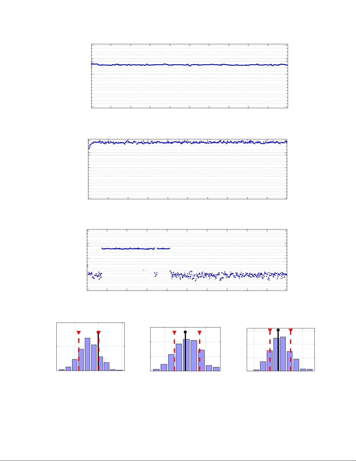
Be y ond T rans-dimensional RJMCMC: Application to Impulsive Data Modeling Oktay Karakus ¸ 1 , Ercan E. K uruo ˘ glu 2 , and Mustafa A. Altınkay a 1 1 ˙ Izmir Institute of T echnology (IZTECH), Electrical-Electronics Engineer ing, ˙ Izmir , T urkey 2 ISTI-CNR, via G. Moruzzi 1, 56124, Pisa, Italy ABSTRA CT Re versib le jump Mark ov chain Monte Car lo (RJMCMC) is a Bay esian model estimation method which has been used for trans-dimensional sampling. In this study , w e propose utilization of RJMCMC be yond trans-dimension al sampling. This ne w inter pretation, which we call trans-space RJMCMC , re veals the undisco v ered potential of RJMCMC by e xploiting the or iginal f or mulation to e xplore spaces of diff erent classes or structures. This provides fle xibility in using different types of candidate classes in the combined model space such as spaces of linear and nonlinear models or of various distribution families . As an application f or the proposed method, we ha ve perf or med a special case of trans-space sampling, namely trans-distrib utional RJMCMC in impulsive data modeling. In many areas such as seismology , radar , image, using Gaussian models is a common practice due to analytical ease. Howe ver , many noise processes do not f ollow a Gaussian character and generally exhibit e vents too impulsiv e to be successfully descr ibed by the Gaussian model. We test the proposed method to choose between various impulsiv e distribution f amilies to model both synthetically generated noise processes and real lif e measurements on power line communications (PLC) impulsive noises and 2-D discrete w avelet transf orm (2-D D WT) coefficients. 1 Introduction In v arious real-life modeling problems, we hav e limited prior information re garding which model f amily is more suitable for the problem. In such cases, a method that would allo w one to choose between different model families on the fly would be useful, eliminating the need for modeling with each candidate model class separately and comparing. This provides computational gains especially when the number of parameters and candidate model classes are high. An example is the choice between different pr obability density function (pdf) models for noise or signals. The pdf estimation problem is a frequently encountered problem in signal processing and statistics, and their application fields such as in image processing and telecommunications. In communication systems, channel modelling has been an important issue so as to characterize the whole system. Howe ver , for most of the cases, performing a deterministic channel modelling might be impossible and to represent real life systems, statistical channel models are very important. In addition, in applications of noise reduction operations in image processing, power -line communication systems, etc. dealing with a suitable statistical model beforehand is also important for the methods to be dev eloped. Despite this importance, estimating the correct (or suitable) probability distribution along with its parameters within a number of generic distrib ution models may necessitate testing each candidate in order to choose the best possible model for the observed data/noise. General tendency is to model noise/data with a Gaussian process especially in communications, network modeling, digital images, due to its analytical ease. In the case of non-Gaussian impulsive noise/data, v arious model families e xist, for example, Middleton Class A, Bernoulli-Gaussian, α -Stable, Generalized Gaussian (GG), Student’ s t, etc. It has been reported in the literature that noise exhibits non-Gaussian and impulsi ve characteristics in application areas such as wireless communications [ 1 , 2 ], power line communications (PLC) [ 3 , 4 ], digital subscriber lines (xDSL) [ 5 , 6 ], image processing [ 7 , 8 ] and seismology [9]. Reversible jump Markov chain Monte Carlo (RJMCMC) is a Bayesian model determination method which has had success in vast areas of applications since its introduction by Peter Green [ 10 ]. Unlike the widespread MCMC algorithm, Metr opolis-Hastings (MH), RJMCMC allows one to search in solution spaces of dif ferent dimensions which has been the main motiv ation for its use up to date. Classical applications of RJMCMC are model selection in regression and mixture processes [ 11 , 12 , 13 , 14 , 15 , 16 ]. Unlike the classical applications in the literature, the original formulation of RJMCMC in [ 10 ] permits a wider interpretation than just exploring the models with dif ferent dimensions. As an e xample of the applicability of RJMCMC beyond model dimension selection: it was utilized to learn polynomial autoregressi ve (P AR) [ 17 ], polynomial moving a verage (PMA) [ 18 ] and polynomial autoregressi ve moving av erage (P ARMA) [ 19 ] processes and identification of V olterra system models [20] by exploring linear and nonlinear model spaces in preliminary work by the authors. This paper contributes to the literature with a ne w interpretation on RJMCMC beyond trans-dimensional sampling, which we call trans-space RJMCMC . The proposed method uses RJMCMC in an unorthodox way and re veals its potential to be a general estimation method by performing the rev ersible jump mechanism between spaces of different model classes. T o demonstrate this potential, we focus our attention on a more special but generic problem of choosing between different probability distribution f amilies. The problem is a frequently encountered problem in signal processing and statistics, and their application fields such as in image processing and telecommunications. In this paper , we propose a Bayesian statistical modeling study of impulsi ve noise/data by estimating the probability distribution among three con ventional impulsi ve distributions families: symmetric α -Stable (S α S), GG and Student’ s t . Other than identifying the distribution family , the proposed method estimates shape and scale parameters of the distribution. These distributions are the most popular statistical models in applications cov ering diverse areas such as wireless channel modeling, financial time series analysis, seismology , radar imaging. W e study the algorithm extensi vely on synthetic data pro viding statistical significance tests. In addition, as case studies, we look into two statistical modeling problems of actual interest impulsi ve noise on PLC channels and 2-D discr ete wavelet transform (2-D DWT) coefficients. Particularly , PLC impulsi ve noise measurements in [ 21 , 22 ] have been utilized in the simulations. Apart from this, statistical modeling for 2-D DWT coef ficients ha ve been performed on dif ferent kinds of images such as Lena, synthetic apertur e radar (SAR) [23], magnetic r esonance imaging (MRI) [24] and mammogram [25]. Rest of the paper is organized as follows: general definitions for trans-dimensional RJMCMC and the proposed method are discussed in Section 2. Section 3 revie ws three distribution families and describes the impulsi ve data modeling scheme of the proposed method. Experimental studies for synthetically generated noise processes and for real applications are e xplained in Section 4. Section 5 draws conclusions on the results. 2 Rever sible jump MCMC RJMCMC has been first introduced by Peter Green in [ 10 ] as an extension of MCMC to a model selection method. Green, Green firstly deriv es the condition for the satisfaction of detailed balance requirements in terms of the Borel sets which the candidate models belong to. In the continuation of the deriv ation, he specializes his discussion to moves between spaces which differ only in dimensions and the general discussion is abandoned. In the follow up, to the best of our kno wledge almost all publications utilized RJMCMC for model dimension selection. Popular use of RJMCMC is in linear parametric models such as autor egr essive (AR) [ 11 ], autor egr essive inte grated moving aver age (ARIMA) [ 12 ] and fractional ARIMA (ARFIMA) [ 13 ] and mixture models such as Gaussian mixtures [14], Poisson mixtures [15] and α -stable mixtures [16]. Apart from the popular applications abov e, RJMCMC has been used in other various applications such as detection of clusters in disease maps [ 26 ], graphical models based variable selection and automatic curve fitting [ 27 ], log-linear model selection [ 28 ], non-parametric drift estimation [ 29 ], delimiting species using multilocus sequence data [ 30 ], random effect models [31], generation of lane-accurate road network maps from vehicle trajectory data [32]. In this study , our motiv ation is to propose a new interpretation on the classical RJMCMC beyond trans-dimensionality . The classical trans-dimensional RJMCMC of [10] and the proposed method, trans-space RJMCMC are discussed in the sequel. 2.1 T rans-dimensional RJMCMC The standard MH algorithm [33] accepts a transition from Markov chain state x ∈ X to y ∈ X with a probability of: A ( x → y ) = min  1 , π ( y ) q ( x , y ) π ( x ) q ( y , x )  (1) where π ( · ) represents the target distribution and q ( y , x ) refers to the proposal distrib ution from state x to y . RJMCMC, in the sense of trans-dimensional MCMC, generalizes MH algorithm by defining multiple parameter subspaces ζ k of dif ferent dimensionality [ 10 ]. This is only achie ved by defining dif ferent types of mo ves between subspaces pro viding that the detailed balance is attained. For this condition to hold, a re verse mov e from state y to x should be defined and dimension matching should be satisfied between parameter subspaces. Assume that we propose a move m with probability p m from a Markov chain state κ to κ 0 each of which has parameter vectors θ ∈ ζ 1 and θ 0 ∈ ζ 2 , respectiv ely with different dimensions. The mov e m is re versible and its reverse move m R is proposed with a probability p m R . The general detailed balance condition can be stated as: π ( κ ) q ( κ 0 , κ ) A ( κ → κ 0 ) = π ( κ 0 ) q ( κ , κ 0 ) A ( κ 0 → κ ) , (2) where proposal distrib ution q ( · ) is directional and includes the probabilities of both the mo ve itself and the proposed parameters. Then, the general expression for the acceptance ratio in (1) turns into [10]: 2/22 (3) A ( κ → κ 0 ) = min  1 , π ( κ 0 ) p m R χ 2 ( u 0 ) π ( κ ) p m χ 1 ( u )     ∂ ( θ 0 , u 0 ) ∂ ( θ , u )      , where χ 1 ( · ) and χ 2 ( · ) are the distrib utions for the auxiliary v ariable vectors u and u 0 , respecti vely which are required to pro vide dimension matching for the mov es m and m R . The term    ∂ ( θ 0 u 0 ) ∂ ( θ , u )    is the magnitude of the Jacobian. In each RJMCMC run, the standard Metropolis-Hastings algorithm is applied in mo ves within the same dimensional models, which is called as life move. Sampling is performed in a single parameter space and there is no dimension change in life mov e. For trans-dimensional transitions between models, mo ves such as birth , death , split and mer ge are performed which require the creation or the deletion of new v ariables corresponding to the increased or decreased dimension. Green handles the dimension changing mov es as variable transformations and defines a dummy v ariable to match dimensions which provides a square Jacobian matrix that can be used to update the acceptance ratio easily . 2.2 T rans-space RJMCMC In spite of RJMCMC’ s use in trans-dimensional cases, the original formulation in [ 10 ] holds a wider interpretation than just sampling between spaces of different dimensions. In the beyond trans-dimensional RJMCMC point of view , the main requirements of RJMCMC stated by Green are still valid with one e xception, that is, a change in parameter space definition. In the original formulation, Green firstly derives the condition for the satisfaction of detailed balance requirements in terms of the Borel sets which the candidate models belong to. In the continuation of the deriv ation, he specializes his discussion to mov es between spaces which dif fer only in dimensions and the general discussion is abandoned. Howe ver , the parameter vectors in (2) may belong to Borel sets which dif fer not only in their dimensions but also in the generic models the y belong to. Thus, the algorithm can be used for much more generic implementations. Notwithstanding, this general interpretation should be taken with caution to ha ve a useful method. Particularly , the Borel sets should be r elated somehow , which can be con veniently set by matching a common pr operty (e.g . norm) in defining the spaces. Defining proposals in this w ay will provide sampling more ef ficient candidates and help algorithm to con verge faster . As an example, model transitions can be designed to pro vide fixed first ordered moments between spaces. Thus, this moment based approach provides a more ef ficient way to explore all the candidate models within the combined space. Carrying the trained information to a ne w generic model space is very crucial in this frame work. Otherwise, the algorithm would start to train from scratch repeatedly each time it changes states and sampling across unrelated spaces would not gi ve us a computational advantage. In that case, one could solve for dif ferent spaces separately and compare the final results to choose the best model. T wo examples one can think of firstly , are: 1. κ might correspond to a linear parametric model such as AR while κ 0 might correspond to a nonlinear model such as V olterra AR. 2. κ might correspond to a pdf p A with certain distribution parameters while κ 0 might correspond to another pdf p B with some other distribution parameters. T o this end, we define a combined parameter space ϕ = S k ϕ k for k > 1 . Assume that a mov e M from Markov chain state x ∈ ϕ 1 to x 0 ∈ ϕ 2 is defined and Borel sets A ⊂ ϕ 1 and B ⊂ ϕ 2 are related with a set of functions each of which are inv ertible. Particularly , for any Borel sets in both of the spaces, ϕ 1 and ϕ 2 , functions h 12 : A 7→ B and h 21 : B 7→ A can be defined by matching a common property of the spaces. For generality , if the proposed mov e requires matching the dimensions, auxiliary variables u 1 and/or u 2 can be drawn from proper densities Q 1 ( · ) and Q 2 ( · ) , respecti vely . Otherwise, one can set u 1 and u 2 to / 0 . Please note that the dimensions of the parameter spaces at both sides of the transitions can be different or the same and rev ersible jump mechanism is still applicable. Consequently , although the candidate spaces are of dif ferent classes, since the Borel sets are defined as to be related, the assumption of Green still holds for a symmetric measure ξ m and densities for joint proposal distributions, π ( · ) q ( · , · ) , can be defined with respect to this symmetric measure by satisfying the equilibrium in (2). Thus, the acceptance ratio can be written as: (4) A ( x → x 0 ) = min  1 , π ( x 0 ) p M R Q 2 ( u 2 ) π ( x ) p M Q 1 ( u 1 )     ∂ h 12 ( θ 1 , u 1 ) ∂ ( θ 1 , u 1 )      . where M R is the rev erse move of M and p M and p M R represent the probabilities of the moves. The Jacobian term appears in the equation as a result of the change of variables operation between spaces. Here we recall that in our previous works [ 17 , 18 , 19 , 20 ], we hav e performed model estimation studies with RJMCMC for V olterra based nonlinear models P AR, PMA and P ARMA as well as an identification study of V olterra system models. In these studies, RJMCMC has been utilized to explore the model spaces of linear and nonlinear models in polynomial sense instead of performing a model order selection study in a single linear model space. Hence, we add a fe w concluding remarks. 3/22 Remark1. W e are going to name this new utilization on RJMCMC as trans-space rather than trans-dimensional . Trans-space RJMCMC rev eals a general framework for exploring the spaces of dif ferent generic models whether or not their parameter spaces are of different dimensionality . Consequently , trans-dimensional case is a subset of trans-space transitions. Remark2. T rans-space RJMCMC requires to define new types of mov es due to the need for more detailed operations than, e.g. just being birth, death, split and merge of the parameters. These moves will be named as between-space moves and may include both birth and death of the parameters at the same time or a norm based mapping between the parameter spaces. Switch mo ve (firstly proposed for V olterra system identification study [ 20 ]) will be proposed as a between-space mo ve, which performs a switching between the candidate spaces of the generic model classes. Remark3. As a special case of trans-space sampling, the proposed method can be used to explore the spaces of different distribution f amilies. Therefore, this special case will be named as trans-distrib utional . 3 T rans-distributional RJMCMC for Impulsive Distrib utions In this study , we hav e applied RJMCMC to problems in which a stochastic process, x , is giv en whose impulsiv e distribution is to be found. For this purpose, we define a reversible jump mechanism which estimates the distribution family among three impulsiv e distribution families, namely , S α S, GG and Student’ s t . These three families cov er many different noise modeling studies as stated in the above sections. All of them include Gaussian distribution as a special member , and many real life noise measurements can be modelled with these distribution families. For example, S α S family has various demonstrated application areas such as PLC [ 34 ], SAR imaging [ 8 ], near optimal receiv er design [ 35 ], modelling of counterlet transform subbands [ 36 ], seismic amplitude data modelling [ 9 ], as noise model for molecular communication [ 37 ], reconstruction of non-negati ve signals [ 38 ] (Please see [ 39 ] and references therein for detailed applications). GG distributions have found applications in wav elet based texture retriev al [ 40 ], image modelling in terms of Markov random fields [ 41 ], multicomponent texture discrimination in color images [ 42 ], wheezing sound detection [ 43 ], modelling sea-clutter data [44]. Student’ s t distribution is an alternati ve to Gaussian distribution especially for small populations where the v alidity of central limit theorem is questionable. Student’ s t distribution has been used in applications of finance [ 45 , 46 ], full-wa veform in version of seismic data [ 47 ], independent vector analysis for speech separation [ 48 ], medical image se gmentation [ 49 ], gro wth curve modelling [50]. One might argue that training separate MCMC samplers for each of the seemingly irrelev ant distribution families and comparing their modelling performances afterw ards would be computationally more adv antageous. Ho wev er, in cases when the number of candidate models is not kno wn or dramatically large, implementing a single Marko v chain via RJMCMC could be simpler . In addition, when the number of models are small, one can not conclude that parallel MCMC approach would be a better choice than RJMCMC and this requires an analysis. By efficiently choosing the proposal distributions, the adv antage of incorporating rev ersible jump mechanism can be extended to searching several distrib ution families which will be described in the sequel. In the literature, RJMCMC usage in this problem has been limited and it has been used to be examples of trans-dimensional approach deciding between two specific distributions [ 51 , 52 ]. P articularly , when modelling count data, re versible jump mechanism has been applied to choose between Poisson and negati ve binomial distributions in [ 51 ]. This study deals with the question whether the count data is ov er-dispersed relati ve to Poisson distribution. In [ 52 ] an approach which is a combination of Gibbs sampler and RJMCMC has been used to decide between Poisson and geometric distributions by using a univ ersal parameter space called “palette”. Both of the studies have utilized RJMCMC in distrib ution estimation; howe ver , the number of candidate distributions was limited to two. Moreover , in both of the studies, Poisson distrib ution is a special member of the distribution f amilies in question (or , there is a direct relation between Poisson and negati ve binomial or geometric distrib utions), hence, the methods in these studies can be handled with a single family search. The proposed method, trans-distributional RJMCMC, is much more general than the examples above and aims to fit a distribution to a gi ven process x among v arious distributions by identifying the distrib ution’ s family and estimating its shape and scale parameters. T wo types of between-class mov es hav e been defined, namely intra-class-switch and inter -class-switch . These mov es propose model class changes within and between probability distribution f amilies, respectiv ely . 3.1 Impulsive Distribution F amilies 3.1.1 Symmetric α -Stable Distribution Family There is no closed form expression for probability density function (pdf) of S α S distributions e xcept for the special cases of Cauchy and Gaussian. Howe ver , its characteristic function, ϕ ( x ) , can be expressed explicitly as: 4/22 ϕ ( x ) = exp ( j δ x − γ | x | α ) (5) where 0 < α ≤ 2 is the characteristic exponent, a.k.a. shape parameter , which controls the impulsi veness of the distribution. Special cases Cauchy and Gaussian distributions occur when α = 1 and α = 2 , respecti vely . − ∞ < δ < ∞ represents the location parameter . The γ > 0 provides a measure of the dispersion which is the scale parameter expressing the spread of the distribution around δ . 3.1.2 Generalized Gaussian Distribution Family The univ ariate GG pdf can be defined as: f ( x ) = α 2 γ Γ ( 1 / α ) exp  −  | x − δ | γ  α  (6) where Γ ( · ) refers to the gamma function, α > 0 is the shape parameter , − ∞ < δ < ∞ represents the location parameter and the γ > 0 is the scale parameter . GG family has well-known members such as Laplace, Gauss and uniform distributions for α values of 1, 2 and ∞ , respecti vely . 3.1.3 Student’ s t Distribution Family The uni variate symmetric Student’ s t distribution f amily is an impulsi ve distribution f amily with parameters, α > 0 which is the number of degrees of freedom, a.k.a shape parameter , the location parameter − ∞ < δ < ∞ and the scale parameter γ > 0 . Its pdf can be defined as: f ( x ) = Γ  α + 1 2  Γ ( α / 2 ) γ √ π α 1 + 1 α  x − δ γ  2 ! − (( α + 1 ) / 2 ) . (7) Special members of the symmetric Student’ s t distribution family are Cauchy and Gauss which are obtained for shape parameter values of α = 1 and α = ∞ , respectiv ely . 3.2 P arameter Space RJMCMC construction for impulsi ve data modeling be gins by firstly defining the parameter space. Parameter space has been defined on the common parameters for all three distribution families. These are: shape, scale and location parameters ( α , γ and δ , respectiv ely). In addition to them, the family identifier , k , which defines the estimated distribution family has been added to the parameter space. The k values of the distributions S α S, GG and Student’ s t are 1, 2 and 3, respectively . Therefore, the parameter vector θ can be formed as: θ = { k , α , δ , γ } . In this study , the observed data from all three families are assumed to be symmetric around the origin for simplicity . Therefore, δ , is set to 0 and its effect will be invisible in the simulations. Consequently , parameter vector θ is reduced to: θ = { k , α , γ } . 3.3 Hierarc hical Bay esian Model The target distrib ution, f ( θ | x ) , can be decomposed to likelihood times priors due to Bayes Theorem as: f ( θ | x ) ∝ f ( x | k , α , γ ) f ( α | k ) f ( k ) f ( γ ) . (8) where f ( x | k , α , γ ) represents the likelihood and f ( α | k ) , f ( k ) , and f ( γ ) are the priors. 3.4 Likelihood W e assume that the stochastic process x with a length of n comes from one of the distributions in candidate families (S α S, GG and Student’ s t ). Then, the likelihood corresponds to a pdf from one of these distributions: f ( x | k , α , γ ) =    ∏ n i = 1 S α S ( γ ) , k = 1 ∏ n i = 1 GG α ( γ ) , k = 2 ∏ n i = 1 t α ( γ ) , k = 3 (9) 5/22 3.5 Priors Priors hav e been selected as the following: f ( γ ) = I G ( a , b ) , (10) f ( k ) = I { 1 / 3 , 1 / 3 , 1 / 3 } for k = 1 , 2 , 3 , (11) f ( α | k ) =    U ( 0 , 2 ) k = 1 , U ( 0 , α max,GG ) k = 2 , U ( 0 , α max , t ) k = 3 , (12) where a and b represent the hyperparameters for scale parameter and they are generally selected as to take small values such as 1 , 0 . 1 in the literature. The upper bounds for the shape parameters of GG and Student’ s t distributions ha ve been defined as α max,GG and α max , t , respectiv ely . Choosing an inv erse gamma prior for scale parameter is a general practice especially for Gaussian problems. Due to the lack of information about conjugate priors for distributions other than the Gaussian case and since Gaussian distribution is common for all three families, an in verse gamma conjug ate prior for scale parameters has been chosen for simplicity . Furthermore, all families are equiprobable a priori and shape parameter is uniformly distrib uted between lo wer and upper bounds. 3.6 Model Moves T wo RJMCMC model mov es ha ve been defined in order to perform trans-distrib utional transitions discussed in the pre vious sections. These are: life and switch moves. Life move performs classical MH algorithm to update γ . Switch move performs exploring the other distrib ution spaces. For this purpose, two types of switch mo ves ha ve been defined: intra-class-switch and inter-class-switc h . Intra-class-switch performs exploring the distributions in the same family , while inter-class-switch explores spaces of different families. At each RJMCMC iteration, one of the moves is chosen with probabilities P life , P intra-cl-sw and P inter-cl-sw , respectiv ely . In Figure 1 the flow diagram of the proposed method is depicted where the parameter N refers to the maximum number of iterations. The details about the steps of the selected mov es are discussed in the sequel. 3.6.1 Life Move Life mo ve defines a transition from parameter space ( k , α , γ ) to ( k 0 , α 0 , γ 0 ) and only proposes a candidate for the scale parameter , γ ( α 0 = α and k 0 = k ). The proposal distribution for scale parameter γ 0 has been chosen as: q ( γ 0 | γ ) = T N ( γ , ξ scal e ) for interval ( 0 , γ + 1 ] (13) where T N ( γ , ξ scal e ) refers to a Gaussian distribution where its mean γ is the last v alue of the scale parameter , and its variance is ξ scal e and is truncated to lie within the interval of ( 0 , γ + 1 ] afterwards by rejecting samples outside this interval. This truncation procedure aims to satisfy the condition γ > 0 and forces candidate proposals not to lie f ar from the last v alue of γ . Hence, the resulting acceptance ratio for life mov e is: A life = min  1 , f ( x | k 0 , α 0 , γ 0 ) f ( x | k , α , γ ) f ( γ 0 ) f ( γ ) q ( γ | γ 0 ) q ( γ 0 | γ )  (14) 3.6.2 FLOM Based Proposals for γ T ransitions As mentioned earlier in this paper , using a common feature among the candidate model spaces for the transition to be made will provide ef ficient proposals and is important in order to link the subspaces of different classes. Assume we hav e two candidate families parameter v ectors of which belong to Borel sets, A and B , respecti vely . Providing fix ed order norm for both of the Borel sets, the transition (e.g. h : A 7→ B ) from one set to another carries the information in the same direction which h as been already learned at the most recent Borel set. Considering the con ver gence and mixing of the algorithm, such an approach is very important to determine the transition process between generic distribution models, whether within the family or between families. When dealing with distribution estimation problems, moments with various orders, p hav e been defined for all distribution families. Moments of t and GG families ha ve been defined at an y orders for p > 0 and there are no restrictions on values of p . Ho wev er, moments of the S α S family hav e been defined subject to the constraint of p < α . This constraint makes it possible to use the absolute fractional lower or der moments (FLOMs) which has been also used in the parameter estimation methods of the S α S family . By taking into consideration of the facts that absolute FLOM expressions are defined for all impulsi ve f amilies, 6/22 Figure 1. Flo w Diagram for the Proposed method. and their success in parameters estimation studies of the S α S distributions, using an absolute FLOM based approach helps to construct a reversible jump sampler between different impulsiv e families, by linking the candidate distributions through absolute FLOM. In impulsiv e data modelling study in this study , absolute FLOM-based approach will be used for the proposals of the γ parameter . In particular , to perform sampling between related subspaces and generate efficient proposals on scale parameter γ , an absolute FLOM-based method has been used. The newly proposed scale parameter, γ 0 , is calculated via a re versible function, g ( · ) (or w ( · ) ), which provides equal absolute FLOMs with order p for both the most recent and candidate distrib ution spaces. Thus, proposals on γ carry the learned information to the candidate space via absolute FLOMs. Absolute FLOMs are defined only for p values lo wer than alpha for the case of S α S distributions. Moreover , there are several studies which suggest near-optimum values for FLOM order p in order to estimate the scale parameter of S α S distributions. [ 53 ] suggests p = α / 4 and [ 54 ] suggests p = 0 . 2 . Howe ver , in [ 55 ] it has been stated that decreasing p for a fixed v alue of α (i.e. increasing α / p ), increases the estimation performance of γ and [ 55 ] suggests the choice p = α / 10 . W e use the value p = α / 10 in our simulations for all the distribution families. For a gi ven data, x , in order to perform a transition from parameter space { k , α , γ } to { k 0 , α 0 , γ 0 } we assume that the absolute FLOM will be the same for both the most recent and candidate distribution spaces. In particular , E k ( | x | p ) = E k 0 ( | x | p ) (15) where absolute FLOMs for all three candidate families can be defined as: 7/22 E k ( | x | p ) =    C α ( p , α ) γ p / α k = 1 , C GG ( p , α ) γ p k = 2 , C t ( p , α ) γ p k = 3 , (16) where C α ( p , α ) = Γ  p + 1 2  Γ  − p α  α √ π Γ  − p 2  2 p + 1 , (17) C GG ( p , α ) = Γ  p + 1 α  Γ ( 1 / α ) , (18) C t ( p , α ) = Γ  p + 1 2  Γ  α − p 2  √ π Γ  α 2  α p / 2 . (19) The candidate proposal, γ 0 , has been calculated via re versible functions which are deri ved by using the relations in (15)-(19) for each transition. These functions ha ve been deri ved for both of the switch moves and are sho wn in T ables 1 and 2. 3.6.3 Intra-Class-Switch Move RJMCMC performs a transition on shape and scale parameters in the same distribution family ( k 0 = k ) when an intra-class- switch mov e is proposed. The proposed shape parameter α 0 is sampled from a proposal distribution q ( α 0 | α ) . In addition, the candidate scale parameter γ 0 is defined as a function g ( α , α 0 , p , γ ) . The γ transition in this move has been defined as dependent on the ne wly proposed α 0 parameter . For this reason, a step is first performed on shape parameter α to propose α 0 , and this is used to calculate the candidate scale parameter γ 0 . For the shape parameter α transition, a proposal distrib ution such as q ( α 0 | α ) has been used. For this distrib ution, we first ha ve assumed a symmetric distribution around the most recent α value. In addition, it has been preferred that the proposal distribution has heavier tails than Gaussian in order to make it possible to sample candidates much farther than the most recent α relati ve to the samples from the Gaussian distrib ution. Since the Laplace distribution is a distrib ution that satisfies all these conditions, the proposal distribution is chosen as a Laplace distribution. Due to the numerical calculation problems caused when α and α 0 are close to each other (i.e. | α − α 0 |≤ 0 . 03 ), we hav e decided to utilize a finite number of candidate distributions (i.e. a finite number of α values) and the space on α is discretized with increments of 0.05. That’ s why a discretized Laplace ( D L ( α , Γ ) ) distribution where the location parameter of which is equal to the most recent shape parameter α and scale parameter is Γ , has been utilized. An example figure of the proposal distrib ution q ( α 0 | α ) is shown in Figure 2(a). Importantly , our choice on the proposal distrib ution q ( α 0 | α ) is not restricti ve; an y distribution other than Laplace can be selected as the proposal distrib ution (e.g. Gaussian like). Howe ver , different selections will cause the algorithms to perform differently . Candidate scale parameter γ 0 has been calculated via reversible functions, g ( · ) , which are derived for intra-class-switch mov e by using the method in Section 3.6.2. Functions for each family are sho wn in T able 1. Consequently , proposals for intra-class-switch mov e are; q ( α 0 | α ) = D L ( α , Γ ) , (20) γ 0 = g ( α , α 0 , p , γ ) . (21) As a result of the details explained abo ve, acceptance ratio for RJMCMC intra-class-switch mo ve can be e xpressed as; A intra-cl-sw = min  1 , f ( x | k 0 , α 0 , γ 0 ) f ( x | k , α , γ ) f ( γ 0 ) f ( γ ) | J |  , (22) where | J | is the magnitude of the Jacobian (See T able 1). 8/22 0 0.5 1 1.5 2 Candidate Shape parameter 0 0.02 0.04 0.06 0.08 Probability (a) 0 0.5 1 1. 5 2 Shape parameter for Stable Dist. 0 2 4 6 Candidate Shape parameter f 1 (alpha) f 2 (alpha) (b) Figure 2. (a) - Proposal distribution, q ( α 0 | α ) for intra-class-switch mov e ( γ = 1 , Γ = 0 . 4 ) . (b) - Mapping functions on shape parameter for inter-class-switch mo ve T able 1. Intra-Class-Switch Details [ ( k , α , γ ) → ( k 0 , α 0 , γ 0 ) ] Family Degree, p γ 0 = g ( α , α 0 , p , γ ) Jacobian, | J | S α S α 0 / 10  C α ( p , α ) C α ( p , α 0 )  α 0 / p γ α 0 / α  C α ( p , α ) C α ( p , α 0 )  α 0 / p α 0 α γ ( α 0 − α ) / α GG α 0 / 10  C GG ( p , α ) C GG ( p , α 0 )  1 / p γ  C GG ( p , α ) C GG ( p , α 0 )  1 / p t α 0 / 10  C t ( p , α ) C t ( p , α 0 )  1 / p γ  C t ( p , α ) C t ( p , α 0 )  1 / p T able 2. Inter -Class-Switch Details [ ( k , α , γ ) → ( k 0 , α 0 , γ 0 ) ] ( k → k 0 ) Degree, p α 0 = ψ ( α , k , k 0 ) γ 0 = w ( α , α 0 , p , γ ) 1 → 2 α 0 / 10 f 1 ( α ) = α 2 2  C α ( p , α ) C GG ( p , α 0 )  1 / p γ 1 / α 1 → 3 α 0 / 10 f 2 ( α ) = l ogit  α + 2 4   C α ( p , α ) C t ( p , α 0 )  1 / p γ 1 / α 2 → 1 α 0 / 10 f − 1 1 ( α )  C GG ( p , α ) C α ( p , α 0 )  α 0 / p γ α 0 2 → 3 α 0 / 10 f 2 ( f − 1 1 ( α ))  C GG ( p , α ) C t ( p , α 0 )  1 / p γ 3 → 1 α 0 / 10 f − 1 2 ( α )  C t ( p , α ) C α ( p , α 0 )  α 0 / p γ α 0 3 → 2 α 0 / 10 f 1 ( f − 1 2 ( α ))  C t ( p , α ) C GG ( p , α 0 )  1 / p γ 3.6.4 Inter-Class-Switch Move Dif ferent from intra-class-switch move, distrib ution family has also been changed in inter-class-switch move ( k 0 6 = k ) as well as scale and shape parameters. Candidate distribution families are equiprobable for the candidate set { 1 , 2 , 3 }\{ k } , and we use functions below to propose candidate parameters of α 0 and γ 0 . α 0 = ψ ( α , k , k 0 ) (23) γ 0 = w ( α , α 0 , p , γ ) (24) 9/22 For intra-class transitions mentioned in the section abo ve, the kno wledge (about scale γ ) learned in the previous algorithm steps was carried to the ne xt step by the proposed method via FLOM based functions. The same approach is also utilized for γ transitions in inter-class-switch move and functions w ( · ) are deriv ed, howe ver , this time, the sides of the transition are in different f amilies. Details are shown in T able 2. In order to perform efficient proposals for α in inter-class-switch mov e, instead of using a random move, we perform a mapping, ψ ( · ) from one family to another by taking into consideration the special members which are common for both of the families. For e xample, to deri ve an inv ertible mapping function on α for a transition from S α S to Student’ s t , we utilize the information that Cauchy and Gauss distrib utions are common for both of the families. Cauchy refers to α = 1 for both of the families and Gauss refers to α = 2 for S α S and α = ∞ for Student’ s t . Hence, the in vertible function f 2 ( α ) performs the mapping for a transition from S α S to Student’ s t . Similarly , Gauss distribution is common for both S α S and GG for α v alue of 2. Thus, we deriv e another in vertible function f 1 ( α ) to move from S α S to GG. Both of these mapping functions hav e been depicted in Figure 2(b). GG and Student’ s t distributions ha ve only Gauss distribution in common for α values of 2 and ∞ , respectiv ely . Due to having only one common distribution and infinite range of α , instead of deriving an in vertible mapping for transitions between these distributions, we perform a 2-stage mapping mechanism by firstly mapping α to S α S from the most recent family , then mapping this value to the candidate family by using functions f 1 ( · ) or f 2 ( · ) . Then the mapping from GG to Student’ s t is deriv ed as: α 0 = f 2 ( f − 1 1 ( α )) . It is straightforward to show that the re verse transition between shape parameters from Student’ s t to GG results as α 0 = f 1 ( f − 1 2 ( α )) . For all the transitions, mapping functions hav e been sho wn in T able 2. So, the acceptance ratio for inter-class-switch mo ve can be expressed as: A inter-cl-sw = min  1 , f ( x | k 0 , α 0 , γ 0 ) f ( x | k , α , γ ) f ( γ 0 ) f ( γ ) f ( α | k ) f ( α 0 | k 0 ) | J |  (25) where | J | = ∂ γ 0 ∂ γ ∂ α 0 ∂ α . 4 Experimental Study W e study experimentally three cases: synthetically generated noise, impulsi ve noise on PLC channels and 2-D DWT coefficients. W ithout loss of generality , distribution of data x is assumed to be symmetric around zero ( δ = 0 ). The algorithm starts with a Gaussian distribution model with initial v alues k ( 0 ) = 2 and α ( 0 ) = 2 . Initial v alue for scale parameter γ is selected as half of the interquartile range of the giv en data x and upper bounds α max,S α S , α max,GG and α max , t are selected as 2, 2 and 5, respecti vely . Some intuitiv e selections have been performed for the rest of the parameters. Mov e probabilities for intra-class-switch and inter-class-switch moves are assumed to be equally likely during the simulations. Additionally , in order to speed up the con vergence of the distrib ution parameter estimations during the life move, which is the coef ficient update move, it is chosen a bit more likely than intra-class-switch and inter-class-switch moves. Thus, the model mov e probabilities are selected as P life = 0 . 4 , P intra-cl-sw = 0 . 3 and P inter-cl-sw = 0 . 3 . Hyperparameters for prior distrib ution of γ are set to a = b = 1 and v ariance of proposal distribution for γ in life mov e is set to ξ scal e = 0 . 01 . Scale parameter Γ of the discretized Laplace distribution for intra-class-switch mov e is selected as 0.4. RJMCMC performs 5000 iterations in a single RJMCMC run and half of the iterations are discarded as burn-in period when estimating the distrib ution parameters. Random numbers from all the families ha ve been generated by using Matlab’ s Statistics and Machine Learning T oolbox (for details please see 1 ). Performance comparison has been performed under two statistical significance tests, namely K ullback-Leibler (KL) div ergence and K olmogor ov-Smirnov (KS) statistics. KL div ergence has been utilized to measure fitting performance of the proposed method between estimated pdf and data histogram. T wo-sample KS test compares empirical CDF of the data and the estimated CDF . It quantifies the distance between CDFs and performs an hypothesis test under a null h ypothesis that two samples are drawn from the same distrib ution. Details about KL diver gence and KS test have been discussed in Appendix A. 4.1 Case Study 1: Synthetically Generated Noise Modeling In order to test the proposed method on modeling synthetically generated impulsiv e noise processes, six different distrib utions are chosen (2 distrib utions from each family). In a single RJMCMC run, data with a length of 1000 samples have been generated from one of the example distrib utions. The example distributions are S 1 S ( 0 . 75 ) , S 1 . 5 S ( 2 ) , GG 0 . 5 ( 0 . 5 ) , GG 1 . 7 ( 1 . 4 ) , t 3 ( 1 ) and t 0 . 6 ( 3 ) . 1 https://www.mathworks.com/help/stats/continuous- distributions.html 10/22 0 500 1000 1500 2000 2500 3000 3500 4000 4500 5000 Iteration 5 0 2 0 2 ---------- GenGauss ---------- ---------- Stable ---------- Student ----------- (a) S1 . 5S ( 2 ) 0 500 1000 1500 2000 2500 3000 3500 4000 4500 5000 Iteration 5 0 2 0 2 ------------ GenGauss ------------ Stable ------------ Student ------------ (b) GG 1 . 7 ( 1 . 4 ) 0 500 1000 1500 2000 2500 3000 3500 4000 4500 5000 Iteration 5 0 2 0 2 ------------ GenGauss ------------ Stable ------------ Student ------------ (c) t 3 ( 1 ) 1.8 2 2.2 Estimated Scale 0 0.2 0.4 Probability (d) S1 . 5S ( 2 ) 1.3 1.4 1.5 Estimated Scale 0 0.1 0.2 0.3 Probability (e) GG 1 . 7 ( 1 . 4 ) 0.9 1 1.1 Estimated Scale 0 0.1 0.2 0.3 Probability (f) t 3 ( 1 ) Figure 3. Synthetically generated noise modeling - parameter estimation results in a single RJMCMC run. (a),(b),(c): Instantaneous α estimates. (d),(e),(f): Estimated posterior distributions for γ after b urn-in period. 11/22 T able 3. Modeling results for synthetically generated processes. Distribution Est. Est. Est. KL Div . KS KS Distribution Family Shape ( ˆ α ) Scale ( ˆ γ ) Score p -value S1 . 5S ( 2 ) S α S 1.4769 1.9162 0.0169 0.0125 1.0000 S1S ( 0 . 75 ) t 0.9970 0.7300 0.0454 0.0489 > 0 . 9999 GG 0 . 5 ( 0 . 5 ) GG 0.4990 0.5199 0.0229 0.0152 1.0000 GG 1 . 7 ( 1 . 4 ) GG 1.6456 1.3374 0.0221 0.0202 1.0000 t 3 ( 1 ) t 2.9303 1.0039 0.0251 0.0203 1.0000 t 0 . 6 ( 3 ) t 0.6197 2.9869 0.0465 0.0452 > 0 . 9999 T able 4. Modeling results for PLC impulsi ve noise. Data Est. Est. Est. KL Div . KS KS F amily Shape ( ˆ α ) Scale ( ˆ γ ) Score p -value PLC-1 S α S 1.2948 5.6969 0.0086 0.0112 1.0000 PLC-2 S α S 0.7042 0.1799 0.0441 0.0486 > 0 . 9999 PLC-3 S α S 1.3140 1.3488 0.0046 0.0132 1.0000 T able 5. Modeling results for 2D-D WT coefficients. Image Est. Est. Est. KL Div . KS KS Family Shape ( ˆ α ) Scale ( ˆ γ ) Score p -v alue Lena (V) GG 0.5002 1.7415 0.0271 0.0465 > 0 . 9999 Lena (H) t 1.0958 2.2422 0.0094 0.0349 > 0 . 9999 Lena (D) t 1.1628 1.7735 0.0145 0.0271 1.0000 SAR(V) S α S 1.5381 7.7395 0.0025 0.0123 1.0000 SAR(H) S α S 1.4500 8.6249 0.0043 0.0221 1.0000 SAR(D) S α S 1.7500 6.3710 0.0062 0.0125 1.0000 MRI(V) GG 0.3913 0.2693 0.0365 0.1152 0.8744 MRI(H) GG 0.3527 0.1039 0.0305 0.0548 > 0 . 9999 MRI(D) S α S 0.8504 0.5184 0.0245 0.0659 0 . 9998 Mammog.(V) t 1.6325 1.6411 0.0363 0.0907 0.9816 Mammog.(H) GG 0.7501 1.5154 0.0121 0.0555 > 0 . 9999 Mammog.(D) t 1.6430 0.4851 0.0073 0.0117 1.0000 40 RJMCMC runs have been performed for each distribution and estimated families with shape and scale parameters for each example distrib ution are shown in T able 3. In Figure 3, instantaneous estimate of shape parameter α and estimated posterior distrib ution of scale parameter γ are sho wn for three example distrib utions. Results represent the estimates obtained by a randomly selected RJMCMC run out of 40 runs. Burn-in period is not removed in the subfigures (a)-(c) in order to show the transient characteristics of the algorithm. These plots show that the proposed method con ver ges to the correct shape parameters. In subfigures (d)-(f), vertical dashed-lines with ∇ markers refer to ± σ confidence interval (CI). Examining these subfigures shows that correct scale parameters lie within the ± σ CI of the posteriors. Estimated pdfs and CDFs for three example distributions are depicted in Figure 4. In addition to the statistical significance values in T able 3, fitting performance of the algorithm has been presented visually . As can be seen in Figure 4, estimated pdfs are very similar to the data histogram and fitting performances for all e xample distributions lie within KL distance of at most 0.0465. Moreover , estimated CDFs under KS statistic score are also very low and p -values are close to 1,0000. Please note that the estimation result in the second line of T able 3 is meaningful for an example Cauchy distribution, since the Cauchy distribution is a special member in both S α S and Student’ s t families. 4.2 Case Study 2: Modelling Impulsive Noise on PLC Systems PLC is an emerging technology which utilizes po wer-lines to carry telecommunication data. T elecommunication speeds up to 200 Mb/s with a good quality of service can be achiev ed on PLC systems. Apart from this, PLC of fers a physical medium for indoor multimedia data traffic without additional cables [34]. A PLC system has v arious types of noise arising from electrical de vices connected to power line and e xternal effects via 12/22 -60 -40 -20 0 20 40 60 Samples 0 0.05 0.1 0.15 0.2 0.25 0.3 0.35 Probability Data Histogram Estimated pdf (a) S1 . 5S ( 2 ) -60 -40 -20 0 20 40 60 Samples 0 0.2 0.4 0.6 0.8 1 Probability Emprical CDF Estimated CDF (b) S1 . 5S ( 2 ) -4 -2 0 2 4 Samples 0 0.02 0.04 0.06 0.08 Probability Data Histogram Estimated pdf (c) GG 1 . 7 ( 1 . 4 ) -4 -2 0 2 4 Samples 0 0.2 0.4 0.6 0.8 1 Probability Estimated CDF Emprical CDF (d) GG 1 . 7 ( 1 . 4 ) -15 -10 -5 0 5 10 15 Samples 0 0.05 0.1 0.15 0.2 Probability Data Histogram Estimated pdf (e) t 3 ( 1 ) -15 -10 -5 0 5 10 15 Samples 0 0.2 0.4 0.6 0.8 1 Probability Estimated CDF Emprical CDF (f) t 3 ( 1 ) Figure 4. Synthetically generated noise modeling results. (a)-(c): Estimated pdfs, (d)-(f): Estimated CDFs. 13/22 0 1 2 3 4 5 Time in ms -200 -100 0 100 200 Noise Amplitude in mV (a) PLC-1 0 1 2 3 4 Time in us -5 0 5 Noise Amplitude in mV (b) PLC-2 0 5 10 15 20 25 30 35 Time in us -40 -20 0 20 40 Noise Amplitude in mV (c) PLC-3 -200 -100 0 100 200 Samples 0 0.05 0.1 0.15 0.2 Probability Data Histogram Estimated pdf (d) PLC-1 -5 0 5 Samples 0 0.1 0.2 0.3 0.4 0.5 Probability Data Histogram Estimated pdf (e) PLC-2 -40 -20 0 20 40 Samples 0 0.05 0.1 0.15 0.2 0.25 0.3 Probability Data Histogram Estimated pdf (f) PLC-3 -200 -100 0 100 200 Samples 0 0.2 0.4 0.6 0.8 1 Probability Estimated CDF Emprical CDF (g) PLC-1 -5 0 5 Samples 0 0.2 0.4 0.6 0.8 1 Probability Estimated CDF Emprical CDF (h) PLC-2 -40 -20 0 20 40 Samples 0 0.2 0.4 0.6 0.8 1 Probability Estimated CDF Emprical CDF (i) PLC-3 Figure 5. PLC impulsi ve noise modeling results. (a)-(c): T ime plots, (d)-(f): Estimated pdfs, (g)-(i): Estimated CDFs. electromagnetic radiation, etc. These noise sequences are generally non-Gaussian and they are classified into three groups, namely: i) Impulsive noise, ii) Narrowband noise, iii) Background Noise [ 21 ]. Among these, impulsi ve noise is the most common cause of decoding (or communications) error in PLC systems due to its high amplitudes up to 40 dBs [56]. In this case study , we are going to use 3 different PLC noise measurements. First measurement (named as PLC-1 ) has been performed during a project with number PTDC/EEA-TEL/67979/2006. Details for the measurement scheme and other measurements please see [ 22 ]. Data utilized in this thesis ( PLC-1 ) is an amplified impulsiv e noise measurement from a PLC system with a sampling rate of 200Msamples/sec. Measurements last for 5ms and there are 100K samples in the data set. In order to reduce the computational load, the data is downsampled with a factor of 50 and the resulting 2001 samples hav e been used in this study . In Figure 5-(a) a time plot of the utilized downsampled data is depicted (For detailed description of the data please see 2 ). Remaining two data sets are periodic synchronous and asynchronous (named as PLC-2 and PLC-3 , respectively) impulsi ve noise measurements both of which hav e been performed during project with number TIC2003-06842 (for details please see [ 21 ]). Periodic synchronous measurements last for 4 µ s and contain 226 noise samples. Periodic asynchronous measurements contain 1901 noise samples and last for 35 µ s. In Figures 5 (b) and (c) time plots are depicted for synchronous and asynchronous noise sequences, respectiv ely (For detailed description of the data please see 3 ). RJMCMC has been run 40 times for all three data sets. In T able 4, estimated distribution families and resulting scale and 2 http://sips.inesc-id.pt/ ∼ pacl/PLCNoise/index.html 3 http://www .plc.uma.es/channels.htm 14/22 shape parameters are depicted with significance test results. Estimated scale and shape parameters correspond to the average values after 40 repetitions. Examining the results in T able 4, we can state that all three considered PLC noise processes follow S α S distribution characteristics. In the literature, there are studies [ 34 , 57 ] which model the impulsiv e noise in PLC systems by using stable distributions. Particularly , these studies provide a direct modelling scheme via stable distribution, whereas the proposed method has estimated the distrib ution among three impulsive distribution families. Thus, our estimation results for impulsiv e noise in PLC systems provide experimental verification to these studies. According to the results of KL and KS statistics sho wn in T able 4 on estimated pdfs and CDFs and Figures between 5(d) and 5(i), RJMCMC fits to real data with a remarkable performance. KS p -values are all approximately 1 ( > 0 . 9999 ) and this provides strong e vidence that the estimated and the correct distributions are of the same kind. (a) Lena -80 -60 -40 -20 0 20 40 60 80 Samples 0 0.05 0.1 0.15 0.2 0.25 0.3 0.35 Probability Data Histogram Estimated pdf (b) Lena - Coefficient H -80 -60 -40 -20 0 20 40 60 80 Samples 0 0.2 0.4 0.6 0.8 1 Probability Estimated CDF Emprical CDF (c) Lena - Coefficient H (d) SAR [23] -50 0 50 Samples 0 0.05 0.1 0.15 0.2 Probability Data Histogram Estimated pdf (e) SAR - Coefficient D -50 0 50 Samples 0 0.2 0.4 0.6 0.8 1 Probability Estimated CDF Emprical CDF (f) SAR - Coefficient D Figure 6. 2D-D WT coefficients modeling results for Lena and SAR images. (a),(d): Images, (b)-(e): Estimated pdfs, (c)-(f): Estimated CDFs. 4.3 Case Study 3: Statistical Modeling for Discrete W avelet T ransform (D WT) Coefficients D WT which provides a multiscale representation of an image is a very important tool for recov ering local and non-stationary features in an image. The resulting representation is closely related with the processing of the human visual system. DWT obtains this multiscale representation by performing a decomposition of the image into a lo w resolution approximation and three detail images capturing horizontal, vertical and diagonal details. It has been observed by se veral researchers that the y hav e more heavier tails and sharper peaks than Gaussian distribution [7, 8]. In this study , the proposed method has been utilized to model the coefficients (e.g. subbands) of 2D-D WT , namely vertical (V), horizontal (H) and diagonal (D). Four dif ferent images hav e been used to test the performance of the algorithm under statistical significance tests: Lena, synthetic apertur e radar (SAR) [ 23 ], magnetic r esonance imaging (MRI) [ 24 ] and mammogram [25] which are shown in the first columns of Figures 6 and 7. The proposed method has been performed for 40 RJMCMC runs. Estimated results for distribution families and their parameters ( α and γ ) are depicted in T able 5 as av erages of 40 runs. Estimated distributions for w av elet coef ficients of images in T able 5 show dif ferent characteristics. SAR and MRI images follo w generally S α S characteristics while results for Lena and mammogram images are generally GG or Student’ s t . Moreov er, despite modelling with dif ferent distribution f amilies, all the coef ficients for all the images ha ve been modelled successfully according to the KL and KS test scores and p -values. The estimated pdfs and CDFs in Figures 6 and 7 show remarkably good 15/22 fitting and provide support to the results which are obtained numerically in T able 5. (a) MRI [24] -100 -50 0 50 100 Samples 0 0.1 0.2 0.3 0.4 0.5 0.6 0.7 Probability Data Histogram Estimated pdf (b) MRI - Coefficient V -100 -50 0 50 100 Samples 0 0.2 0.4 0.6 0.8 1 Probability Estimated CDF Emprical CDF (c) MRI - Coefficient V (d) Mammogram [25] -15 -10 -5 0 5 10 15 Samples 0 0.05 0.1 0.15 0.2 0.25 Probability Data Histogram Estimated pdf (e) Mammogram - Coefficient D -15 -10 -5 0 5 10 15 Samples 0 0.2 0.4 0.6 0.8 1 Probability Estimated CDF Emprical CDF (f) Mammogram - Coefficient D Figure 7. 2D-D WT coefficients modeling results for MRI and Mammogram. (a),(d): Images, (b)-(e): Estimated pdfs, (c)-(f): Estimated CDFs. 4.4 Graphical Evaluation b y Q-Q Plots for Data Estimated as S α S Quantile-Quantile plot, or simply Q-Q plot can be described as a graphical representation of the sorted quantiles of a data set against the sorted quantiles of another data set. Suppose we have two samples with length n , X 1 , X 2 , . . . , X n and Y 1 , Y 2 , . . . , Y n . In terms of Q-Q plot, these two samples are from the same distribution, as long as their ordered sequences, X ( 1 ) , X ( 2 ) , . . . , X ( n ) and Y ( 1 ) , Y ( 2 ) , . . . , Y ( 2 ) , should satisfy , X ( i ) ≈ Y ( i ) i = 1 , 2 , . . . , n . . Q-Q has been used to compare distrib utions of two populations, or compare distrib ution of one population to a reference distribution. Q-Q plot may provide information about the location, shape and scale parameters comparison between two populations. Figure 8 shows Q-Q plots for data sets estimated to be S α S. Examining the figures clearly shows a remarkable match between estimated distribution and the data samples. Q-Q plots for PLC-2 and MRI-D results in Figure 8-(c) and (h), respectiv ely , show relativ ely lower performance than the others. Howe ver , this result is expected because the numerical estimation results in terms of KL and KS scores obtained for these two data sets are already higher than the others (KS scores of 0.0486 and 0.0659, respectiv ely), but still acceptable due to p -values of 0.9999 and 0.9998, respecti vely . 5 Conclusion In this study , we have utilized RJMCMC beyond the framework of trans-dimensional sampling which we call trans-space RJMCMC. By defining a ne w combined parameter space of current and target parameter subspaces of possibly dif ferent classes or structures, we have shown that the original formulation of RJMCMC of fers more general applications than just estimating the model order . This provides users to do model selection between different classes or structures. In particular , exploring solution 16/22 -50 -40 -30 -20 -10 0 10 20 30 40 Quantiles of Stable Distribution -60 -40 -20 0 20 40 Quantiles of Input Sample (a) S1.5S(2) -250 -200 -150 -100 -50 0 50 100 150 200 Quantiles of Stable Distribution -300 -200 -100 0 100 200 Quantiles of Input Sample (b) PLC-1 -5 0 5 Quantiles of Stable Distribution -6 -4 -2 0 2 4 6 Quantiles of Input Sample (c) PLC-2 -40 -30 -20 -10 0 10 20 30 40 Quantiles of Stable Distribution -40 -30 -20 -10 0 10 20 30 40 Quantiles of Input Sample (d) PLC-3 -200 -150 -100 -50 0 50 100 150 Quantiles of Stable Distribution -200 -150 -100 -50 0 50 100 150 Quantiles of Input Sample (e) SAR-V -200 -150 -100 -50 0 50 100 150 200 Quantiles of Stable Distribution -200 -150 -100 -50 0 50 100 150 200 Quantiles of Input Sample (f) SAR-H -100 -80 -60 -40 -20 0 20 40 60 80 Quantiles of Stable Distribution -100 -80 -60 -40 -20 0 20 40 60 80 Quantiles of Input Sample (g) SAR-D -40 -30 -20 -10 0 10 20 30 40 Quantiles of Stable Distribution -50 -40 -30 -20 -10 0 10 20 30 40 Quantiles of Input Sample (h) MRI-D Figure 8. Q-Q plots for S α S estimated data sets. spaces of linear and nonlinear models or of v arious distribution families is possible using RJMCMC. One can expect higher benefits from the trans-space RJMCMC compared to considering different model classes separately in the cases when the different model class spaces ha ve intersections to e xploit. The intersections for the trans-distributional RJMCMC considered in this paper ha ve been the common distrib utions in the impulsi ve noise families. They made it possible to use the mapping functions benefiting from the FLOMs of the observ ed data. These functions in turn ha ve enabled to transfer the information learned while searching in one family to the subsequent search after an inter -class-switch mov e. Candidate distrib ution space co vers v arious impulsiv e densities from three popular families, namely S α S, GG and Student’ s t . In both synthetically generated noise processes and real PLC noise measurements and wavelet transforms of images, the proposed method shows remarkable performance in modeling. Simulation studies verify the remarkable performance in modelling the distributions in terms of both visual and numerical tests. KL and KS tests show the numerical results are statistically significant in terms of p -values which are generally close to 1.0000 (at least 0.85) for all the example data sets. Moreov er , the algorithm indicated S α S distributions for 2D-DWT coef ficients of SAR images and noise on PLC channels which is in accordance with the other studies in the literature and confirms the success of the algorithm. W e would lik e to underline that the ideas presented in this paper are not limited only to sampling across distrib ution families but can be e xtended to any class of models. 17/22 Ackno wledg ement Oktay Karaku s ¸ is funded as a visiting scholar at ISTI-CNR, Pisa, Italy by The Scientific and T echnological Research Council of T urkey (TUBIT AK) under grant program 2214/A. A Statistical Significance T ests A.1 K ullback-Leib ler Divergence In order to measure the dif ference between two probability distrib utions, in probability and statistics, a well-kno wn approach named Kullbac k-Leibler diver gence or shortly KL diver gence has been commonly used. KL div ergence provides a non- symmetric measure about how different two probability distributions, e.g. p and g are, and also known as relativ e entropy between p and g . KL div ergence between two continuous probability distrib utions p ( x ) and g ( x ) can be defined as: D K L ( p k q ) = E [ log ( p ( x )) − log ( g ( x ))] , (26) where log ( · ) refers to the natural logarithm, and E [ · ] is the expectation. The most common way to represent D K L ( p k q ) is [58, 59]: D K L ( p k q ) = Z x p ( x ) log  p ( x ) g ( x )  . (27) The notation D K L ( p k q ) denotes “ information lost where g is used to approximate p ” [60]. The KL diver gence can also be used to measure the distance between discrete distributions, such as Poisson, negativ e binomial, or in cases when comparing two discrete populations. Discrete KL diver gence can be defined as [60]: D K L ( p k q ) = k ∑ i = 1 p ( x i ) log  p ( x i ) g ( x i )  . (28) KL div ergence satisfies three properties, which are [59]: 1. Self-similarity → D K L ( p k p ) = 0, 2. Self-identification → D K L ( p k q ) = 0 only if p = g , 3. Positivity → D K L ( p k q ) ≥ 0 for all p , g . T o understand the information that KL div ergence provides clearly , let’ s create a toy example. Assume that a sequence of data, x has been observed and the distribution of these samples, f ( x ) will be tested to be uniform or binomial distributions which refer to f 1 and f 2 , respecti vely . The equation has been used and KL di ver gence values are calculated. Resulting values are, D K L ( f k f 1 ) = 0 . 22 and D K L ( f k f 2 ) = 0 . 105 . Examining the KL diver gence values, we can state that the distribution of observed samples is more likely to come from uniform distribution, or con versely approximating the distrib ution of the observed samples with binomial distribution causes more information loss than uniform distrib ution. A.2 K olmogorov-Smirno v T est K olmogorov-Smirno v test, or simply KS test, can be defined as a non-parametric test which can be used to test equality of continuous distrib utions by comparing one sample with a reference distribution (one-sample KS test) or two samples (two-sample KS test). Particularly , suppose that a population has a cumulativ e distribution function F ( x ) (reference distribution) which is clearly specified. There is also an observed population the empirical cumulati ve distrib ution function of which is G ( x ) . One can think that a measure between these two distrib utions may provide means about whether the reference distrib ution is the correct one or not. KS test quantifies a measure for this purpose as [61, 62, 63]: D K S = max x | F ( x ) − G ( x ) | , (29) If the calculated KS score is large, this provides e vidence that the reference distribution F ( x ) is not the correct distribution for observed samples. The measure D K S can be defined as one-sample KS score (or measure). If we deal with observ ations from two populations the empirical cumulativ e distribution functions of which are F 1 ( x ) and F 2 ( x ) . Here, KS test will be used to test two populations come from the same distrib ution or not. T wo-sample KS test score is: D K S = max x | F 1 ( x ) − F 2 ( x ) | , (30) 18/22 -6 -4 -2 0 2 4 6 8 10 X 0 0.2 0.4 0.6 0.8 1 Cumulative Probability Reference CDF Empirical CDF D KS Figure 9. KS Score calculation example. KS score has also meaning from a graphical point of view . The lar gest vertical distance between two cumulati ve distrib ution functions can be defined as KS test score [63]. In Figure 9, an example to KS score is sho wn. In addition to the KS test score explained abo ve, KS test also performs a hypothesis testing under the null hypothesis that says “two populations are drawn from the same underlying continuous population”. This hypothesis, H is rejected providing that any gi ven significance v alue, α is as large as or larger than p -value. In order to calculate p -value, the limiting forms of the K olmogorov’ s distribution should be calculated [61, 64, 65]: lim n → ∞ Pr ( D K S ≤ t ) = L ( t ) = 1 − 2 ∞ ∑ i = 1 ( − 1 ) i − 1 exp ( − 2 i 2 t 2 ) . (31) The corresponding p -value can be computed as [65, 66]: p -value = Pr ( D K S > t ) = 1 − L ( t ) = 2 ∞ ∑ i = 1 ( − 1 ) i − 1 exp ( − 2 i 2 t 2 ) . (32) There is still one unknown, t , and it can be obtained approximately as [67, 65]: t = D K S  N e + 0 . 12 + 0 . 11 N e  , (33) where N e refers to the sample size, N , for one-sample KS test and r N 1 N 2 N 1 + N 2 for two-sample KS test. Substituting t obtained in (33) with (32) giv es p -v alue. References 1. S. A. Bhatti, Q. Shan, I. A. Glo ver , R. Atkinson, I. E. Portugues, P . J. Moore, R. Rutherford, Impulsi ve noise modelling and prediction of its impact on the performance of WLAN recei ver , in: Signal Processing Conference, 2009 17th European, IEEE, 2009, pp. 1680–1684. 2. K. L. Blackard, T . S. Rappaport, C. W . Bostian, Measurements and models of radio frequency impulsiv e noise for indoor wireless communications, IEEE Journal on selected areas in communications 11 (7) (1993) 991–1001. 3. J. Lin, M. Nassar , B. L. Evans, Impulsi ve noise mitigation in powerline communications using sparse Bayesian learning, IEEE Journal on Selected Areas in Communications 31 (7) (2013) 1172–1183. 19/22 4. E. Alsusa, K. M. Rabie, Dynamic peak-based threshold estimation method for mitigating impulsiv e noise in po wer-line communication systems, IEEE T ransactions on Power Deliv ery 28 (4) (2013) 2201–2208. 5. T . Y . Al-Naffouri, A. A. Quadeer , G. Caire, Impulsiv e noise estimation and cancellation in DSL using orthogonal clustering, in: Information Theory Proceedings (ISIT), 2011 IEEE International Symposium on, IEEE, 2011, pp. 2841–2845. 6. R. Fantacci, A. T ani, D. T archi, Impulse noise mitigation techniques for xDSL systems in a real en vironment, IEEE T ransactions on Consumer Electronics 56 (4) (2010) 2106–2114. 7. E. P . Simoncelli, Statistical models for images: Compression, restoration and synthesis, in: Signals, Systems & Computers, 1997. Conference Record of the Thirty-First Asilomar Conference on, V ol. 1, IEEE Computer Society , 1997, pp. 673–678. 8. A. Achim, P . Tsakalides, A. Bezerianos, SAR image denoising via Bayesian wav elet shrinkage based on heavy-tailed modeling, IEEE T ransactions on Geoscience and Remote Sensing 41 (8) (2003) 1773–1784. 9. B. Y ue, Z. Peng, A validation study of α -stable distribution characteristic for seismic data, Signal Processing 106 (2015) 1–9. 10. P . J. Green, Re versible jump Marko v chain Monte Carlo computation and Bayesian model determination, Biometrika 82 (4) (1995) 711–732. doi:10.1093/biomet/82.4.711 . 11. P . T . T roughton, S. J. Godsill, A reversible jump sampler for autore gressi ve time series, in: Acoustics, Speech and Signal Processing, 1998. Proceedings of the 1998 IEEE International Conference on, V ol. 4, IEEE, 1998, pp. 2257–2260. 12. R. S. Ehlers, S. P . Brooks, Bayesian analysis of order uncertainty in ARIMA models, Federal Uni versity of P arana, T ech. Rep. 13. E. E ˘ gri, S. G ¨ unay , et al., Bayesian model selection in ARFIMA models, Expert Systems with Applications 37 (12) (2010) 8359–8364. 14. S. Richardson, P . J. Green, On Bayesian analysis of mixtures with an unknown number of components (with discussion), Journal of the Royal Statistical Society: series B (statistical methodology) 59 (4) (1997) 731–792. 15. V . V iallefont, S. Richardson, P . J. Green, Bayesian analysis of Poisson mixtures, Journal of nonparametric statistics 14 (1-2) (2002) 181–202. 16. D. Salas-Gonzalez, E. E. Kuruoglu, D. P . Ruiz, Finite mixture of α -stable distributions, Digital Signal Processing 19 (2) (2009) 250–264. 17. O. Karaku s ¸ , E. E. K uruo ˘ glu, M. A. Altınkaya, Estimation of the nonlinearity de gree for polynomial autore gressive processes with RJMCMC, in: 23rd European Signal Processing Conference (EUSIPCO), IEEE, 2015, pp. 953–957. 18. O. Karaku s ¸ , E. E. Kuruo ˘ glu, M. A. Altınkaya, Bayesian estimation of polynomial moving a verage models with unknown degree of nonlinearity , in: 24th European Signal Processing Conference (EUSIPCO), IEEE, 2016, pp. 1543–1547. 19. O. Karaku s ¸ , E. E. Kuruo ˘ glu, M. A. Altınkaya, Nonlinear Model Selection for P ARMA Processes Using RJMCMC, in: 25th European Signal Processing Conference (EUSIPCO), IEEE, 2017, pp. 2110–2114. 20. O. Karaku s ¸ , E. E. K uruo ˘ glu, M. A. Altınkaya, Bayesian V olterra System Identification Using Re versible Jump MCMC Algorithm, Signal Processing 141 (2017) 125–136. 21. J. A. Cortes, L. Diez, F . J. Canete, J. J. Sanchez-Martinez, Analysis of the indoor broadband po wer-line noise scenario, IEEE T ransactions on electromagnetic compatibility 52 (4) (2010) 849–858. 22. P . A. Lopes, J. M. Pinto, J. B. Gerald, Dealing with unkno wn impedance and impulsiv e noise in the po wer-line communica- tions channel, IEEE T ransactions on power deliv ery 28 (1) (2013) 58–66. 23. Artemis, SAR solutions, image samples, http://artemisinc.net/media.php (2017). 24. MRI image of brain with gadolinium contrast showing enhancing mass in the right, http://mri-scan-img.info/mri-image-of- brain-with-gadolinium-contrast-sho wing-enhancing-mass-in-the-right (2017). 25. C. Martinez Lara, M. Martin Perez, I. Martin Garcia, R. Blanco Hern ´ andez, B. S ´ anchez S ´ anchez, J. Se villano S ´ anchez, Radiological findings in vasi ve lobular carcinoma, in: European Congress of Radiology (ECR), 2012, pp. C–1062. doi:10.1594/ecr2012/C- 1062 . 26. L. Knorr-Held, G. Raßer , Bayesian detection of clusters and discontinuities in disease maps, Biometrics 56 (1) (2000) 13–21. 27. D. J. Lunn, N. Best, J. C. Whittaker , Generic re versible jump MCMC using graphical models, Statistics and Computing 19 (4) (2009) 395–408. 20/22 28. P . Dellaportas, J. J. Forster , Markov chain Monte Carlo model determination for hierarchical and graphical log-linear models, Biometrika 86 (3) (1999) 615–633. 29. F . V an Der Meulen, M. Schauer, H. V an Zanten, Re versible jump MCMC for nonparametric drift estimation for diffusion processes, Computational Statistics & Data Analysis 71 (2014) 615–632. 30. B. Rannala, Z. Y ang, Improved rev ersible jump algorithms for Bayesian species delimitation, Genetics 194 (1) (2013) 245–253. 31. C. S. Oedekov en, R. King, S. T . Buckland, M. L. Mackenzie, K. Evans, L. Bur ger, Using hierarchical centering to f acilitate a re versible jump MCMC algorithm for random ef fects models, Computational Statistics & Data Analysis 98 (2016) 79–90. 32. O. Roeth, D. Zaum, C. Brenner , EXTRA CTING LANE GEOMETR Y AND TOPOLOGY INFORMA TION FR OM VEHICLE FLEET TRAJECT ORIES IN COMPLEX URB AN SCEN ARIOS USING A REVERSIBLE JUMP MCMC METHOD., ISPRS Annals of Photogrammetry , Remote Sensing & Spatial Information Sciences 4. 33. W . Hastings, Monte carlo samping methods using markov chains and their applications, Biometrika 57 (1970) 97–109. doi:10.1093/biomet/57.1.97 . 34. G. Laguna-Sanchez, M. Lopez-Guerrero, On the use of alpha-stable distributions in noise modeling for PLC, IEEE T ransactions on Power Deliv ery 30 (4) (2015) 1863–1870. 35. E. E. Kuruoglu, W . J. Fitzgerald, P . J. Rayner , Near optimal detection of signals in impulsiv e noise modeled with a symmetric α -stable distribution, IEEE Communications Letters 2 (10) (1998) 282–284. 36. H. Sadreazami, M. O. Ahmad, M. S. Swamy , A study of multiplicative w atermark detection in the contourlet domain using alpha-stable distributions, IEEE T ransactions on Image Processing 23 (10) (2014) 4348–4360. 37. N. Farsad, W . Guo, C.-B. Chae, A. Eckford, Stable distributions as noise models for molecular communication, in: Global Communications Conference (GLOBECOM), 2015 IEEE, IEEE, 2015, pp. 1–6. 38. G. Tzagkarakis, P . Tsakalides, Greedy sparse reconstruction of non-negativ e signals using symmetric alpha-stable distribu- tions, in: Signal Processing Conference, 2010 18th European, IEEE, 2010, pp. 417–421. 39. J. Nolan, Bibliography on stable distributions, processes and related topics, T ech. rep., T echnical report (2010). 40. M. N. Do, M. V etterli, W avelet-based texture retrie val using generalized Gaussian density and Kullback-Leibler distance, IEEE transactions on image processing 11 (2) (2002) 146–158. 41. C. Bouman, K. Sauer , A generalized Gaussian image model for edge-preserving MAP estimation, IEEE T ransactions on Image Processing 2 (3) (1993) 296–310. 42. G. V erdoolaege, P . Scheunders, Geodesics on the manifold of multivariate generalized Gaussian distributions with an application to multicomponent texture discrimination, International Journal of Computer V ision 95 (3) (2011) 265–286. 43. S. Le Cam, A. Belghith, C. Collet, F . Salzenstein, Wheezing sounds detection using multivariate generalized Gaussian distributions, in: Acoustics, Speech and Signal Processing, 2009. ICASSP 2009. IEEE International Conference on, IEEE, 2009, pp. 541–544. 44. M. Nov ey , T . Adali, A. Roy , A complex generalized Gaussian distrib ution—Characterization, generation, and estimation, IEEE T ransactions on Signal Processing 58 (3) (2010) 1427–1433. 45. A. J. Patton, Modelling asymmetric e xchange rate dependence, International economic revie w 47 (2) (2006) 527–556. 46. R. F . Engle, T . Bollersle v , Modelling the persistence of conditional v ariances, Econometric revie ws 5 (1) (1986) 1–50. 47. A. Aravkin, T . V an Leeuwen, F . Herrmann, Robust full-wa veform in version using the Student’ s t-distribution, in: SEG T echnical Program Expanded Abstracts 2011, Society of Exploration Geophysicists, 2011, pp. 2669–2673. 48. Y . Liang, G. Chen, S. Naqvi, J. A. Chambers, Independent vector analysis with multiv ariate student’ s t-distribution source prior for speech separation, Electronics Letters 49 (16) (2013) 1035–1036. 49. T . M. Nguyen, Q. J. W u, Robust student’ s-t mixture model with spatial constraints and its application in medical image segmentation, IEEE T ransactions on Medical Imaging 31 (1) (2012) 103–116. 50. Z. Zhang, K. Lai, Z. Lu, X. T ong, Bayesian inference and application of robust growth curve models using student’ s t distribution, Structural Equation Modeling: A Multidisciplinary Journal 20 (1) (2013) 47–78. 51. D. I. Hastie, P . J. Green, Model choice using reversible jump Marko v chain Monte Carlo, Statistica Neerlandica 66 (3) (2012) 309–338. 21/22 52. R. J. Barker , W . A. Link, Bayesian multimodel inference by RJMCMC: A Gibbs sampling approach, The American Statistician 67 (3) (2013) 150–156. 53. G. A. Tsihrintzis, C. L. Nikias, Fast estimation of the parameters of alpha-stable impulsive interference, IEEE T ransactions on Signal Processing 44 (6) (1996) 1492–1503. 54. X. Ma, C. L. Nikias, Parameter estimation and blind channel identification in impulsi ve signal en vironments, IEEE transactions on signal processing 43 (12) (1995) 2884–2897. 55. E. E. K uruoglu, Density parameter estimation of sk ewed α -stable distrib utions, IEEE transactions on signal processing 49 (10) (2001) 2192–2201. 56. N. Andreadou, F .-N. Pavlidou, Modeling the noise on the OFDM po wer-line communications system, IEEE T ransactions on Power Deli very 25 (1) (2010) 150–157. 57. T . H. Tran, D. D. Do, T . H. Huynh, PLC impulsi ve noise in industrial zone: measurement and characterization, International Journal of Computer and Electrical Engineering 5 (1) (2013) 48. 58. S. Kullback, Information theory and statistics, Courier Corporation, 1997. 59. J. R. Hershey , P . A. Olsen, Approximating the Kullback Leibler diver gence between Gaussian mixture models, in: Acoustics, Speech and Signal Processing, 2007. ICASSP 2007. IEEE International Conference on, V ol. 4, IEEE, 2007, pp. IV –317. 60. K. P . Burnham, D. R. Anderson, Model selection and multimodel inference: a practical information-theoretic approach, Springer Science & Business Media, 2003. 61. F . J. Massey Jr , The K olmogorov-Smirno v test for goodness of fit, Journal of the American statistical Association 46 (253) (1951) 68–78. 62. L. A. Goodman, K olmogorov-Smirnov tests for psychological research., Psychological bulletin 51 (2) (1954) 160. 63. R. W ilcox, Kolmogoro v–Smirnov test, Enc yclopedia of biostatistics. 64. J. W ang, W . W . Tsang, G. Marsaglia, Evaluating K olmogorov’ s distribution, Journal of Statistical Softw are 8 (18). 65. W . H. Press, Numerical recipes 3rd edition: The art of scientific computing, Cambridge uni versity press, 2007. 66. L. T ong, J. Y ang, R. S. Cooper , Ef ficient calculation of p-v alue and power for quadratic form statistics in multilocus association testing, Annals of human genetics 74 (3) (2010) 275–285. 67. M. A. Stephens, Use of the K olmogorov-Smirno v , Cram ´ er-V on Mises and related statistics without extensi ve tables, Journal of the Royal Statistical Society . Series B (Methodological) (1970) 115–122. 22/22