Data-Driven Deep Learning of Partial Differential Equations in Modal Space

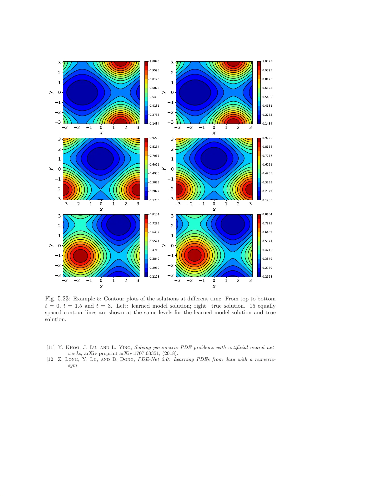
D A T A-DRIVEN DEEP LEARNING OF P AR TIAL DIFFERE N TIAL EQUA TIONS IN MODAL SP A C E KAILIANG WU AND DONGBIN X IU ∗ Abstract. W e presen t a fr amew ork f or reco vering/a pproximating unknown time-dependent partial differen tial equation (PDE) using its solution data. Instead of ident ifying the terms in the underlying PDE, we seek to approximate the evolut ion operator of the underlying PDE numerically . The evo lution op erator of the PDE , defined in infinite-dimensional space, maps the s ol ution fr om a current time to a future time and completely characte rizes the solution ev olution of the underlying unkno wn PDE. Our recov ery strategy relies on appro ximation of the ev olution op erator in a prop erly defined mo dal space, i.e., generalized F ourier space, i n order to r educe the problem to finite dimen- sions. The finite dimensional approximation is then accomplished by training a deep neural netw ork structure, whi c h is based on r esidual net work (ResNet), using the given data. Error analysis is pro- vided to illustrate the predictive accuracy of the pr op osed metho d. A set of examples of different t yp es of PDEs, including in viscid Burgers’ equat ion that develops discontin uit y in its solution, are presen ted to demonstrate the effectivene ss of the prop osed method. Key words. Deep neural netw ork, residual netw ork, gov erning equation discov ery , mo dal space 1. In tro duction. Recent ly there ha s b een an ong oing res earch effort to develop data-driven metho ds for discovering unknown physical laws. Earlier attempts such as [2, 30] used symbolic regressio n to select the pro p er physical laws and determine the underlying dynamica l sys tems. More r ecent efforts tend to cast the problem as an approximation problem. In this a pproach, the sought-after governing equation is treated as an unknown tar get function relating the data of the sta te v ar ia bles to their tempo ral deriv a tives. Metho ds along this line o f approach usually seek e x act recovery of the equations by using certain sparse approximation techniques (e.g., [32]) fro m a large set of dictionar ies; see, for example, [4]. St udies hav e b een conducted to dea l with noises in data [4 , 28, 9], c o rruptions in data [3 3], limited data [2 9], partial dif- ferential eq ua tions [25, 27], etc. V ariations of the a ppr oaches hav e been dev elop ed in conjunction with other metho ds such as mo del selectio n appro ach [14], Ko opman the- ory [3], Gaussian pr o cess r egress io n [20, 19], and expectatio n- maximization approach [15], to name a few. Methods using standard basis functions and without requir- ing exact recov ery w ere also developed for dynamical systems [38] and Hamiltonian systems [37]. There is a recent surge of in terest in developing metho ds using modern machine learning tec hniques, particularly deep neural netw orks . The studies include recovery of o rdinary differential equations (ODEs) [2 3, 17, 2 6] a nd par tial differential equa - tions (P DEs) [13, 21, 22, 18, 12, 3 1]. It was shown that residual net work (ResNet) is par ticularly suitable for equation re cov ery , in the sense that it can b e an exact int egra tor [17]. Neural netw orks hav e als o b een explored for other asp ects of sc ie n tific computing, including reduced or der mo deling [8, 1 6], solution of co nserv a tion laws [24, 36], multiphase flo w simulation [35], hig h-dimensional P DEs [6, 1 1], uncertaint y quantification [5, 34, 39, 10], etc. The fo cus of this pap er is o n the dev elopment of a genera l n umerical framework for a pproximating/learning unknown time-dep endent PDE. Even though the topic has b een explor ed in s e veral recent articles, cf., [13, 21, 22, 18, 1 2, 31], the e x ist- ∗ Departmen t of Mathematics, The Ohio Stat e Universit y , Columbus, OH 4 3210, USA. wu.3423@ osu.edu, xiu.16@osu.e du. F unding: This work was partially supported by AFOSR F A9550-18-1-0102. 1 ing studies are relatively limited, as they mostly fo c us on lea rning certain types of PDE or iden tifying the exact terms in the PDE from a (large) dictionar y of p ossi- ble terms. The sp ecific novelt y of this pap er is that the prop os e d method seeks to recov er/a pproximate the evolution op erator of the underlying unknown PDE and is applicable for g eneral class of P DEs. The evolution op erator completely characterizes the time evolution of the solution. Its recovery allows one to conduct predictio n of the underlying PDE and is effectively equiv alent to the recov ery o f the equation. This is an extensio n of the equation r ecov ery w ork fro m [17], where the flow map of the un- derlying unkno wn dyna mical sys tem is the goal of recov ery . Unlike the ODE s y stems considered in [17], PDE systems , which is the fo cus o f this pap er, ar e of infinite dimen- sion. In or der to cope with infinite dimension, our metho d first reduces the problem int o finite dimensio ns by utilizing a prop erly chosen mo dal space, i.e., g eneralized F ourie r space . The equa tion r ecov ery tas k is then trans formed in to recov ery of the generalized F our ier co efficients, whic h follow a finite dimensional dynamica l system. The approximation o f the finite dimensiona l evolution op erato r of the r educed sy stem is then carr ie d out b y using deep neural netw ork, particularly the residual netw ork (ResNet) which has been shown to b e particularly suitable for this task [17]. One of the adv an tages of the prop osed method is that, by focusing on evolution o p erator, it eliminates the need for time der iv atives da ta of the state v ar iables. Time deriv a tive data, often requir ed by many existing metho ds, a re difficult to a cquire in practice and susceptible to (additional) error s when co mputed numerically . Moreov er, the prop osed metho d can co p e with s olution data that are more sparsely or unevenly dis- tributed in time. Since the prop osed fra mework is rather g e neral, we present several examples of recov ering different types of PDEs. These include linear advection, linea r diffusion, viscous a nd inviscid nonlinear Burg ers’ equations. The inviscid Bur gers’ equation represents a rela tively c hallenging problem, as it develops sho ck o ver time. Our results show that the pr op osed metho d is able to accurately capture the evolution op erator us ing only smoo th data during tra ining. The rec o nstructed evolution op er - ator is then able to pro duce sho ck structure dev elop ed over time during prediction. Most o f our examples are in one dimensional physical space, as this allows us to easily and thoroughly examine the solutions and their numerical e rrors . Our la st example is the recovery of a tw o-dimensional advection-diffusion equa tio n. It demonstrates the applicability o f the metho d to m ultiple dimensional PDEs . This pap er is org anized a s follows. After the problem se tup in Sec tio n 2, we discuss evolution o pe r ator a nd its finite dimensiona l repr esentation in Section 3. The nu merica l approach for lear ning the evolution op erator is then presented in Section 4, a long with an e r ror analysis for the predictive accuracy . Numerica l examples ar e then presented in Section 5 to demons trate the pro per ties of the prop os ed approach. 2. Problem Setup. Let us consider a state v ar iable u ( x, t ), which is governed by an unkno wn autonomous time-dep endent PDE system      u t = L ( u ) , ( x, t ) ∈ Ω × R + , B ( u ) = 0 , ( x, t ) ∈ ∂ Ω × R + , u ( x, 0) = u 0 ( x ) , x ∈ ¯ Ω , (2.1) where t denotes the time, x is the spatial v ar ia ble, Ω is the physical domain, and L and B stand for the o p e r ators in the equations and b oundar y conditions, re sp e c tively . Our basic a ssumption is that the op erator L is unknown. In this pa pe r, we assume the b oundary co nditions ar e known and focus on learning the PDE in the interior of the domain. 2 W e a ssume da ta ab out the solution u ( x, t ) are av aila ble at certain time instances, lo osely called “ snapshots” hereafter. That is, we have data w ( x, t j ) = u ( x, t j ) + ǫ ( x, t j ) , j = 1 , . . . , S, (2.2) where S ≥ 1 is the total n umber of snapshots o f the solution field a nd ǫ ( x, t j ) stands for the no ises/err ors when the data a re acquired. (Certain reconstruction proce dure may b e inv olved in o rder to hav e the sna pshot data in the form of (2.2). This, howev er, is not the fo cus of this pap er.) Our goa l is to accurately reco nstruct the evolution/dynamics of the unknown gov erning equation (2.1) via the s napshot data (2 .2). O nce a n accur ate reco nstruction is achiev ed, it can b e used to provide pr edictions of the solutio n. 3. Finite Dime nsional Appro ximation. While many of the ex isting equation learning metho ds seek to dir ectly a ppr oximate or lear n the sp ecific form of the govern- ing equations, we ado pt a differen t framework, which s eeks to approximate evolution op erator of the underlying equations. Such an approach was presented and analyzed in [17] for recovery of O DEs. F or the P DE rec overy problem consider ed in this pap er, our first task is to reduce the proble m fro m infinite dimension to finite dimension. 3.1. Ev olution Op erator. Without specifying the form o f the gov erning e qua- tion, we lo os ely a ssume that for any fixed t ≥ 0, the so lution u ( x, t ) b elong s to a Hilber t space V , with the space norm denoted by k · k V . Moreov er, we assume the known b o undary conditions are linear, i.e., the b oundar y op er a tor B in (2.1) is linear. F or many co mmonly-used b ounda ry co nditions, e.g., Dir ichlet, Neuma nn, o r p erio dic bo undary conditions, etc., this assumption holds true. W e res trict our attention to autonomous P DEs. Co nsequently , there exists an evolution o p e rator E ∆ : V → V , E ∆ u ( · , t ) = u ( · , t + ∆) . (3.1) Note that only the time differ e nce, or time la g, ∆ is re lev ant, a s the time v ariable t ca n be ar bitr arily shifted. The e volution op erator co mpletely determines the solutio n ov er time. O nce it is accurately approximated, one can iter atively a pply the a pproximate evolution o p e rator to conduct pr ediction of the s ystem. 3.2. Finite Dimensi o nal Evolution Op erator. T o make the PDE learning problem tractable, we consider a finite dimens ional space V n ⊂ V . Let Φ ( x ) = ( φ 1 ( x ) , . . . , φ n ( x )) † , n ≥ 1 , (3.2) be a basis of V n and satisfy B ( φ j ) = 0, 1 ≤ j ≤ n , i.e., V n = span { φ j : B ( φ j ) = 0 , j = 1 , . . . , n } . (3.3) An approximation of u ( x, t ) from V n can b e written a s u n ( x, t ) = n X j =1 v j ( t ) φ j ( x ) = h v ( t ) , Φ ( x ) i , (3.4) where the last equality is written in vector notatio n a fter defining v = ( v 1 , . . . , v n ) † . Let P n : V → V n be a pro jection op era tor. F or any t , we define the pro jection of the exact solution as b u n ( x, t ) := P n u ( x, t ) = h b v ( t ) , Φ ( x ) i . (3.5) 3 T o approximate the (unknown) infinite dimensional evolution o per ator E ∆ in the finite dimensional space V n , we cons ider a finite dimensiona l evolution op erator E ∆ ,n , which e volv es an approximate so lutio n u n ∈ V n , i.e. E ∆ ,n : V n → V n , E ∆ ,n u n ( · , t ) = u n ( · , t + ∆) . (3.6) In pra c tice, one may cho o se any s uitable finite dimensiona l op era tor E ∆ ,n , as lo ng as it provides a go o d appr oximation to E ∆ , i.e., E ∆ ,n ≈ E ∆ . In this pape r , we mostly employ the follo wing finite dimensio nal evolution op er a tor e E ∆ ,n := P n E ∆ , (3.7) such that e E ∆ ,n v = P n E ∆ v , ∀ v ∈ V n . (3.8) (Note that if one choose s v = P n u , then this o p e r ator clo sely r esembles the evolution op erator o f sp ectral Ga lerkin metho d fo r solv ing an known PDE.) F or this sp ecific choice o f E ∆ ,n , w e have the following error b ound. Proposition 3. 1 . Assume the evolution op er ator E ∆ (3.1) of the underlying PDE is b ou n de d. L et t k = k ∆ , k = 0 , 1 , . . . , and let ε proj ( t k ) := k u ( · , t k ) − P n u ( · , t k ) k V b e the pr oje ction err or of the exact solution at t k . Consider the appr oximate evolution op er ator e E ∆ ,n define d in (3.7) and its c orr esp onding appr oximate solution: u n ( · , t k ) = e E ∆ ,n ( · , t k − 1 ) , k = 1 , 2 , . . . , u n ( · , 0) = b u n ( · , 0) . Then, the err or in the appr oximate solution satisfies k u n ( · , t k ) − u ( · , t k ) k V ≤ k X j =0 kP n E ∆ k k − j ε proj ( t j ) . (3.9) Pr o of . Le t e ( t k ) := k u n ( · , t k ) − b u ( · , t k ) k V . F or any k ≥ 1, we ha ve e ( t k ) = kE ∆ ,n u n ( · , t k − 1 ) − P n u ( · , t k ) k V = k P n E ∆ u n ( · , t k − 1 ) − P n E ∆ u ( · , t k − 1 ) k V ≤ k P n E ∆ u n ( · , t k − 1 ) − P n E ∆ b u n ( · , t k − 1 ) k V + kP n E ∆ b u n ( · , t k − 1 ) − P n E ∆ u ( · , t k − 1 ) k V ≤ k P n E ∆ k e ( t k − 1 ) + kP n E ∆ k ε proj ( t k − 1 ) . By recursively applying the ab ov e inequality a nd using e ( t 0 ) = 0, we obtain k u n ( · , t k ) − b u ( · , t k ) k V ≤ k − 1 X j =0 kP n E ∆ k k − j ε proj ( t j ) . The estimate (3.9) is further obtained by using k u n ( · , t k ) − u ( · , t k ) k V ≤ k u n ( · , t k ) − b u ( · , t k ) k V + k b u ( · , t k ) − u ( · , t k ) k V = e ( t k ) + ε proj ( t k ) . 4 W e now define a linear mapping Π : R n → V n , Π v = h v , Φ ( x ) i , v ∈ R n , (3.10) which is a bijective mapping whose in verse exists. Subsequently , Π : R n → V n is an isomorphism. This mapping defines a unique corre s po ndence betw een a solution in V n and its mo dal expa ns ion co efficients in R n . Proposition 3. 2. L et E ∆ ,n b e a finite dimensional evolution op er ator for u n ∈ V n , as define d in (3.6) , and v ∈ R n b e its c o efficient ve ctor as in (3.4) , then v fol lows an evolution op er ator M ∆ ,n : R n → R n , M ∆ ,n v ( t ) = v ( t + ∆) , (3.11) and M ∆ ,n = Π − 1 E ∆ ,n Π , (3.12) wher e Π is the line ar mapping define d in (3.10) . F u rthermor e, if E ∆ ,n is define d as in (3.7) , then M ∆ ,n = Π − 1 P n E ∆ Π =: f M ∆ ,n . (3.13) The pro o f is a tr ivial exercise o f substituting (3.10) in to (3.6). Therefore, w e have transfor med the learning of the infinite dimens io nal evolution op erator E ∆ (3.1) for the true solution u ∈ V to the learning of its finite dimensional approximation E ∆ ,n (3.6) for the a pproximate solution u n ∈ V n , which is equiv a lent to the lea rning of the evolution op era tor M ∆ ,n (3.11) for its expansion co efficient v ∈ R n . 4. Numerical Approac h. In this section, we discuss the de ta il of our P DE learning algor ithm. The genera l proc edure consists of the follo wing steps: • Cho o se a basis for the finite dimensio na l space V n (3.3) and a cor resp onding pro jection op erator (3.5). • Apply the pr o jection op era tion and pro ject the snapshot data (2.2) to V n (3.3) to obta in training data in mo da l space. • Cho o se an appro priate deep neural netw o rk structure to approximate the finite dimensional ev olution ope r ator M ∆ ,n (3.11) a nd conduct the netw ork training. • Conduct numerical pre diction of the system by adv ancing the lear ne d neural net work model for the evolution oper ator. W e remar k that this is a fa irly general pro cedure. One is certainly not confined to using neura l net work. Other approximation metho ds ca n also b e a pplied to mo del the evolution op erator. How ever, mo dern neural netw orks, along with their adv anced training algorithms, a re a ble to handle relatively high dimensional inputs. This feature makes them more suitable to PDE learning. 4.1. Basis Selection and Data Set Construction. The choice of basis func- tions is fair ly stra ightf orward – a n y ba sis suitable for spatial approximation of the solution da ta can b e used. The s e include piecewise polynomia ls, typically used in fi- nite differe nce or finite elements metho ds, or o rthogona l p olynomia ls used in sp ectra l metho ds, etc. The basis should also be sufficiently fine to r esolve the structure of the true solution. 5 Once the basis functions ar e s elected, one pro ceeds to employ a suitable pr o jection op erator P n : V → V n to represent the so lution in the finite dimensional form (3.5). This can be a ccomplished via pie c ewise interpo lation, a s commonly used in finite elements and finite difference methods, or orthog onal pro jection, which is often used in sp ectral metho ds. One of the k ey ingredien ts fo r lear ning the finite dimensiona l evolution op er ator M ∆ ,n (3.11) is to acquire mo dal vector data in pairs, whose co mpo nent s a r e separ ated by a time lag . That is, let J ≥ 1 b e the total num ber of solution data pairs. Then, we define the j - th data pair a s ( v j (0) , v j (∆ j )) , j = 1 , . . . , J, (4.1) where ∆ j > 0 is the time lag. Note again that for the autono mous systems c o nsidered in this pap er, the time difference ∆ j is the only r elav ent v ariable. Hereafter, w e w ill assume, without lo s s of generality , ∆ j = ∆ is a constant. 4.1.1. Data P airing via Snapshot Data Pro jection. When s o lution snap- shots a re av aila ble in the form of (2 .2), we first identify a nd create pairs of snapshots that a re separa ted b y the time la g ∆. That is, we seek to hav e the data arra nged in the following form ( u ( j ) ( · , t k j ) , u ( j ) ( · , t k j + ∆)) , j = 1 , . . . , J, (4.2) where J ≥ 1 is the tota l num ber of pairs. Note that some (or, even all) of the pairs may b e or iginated fr om the s ame “tra jectory”. Tha t is, they a re o bta ined fr om the origina l da ta snapshots (2.2) with the same initial condition. F o r more effectiv e equation recovery , it is strongly preferr ed that the data pair s ar e origina ted from different tr a jectories with a large num ber of different initia l conditions [17]. Once the snapshot data pairs ar e c o nstructed, we proc e e d to pro ject them o nt o the finite dimensiona l space V n by applying the pro jection oper ator (3.5). This then pro duces data pair s for the mo dal ex pa nsion co efficients (4.1), where v j (0) = Π − 1 P n u ( j ) ( · , t k j ) , v j (∆) = Π − 1 P n u ( j ) ( · , t k j + ∆) . Learning the finite dimensio nal e volution op erator is then c onducted in the mo dal space in sea rch for M ∆ ,n (3.11). This is a ccomplished by formally solving the following minimization pro blem: M ∆ ,n = argmin N ∆ : R n → R n 1 J J X j =1 kN ∆ v j (0) − v j (∆) k 2 2 . (4.3) This cor resp onds to finding the op era to r E ∆ ,n (3.6) by formally solving E ∆ ,n := arg min E ∆ : V n → V n 1 J J X j =1 k E ∆ b u ( j ) ( · , t k j ) − b u ( j ) ( · , t k j + ∆) k 2 V , (4.4) where b u ( j ) = P n u ( j ) . 4.1.2. Data P airing via Sampling in Mo dal Space. When data collection pro cedure is in a controlled environment, it is then p ossible to dir ectly sample in the mo dal space to generate the tra ining data pa irs. One example of such a case is when 6 the unknown PDE is controlled by a black-box simulation s oftw a re or a device. This would allow one to p ossibly generate arbitra ry “initial” conditions and then collect their sta tes at a later time. In this case, the tr aining data pairs (4.1) can b e genera ted as follows. • Sample J points { v j (0) } J j =1 ov er a domain D ⊂ R n , where D is a regio n in which o ne is interested in the so lution b ehavior. The sampling can b e conducted ra ndomly or by using o ther prop er sampling techniques. • F or each j = 1 , . . . , J , construct initial s olution u ( j ) ( x, 0) = Π v j (0) = h v j (0) , Φ ( x ) i . (4.5) Then, mar ch for ward in time for the time lag ∆, by using the underly- ing black-box simulation co de or device, and obtain the solutio n snapshots u ( j ) ( x, ∆). Conduct the pr o jection oper ation (3.5) to obtain v j (∆) = Π − 1 P n u ( j ) ( x, ∆) . (4.6) The mo dal expansion co efficients data gener ated in this manner then s a tisfy , for each j = 1 , . . . , J , v j (∆) = Π − 1 P n E ∆ u ( j ) ( x, 0) = Π − 1 P n E ∆ Π v j (0) = f M ∆ ,n v j (0) , where f M ∆ ,n is defined in (3.13) and co rresp onds to the finite dimensio nal ev olution op erator defined in (3.7). W e r emark that this pr o cedure also gener ates solution pairs alo ng the wa y , i.e, ( u ( j ) ( · , 0) , u ( j ) ( · , ∆)) , u ( j ) ( · , 0) ∈ V n , j = 1 , . . . , J. Note that here u ( j ) ( · , 0) ∈ V n due to (4.5 ) via the direct sampling in the mo da l space. These pairs are then different fro m those in (4.2), whose comp o nents are not necessarily in V n . 4.2. Neural Net w ork Mo deling of Evolution Op erator. Once the training data set (4 .1 ) b ecomes av ailable, one can pro cee d to learn the unknown governing equation. This is a chiev ed by learning the finite dimensional evolution o pe rator re- lating the solution coefficients in the data pairs. As shown in Pro po sition 3.2, finding the finite dimens io nal ev olution opera tor o f the unknown PDE (3.6) is eq uiv alent to find the evolution op erator (3 .12) for the mo dal expansion coe fficient v ectors. Sup- po se the solutio n co efficien t vectors formally follow an unknown autonomo us system, d v /dt = f ( v ), we then ha ve, by using mean-v alue theorem, v (∆) = M ∆ ,n ( v (0)) = v (0) + Z ∆ 0 f ( v ( t )) dt = v (0) + ∆ · f ( M τ ,n v (0)) , 0 ≤ τ ≤ ∆ , (4.7) where M ∆ ,n is the evolution ope rator defined in (3.12) a nd τ dep ends on ∆ and the form of the op era tor L in (2.1). F urthermo re, if M ∆ ,n takes the form of (3 .1 3), we 7 then hav e v (∆) = f M ∆ ,n ( v (0)) = Π − 1 P n E ∆ Π v (0) = Π − 1 P n E ∆ h v (0) , Φ ( x ) i = Π − 1 P n h v (0) , Φ ( x ) i + Z ∆ 0 L ( E t Π v (0)) dt ! = Π − 1 P n h v (0) , Φ ( x ) i + ∆ · Π − 1 P n L ( E τ Π v (0)) = v (0) + ∆ · Π − 1 P n L ( E τ Π v (0)) , 0 ≤ τ ≤ ∆ . (4.8) These relations s uggest that, when the time lag ∆ is small, it is natura l to ado pt the residue netw ork (ResNet) [7] to mo del the evolution op erator . This appro ach was pr esented and systematically s tudied in [17], for learning of unknown dynamical systems from data. The blo ck ResNet structur e for equation learning from [17] tak es the following form v (∆) = N ( v (0); Θ) , (4.9) where N denotes the nonlinear op erator defined by the underlying neural netw ork with parameter set Θ. F or blo ck ResNet with K ≥ 1 ResNet blo cks, the op erato r N =  I + N ( • ; Θ K − 1 )  ◦ · · · ◦  I + N ( • ; Θ 0 )  , with N is standard fully co nnected feedforward neur al netw ork, and Θ = { Θ i } 0 ≤ i ≤ K − 1 are the par ameters (weigh ts and biase s) in each Res Net blo ck. (See [17] for more details.) The parameters are determined by minimizing the loss function (4.3), i.e., L (Θ) = 1 J J X j =1 k N ( v j (0); Θ) − v j (∆) k 2 2 , (4.10) where k · k 2 denotes vector 2-nor m. Let Θ ∗ be the tra ined parameters, after satis fa ctory minimization of the los s function. A le arned mo del is then c o nstructed in the form of N ( · ; Θ ∗ ), which provides an appr oximation to the evolution op erato r (3.11), N ( · , Θ ∗ ) ≈ M ∆ ,n . (4.11) The trained net work mo del can then be use d to provide prediction o f the sys tem (2.1). F or an arbitr a ry initial condition u ( x, 0) ∈ V , we first conduct its pr o jection (3.5) and obta in b v (0) = Π − 1 P n u ( · , 0) , (4.12) where Π is the bijective mapping defined in (3.10). W e then iteratively apply the neural net work mo del (4 .1 1) to obtain approximate s olutions for the mo dal expansion co efficients a t time instances t k = k ∆, ( e v (0) = b v (0) , e v ( t k +1 ) = N ( e v ( t k ); Θ ∗ ) , k = 0 , . . . . (4.13) The predicted solutio n fields e u n ( x, t k ) are then obtained b y e u n ( x, t k ) = Π e v ( t k ) = h e v ( t k ) , Φ ( x ) i , k = 1 , . . . . (4.14) 8 4.3. Error Analysis. W e now derive an erro r b ound for the predicted solution (4.14) of our neural netw ork mode l, when the finite dimensio nal ev olution op erator (3.13) is the case, i.e., M ∆ ,n = f M ∆ ,n = Π − 1 P n E ∆ Π. F o r notational conv enience, w e assume that the ba s is functions { φ j ( x ) } n j =1 of V n are orthonorma l. (Note that non- orthogo nal basis can always b e orthogonalize d via Gram-Schmidt pro cedure.) Then, the bijective mapping Π : R n → V n defined in (3 .10) is an iso metric isomorphis m and satisfies k Π v k V = k v k 2 , v ∈ R n . Also, s ince it is well known that neural netw orks are universal a pproximator for a general class o f functions, we ass ume that the tr a ining erro r in (4.11) is b ounded. W e then state the following result. Theorem 4.1. Assum e the evolution op er ator E ∆ (3.1) of the underlying PDE is b oun de d. Also, assume the t r aine d neur al net work mo del N = N ( · , Θ ∗ ) is b ounde d, and its appr oximation err or (4.11) is b oun de d and denote ε DNN := k N − Π − 1 P n E ∆ Π k < + ∞ . L et t k = k ∆ , k = 0 , 1 , . . . , and let ε proj ( t k ) := k u ( x, t k ) − P n u ( x, t k ) k V b e the pr oje ction err or of the exact solution at t k . Then the following err or b ounds hold : k e v ( t k ) − b v ( t k ) k 2 ≤ k − 1 X j =0 k N k k − 1 − j  ε DNN k b v ( t j ) k 2 + ε proj ( t j ) kP n E ∆ k  , (4.15) wher e b v = Π − 1 b u is the mo dal exp ansion c o efficient ve ctor of t he pr oje cte d exact solu- tion (3.5) and e v is the c o efficient ve ctor pr e dicte d by t he neur al network mo del (4.1 3) , and k e u n ( · , t k ) − u ( · , t k ) k V ≤ ε proj ( t k ) + k − 1 X j =0 k N k k − 1 − j  ε DNN k b v ( t j ) k 2 + ε proj ( t j ) kP n E ∆ k  , (4.16) wher e e u is the solution state pr e dicte d by the t r aine d neur al n et work mo del (4.14) . Pr o of . Le t e ( t k ) := k e v ( t k ) − b v ( t k ) k 2 . Note that, for k = 1 , . . . , b v ( t k ) = Π − 1 b u n ( · , t k ) = Π − 1 P n u ( · , t k ) = Π − 1 P n E ∆ u ( · , t k − 1 ) . W e then ha ve e ( t k ) = k e v ( t k ) − Π − 1 P n E ∆ u ( · , t k − 1 ) k 2 ≤ k e v ( t k ) − Π − 1 P n E ∆ b u n ( · , t k − 1 ) k 2 + k Π − 1 P n E ∆ b u n ( · , t k − 1 ) − Π − 1 P n E ∆ u ( · , t k − 1 ) k 2 = k N ( e v ( t k − 1 ); Θ ∗ ) − Π − 1 P n E ∆ Π v ( t k − 1 ) k 2 + kP n E ∆ b u n ( · , t k − 1 ) − P n E ∆ u ( · , t k − 1 ) k V ≤ k N ( e v ( t k − 1 ); Θ ∗ ) − N ( b v ( t k − 1 ); Θ ∗ ) k 2 + k N ( b v ( t k − 1 ); Θ ∗ ) − Π − 1 P n E ∆ Π b v ( t k − 1 ) k 2 + kP n E ∆ kk b u n ( · , t k − 1 ) − u ( · , t k − 1 ) k V ≤ k N k e ( t k − 1 ) + ε DNN k b v ( t k − 1 ) k 2 + kP n E ∆ k ε proj ( t k − 1 ) . 9 By recur sively a pplying the ab ov e inequality and using e ( t 0 ) = 0 , we obtain (4.15). The pro o f is then complete by using k e u n ( · , t k ) − u ( · , t k ) k V ≤ k e u n ( · , t k ) − P n u ( · , t k ) k V + kP n u ( · , t k ) − u ( · , t k ) k V = k e v ( t k ) − b v ( t k ) k 2 + ε proj ( t k ) = e ( t k ) + ε proj ( t k ) . Theorem 4 .1 indicates that the prediction er ror of the netw ork mo del is a ffected by the approximation err or of the neural netw ork and the pro jection er ror, which is determined by the approximation s pace V n and the r egularity o f the solution. 5. Numerical E xamples. In this section, we present numerical examples to verify the prop er ties of the prop osed metho d. F or b enchmarking purpo se, the true gov erning PDEs a re k nown in all of them exa mples. Howev er, we use the true g ov ern- ing equatio ns only to generate training da ta, particula rly by following the pro cedure in Section 4.1.2. O ur prop osed lea rning metho d is then applied to these synthetic data and pro duces a trained neura l netw ok mo del for the underlying PDE. W e will then use the neur a l net work mo del to conduct numerical predictions of the so lution and c o mpare them a gainst the r eference so lution pr o duced by the governing equa - tions. Numerical er rors will b e r epo rted, in term of relative error s b etw een the neur a l net work prediction solutions and the reference solutions. The gov erning equatio ns co nsidered in this section include: linear advection equa- tion, linear diffusion equa tion, nonlinea r vis c ous Burger s’ equation, nonlinear inviscid Burgers ’ equation, the last o f which pro duces sho cks. W e primar ily fo cus o n one dimension in physical space with noiseless data , in o rder to conduct detailed and thorough examination o f the solution b ehavior. Data noises are introduced in one ex- ample to demons tr ate the applica bility of the method. A t wo-dimensional advection- diffusion problem is also presented demonstr a te the a pplicability of the metho d to m ultiple dimensio ns. In a ll ex amples, w e employ g lobal o rthogonal p oly nomials a s the basis functions to define the finite dimens io nal space for training. F or b enchmarking purp ose, all training data ar e generated in mo dal spa ce, as descr ibe d in Section 4.1 .2. W e also rather arbitrarily impose a decay condition in certa in examples to ensur e the higher mo des are smaller, co mpared to the low er mo des . This effectively p oses a smo o thness condition on the training data. All of our net work models a re trained via minimizing the loss function (4.3) and by using the op en-sour c e T enso r flow libr ary [1]. The training data set is divided into mini-batches of s iz e 10 , and the learning r ate is taken as 0 . 0 01. The netw ork eights are initialized randomly from Gaussian distributions and biases are initialized to zeros. Upo n success ful training , the neural netw ork mo dels ar e then marched forward in time with the ∆ time step, as in (4 .13). The results, la b elled as “pr ediction”, are compared against the reference s olutions, labelled as “exact”, of the true under lying gov erning equations. 5.1. Example 1: Advection Equation. W e fir s t consider a one-dimensiona l advection equation with p erio dic b oundary co ndition: ( u t + u x = 0 , ( x, t ) ∈ (0 , 2 π ) ∈ R + , u (0 , t ) = u (2 π , t ) , t ∈ R + . (5.1) 10 The finite dimensional a ppr oximation space is s et as V n = s pa n { e ikx , k ≤ 3 } , which implies n = 7. The time la g ∆ is taken as 0 .1. The domain D in the mo dal space is fixed as [ − 0 . 8 , 0 . 8] for k ≤ 1 and [ − 0 . 2 , 0 . 2 ] fo r k = 2, and [ − 0 . 03 , 0 . 03 ] for k = 3. By using unifor m distribution, we genera te 80 , 000 training data in the modal space. F or neural netw ork mo deling, we employ the blo ck ResNet structure with t wo blo cks ( K = 2), each of which contains 3 hidden lay ers of equal width of 30 neurons. The loss function training history is shown in Fig. 5.1, w her e the netw ork is tra ined for up to 2 , 000 epo chs. Conv ergence can b e achiev ed after ab out 200 ep o chs. T o v alida te the model, we employ an initial condition u 0 ( x ) = 1 2 exp(sin( x )) and co nduct simulations using the trained mode l, in the for m of (4.1 2)–(4.14), for up to t = 20. Note that this particular initial c o ndition, a lbe it smo o th, is fairly repr e s ent ative, as it is not in the appr oximation s pa ce V n . In Fig. 5.2, the solution prediction of the trained mo del is plotted at differen t time instances, along with the true solution for compariso n. The relative erro r in the predicted solution is shown in Fig. 5.3. W e observe that the netw ork mo del pro duces ac c urate prediction r esults for time up to t = 20. The erro r grows ov er time. This is consistent with the err or estimate fro m Theorem 4.1 and is exp ected fr om any numerical time int egr a tor. T o further ex amine the so lution prop er t y , we also plot in Fig. 5.4 the evolution of the learned expansio n co efficients ˆ v j , 1 ≤ j ≤ 7. F or reference purp ose, the optimal co e fficient s obtained by the L 2 B (Ω) orthogo nal pro jection o f the true so lution o nt o V n are also plotted. W e observe g o o d agreement b etw een the t w o solutions. 0 2 5 0 5 0 0 7 5 0 1 0 0 0 1 2 5 0 1 5 0 0 1 7 5 0 2 0 0 0 e p o c h 1 0 − 7 1 0 − 6 1 0 − 5 1 0 − 4 1 0 − 3 1 0 − 2 1 0 − 1 e r r o r Fig. 5.1: Example 1: T raining loss history . 5.2. Example 2: Diffusion Equation. W e now consider the following diffu- sion equation with Dir ichlet b ounda ry condition: ( u t = σ u xx , ( x, t ) ∈ (0 , π ) × R + , u (0 , t ) = u ( π , t ) = 0 , t ∈ R + . (5.2) The finite dimensional approximation s pace is chosen as V n = spa n { sin( j x ) , 1 ≤ j ≤ 5 } , where n = 5. (The symmetry o f the pr oblem allows this simplified choice to facilitate the computation and compar ison.) The time lag ∆ is ta ken as 0.1. The domain D in the mo da l space is taken as [ − 1 , 1 ] × [ − 0 . 5 , 0 . 5] × [ − 0 . 2 , 0 . 2] × [ − 0 . 05 , 0 . 05] × [ − 0 . 01 , 0 . 01], from which we sa mple 3 0 , 00 0 training data. In this 11 0 1 2 3 4 5 6 x 0 . 2 0 . 4 0 . 6 0 . 8 1 . 0 1 . 2 1 . 4 u p r e d i c t i o n e x a c t 0 1 2 3 4 5 6 x 0 . 2 0 . 4 0 . 6 0 . 8 1 . 0 1 . 2 1 . 4 u p r e d i c t i o n e x a c t 0 1 2 3 4 5 6 x 0 . 2 0 . 4 0 . 6 0 . 8 1 . 0 1 . 2 1 . 4 u p r e d i c t i o n e x a c t 0 1 2 3 4 5 6 x 0 . 2 0 . 4 0 . 6 0 . 8 1 . 0 1 . 2 1 . 4 u p r e d i c t i o n e x a c t 0 1 2 3 4 5 6 x 0 . 2 0 . 4 0 . 6 0 . 8 1 . 0 1 . 2 1 . 4 u p r e d i c t i o n e x a c t 0 1 2 3 4 5 6 x 0 . 2 0 . 4 0 . 6 0 . 8 1 . 0 1 . 2 1 . 4 u p r e d i c t i o n e x a c t Fig. 5.2: Example 1: Comparison of the t ru e solution and the learned mo del solution at different time. T op-left: t = 1; top-right: t = 2; middle-left: t = 3; middle-right: t = 4; b ottom-left: t = 10; b ottom-righ t: t = 20. example, we employ a sing le -blo ck Res Net metho d ( K = 1) c o ntaining 3 hidden lay ers of equal width of 30 neurons . The training of the netw ork mo del is conducted for up to 50 0 ep o chs, where satisfactor y co n vergence is esta blished, as shown in Fig. 5.5. F o r v alida tio n and a ccuracy tes t, we conduct numerical predictions of the tr a ined netw ork mo del using initial condition u 0 ( x ) = x π  5 − 4 x π − 7  x π  2 + 6  x π  3  , for up to time t = 3. Fig. 5.6 shows the solution predicted by the trained netw ork mo del, along with the exa c t solution of the true equation (5.2). It can b e seen that the predicted solution agr ees w ell with the exact solution. The relative error in the nu merica l prediction is shown in Fig. 5.7, in term of l 2 -norm. Finally , the e volution of the expansion coefficients is also sho wn given in Fig. 5.8. W e o bserve that they agree 12 0 . 0 2 . 5 5 . 0 7 . 5 1 0 . 0 1 2 . 5 1 5 . 0 1 7 . 5 2 0 . 0 t 1 0 − 3 1 0 − 2 1 0 − 1 p r e d i c t i o n e r r o r Fig. 5.3: Example 1: The evol ution of the relative error in the p rediction in l 2 -norm. well with the o ptimal coefficients obta ined by pr o jecting the exact so lution o nt o the linear space V n . W e now consider the ca se of no isy data. All training da ta a r e then pe rturb ed by a m ultiplicative factor (1 + ǫ ), where ǫ ∼ [ − η , η ] follows uniform distribution. W e consider tw o cases of η = 0 . 02 and η = 0 . 05, which respec tively corres p o nd to ± 2 % and ± 5% relative noises in all data. In Fig. 5.9, the numerical solutions pro duced b y the neural net wrok mode ls ar e presented, a fter net work training of 500 ep o chs, along with the exact solution. W e o bserve that the pr edictions of the netw o rk mo del ar e fairly r obust against data noise. At higher level noises in data, the predictive results contain r elatively lar g er n umerical er rors, as exp ected. 5.3. Example 3: Vis cous Burge rs’ Equation. W e no w consider the viscous Burgers ’ equation with Diric hlet b oundar y condition: ( u t +  u 2 2  x = σ u xx , ( x, t ) ∈ ( − π , π ) × R + , u ( − π , t ) = u ( π , t ) = 0 , t ∈ R + . (5.3) W e first consider a mo de s tly large v iscosity σ = 0 . 5. T he a pproximation space is chosen as V n = span { sin( j x ) , 1 ≤ j ≤ 5 } with n = 5. The time lag ∆ is fixed at ∆ = 0 . 05. The domain D in the mo dal spa ce is c hosen as [ − 1 . 5 , 1 . 5 ] × [ − 0 . 2 , 0 . 2] × [ − 0 . 05 , 0 . 05] × [ − 0 . 0 1 , 0 . 01 ] × [ − 0 . 002 , 0 . 002], from which 10 0 , 00 0 training data are generated. The block ResNet method with tw o blo cks ( K = 2) is used, where each blo ck contains 3 hidden lay ers o f equal width of 30 neurons. Up on training the netw ork mo del sa tisfactorily (see Fig. 5.10 fo r the training loss histo ry), we v alidate the tra ined mo del for the initial condition u 0 ( x ) = − sin ( x ) , for time up to t = 2. In Fig. 5.11, we compare the predicted s olution aga inst the exact solution at different time. The err o r of the prediction is co mputed and display ed in Fig. 5.12. W e observe that the net work mo de l pro duces accurate prediction r esults. The lear ned expa nsion co efficients are shown in Fig. 5.1 3 a nd ag r ee well with the optimal co efficients given by orthogona l pro jection of the exa ct solution. W e then consider a smaller viscosity σ = 0 . 1. The approximation space is chosen to b e relatively lar ger as V n = span { sin( j x ) , 1 ≤ j ≤ 9 } with n = 9. The time 13 0 . 0 2 . 5 5 . 0 7 . 5 1 0 . 0 1 2 . 5 1 5 . 0 1 7 . 5 2 0 . 0 t 0 . 6 2 0 0 . 6 2 5 0 . 6 3 0 0 . 6 3 5 0 . 6 4 0 0 . 6 4 5 0 . 6 5 0  v 1 o p t i ma l p r e d i c t i o n 0 . 0 2 . 5 5 . 0 7 . 5 1 0 . 0 1 2 . 5 1 5 . 0 1 7 . 5 2 0 . 0 t − 0 . 6 − 0 . 4 − 0 . 2 0 . 0 0 . 2 0 . 4 0 . 6  v 2 o p t i m a l p r e d i c t i o n 0 . 0 2 . 5 5 . 0 7 . 5 1 0 . 0 1 2 . 5 1 5 . 0 1 7 . 5 2 0 . 0 t − 0 . 6 − 0 . 4 − 0 . 2 0 . 0 0 . 2 0 . 4 0 . 6  v 3 o p t i m a l p r e d i c t i o n 0 . 0 2 . 5 5 . 0 7 . 5 1 0 . 0 1 2 . 5 1 5 . 0 1 7 . 5 2 0 . 0 t − 0 . 1 5 − 0 . 1 0 − 0 . 0 5 0 . 0 0 0 . 0 5 0 . 1 0 0 . 1 5  v 4 o p t i ma l p r e d i c ti o n 0 . 0 2 . 5 5 . 0 7 . 5 1 0 . 0 1 2 . 5 1 5 . 0 1 7 . 5 2 0 . 0 t − 0 . 1 5 − 0 . 1 0 − 0 . 0 5 0 . 0 0 0 . 0 5 0 . 1 0 0 . 1 5  v 5 o p ti m a l p r e d i c ti o n 0 . 0 2 . 5 5 . 0 7 . 5 1 0 . 0 1 2 . 5 1 5 . 0 1 7 . 5 2 0 . 0 t − 0 . 0 2 − 0 . 0 1 0 . 0 0 0 . 0 1 0 . 0 2  v 6 o p ti m a l p r e d i c ti o n 0 . 0 2 . 5 5 . 0 7 . 5 1 0 . 0 1 2 . 5 1 5 . 0 1 7 . 5 2 0 . 0 t − 0 . 0 2 − 0 . 0 1 0 . 0 0 0 . 0 1 0 . 0 2  v 7 o p t i m a l p r e d i c t i o n Fig. 5.4: Example 1: Evolution of the expansion coefficients for the learned mo del solution and th e pro jectio n of the true solution. lag ∆ is taken as 0.05. The domain D in the mo dal space is taken a s [ − 1 . 5 , 1 . 5] × [ − 0 . 5 , 0 . 5] × [ − 0 . 2 , 0 . 2] 2 × [ − 0 . 1 , 0 . 1] 2 × [ − 0 . 05 , 0 . 05] 2 × [ − 0 . 02 , 0 . 02], from which we sample 500 , 000 training data. In this example, w e use the four-blo ck ResNet metho d ( K = 4 ) with each blo ck co n taining 3 hidden layers of eq ua l width of 30 neuro ns. The net work mo del is trained for up to 2,000 ep o chs, and training los s histor y is shown in 14 0 1 0 0 2 0 0 3 0 0 4 0 0 5 0 0 e p o c h 1 0 − 9 1 0 − 8 1 0 − 7 1 0 − 6 1 0 − 5 1 0 − 4 1 0 − 3 1 0 − 2 e r r o r Fig. 5.5: Example 2: T raining loss history . 0 . 0 0 . 5 1 . 0 1 . 5 2 . 0 2 . 5 3 . 0 x 0 . 0 0 . 2 0 . 4 0 . 6 0 . 8 1 . 0 u p r e d i c t i o n e x a c t 0 . 0 0 . 5 1 . 0 1 . 5 2 . 0 2 . 5 3 . 0 x 0 . 0 0 . 2 0 . 4 0 . 6 0 . 8 1 . 0 u p r e d i c t i o n e x a c t 0 . 0 0 . 5 1 . 0 1 . 5 2 . 0 2 . 5 3 . 0 x 0 . 0 0 . 2 0 . 4 0 . 6 0 . 8 1 . 0 u p r e d i c t i o n e x a c t 0 . 0 0 . 5 1 . 0 1 . 5 2 . 0 2 . 5 3 . 0 x 0 . 0 0 . 2 0 . 4 0 . 6 0 . 8 1 . 0 u p r e d i c t i o n e x a c t Fig. 5.6: Example 2: Comparison of the t ru e solution and the learned mo del solution at different time. T op-left: t = 0; top- right: t = 1; bottom-left: t = 2; b ottom-right: t = 3. Fig. 5.1 4. T hen w e v a lidate the trained model for the initial condition u 0 ( x ) = − sin ( x ) . In Fig. 5.15, w e present the prediction results generated by the trained netw o rk, for time up to t = 2. One can see that the predicted solutions a re very close to the exact ones, This can also b e seen in the r elative error of the pr ediction from Fig. 5.16. W e note that a t time t = 2 the exact s olution develops a relatively sha rp (alb eit s till smo oth) transition lay er at this relatively low vis o city . The n umerical solution star ts 15 0 . 0 0 . 5 1 . 0 1 . 5 2 . 0 2 . 5 3 . 0 t 1 0 − 4 1 0 − 3 1 0 − 2 p r e d i c t i o n e r r o r Fig. 5.7: Example 2: The evol ution of the relative error in the p rediction in l 2 -norm. 0 .0 0 . 5 1 .0 1 .5 2 . 0 2 .5 3 . 0 t 0 .7 5 0 .8 0 0 .8 5 0 .9 0 0 .9 5  v 1 o p ti m a l p r e d i c ti o n 0 . 0 0 . 5 1 . 0 1 . 5 2 . 0 2 . 5 3 . 0 t 0 . 0 7 5 0 . 1 0 0 0 . 1 2 5 0 . 1 5 0 0 . 1 7 5 0 . 2 0 0 0 . 2 2 5 0 . 2 5 0  v 2 o p ti m a l p r e d i c ti o n 0 . 0 0 . 5 1 . 0 1 . 5 2 . 0 2 . 5 3 . 0 t − 0 . 0 2 5 − 0 . 0 2 0 − 0 . 0 1 5 − 0 . 0 1 0 − 0 . 0 0 5  v 3 o p ti m a l p r e d i c ti o n 0 . 0 0 . 5 1 . 0 1 . 5 2 . 0 2 . 5 3 . 0 t 0 . 0 0 0 0 . 0 0 5 0 . 0 1 0 0 . 0 1 5 0 . 0 2 0 0 . 0 2 5 0 . 0 3 0  v 4 o p ti m a l p r e d i c ti o n 0 .0 0 . 5 1 . 0 1 . 5 2 . 0 2 . 5 3 . 0 t − 0 . 0 0 6 − 0 . 0 0 5 − 0 . 0 0 4 − 0 . 0 0 3 − 0 . 0 0 2 − 0 . 0 0 1 0 . 0 0 0  v 5 o p ti m a l p re d i c ti o n Fig. 5.8: Example 2: Evolution of the expansion co efficients for the learn mod el and the pro jection of the true solution. to exhibit Gibbs’ type small os c illations. This is a rather common feature for global t yp e approximation and is not unexp ected. Comparison b e tween the lea rned a nd optimal expansion co e fficie nts is also shown in Fig. 5.17. 5.4. Example 4: In viscid Burgers’ Equation. W e now consider the inviscid Burgers ’ equation with Diric hlet b oundar y condition: ( u t +  u 2 2  x = 0 , ( x, t ) ∈ ( − π , π ) × R + , u ( − π , t ) = u ( π , t ) = 0 , t ∈ R + . (5.4) This represents a challenging pro blem, as the nonlinear hyper b o lic nature o f this equation can pro duce s ho c ks ov er time even if the initial solution is smo o th. The approximation spac e is chosen as V n = spa n { sin( j x ) , 1 ≤ j ≤ 9 } with n = 9. The time lag ∆ is taken as 0 . 05. The domain D in the mo dal spa ce is taken a s [ − 1 . 1 , 1 . 1] × [ − 0 . 5 , 0 . 5] × [ − 0 . 3 × 0 . 3] 7 , from which we sample 1 , 000 , 00 0 training data. W e remark that b y sampling in this manner , all of our training data are s mo oth. In 16 0 . 0 0 . 5 1 . 0 1 . 5 2 . 0 2 . 5 3 . 0 x 0 . 0 0 . 2 0 . 4 0 . 6 0 . 8 1 . 0 u p r e d i c t i o n e x a c t 0 . 0 0 . 5 1 . 0 1 . 5 2 . 0 2 . 5 3 . 0 x 0 . 0 0 . 2 0 . 4 0 . 6 0 . 8 1 . 0 u p r e d i c t i o n e x a c t 0 . 0 0 . 5 1 . 0 1 . 5 2 . 0 2 . 5 3 . 0 x 0 . 0 0 . 2 0 . 4 0 . 6 0 . 8 1 . 0 u p r e d i c t i o n e x a c t 0 . 0 0 . 5 1 . 0 1 . 5 2 . 0 2 . 5 3 . 0 x 0 . 0 0 . 2 0 . 4 0 . 6 0 . 8 1 . 0 u p r e d i c t i o n e x a c t 0 . 0 0 . 5 1 . 0 1 . 5 2 . 0 2 . 5 3 . 0 x 0 . 0 0 . 2 0 . 4 0 . 6 0 . 8 1 . 0 u p r e d i c t i o n e x a c t 0 . 0 0 . 5 1 . 0 1 . 5 2 . 0 2 . 5 3 . 0 x 0 . 0 0 . 2 0 . 4 0 . 6 0 . 8 1 . 0 u p r e d i c t i o n e x a c t Fig. 5.9 : Example 2: The solution at d ifferen t time predicted b y the neural netw ork model trained with n oisy data. Left: 2% noise; righ t: 5% noise. F rom top to bottom: solutions at t = 1, t = 2 and t = 3, respectively . this example, we use the blo ck ResNet metho d with K = 4 blo cks, each of which contains 3 hidden lay ers of equal width of 30. The net work training is conducted for up to 2 , 000 ep o chs, when it w as deemed satisfactory , as shown in the loss histor y in Fig. 5.1 8. F or v alidation, we conduct system prediction using initial condition u 0 ( x ) = − sin ( x ) , for time up to t = 2. Although the initial condition is smo o th, the exact solution will start to develop sho ck at t = 1. The prediction results gener ated by our net work mo del ar e shown in Fig. 5 .1 9, along with the exact so lutio n, a nd the Galerkin solution of the B ur gers’ e q uation using the same linea r space V n . Due to the discont inuit y in the so lutio n, Gibbs type oscillations app ear in the predicted solutions. This is not unexp ected, as the b est representation of a dis contin uous function using the linear subspace V n will natura lly 17 0 2 5 0 5 0 0 7 5 0 1 0 0 0 1 2 5 0 1 5 0 0 1 7 5 0 2 0 0 0 e p o c h 1 0 − 8 1 0 − 7 1 0 − 6 1 0 − 5 1 0 − 4 1 0 − 3 1 0 − 2 e r r o r Fig. 5.10: Ex ample 3: T raining loss history . − 3 − 2 − 1 0 1 2 3 x − 1 . 0 0 − 0 . 7 5 − 0 . 5 0 − 0 . 2 5 0 . 0 0 0 . 2 5 0 . 5 0 0 . 7 5 1 . 0 0 u p r e d i c t i o n e x a c t − 3 − 2 − 1 0 1 2 3 x − 1 . 0 0 − 0 . 7 5 − 0 . 5 0 − 0 . 2 5 0 . 0 0 0 . 2 5 0 . 5 0 0 . 7 5 1 . 0 0 u p r e d i c t i o n e x a c t − 3 − 2 − 1 0 1 2 3 x − 1 . 0 0 − 0 . 7 5 − 0 . 5 0 − 0 . 2 5 0 . 0 0 0 . 2 5 0 . 5 0 0 . 7 5 1 . 0 0 u p r e d i c t i o n e x a c t − 3 − 2 − 1 0 1 2 3 x − 1 . 0 0 − 0 . 7 5 − 0 . 5 0 − 0 . 2 5 0 . 0 0 0 . 2 5 0 . 5 0 0 . 7 5 1 . 0 0 u p r e d i c t i o n e x a c t Fig. 5.11 : Examp le 3: Comparison of th e true solution, the learned mo del solution and the solution by Galerkin metho d at different time. T op-left: t = 0 . 5; t op-right: t = 1; b ottom-left: t = 1 . 5; b ottom- right: t = 2. pro duce oscilla tions, unless special tr eatment such as filtering is utilized (whic h is not pursued in this work). The Galer kin so lution of the eq uation (5.4) exhibits the similar Gibbs’ oscillations for precisely the same reason. W e r emark that it can be seen that our neural netw ork pr ediction is visibly b etter than the Galer kin so lution. While the netw ork pr ediction is en tirely da ta driven and do e s not requir e knowledge of the equation, the Galerkin s olution is attainable o nly after knowing the pr ecise form of the gov erning equation. In Fig. 5.2 1, we plot the evolution of the ex pansion co efficients in the mo dal space o btained by the neural netw ork mode l prediction, Galer kin solution 18 0 . 0 0 0 . 2 5 0 . 5 0 0 . 7 5 1 . 0 0 1 . 2 5 1 . 5 0 1 . 7 5 2 . 0 0 t 1 0 − 4 1 0 − 3 1 0 − 2 p r e d i c t i o n e r r o r Fig. 5.12: Ex ample 3: The ev olution of the relative errors in the prediction in l 2 -norm. 0 . 0 0 0 . 2 5 0 . 5 0 0 . 7 5 1 .0 0 1 . 2 5 1 . 5 0 1 . 7 5 2 . 0 0 t − 1 .0 − 0 .9 − 0 .8 − 0 .7 − 0 .6 − 0 .5 − 0 .4  v 1 o p ti m a l p r e d i c ti o n 0 . 0 0 0 . 2 5 0 . 5 0 0 .7 5 1 . 0 0 1 . 2 5 1 .5 0 1 . 7 5 2 . 0 0 t −0 . 1 2 −0 . 1 0 −0 . 0 8 −0 . 0 6 −0 . 0 4 −0 . 0 2 0 . 0 0  v 2 o p t i ma l p r e d i c t i o n 0 . 0 0 0 . 2 5 0 . 5 0 0 . 7 5 1 . 0 0 1 . 2 5 1 . 5 0 1 . 7 5 2 . 0 0 t − 0 . 0 2 5 − 0 . 0 2 0 − 0 . 0 1 5 − 0 . 0 1 0 − 0 . 0 0 5 0 . 0 0 0  v 3 o p ti m a l p r e d i c ti o n 0 . 0 0 0 . 2 5 0 . 5 0 0 . 7 5 1 . 0 0 1 . 2 5 1 . 5 0 1 . 7 5 2 . 0 0 t − 0 . 0 0 5 − 0 . 0 0 4 − 0 . 0 0 3 − 0 . 0 0 2 − 0 . 0 0 1 0 . 0 0 0  v 4 o p ti m a l p re d i c ti o n 0 . 0 0 0 . 2 5 0 . 5 0 0 . 7 5 1 . 0 0 1 . 2 5 1 . 5 0 1 . 7 5 2 . 0 0 t −0 . 0 0 1 2 −0 . 0 0 1 0 −0 . 0 0 0 8 −0 . 0 0 0 6 −0 . 0 0 0 4 −0 . 0 0 0 2 0 . 0 0 0 0  v 5 o p ti m a l p re d i c t i o n Fig. 5.1 3: Example 3: Evol ution of th e expan sion co efficients for the learned mo del and t h e pro jection of the true solution. 0 2 5 0 5 0 0 7 5 0 1 0 0 0 1 2 5 0 1 5 0 0 1 7 5 0 2 0 0 0 e p o c h 1 0 − 7 1 0 − 6 1 0 − 5 1 0 − 4 1 0 − 3 1 0 − 2 1 0 − 1 e r r o r Fig. 5.14: Ex ample 3: T raining loss history . 19 − 3 − 2 − 1 0 1 2 3 x − 1 . 0 0 − 0 . 7 5 − 0 . 5 0 − 0 . 2 5 0 . 0 0 0 . 2 5 0 . 5 0 0 . 7 5 1 . 0 0 u p r e d i c t i o n e x a c t − 3 − 2 − 1 0 1 2 3 x − 1 . 0 0 − 0 . 7 5 − 0 . 5 0 − 0 . 2 5 0 . 0 0 0 . 2 5 0 . 5 0 0 . 7 5 1 . 0 0 u p r e d i c t i o n e x a c t − 3 − 2 − 1 0 1 2 3 x − 1 . 0 0 − 0 . 7 5 − 0 . 5 0 − 0 . 2 5 0 . 0 0 0 . 2 5 0 . 5 0 0 . 7 5 1 . 0 0 u p r e d i c t i o n e x a c t − 3 − 2 − 1 0 1 2 3 x − 1 . 0 0 − 0 . 7 5 − 0 . 5 0 − 0 . 2 5 0 . 0 0 0 . 2 5 0 . 5 0 0 . 7 5 1 . 0 0 u p r e d i c t i o n e x a c t Fig. 5.15 : Examp le 3: Comparison of th e true solution, the learned mo del solution and the solution by Galerkin metho d at different time. T op-left: t = 0 . 5; t op-right: t = 1; b ottom-left: t = 1 . 5; b ottom- right: t = 2. 0 . 0 0 0 . 2 5 0 . 5 0 0 . 7 5 1 . 0 0 1 . 2 5 1 . 5 0 1 . 7 5 2 . 0 0 t 1 0 − 4 1 0 − 3 1 0 − 2 1 0 − 1 p r e d i c t i o n e r r o r Fig. 5.1 6: Ex ample 3: The ev olution of the relative error in prediction in l 2 -norm. of the Burge rs’ eq ua tion, and orthog onal pro jection o f the exact solution (denoted a s “optimal”), the last of whic h serves as the reference solution. It is clear ly s e en that the neural ne tw ork mo del pro duces mor e a c c urate res ults than the Galerk in so lver. The a c curacy improvemen t is esp ecially v is ible a t higher mo de s such as ˆ v 7 , ˆ v 8 , and ˆ v 9 . The caus e of the a ccuracy improv emen t o ver Galerk in metho d will be pursued in a separa te work. 5.5. Example 5: Tw o-Di mensional Con v ection-Diffus ion Equation. In our last example, we consider a tw o-dimensio na l convection-diffusion equatio n to 20 0 . 0 0 0 . 2 5 0 . 5 0 0 . 7 5 1 . 0 0 1 . 2 5 1 . 5 0 1 . 7 5 2 . 0 0 t − 1 . 0 0 − 0 . 9 5 − 0 . 9 0 − 0 . 8 5 − 0 . 8 0 − 0 . 7 5 − 0 . 7 0 − 0 . 6 5 − 0 . 6 0  v 1 o p t i ma l p r e d i c t i o n 0 . 0 0 0 . 2 5 0 . 5 0 0 .7 5 1 . 0 0 1 . 2 5 1 .5 0 1 . 7 5 2 . 0 0 t −0 . 3 0 −0 . 2 5 −0 . 2 0 −0 . 1 5 −0 . 1 0 −0 . 0 5 0 . 0 0  v 2 o p t i ma l p r e d i c t i o n 0 . 0 0 0 . 2 5 0 . 5 0 0 . 7 5 1 . 0 0 1 . 2 5 1 . 5 0 1 . 7 5 2 . 0 0 t − 0 . 1 5 0 − 0 . 1 2 5 − 0 . 1 0 0 − 0 . 0 7 5 − 0 . 0 5 0 − 0 . 0 2 5 0 . 0 0 0  v 3 o p ti m a l p r e d i c ti o n 0 . 0 0 0 . 2 5 0 . 5 0 0 . 7 5 1 . 0 0 1 . 2 5 1 . 5 0 1 . 7 5 2 . 0 0 t − 0 . 1 0 − 0 . 0 8 − 0 . 0 6 − 0 . 0 4 − 0 . 0 2 0 . 0 0  v 4 o p t i m a l p r e d i c t i o n 0 . 0 0 0 . 2 5 0 . 5 0 0 .7 5 1 . 0 0 1 . 2 5 1 .5 0 1 . 7 5 2 . 0 0 t −0 . 0 7 −0 . 0 6 −0 . 0 5 −0 . 0 4 −0 . 0 3 −0 . 0 2 −0 . 0 1 0 . 0 0  v 5 o p t i ma l p r e d i c t i o n 0 . 0 0 0 . 2 5 0 . 5 0 0 . 7 5 1 . 0 0 1 . 2 5 1 . 5 0 1 . 7 5 2 . 0 0 t − 0 . 0 4 − 0 . 0 3 − 0 . 0 2 − 0 . 0 1 0 . 0 0  v 6 o p t i m a l p re d i c ti o n 0 . 0 0 0 . 2 5 0 . 5 0 0 . 7 5 1 . 0 0 1 . 2 5 1 . 5 0 1 . 7 5 2 . 0 0 t − 0 . 0 3 0 − 0 . 0 2 5 − 0 . 0 2 0 − 0 . 0 1 5 − 0 . 0 1 0 − 0 . 0 0 5 0 . 0 0 0  v 7 o p ti ma l p re d i c ti o n 0 . 0 0 0 . 2 5 0 . 5 0 0 .7 5 1 . 0 0 1 . 2 5 1 . 5 0 1 . 7 5 2 . 0 0 t −0 .0 2 0 −0 .0 1 5 −0 .0 1 0 −0 .0 0 5 0 .0 0 0  v 8 o p ti ma l p r e d i c ti o n 0 . 0 0 0 . 2 5 0 . 5 0 0 . 7 5 1 . 0 0 1 . 2 5 1 . 5 0 1 . 7 5 2 . 0 0 t − 0 . 0 2 0 − 0 . 0 1 5 − 0 . 0 1 0 − 0 . 0 0 5 0 . 0 0 0  v 9 o p ti m a l p r e d i c ti o n Fig. 5.17: Example 3: Ev olution of the ex pansion coefficients for the learned model solution and th e pro jectio n of the true solution. 0 2 5 0 5 0 0 7 5 0 1 0 0 0 1 2 5 0 1 5 0 0 1 7 5 0 2 0 0 0 e p o c h 1 0 − 6 1 0 − 5 1 0 − 4 1 0 − 3 1 0 − 2 1 0 − 1 e r r o r Fig. 5.18: Ex ample 4: T raining loss history . demonstrate the applica bilit y of the prop osed algorithm for multiple dimensions . The equation set up is as follows.      u t + α 1 u x + α 2 u y = σ 1 u xx + σ 2 u y y , ( x, y , t ) ∈ ( − π , π ) 2 ∈ R + u ( − π , y , t ) = u ( π , y , t ) , u x ( − π , y , t ) = u x ( π , y , t ) , ( y , t ) ∈ ( − π , π ) × R + , u ( x, − π , t ) = u ( x, π, t ) , u y ( x, − π , t ) = u y ( x, π , t ) , ( x, t ) ∈ ( − π , π ) × R + , (5.5) where the pa r ameters a re s e t as α 1 = 1, α 2 = 0 . 7, σ 1 = 0 . 1, and σ 2 = 0 . 16 in the tes t. W e chose the finite dimensional approximation spac e V n as a span by n = 25 21 −3 −2 − 1 0 1 2 3 x − 1 . 0 0 − 0 . 7 5 − 0 . 5 0 − 0 . 2 5 0 . 0 0 0 . 2 5 0 . 5 0 0 . 7 5 1 . 0 0 u G a l e r k i n p r e d i c t i o n e x a c t − 3 − 2 − 1 0 1 2 3 x − 1 . 0 − 0 . 5 0 . 0 0 . 5 1 . 0 u G a l e r ki n p r e d i c t i o n e x a c t −3 −2 − 1 0 1 2 3 x − 1 . 5 − 1 . 0 − 0 . 5 0 . 0 0 . 5 1 . 0 1 . 5 u G a l e r k i n p r e d i c t i o n e x a c t − 3 − 2 − 1 0 1 2 3 x − 1 . 0 − 0 . 5 0 . 0 0 . 5 1 . 0 u G a l e r ki n p r e d i c t i o n e x a c t Fig. 5.19 : Examp le 4: Comparison of th e true solution, the learned mo del solution and the solution by Galerkin metho d at different time. T op-left: t = 0 . 5; t op-right: t = 1; b ottom-left: t = 1 . 5; b ottom- right: t = 2. 0 . 0 0 0 . 2 5 0 . 5 0 0 . 7 5 1 . 0 0 1 . 2 5 1 . 5 0 1 . 7 5 2 . 0 0 t 1 0 − 3 1 0 − 2 1 0 − 1 1 0 0 p r e d i c t i o n e r r o r Fig. 5.2 0: Ex ample 4: The ev olution of the relative error in th e p rediction in l 2 -norm. basis functions: φ 1 ( x, y ) = 1 , φ 2 ( x, y ) = co s( x ) , φ 3 ( x, y ) = sin( x ) , φ 4 ( x, y ) = cos(2 x ) , φ 5 ( x, y ) = sin(2 x ) , φ 6 ( x, y ) = cos(3 x ) , φ 7 ( x, y ) = sin(3 x ) , φ 8 ( x, y ) = cos( y ) , φ 9 ( x, y ) = sin( y ) , φ 10 ( x, y ) = co s(2 y ) , φ 11 ( x, y ) = sin(2 y ) , φ 12 ( x, y ) = co s(3 y ) , φ 13 ( x, y ) = sin(3 y ) , φ 14 ( x, y ) = co s( x ) cos( y ) , φ 15 ( x, y ) = co s( x ) sin( y ) , φ 16 ( x, y ) = sin( x ) c o s( y ) , φ 17 ( x, y ) = sin( x ) s in( y ) , 22 0 . 0 0 0 . 2 5 0 . 5 0 0 . 7 5 1 . 0 0 1 . 2 5 1 . 5 0 1 . 7 5 2 . 0 0 t − 1 . 0 0 − 0 . 9 5 − 0 . 9 0 − 0 . 8 5 − 0 . 8 0 − 0 . 7 5 − 0 . 7 0 − 0 . 6 5  v 1 G a l e r k i n p r e d i c t i o n o p t i ma l 0 . 0 0 0 . 2 5 0 . 5 0 0 .7 5 1 . 0 0 1 . 2 5 1 .5 0 1 . 7 5 2 . 0 0 t −0 . 3 5 −0 . 3 0 −0 . 2 5 −0 . 2 0 −0 . 1 5 −0 . 1 0 −0 . 0 5 0 . 0 0  v 2 G a l e r k i n p r e d i c t i o n o p t i ma l 0 . 0 0 0 . 2 5 0 . 5 0 0 . 7 5 1 . 0 0 1 . 2 5 1 . 5 0 1 . 7 5 2 . 0 0 t − 0 . 2 5 − 0 . 2 0 − 0 . 1 5 − 0 . 1 0 − 0 . 0 5 0 . 0 0  v 3 Ga l e r ki n p re d i c ti o n o p t i m a l 0 . 0 0 0 . 2 5 0 . 5 0 0 . 7 5 1 . 0 0 1 . 2 5 1 . 5 0 1 . 7 5 2 . 0 0 t − 0 . 1 7 5 − 0 . 1 5 0 − 0 . 1 2 5 − 0 . 1 0 0 − 0 . 0 7 5 − 0 . 0 5 0 − 0 . 0 2 5 0 . 0 0 0  v 4 G a l e rki n p re d i c ti o n o p ti ma l 0 . 0 0 0 . 2 5 0 . 5 0 0 .7 5 1 . 0 0 1 . 2 5 1 .5 0 1 . 7 5 2 . 0 0 t −0 . 1 4 −0 . 1 2 −0 . 1 0 −0 . 0 8 −0 . 0 6 −0 . 0 4 −0 . 0 2 0 . 0 0  v 5 G a l e r k i n p r e d i c t i o n o p t i ma l 0 . 0 0 0 . 2 5 0 . 5 0 0 . 7 5 1 . 0 0 1 . 2 5 1 . 5 0 1 . 7 5 2 . 0 0 t − 0 . 1 2 − 0 . 1 0 − 0 . 0 8 − 0 . 0 6 − 0 . 0 4 − 0 . 0 2 0 . 0 0  v 6 Ga l e r ki n p re d i c ti o n o p t i m a l 0 . 0 0 0 . 2 5 0 . 5 0 0 . 7 5 1 . 0 0 1 . 2 5 1 . 5 0 1 . 7 5 2 . 0 0 t − 0 . 3 0 − 0 . 2 5 − 0 . 2 0 − 0 . 1 5 − 0 . 1 0 − 0 . 0 5 0 . 0 0  v 7 G a l e r k i n p r e d i c t i o n o p t i ma l 0 . 0 0 0 . 2 5 0 . 5 0 0 .7 5 1 . 0 0 1 . 2 5 1 .5 0 1 . 7 5 2 . 0 0 t −0 . 0 5 0 . 0 0 0 . 0 5 0 . 1 0 0 . 1 5 0 . 2 0  v 8 G a l e rk i n p re d i c t i o n o p ti m a l 0 .0 0 0 . 2 5 0 . 5 0 0 . 7 5 1 . 0 0 1 .2 5 1 .5 0 1 . 7 5 2 . 0 0 t − 0 . 5 − 0 . 4 − 0 . 3 − 0 . 2 − 0 . 1 0 . 0  v 9 G a l e rk i n p r e d i c ti o n o p ti m a l Fig. 5.21: Example 4: Ev olution of the ex pansion coefficients for the learned model solution and th e pro jectio n of the true solution. φ 18 ( x, y ) = co s( x ) cos(2 y ) , φ 19 ( x, y ) = cos( x ) sin(2 y ) , φ 20 ( x, y ) = sin( x ) cos(2 y ) , φ 21 ( x, y ) = sin( x ) s in(2 y ) , φ 22 ( x, y ) = co s(2 x ) cos( y ) , φ 23 ( x, y ) = co s(2 x ) sin( y ) , φ 24 ( x, y ) = sin(2 x ) cos( y ) , φ 25 ( x, y ) = sin(2 x ) sin( y ) . The time lag ∆ is taken as 0.1 and 1 , 0 00 , 0 00 tra ining data are g enerated. The neur al net work mo del is a five-blo ck ResNet metho d ( K = 5) with each block containing 3 hidden lay ers of equa l width o f 4 0 neur ons. Upo n training the netw ork mo del satisfactorily for 400 e po chs (see Fig. 5.22 for the training loss history ), w e v alida te the trained mo dels b y using the initial condition u 0 ( x ) = 2 5 exp  sin( x ) − cos( y ) 2  , for time up to t = 3 . The compar ison betw een the net work model prediction and the ex a ct solution is shown in Figs. 5.23 as solution contours, and in Fig. 5.24 as so lution slice profiles at certain loc ations. The r e la tive error in the netw o rk prediction is shown in Fig. 5.2 5. The time evolution of the mo dal expa nsion co efficien ts is shown in Fig. 5 .26, along with the ev olution of the or thogonal pro jection co efficients of the exa ct so lution. Again, we obser ve go o d acc ur acy in the netw ork prediction. 6. Conclusion. In this paper, w e pr esented a data-driven framew ork for learn- ing unknown time-dep endent autonomo us P DEs, based o n training o f de e p neura l net works, particular ly , those based on residual net works. Instead of identifying the exact terms in the underlying PDEs forms of the unknown PDEs, we prop osed to approximately recov er the ev olution oper ator of the underlying PDEs. Since the evo- lution opera tor completely c hara cterizes the solution evolution, its recovery allows us 23 0 5 0 1 0 0 1 5 0 2 0 0 2 5 0 3 0 0 3 5 0 4 0 0 e p o c h 1 0 − 9 1 0 − 8 1 0 − 7 1 0 − 6 1 0 − 5 1 0 − 4 1 0 − 3 1 0 − 2 1 0 − 1 e r r o r Fig. 5.22: Ex ample 5: T raining loss history . to conduct a ccurate system prediction by recursive use of the o pe r ator. The key to the successful lea r ning o f the op erator is to r e duce the problem in to finite dimension. T o this end, we pro p o sed an approach in mo dal space, i.e ., generalized F ourier space. Erro r a nalysis was conducted to quantify the prediction accur acy of the pro p o sed data-driven appr oach. W e pres ent ed a v a riety of test problems to demonstr ate the applicability and p otential of the metho d. Mor e detailed study of its prop er ties, a s well as its applications to more co mplex problems, will b e pursued in future study . REFERENCES [1] M. Abadi, A. Agar w al, P. Barham, E. Brevdo, Z. Chen, C. Citro, G . S. Corrado, A. Da vis, J. Dean , M. Devin, S. Ghema w a t, I. Goodfellow, A. Harp, G. Ir v- ing, M. Isard, Y. Jia, R. J ozefo wicz, L. Kaiser, M . Kudlur, J. Levenberg, D. M an ´ e, R. M onga, S. M oore, D. Mu rra y, C. Olah, M . Schuster, J . Shlen s, B. Steiner, I. Sutskever, K. T al w ar, P. Tu cker, V. V anhoucke, V. V asude- v an, F. Vi ´ egas, O. Viny als, P. W arden, M. W a ttenb erg, M. Wicke, Y. Yu, and X. Zheng , T ensorFlow: L ar ge- sca le machine le arning on hetero ge ne ous systems , 2015, https:// www.tensorfl ow.org/ . Softw are av ailable from tensorflo w.org. [2] J. Bongard and H. Lipson , A utomate d r everse eng ine ering of nonline ar dynamic al systems , Pro c. Natl. Acad. Sci. U.S.A. , 104 (2007), pp. 9943–9948. [3] S. L. Brunton, B. W. Brunton, J. L. Proc tor, E. Kaiser, and J. N. Kutz , Chaos as an intermittently f or c e d line ar system , Nature Communication s, 8 (2017). [4] S. L. Brunton, J. L. Proctor, and J. N. Kutz , D isc overing governing e quations fr om data by sp arse identifica tion of nonline ar dynamic al systems , Pro c. Natl. Acad. Sci. U . S.A., 113 (2016), pp. 3932–3937. [5] S. Cha n and A. Elsheikh , A machine le arning appr o ach for efficient unc ertainty quantific ation using multisca le metho ds , J. Comput. Phys., 354 (2018), pp. 494–511. [6] J. Han, A. Jentzen, and W. E , Solving high-dimensional p artial differ ential e quations using de ep le arning , Pro ceedings of the National Academ y of Sciences, 115 (2018), pp. 8505–8510. [7] K. He, X. Zhang, S. Ren , a nd J. Sun , De ep r e sidual le arning for image r e co gnit ion , in Pro ceedings of the IEEE conference on computer vision and pattern recognition, 2016, pp. 770–778. [8] J. Hestha ven and S. Ubbiali , Non-intrusive r e duc e d or der mo deling of nonline ar pr oblems using ne ur al networks , J. Comput. Phy s., 363 (2018), pp. 55–78. [9] S. H. Kang , W. Liao, a nd Y. Liu , IDENT: Identifying differ ential e quations with numeric al time evolution , arXiv preprint arXiv:1904.03538, (2019). [10] S. Karumuri, R. Trip a thy, I. Bilionis, and J. P an ch a l , Simulator-fr e e solution of high- dimensional sto chastic el liptic p artial differential e quations using de ep neur al networks , arXiv preprint arXiv:1902.05200, (2019). 24 − 3 − 2 − 1 0 1 2 3 x − 3 − 2 − 1 0 1 2 3 y 0 . 1 4 3 4 0 . 2 7 8 3 0 . 4 1 3 1 0 . 5 4 8 0 0 . 6 8 2 8 0 . 8 1 7 6 0 . 9 5 2 5 1 . 0 8 7 3 − 3 − 2 − 1 0 1 2 3 x − 3 − 2 − 1 0 1 2 3 y 0 . 1 4 3 4 0 . 2 7 8 3 0 . 4 1 3 1 0 . 5 4 8 0 0 . 6 8 2 8 0 . 8 1 7 6 0 . 9 5 2 5 1 . 0 8 7 3 − 3 − 2 − 1 0 1 2 3 x − 3 − 2 − 1 0 1 2 3 y 0 . 1 7 5 6 0 . 2 8 2 2 0 . 3 8 8 8 0 . 4 9 5 5 0 . 6 0 2 1 0 . 7 0 8 7 0 . 8 1 5 4 0 . 9 2 2 0 − 3 − 2 − 1 0 1 2 3 x − 3 − 2 − 1 0 1 2 3 y 0 . 1 7 5 6 0 . 2 8 2 2 0 . 3 8 8 8 0 . 4 9 5 5 0 . 6 0 2 1 0 . 7 0 8 7 0 . 8 1 5 4 0 . 9 2 2 0 − 3 − 2 − 1 0 1 2 3 x − 3 − 2 − 1 0 1 2 3 y 0 . 2 1 2 8 0 . 2 9 8 9 0 . 3 8 4 9 0 . 4 7 1 0 0 . 5 5 7 1 0 . 6 4 3 2 0 . 7 2 9 3 0 . 8 1 5 4 − 3 − 2 − 1 0 1 2 3 x − 3 − 2 − 1 0 1 2 3 y 0 . 2 1 2 8 0 . 2 9 8 9 0 . 3 8 4 9 0 . 4 7 1 0 0 . 5 5 7 1 0 . 6 4 3 2 0 . 7 2 9 3 0 . 8 1 5 4 Fig. 5.23: Example 5: Contour plots of the solutions at different time. F rom top t o b ottom t = 0 , t = 1 . 5 and t = 3. Left: learned mo del solution; righ t: true solution. 15 equally spaced con tour lines are sho wn at the same levels for the learned mo del solution and true solution. [11] Y. Khoo, J. Lu, and L. Ying , Solving p ar ametric PDE pr oblems with artificial ne ur al net - works , ar Xiv prepri n t arXiv:1707.03351, (2018). [12] Z. Long, Y. Lu, and B. Don g , PDE-Net 2.0: L e arning PDEs fr om data with a numeric- symb olic hybrid de e p network , arXiv preprint arXiv:1812.04426, (2018). [13] Z. Long, Y. Lu, X. Ma, and B. Dong , PDE-net : L ea rning PDEs fr om data , in Proceedings of the 35th Internationa l Conference on Machine Learning, J. Dy and A. Krause, eds., vol. 80 of Pro ceedings of Machine Learning Research, Sto c kholmsm¨ assan, Sto c kholm Sweden , 10– 15 Jul 2018, PMLR, pp. 3208–3216. [14] N. M. Mangan, J. N. Kutz, S. L. Brunton, and J. L. Pro ctor , Mo del sele ction for dy- namic al sy stems via sp arse r e gr ession and information criteria , Pro ceedings of the Roy al Society of London A : Mathematical, Physical and Engineering Sciences, 473 (2017). [15] D. Nguyen , S . Ouala , L. Drumetz, and R. F ablet , EM-like le arning chaotic dynamics fr om noisy and p artial observations , arXiv preprint arXiv:1903.10335, (2019). [16] S. P a w ar, S . M. Rahman, H. V addiredd y, O. San , A. Rasheed, and P. Vedula , A de ep le arning enabler for nonintrusive r e duc ed or der mo deling of fluid flows , Physics of Fluids, 25 − 3 − 2 − 1 0 1 2 3 y 0 . 2 0 . 3 0 . 4 0 . 5 0 . 6 0 . 7 0 . 8 u e x a c t p r e d i c t i o n − 3 − 2 − 1 0 1 2 3 y 0 . 2 0 . 3 0 . 4 0 . 5 0 . 6 0 . 7 0 . 8 u e x a c t p r e d i c t i o n − 3 − 2 − 1 0 1 2 3 y 0 . 2 0 . 3 0 . 4 0 . 5 0 . 6 0 . 7 0 . 8 u e x a c t p r e d i c t i o n − 3 − 2 − 1 0 1 2 3 y 0 . 2 0 . 3 0 . 4 0 . 5 0 . 6 0 . 7 0 . 8 u e x a c t p r e d i c t i o n Fig. 5.24 : Example 5: Comparison of the true solution and the learned mo d el solution at different time along the line x = 0. T op-left: t = 0; top-right: t = 1; b ottom-left: t = 2; b ottom-right: t = 3. 0 . 0 0 . 5 1 . 0 1 . 5 2 . 0 2 . 5 3 . 0 t 1 0 − 3 1 0 − 2 p r e d i c t i o n e r r o r Fig. 5.2 5: Ex ample 5: The ev olution of the relative error in th e p rediction in l 2 -norm. 31 (2019), p. 085101. [17] T. Qin, K. Wu, and D. Xiu , Data driven g overning e quations appr oximation using de ep ne ur al networks , J. Comput. Phys., 395 (2019), pp. 620 – 635. [18] M. Raissi , De ep hidden physics mo dels: De ep le arning of nonline ar p artial differ ent ial e qua- tions , Journal of M achine Learning Research, 19 (2018), pp. 1–24. [19] M. Raissi and G. E. Karniadakis , Hidden physics mo dels: Machine le arning of nonline ar p artial differ ential e quations , Journal of Computational Physics, 357 (2018), pp. 125 – 141. [20] M. Raissi, P. Perdikaris, an d G. E. Karnia dakis , Machine le arning of line ar diffe r ent ial e quations using gaussian pr o c esses , J. Comput. Ph ys., 348 (2017), pp. 683–693. 26 0 .0 0 .5 1 . 0 1 .5 2 .0 2 .5 3 .0 t 0 . 4 4 0 0 0 . 4 4 2 5 0 . 4 4 5 0 0 . 4 4 7 5 0 . 4 5 0 0 0 . 4 5 2 5 0 . 4 5 5 0 0 . 4 5 7 5 0 . 4 6 0 0  v 1 op ti ma l p re d i c ti o n 0.0 0.5 1.0 1 .5 2 .0 2 .5 3 .0 t − 0 .1 75 − 0 .1 50 − 0 .1 25 − 0 .1 00 − 0 .0 75 − 0 .0 50 − 0 .0 25 0 .00 0  v 2 o p ti m a l p re d i cti on 0 .0 0 .5 1 .0 1 .5 2 .0 2 .5 3 .0 t −0 .1 5 −0 .1 0 −0 .0 5 0 .0 0 0 .0 5 0 .1 0 0 .1 5 0 .2 0  v 3 o p ti m a l p re d i c t i o n 0 .0 0 .5 1 .0 1 .5 2 .0 2 .5 3 .0 t −0 .0 2 −0 .0 1 0 .0 0 0 .0 1  v 4 o p t i ma l p re d i c ti o n 0 .0 0 .5 1.0 1.5 2 . 0 2 .5 3 .0 t − 0 .02 0 − 0 .01 5 − 0 .01 0 − 0 .00 5 0 .00 0 0 .00 5 0 .01 0  v 5 op ti m a l p re d i c ti on 0 .0 0 .5 1 .0 1.5 2 .0 2 .5 3 .0 t −0.0 0 0 5 0.0 0 00 0.0 0 05 0.0 0 10 0.0 0 15  v 6 o p tima l p r e d i c tio n 0 .0 0 .5 1 .0 1.5 2 .0 2 .5 3 .0 t −0.0 0 2 0 −0.0 0 1 5 −0.0 0 1 0 −0.0 0 0 5 0.0 0 00 0.0 0 05 0.0 0 10  v 7 o p tima l p r e d i c tio n 0 .0 0 .5 1 .0 1 .5 2 .0 2 .5 3 .0 t −0 .2 0 −0 .1 5 −0 .1 0 −0 .0 5 0 .0 0 0 .0 5  v 8 o p ti ma l p re d i c ti o n 0 .0 0 .5 1 .0 1 .5 2 .0 2 .5 3 .0 t − 0 .1 6 − 0 .1 4 − 0 .1 2 − 0 .1 0 − 0 .0 8 − 0 .0 6 − 0 .0 4 − 0 .0 2 0 .0 0  v 9 o p ti ma l p re d i c ti o n 0.0 0.5 1.0 1 .5 2 .0 2 .5 3 .0 t − 0 .0 05 0 .00 0 0 .00 5 0 .01 0 0 .01 5 0 .02 0 0 .02 5  v 1 0 o p ti m a l p re d i cti on 0 .0 0 .5 1 .0 1.5 2 .0 2 .5 3 .0 t −0.0 0 2 5 0.0 0 00 0.0 0 25 0.0 0 50 0.0 0 75 0.0 1 00 0.0 1 25 0.0 1 50  v 1 1 o p tima l p r e d i c tio n 0 .0 0 .5 1.0 1 .5 2 .0 2 .5 3.0 t −0 . 0 0 2 0 −0 . 0 0 1 5 −0 . 0 0 1 0 −0 . 0 0 0 5 0.0 0 0 0 0.0 0 0 5  v 1 2 o p tim a l p r e d ic tio n 0.0 0 .5 1 .0 1 .5 2.0 2 .5 3 .0 t −0 .0 0 10 −0 .0 0 08 −0 .0 0 06 −0 .0 0 04 −0 .0 0 02 0 .0 0 00 0 .0 0 02  v 1 3 o p tima l p r e d i c ti on 0 .0 0 .5 1 .0 1 .5 2 .0 2 .5 3 .0 t −0 .0 1 0 .0 0 0 .0 1 0 .0 2 0 .0 3 0 .0 4 0 .0 5  v 1 4 o p ti m a l p r e d i c ti o n 0.0 0 . 5 1 . 0 1 . 5 2 . 0 2.5 3 . 0 t 0 . 0 0 0 . 0 1 0 . 0 2 0 . 0 3 0 . 0 4 0 . 0 5 0 . 0 6  v 1 5 o p ti m a l p re d i c ti on 0 .0 0 .5 1 .0 1 .5 2 .0 2 .5 3 .0 t −0 .1 0 −0 .0 8 −0 .0 6 −0 .0 4 −0 .0 2 0 .0 0  v 1 6 o p t i ma l p re d i c ti o n 0 .0 0 .5 1 .0 1 .5 2 .0 2 .5 3 .0 t − 0 .0 3 − 0 .0 2 − 0 .0 1 0 .0 0 0 .0 1 0 .0 2 0 .0 3 0 .0 4  v 1 7 o p t i ma l p re d i c ti o n 0.0 0.5 1.0 1 .5 2 .0 2 .5 3 .0 t − 0 .0 03 − 0 .0 02 − 0 .0 01 0 .00 0 0 .00 1 0 .00 2 0 .00 3  v 1 8 o p ti m a l p re d i cti on 0.0 0.5 1.0 1 .5 2 .0 2 .5 3 .0 t − 0 .0 05 − 0 .0 04 − 0 .0 03 − 0 .0 02 − 0 .0 01 0 .00 0  v 1 9 o p ti m a l p re d i cti on 0 .0 0 .5 1 .0 1 .5 2 .0 2 .5 3 .0 t 0 .0 0 0 0 .0 0 2 0 .0 0 4 0 .0 0 6 0 .0 0 8 0 .0 1 0 0 .0 1 2  v 20 o p timal p r e d i c ti on 0 .0 0 .5 1 .0 1 .5 2 .0 2 .5 3 .0 t 0 .0 0 0 0 .0 0 1 0 .0 0 2 0 .0 0 3 0 .0 0 4 0 .0 0 5  v 2 1 o p ti m a l p re d ic tio n 0 .0 0 .5 1 .0 1.5 2 .0 2 .5 3 .0 t −0.0 0 2 5 0.0 0 00 0.0 0 25 0.0 0 50 0.0 0 75 0.0 1 00 0.0 1 25  v 2 2 o p tima l p r e d i c tio n 0.0 0.5 1.0 1 .5 2 .0 2 .5 3 .0 t − 0 .0 05 − 0 .0 04 − 0 .0 03 − 0 .0 02 − 0 .0 01 0 .00 0 0 .00 1 0 .00 2  v 2 3 o p ti m a l p re d i cti on 0 .0 0 .5 1 .0 1 .5 2 .0 2 .5 3 .0 t 0 .0 0 0 0 .0 0 2 0 .0 0 4 0 .0 0 6 0 .0 0 8  v 2 4 o p timal p r e d i c ti on 0 . 0 0 .5 1 .0 1 .5 2.0 2.5 3 . 0 t −0.0 0 4 −0.0 0 2 0.0 0 0 0.0 0 2 0.0 0 4  v 2 5 op ti mal p re d i c ti o n Fig. 5.26: Example 5: Ev olution of the ex pansion coefficients for the learned model solution and th e pro jectio n of the true solution. [21] M. Raissi, P. Perdikaris, an d G. E. Karniadakis , Physics informe d de ep le arning (p art i): Data-driven solutions of nonline ar p artial differ ential e quations , arXiv preprint arXiv:1711.10561, (2017). [22] M. Raissi, P. Perdikaris, an d G. E. Karniadakis , Physics informe d de ep le arning (p art ii): Data-drive n disc overy of nonline ar p artial differ ential e quations , arXiv prepri n t arXiv:1711.10566, (2017). [23] M. Raissi, P. Perdikaris, an d G. E. Karn iadakis , Multistep neur al networks for data-driven disc overy of nonline ar dynamic al sy stems , ar Xiv prepri n t arXiv:1801.01236, (2018). [24] D. Ra y and J. Hestha ven , An artificial neur al network as a tr ouble d-c e l l indic ator , J. Comput. Ph ys., 367 (2018), pp. 166–191. [25] S. H. Rudy, S. L. Brunton, J. L. Proctor, and J. N. Kutz , Data-driven disc overy of p artial differ ential e quations , Science Adv ances, 3 (2017), p. e1602614. [26] S. H. R udy, J. N. Kutz, and S. L. Brunton , De ep le arning of dynamics and signal-noise 27 de co mp osition with ti me- stepping c onstr aints , J. Comput. Phys., 396 (2019), pp. 483–506. [27] H. S chaeffer , L e arning p artial diffe r ent ial e quations via data disc overy and sp arse optimiza- tion , Pr oceedings of the Roy al Society of London A: Mathematical, Physical and Engineer- ing Sciences, 473 (2017). [28] H. Scha effer and S. G. McCalla , Sp arse mo del sele ction via inte gr al terms , Phys. Rev. E, 96 (2017), p. 023302. [29] H. Schae f fer, G. Tran, and R. W ard , Extr acting sp arse high-dimensional dynamics fr om limite d data , SIAM Journal on Appli ed Mathematics, 78 (2018), pp. 3279–329 5. [30] M. Schm idt an d H. Lipson , Distil ling fr ee-form natur al laws fr om exp erimental data , Science, 324 (2009), pp. 81–85. [31] Y. Su n, L. Zhang , and H. Schaef fer , NeuPDE: Neur al network ba se d or dinary and p artial differ ential e quations for mo deling time- dep endent data , arXiv preprint arXi v:1908.03190, (2019). [32] R. Tibshirani , R e gr ession shrinkage and sele ction vi a t he lasso , Journal of the Roy al Statistical Society . Series B (Methodological), (1996) , pp. 267–288. [33] G. Tran and R. W ard , Exact r e c overy of chaotic sy stems fr om highly c orrupte d data , Multi- scale M odel. Si mul., 15 (2017), pp. 1108–1129. [34] R. Trip a thy and I . Bilionis , De ep U Q: le arning de ep neur al network surr o gate mo del for high dimensional unc ertaint y quantific ation , J. Comput. Phys., 375 (2018), pp. 565–588. [35] Y. W ang and G. Lin , Efficient de ep le arning techniques for multiphase flow simulation in heter o gene ous p or ous me dia , arXiv preprint arXiv:1907.09571, (2019). [36] Y. W ang, Z. Shen, Z. Long, and B. Dong , Le arning to discr etize: Solving 1D sc alar c onser- vation laws via de ep r e infor cement le arning , arXiv pr eprint arXiv:1905.11079, (2019). [37] K. Wu, T. Qin, and D. Xiu , Structur e-pr eserving metho d for r e c onstructing unknown hamil- tonian systems fr om tra je ctory data , arXi v preprint arXi v:1905.10396, (2019). [38] K. Wu and D. Xiu , Numeric al asp e cts for appr oximating governing e quations using data , J. Comput. Phys., 384 (2019), pp. 200–221. [39] Y. Zhu and N. Zabaras , Bayesian de ep c onvolutional e nc o der-de c o der networks f or surr o g ate mo deling and unc e rtainty quantifica tion , J. Comput. Phy s., 366 (2018), pp. 415–447. 28