Fast Dimensional Analysis for Root Cause Investigation in a Large-Scale Service Environment
Root cause analysis in a large-scale production environment is challenging due to the complexity of services running across global data centers. Due to the distributed nature of a large-scale system, the various hardware, software, and tooling logs a…
Authors: Fred Lin, Keyur Muzumdar, Nikolay Pavlovich Laptev
Fast Dimensional Analysis for Root Cause Investigation in a Large-Scale Ser vice Environment Fred Lin Facebook, Inc. fanlin@.com Ke yur Muzumdar Facebook, Inc. kmuzumdar@.com Nikolay Pavlovich Laptev Facebook, Inc. nlaptev@.com Mihai- V alentin Curelea Facebook, Inc. mihaic@.com Seunghak Lee Facebook, Inc. seunghak@.com Sriram Sankar Facebook, Inc. sriramsankar@.com ABSTRA CT Root cause analysis in a large-scale production environment is chal- lenging due to the complexity of services running across global data centers. Due to the distribute d nature of a large-scale system, the various hardware, soware, and tooling logs are oen main- tained separately , making it dicult to review the logs jointly for understanding production issues. Another challenge in reviewing the logs for identifying issues is the scale - there could easily be millions of entities, each describ ed by hundreds of features. In this paper we present a fast dimensional analysis framework that automates the root cause analysis on structured logs with improved scalability . W e rst explore item-sets, i.e. combinations of feature values, that could identify groups of samples with sucient support for the target failures using the Apriori algorithm and a subsequent improvement, FP-Growth. ese algorithms were designe d for frequent item-set mining and association rule learning over trans- actional databases. Aer applying them on structured logs, we select the item-sets that are most unique to the target failures based on li . W e propose pre-processing steps with the use of a large-scale real-time database and post-processing techniques and parallelism to further speed up the analysis and improve interpretability , and demonstrate that such optimization is necessary for handling large- scale production datasets. W e have successfully rolled out this approach for root cause investigation purposes in a large-scale in- frastructure. W e also present the setup and results from multiple production use cases in this paper . 1 IN TRODUCTION Companies running Internet services have be en investing in au- tonomous systems for managing large scale ser vices, for beer eciency and scalability [ 12 ]. As some of the Internet services have b ecome utilities that the public relies on for transportation, communication, disaster response, etc. , the reliability of the infras- tructure is now emphasized more than before. ere are various logs that these systems record and act upon. e logs record events and congurations about the hardware , the ser vices, and the auto- mated tooling, which are important in measuring the p erformance of the system and tracing specic issues. Given the distribute d na- ture and the scale of a modern service environment, it is challenging to nd and monitor paerns from the logs, because of the scale and the complexity of the logs - each component in the system could record millions of entities that are described by hundreds of features. An automate d RCA (Root Cause Analysis) tool is therefore needed for analyzing the logs at scale and nding strong associations to specic failure modes. Traditional supervised machine learning methods such as lo- gistic regression are oen not interpretable and require manual feature engineering, making them impractical for this problem. Castelluccio et al. propose d to use ST UCCO, a tree-based algorithm for contrast set mining [ 4 ] for analyzing soware crash reports [ 11 ]. Howev er , the pruning process in ST UCCO could potentially drop important associations, as illustrated in Section 3.7. In this paper , we explain how we modied the classical frequent paern mining approach, A priori [ 2 ], to handle our root cause in- vestigation use case at scale. While Apriori has been an important algorithm historically , it suers from a number of ineciencies such as its runtime and the expensive candidate generation process. e time and space complexity of the algorithm are exponential O ( 2 D ) where D is the total number of items, i.e. feature values, and therefore it is practical only for datasets that can t in mem- ory . Furthermore, the candidate generation process creates a large number of item-sets, i.e. combinations of feature values, and scans the dataset multiple times leading to further performance loss. For these reasons, FP-Growth has been introduced which signicantly improves on Aprioris eciency . FP-Growth is a more ecient algorithm for frequent item-set generation [ 13 ]. Using the divide-and-conquer strategy and a spe- cial frequent item-set data structure called FP-T ree , FP-Growth skips the candidate generation process entirely , making the algorithm more scalable and applicable to datasets that cannot t in memory . As we show in the experimental results in Section 4, FP-Growth can b e 50% faster than a parallelized Apriori implementation when the numb er of item-sets is large. While FP-Growth is signicantly more ecient than Apriori, some production datasets in large-scale service environments are still too large for FP-Growth to mine all the item-sets quickly for time-sensitive debugging. e huge amount of data could also be- come a blocker for memory IO or the transfer b etween the database and lo cal machines that run FP-Growth. T o further sp eed up the analysis, we use Scuba [ 1 ], a scalable in-memor y database where many logs are stored and accessed in real-time. As many recorded events in the production logs are identical except for the unique identiers such as timestamps and job IDs, we pre-aggregate the events using Scuba’s infrastructure before querying them for the root cause analysis. e pre-aggregation step saves runtime and memory usage signicantly , and is necessary for enabling auto- matic RCA on production datasets at this scale. e framework lets users specify irrelevant features, i.e. columns, in the structured log to be excluded for avoiding unnecessary oper- ations, thereby optimizing the performance. Users can also spe cify the support and li of the analysis for achieving the desired tradeo between the granularity of the analysis and the runtime. For exam- ple, a faster and less granular result is neede d for mission critical issues that need to remediated imme diately; and more thorough results from a slower run are useful for long-term analyses that are less sensitive to the runtime. Parallelism and automatic ltering of irrelevant columns are also features for achieving beer eciency , which we discuss in Section 3.5. With the above optimizations, we have productionize d a fast dimensional analysis framework for the structured logs in a large- scale infrastructure. e fast dimensional analysis framework has found various association rules based on structured logs in dierent applications, where the asso ciation rules reveal hidden production issues such as anomalous behaviors in specic hardware and so- ware congurations, problematic kernel versions leading to failures in auto-remediations, and abnormal tier congurations that led to an unexpe ctedly high number of exceptions in ser vices. e rest of the pap er is organized as follows: W e discuss the requirements of a large-scale service environment, the advantage of logging in a structured format, the typical RCA ow in Section 2. W e illustrate the proposed framework in Section 3. W e demonstrate the experimental results in Section 4, and the applications on large- scale production logs in Section 5. Section 6 concludes the paper with a discussion on future work. 2 ROOT CAUSE ANAL YSIS IN A LARGE-SCALE SERVICE EN VIRONMEN T 2.1 Architecture of a Large-Scale Ser vice Environment Large scale ser vice companies like Google, Microso, and Facebook have been investing in data centers to ser ve globally distributed customers. ese infrastructures typically have higher server-to- administrator ratio and fault tolerance as a result of the automation that is required for running the services at scale, and the exibility to scale out over a large numb er of low-cost hardwares instead of scaling up over a smaller set of costly machines [ 12 ]. T wo important parts for keeping such large-scale systems at high utilization and availability are resource scheduling and failure recovery . Resource sche duling mainly fo cuses on optimizing the utilization over a large set of heterogeneous machines with sucient fault tolerance. V arious designs of resource scheduling have be en well- documented in literature, such as Borg from Google [ 24 ], Ap ollo from Microso [ 9 ], Tupperware from Facebook [ 29 ], Fuxi from Alibaba [32], Apache Mesos [15] and Y ARN [23]. e ultimate goal for a failure recovery system is to maintain the eet of machines at high availability for serving applications. Timely failure detection and root cause analysis (RCA), fast and ef- fective remediation, and proper spare part planning are some of the keys for running the machines at high availability . While physical repairs still need to be carried out by eld engine ers, most parts in a large-scale failure recovery system have b een fully automate d to meet the requirements for high availability . Examples of the failure handling systems are A utopilot from Microso [ 16 ] and FBAR from Facebook [17]. 2.2 Logs in a Large-Scale System Proper logging is key to eectively optimizing and maintaining a large-scale system. In a ser vice environment composed of hetero- geneous systems, logs come from three major sources: • Soware - e logs p opulated from the ser vices running on the servers are critical for debugging job failures. Job queue times and execution times are also essential for opti- mizing the scheduling system. T ypically program develop- ers have full control in how and where the events should be logged. Sometimes a program failure needs to be inves- tigated together with the kernel messages reported on the server , e.g. out of memor y or kernel panic. • Hardware - Hardware telemetries such as temperature, humidity , and hard drive or fan spinning speed, are col- lected through sensors in and around the machines. Hard- ware failures are logged on the ser ver , e.g. System Event Log (SEL) and kernel messages (dmesg). e hardware and rmware congurations of the machine are also critical in debugging hardware issues, e.g. the version of the kernel and the rmwares running on dierent components. e messages on the ser vers need to be polle d at an appropriate frequency and granularity that strikes a balance between the performance overhead on the servers and our ability to dete ct the failures timely and accurately . • T ooling - As most of the parts in the large-scale system are automated, it is imp ortant to monitor the to ols that orches- trate the operations. Schedulers would log the resource allocations and job distribution results. Failure recovery systems would log the failure signals and the remediation status. Historical to oling logs are important for analyzing the to oling eciency . For root cause analysis in real-time, the logs are pushed to Scuba, a fast, scalable, distributed, in-memor y database. [ 1 ] Keeping the data in-memor y , Scuba tables typically have shorter retention. For long-term analytics, logs are archived in disk-based systems such as HDFS [ 8 ], which can be querie d by Hive [ 21 ] and Presto [ 22 ]. Some of the more detailed operational data can be fetched from the back-end MySQL databases [ 19 ] to enrich the dataset for the analysis. e quality of the logs has fundamental impacts on the information we can extract. W e will discuss the advantages of structured logging in Section 3.2. 2.3 Prior Root Cause Analysis W ork Root cause analysis (RCA) is a systematic process for identifying the root causes of specic events, e.g. system failures. RCA helps pin- point contributing factors to a problem or to an event. For example, RCA may involve identifying a specic combination of hardware and soware congurations that are highly correlated to unsuc- cessful ser ver reboots (discussed in Section 5.1), and identifying a set of characteristics of a soware job that are correlated to some types of job exceptions (discussed in Section 5.3). 2 During an incident in a large-scale system, the oncall engineers typically investigate the underlying reason for a system failure by exploring the relevant datasets. ese datasets are comprised of tables with numerous columns and rows, and oen the oncall engineers would tr y to nd aggregations of the rows by the column values and correlate them with the error rates. However , a naive aggregation scales p oorly due to the signicant amount of the rows and distinct values in the columns, which result in a huge amount of groups to b e examined. For automating RCA, the ST UCCO algorithm has b een used for contrast set mining [ 4 , 5 , 11 ]. Suriadi et al. [ 20 ] demonstrate d an RCA approach using decision tree-based classications from the WEKA package [ 27 ], as well as enriching the dataset with addi- tional features. e traditional ST UCCO algorithm, however , can miss important associations if one of the items does not meet the the pruning threshold on the χ 2 value, as explained in Section 3.7. Decision tree-based approaches, while providing the visibility in how the features are used to construct the nodes, become harder to tune and interpret as the number of trees grows. T o ensure we capture the associations that are relatively small in population yet strongly correlated to our target, we choose to explore all associa- tion rules rst with additional ltering based on support and li as post-processing, as illustrated in Se ction 3.6. In association rule mining, FP-Growth [ 13 ] has become the com- mon approach as the classical Apriori algorithm [ 2 ] suers from its high complexity . e state-of-the-art approaches for log-based root cause analysis found in literature oen have small-data experiments, do not handle redundant item-sets with pre-/post-processing and fail to nd root causes with small error rates relative to successes. For example, while the authors in [ 30 ] provide a pre-processing step for pre-computing the association matrix for spe eding up as- sociation rule mining, it lacks the study of large scale applicability and the ltering of small error classes (see Figure 5 and Section 4.2 for how the propose d fast dimensional analysis framework addresses these points). Similarly , the authors in [ 3 ] provide a hy- brid approach for spam detection using a Naive Bayes model with FP-Growth to achieve beer spam-detection accuracy but with a decreased interpretability because only the prediction is provided and not the root-cause. In our use case, however , having an explain- able mo del is critical (see Section 4.2) and we are biase d away from compromises in interpretability . An FP-Growth implementation on Spark platform was proposed in [ 18 ], and an extension for FP-Growth to handle negative asso- ciation rules [ 28 ] was proposed in [ 25 ]. For beer interpretability , Bimann et al. proposed to remove ubiquitous items from the item- sets using li [ 6 ], whereas Liu et al. used li to further prune the mined association rules from FP-Growth [18]. For sustaining the large-scale ser vice environment at high avail- ability all the time, we need an analysis framework that can handle large-scale production datasets, e.g. billions of entries per day , and generate result in near real-time , e.g. seconds to minutes. In this paper we propose a framework that pre-aggregates data to reduce data size by > 500 X using an in-memory database [ 1 ], mines fre- quent item-sets using a modied version of FP-Growth algorithm, and lters the identied frequent item-sets using supp ort and li for beer interpretability . W e validate the framework on multi- ple large-scale production datasets from a ser vice environment, whereas the related papers mostly demonstrate the results using relatively small synthetic datasets. W e will illustrate the details of the framework in Section 3 and compare the framework with the above-mentioned metho ds in Section 4. 3 F AST DIMENSIONAL ANAL YSIS W e propose an RCA framework that is base d on the FP-Growth algorithm [ 13 ], with multiple optimizations for production datasets in a large-scale ser vice system. Aer querying the data, which is pre-aggregated using Scuba’s infrastructure [ 1 ], the rst step in this framework is identifying the frequent item-sets in the target state, e.g. hardware failures or soware exceptions. Item-sets are combinations of feature values of the samples. In a structured dataset, e.g. T able 1, the columns are considered the features of the entities, and each feature could have multiple distinct values in the dataset. W e refer to feature values as items in the context of frequent paern mining. For example, when analyzing hardware failures, the items could be the soware conguration of the server such as the kernel and rmware versions, as well as the hardware conguration such as the device model of the various components. When analyzing soware errors, the items could be the memory allocation, the machines where the jobs are run, and the version of the soware package. e numb er of items in an item-set is called the length of the item-set. Item-sets with greater lengths are composed of more feature values and are therefore more descriptive about the samples. e se cond step in RCA is checking the strength of the associa- tions b etween item-sets and the target states. W e propose multiple pre- and post-processing steps for improving the scalability and the interpretability of the framework in Section 3.5 and 3.6. 3.1 Metrics for Evaluating the Correlations ree main metrics are typically considered in an RCA framework: support , condence , and li . W e rst describe the meaning behind these metrics in the context of root cause analysis and then describe why we picked support and li as our main metrics to track. Support was introduced by Agrawal, et al. in [2] as supp ( X ) = | t ∈ D ; X ⊆ t | | D | = P ( X ) (1) where D = { t 1 , t 2 , . . ., t n } is a database based on a set of transactions t k . Support of X with respect to D refers to the portion of transac- tions that contain X within D. In our RCA problem, D is equivalent to the entire structured log, while each entry is considered a trans- action t . Support has a downward closure property , which is the central idea b ehind Apriori frequent item-set mining algorithm. Downward closure implies that all subsets of a frequent item-set are also frequent. Analogously , all supersets of an infrequent item- set can be safely pruned because they will never be frequent. e range of support is [ 0 , 1 ] . When mining frequent item-sets, the frequency of an item-set is dened based on the samples in the target failure state, so we limit the database to the transactions that cover the target failure state Y ( e.g. soware job status = exception). In this context, support can therefore be formulated as 3 supp ( X , Y ) = f r eque nc y ( X , Y ) f r eque nc y ( Y ) = P ( X | Y ) (2) Hereaer , we refer to supp ( X ) as the support with respect to all transactions, and supp ( X , Y ) as the support with respect to the transactions covering Y . Condence was introduced by Agrawal et al. in [ 2 ] and is dened as con f ( X ⇒ Y ) = supp ( X ∩ Y ) supp ( X ) = P ( Y | X ) (3) Condence, which ranges from 0 to 1, refers to the probability of X belonging to transactions that also contain Y . Condence is not downward close d and can be used in association rule mining aer frequent item-sets are mined based on support. Condence is used for pruning item-sets where con f ( X ⇒ Y ) < γ , where γ is a minimum threshold on condence. Using condence is likely to miss good predictors for Y under imbalance d distribution of labels. For example, suppose that we have 100 failures and 1 million reference samples. If feature X exists for 100% of failures Y but 1% of references, intuitively X should b e a good predictor for Y ; howev er condence will be small ( < 0 . 01 ) due to the large number of reference samples with feature X . For this reason we use li in our work, which we dene next. T o deal with the problems in condence, we use the li metric (originally presented as interest ) introduced by Brin et al. [ 10 ]. Li is dene d as l i f t ( X ⇒ Y ) = con f ( X ⇒ Y ) supp ( Y ) = P ( X ∩ Y ) P ( X ) P ( Y ) (4) Li measures how much more likely that X and Y would occur together relative to if they were independent. A li value of 1 means indep endence b etween X and Y and a value greater than 1 signies dependence. Li allows us to address the rare item problem, whereas using condence we may discard an important item-set due to its low frequency . A similar measure , called conviction , was also dene d in [ 10 ] which compares the frequency of X appearing without Y , and in that sense it is similar to li but conviction captures the risk of using the rule if X and Y are independent. W e use li instead of conviction primarily due to a simpler interpretation of the result for our customers. 3.2 Structured Data Logging Structured logs are logs where the pieces of information in an event are disse cte d into a pre-dened structure. For example, in a un- structured log we may record human-readable messages about a server like the following: 0:00 experienced memory error 0:00 experienced memory error 0:00 experienced memory error 0:15 reboot from tool A 0:20 experienced memory error 0:21 tool B AC Cycled the machine 0:25 no diagnosis found in tool A 0:26 tool C send to repair - undiagnosed ere are a few major drawbacks in this example log. First, the same message appears multiple times, which can b e aggregated and described in a more succinct way to save space. Second, tool A and tool B both write to this log, but in very dierent formats. T ool A and B both restarted the server by turning the power o and on, but tool A logs it as reboot, while to ol B, developed by another group of engineers from a dierent background, logs it as a verb AC Cycle. is could even happen to the same word, for example, no diagnosis and undiagnosed in the last two messages mean the same condition, but would imp ose huge diculty when one tries to parse this log and count the events with regular expressions. With a pre-dened structure, i.e. a list of elds to put the in- formation in, structured logging requires a canonical way to log events. For example, in a structured table, the messages ab ove can be logged in the format shown in T able 1. In this conversion, engineers could decide not to log no diagno- sis found in tool A in the structured table b ecause it does not t in the pre-dened structure. e structure of the table is exible and can be tailored to the downstream application, for example, instead of having multiple columns for memory error , cpu error , etc. , we can use one error column and choose a value from a pre-dened list such as memory , cpu, etc. , to represent the same information. In addition to removing the ambiguity in the logs, enforcing structured logging through a single API also helps developers use and improve the existing architecture of the program, instead of adding ad-hoc functionalities for e dge cases, which introduces unnecessary complexity that makes the code base much harder to maintain. In this example, if there is only one API for logging a reboot, developers from tool A and B would likely reuse or improve a common reboot service instead of rebooting the ser vers in their own co de bases. A common reboot ser vice would be much easier to maintain and likely have a beer-designed ow to handle reboots in dierent scenarios. 3.3 Frequent Pattern Mining and Filtering Our proposed RCA framework involves two steps: frequent paern 1) mining and 2) ltering . Frequent paerns in the dataset are rst reported, followed by an evaluation on how strongly each frequent paern correlates to the target failures. In frequent paern mining, each item should be a binary vari- able representing whether a characteristic exists. In a production structured dataset, however , a column would usually represent one feature, which could have multiple distinct values, one for each entity . erefore the structured log needs to rst be transforme d into a schema that ts the frequent paern mining formulation. e transformation is done by applying one-hot encoding [ 14 ] on each of the columns in the structured table. For a column in the structured table f , which has k possible values in a dataset, one-hot encoding ”explodes” the schema and generate k columns { f 0 , f 1 , …, f k − 1 } , each contains a binar y value of whether the entity satises f = f k . Apriori is a classical algorithm that is designed to identify fre- quent item-sets. As illustrated in Algorithm 1, starting from fre- quent items, i.e. item-sets at length=1, the algorithm generates candidate item-sets by adding one item at a time, known as the can- didate generation process. At each length k , candidate generation is done and all the candidate item-sets are scanned to increment the count of their occurrences. en the item-sets that meet the 4 T able 1: Ser ver errors and rebo ots logge d in a structured table timestamp memory error cpu error … reboot undiagnosed repair diagnosed repair tool 0:00 3 0 0 0 0 NULL 0:15 0 0 1 0 0 A 0:20 1 0 0 0 0 NULL 0:21 0 0 1 0 0 B 0:26 0 0 1 1 0 C min-support threshold are kept and returned as the frequent item- set L K . W e add a practical constraint max-length on the maximum length of the item-set that we are interested in. e limit on max- length stops the algorithm from exploring item-sets that are too descriptive and sp ecic to the samples, which are typically less useful in production investigation. 3.4 Architecture of a Large-Scale Ser vice Environment Algorithm 1: Apriori Algorithm let C k be the candidate item-sets at length = k let L k be the frequent item-sets at length = k L 1 = frequent items k = 1 while L k , ϕ and k ≤ max l en д t h do C k + 1 = candidate item-sets generated from L k foreach transaction t in database do foreach item-set c covered by t do increment the count of c end end L k + 1 = item-sets in C k + 1 that me et min-supp ort k++ end return ∪ L k By generating a large set of candidates and scanning through the database many times, Apriori suers from an exponential run time and memor y complexity ( O ( 2 D ) ), making it impractical for many production datasets. e FP-Growth algorithm, based on a special data structure FP- Tree , was introduced to deal with perfor- mance issues by leveraging a data structure that allows to bypass the expensive candidate generation step [ 13 ]. FP-Growth uses divide-and-conquer by mining short paerns recursively and then combining them into longer item-sets. Frequent item-set mining through FP-Growth is done in two phases: FP- Tree construction and item-set generation. Algorithm 2 shows the process of FP- Tree construction. e FP-T ree construc- tion process takes two inputs: 1) the set of samples in the target failure state (equivalent to a transaction database in classical fre- quent paern mining literature), and 2) a min-support threshold, based on which a paern is classied as frequent or not. Each node in the tree consists of three elds, item-name , count , and node-link . item-name stores the item that the node represents, count repre- sents the number of transactions covered by the p ortion of the path reaching the node, and node-link links to the next node with the same item-name. e FP-tree is constructed in two scans of the dataset. e rst scan nds the frequent items and sort them, and the se cond scan constructs the tree. Algorithm 2: FP- Tree Construction Scan data and nd frequent items Order frequent items in decreasing order with respe ct to support, F Create root node T , lab eled as N ULL foreach transaction t in database do foreach frequent item p in F do if T has a child N such that N .item-set=p.item-set then | N | + + end else Create N , link parent-link to T , and set N . c ount = 1 Link N ’s no de-link to nodes with the same item-name end end end Algorithm 3 illustrates the process for generating the frequent item-sets, base d on the lemmas and properties Han et al. proposed in [ 13 ]. A conditional paern base is a sub-database which con- tains the set of frequent items co-occurring with the sux paern. e process is initiated by calling F P - Gr ow t h ( T r e e , N U LL ) , then recursively building the conditional FP- Trees. Aer nding the frequent item-sets in the dataset, we examine how strongly the item-sets can dierentiate positive ( e.g. faile d hardware/jobs) samples from the negative ones. W e use li, dened in Se ction 3.1, to lter out item-sets that are frequent in the failure state but not particularly useful in deciding if a sample will fail. For example, an item-set can be frequent in b oth non-failure and failure states, and the evaluation based on li would help us remove this item-set from the output b ecause it is not very useful in deciding whether samples in that item-set would fail or not. 5 Algorithm 3: Frequent Item-set Generation Function FB-Growth( T r e e , α ) : if T r e e contains a single path P then foreach combination β of nodes in path P do Generate paern β ∪ α with support = min support of nodes in β end end else foreach α i in tree do Generate paern β = α i ∪ α with support = α i .support Construct β ’s conditional paern base and β ’s conditional FP-tree T β if T β , ϕ then call FB-Growth( T β , β ) end end end 3.5 Pre- and Post-Processing for Performance Optimization W e incorporate d multiple optimizations as pre- and post-processing to scale the RCA framework for accommodating near real-time in- vestigations, which are important in responding to urgent system issues quickly . Many entities in a production log are identical, ex- cept the columns that are unique identiers of the entities such as the timestamps, hostnames, or job IDs. Utilizing Scuba’s scal- able infrastructure [ 1 ], we query pre-aggregated data which are already grouped by the distinct combinations of column values, with an additional weight column that records the count of the identical entities. T o handle this compact representation of the dataset, we modie d the algorithms to account for the weights. is pre-aggregation signicantly reduces the amount of data that we ne ed to process in memory and would reduce the runtime of our production analyses by > 100 X . Columns that are unique identiers about the entities nee d to be excluded before the Scuba query . e aggregation in Scuba is only meaningful aer excluding these columns, otherwise the aggregation would return one entity per row due to the distinct values p er entity . e framework allows users to specify columns to be excluded in the dataset, as well as automatically checks to exclude columns with the number of distinct values > D portion of the number of samples. Empirically , we use D = 2% in one of our applications, and the proper seing of D highly depends on the nature of the dataset. Adding multithreading support to the algorithm further im- proves Apriori’s performance, as the algorithm generates a large number of combinations and test them against the data. By testing these combinations in parallel, we can scale up with the numb er of available cores. Howev er , we found that FP-Growth outperforms Apriori even when Apriori is optimized with multithreading. 3.6 Interpretability Optimization In production datasets, it is common that there exist a large number of distinct items, and the lengths of the ndings are typically much smaller than the number of the one-hot encoded feature columns (as discussed in Section 3.3). As a result, there can be multiple ndings describing the same group of samples. T o improve the quality of the result, we implemented two ltering criteria for removing uninteresting results as describe d b elow: Filter 1 : An item-set T is dropped if there exists a proper subset U , ( U ⊂ T ) such that l i f t ( U ) ∗ H l i f t ≥ l i f t ( T ) , where H l i f t ≥ 1 If there exist shorter rules with similar or higher li, longer rules are pruned because they are less interesting. H l i f t is a multiplier that can b e tune d based on the nature of the dataset, to remove more longer rules, as it makes the condition easier to b e satise d. is lter addresses the ubiquitous items discussed in [ 6 ]. As there exists a shorter rule with similar or higher li, the one containing the ubiquitous item will be ltered out. Consider two rules: {kernel A, server type B} => failure Y with lift 5 {kernel A, server type B, datacenter C} => failure Y with lift 1.5 It is likely that describing the server and kernel interaction is more signicant than ltering by datacenter , therefore the second rule is pruned, even though the li values from b oth rules meet our threshold on the minimum li. Filter 2 : An item-set T is dropped if there exists a proper super- set S , ( S ⊃ T ) such that supp ( S ) ∗ H s u pp ≥ su pp ( T ) and l i f t ( S ) > l i f t ( T ) ∗ H l i f t , where H s u pp ≥ 1 and H l i f t ≥ 1 If a rule has a superset which describes a similar numb er of samples, i.e. similar support, and the superset’s li is higher , the rule will be dropped as the sup erset is a more p owerful rule that describes most or all of the samples. Similarly , H s u pp is applie d to loosen the comparison criteria for support, and H l i f t is applie d to ensure that the li dierence is suciently large based on the use case. For example, consider two rules: {datacenter A} => failure Y with support 0.8 and lift 2 {datacenter A, cluster B, rack C} => failure Y with support 0.78 and lift 6 In this scenario, almost all of the samples in datacenter A are also in cluster B and rack C. When tr ying to understand the root cause of the failures, the longer item-set with a higher li and a similar supp ort is more informative, so we keep it and remove the shorter item-set. In summary , we prefer to keep shorter item-sets when the li values are similar . When a longer item-set’s li value is signicantly higher than that of a subset, and the support values are similar , we keep the longer item-set. 6 3.7 e Proposed Framework Our nal implementation incorp orating the above-mentioned im- provements is illustrated in Figure 1. Utilizing Scuba’s scalable, in-memory infrastructure [ 1 ], we query data that is aggregated by the group-by operation based on the distinct value combinations in a set of columns. e aggregation is done excluding columns that the users specify as not useful, and columns that our check nds to have to o many distinct values to satisfy a practical minimum support threshold. One-hot encoding is then applied to the queried data for converting the column-value pairs to Boolean columns, or items. W e apply frequent paern mining techniques such as Apriori and FP-Growth on the dataset to identify frequent item-sets, which are then ltered by li because in RCA we are only interested in item-sets that are useful in separating the target labels, e.g. sp e- cic failure states, from the rest of the label values, e.g. successful soware task states. Finally the ltering criteria in Section 3.6 are applied to further condense the report for beer interpretability . Query and Dedu p ( Scuba) Freq uent Patt er n M ining (Apr iori / FP - Grow th) Ini tia l P atter n Fil ter ing Usi ng Lift User-Speci fied Filters Furt her Filter ing for I nt er pr et ability Var iabilit y - Based Filters One - Hot E ncodi ng Figure 1: e proposed framework for the Fast Dimensional Analysis. In our framework we choose to lter the association rules by li and support aer the rules are mined with FP-Growth, instead of pruning the association rules during the tree construction as the ST UCCO algorithm does in a contrast set mining problem [ 4 , 5 , 11 ]. is helps us nd more granular item-sets with high li that would otherwise be misse d. For example, if association rule { A , B } ⇒ Y has a high li (or the χ 2 statistic as in ST UCCO), but b oth { A } ⇒ Y and { B } ⇒ Y have li (or χ 2 statistic) values below the pruning threshold, { A , B } ⇒ Y would not b e found if we prune the tree based on b oth support and li (or χ 2 statistic) as ST UCCO does. In ST UCCO every node needs to b e signicant based on chi-square tests and large based on supp ort for it to have child nodes [ 5 ]. On the other hand, as FP-Growth mines frequent item-sets only base d on support, as long as { A } ⇒ Y , { B } ⇒ Y , and { A , B } ⇒ Y have enought supp ort, they would all be reported as frequent item-sets. en { A } ⇒ Y and { B } ⇒ Y will be ltered out due to low li while { A , B } ⇒ Y will be reported in the nal result. 4 EXPERIMEN T AL RESULTS In this section we present the optimization result for runtime and interpretability , based on their relationships with the min-support and max-length parameters during item-set mining, as well as the min-li during item-set ltering. W e experimented on two production datasets: • A nomalous Ser ver Events is is a dataset ab out anomalous behaviors ( e.g. re- booted servers not coming back online) on some hardware and soware congurations (more details can be found in Section 5.1). W e compiled the dataset with millions of events, each described by 20 features. e features ex- pand to about 1500 distinct items aer one-hot encoding, with tens of thousands of distinct valid item-sets. Approxi- mately 10% of the data are positive samples, i.e. anomalous behaviors. For simplicity we refer to this dataset as ASE in the rest of the paper . • Ser vice Re quests is is a dataset that logs the requests between services in a large-scale system. Each request is logged with in- formation such as the source and destination, allo cate d resource, service specications, and authentication (more details can be found in Section 5.2). For experimentation, we compiled a dataset that contains millions of requests, each described by 50 features. e features expand to about 500 distinct items aer one-hot encoding, with 7000 dis- tinct valid item-sets. Approximately 0 . 5% of the data are positive samples. For simplicity we refer to this dataset as SR in the rest of the paper . As the datasets are dierent by an order of magnitude in terms of the proportion of positive samples, we expect our range of li to vary considerably . Additionally , the ASE dataset contains almost 5 X the numb er of distinct feature values as the SR dataset do es, which would aect the count and length of item-sets mined with respect to min-supp ort. W e demonstrate the results based on these two datasets with the dierent characteristics below . 4.1 Performance Improvement 4.1.1 Data Pre-A ggregation. As described in Section 3.5, many events in production logs are identical, except for the unique identi- ers such as job IDs, timestamps, and hostnames. e pre-aggregation of the data could eectively reduce the size of the ASE dataset by 200 X and the SR dataset by 500 X , which signicantly improves both the data preparation time and the execution time of the FP-Growth algorithm. T able 2 shows the runtime needed for querying the data and grouping the entries with and without the pre-aggregation using Scuba’s infrastructure. Without the pre-aggregation step in Scuba, the data is queried from Scuba and grouped in memory b efore our framework consumes it. Without pre-aggregation, the large amount of data that is transferred has a signicant performance impact on the query time. Overall the data preparation time is improved by 10 X and 18 X for the ASE and SR datasets. Aer the data is grouped, we execute our modied FP-Growth algorithm which takes the count of samples per unique item-set, as a weight for additional input. e details of the modication 7 T able 2: Data preparation time with and without pre-aggregation in Scuba (in seconds) Scuba quer y time (including pre-agg. time) Grouping time (in memory) T otal time ASE (without pre-agg.) 3.00 0.94 3.94 ASE (with pre-agg.) 0.39 - 0.39 SR (without pre-agg.) 3.35 0.71 4.06 SR (with pre-agg.) 0.22 - 0.22 is discussed in Section 3.5. e additional weight value is use d in calculating the support and li of an item-set, and has negligible overhead on the algorithm’s runtime. Eectively , this means the algorithm now only ne ed to handle 200 X and 500 X fewer samples from the ASE and SR datasets. Hence, the pre-aggregation of the data is critical for enabling automatic RCA at this scale in near real-time . is is one of the major features of this pap er , as most of the prior works mentioned in Section 2.3 did not incorp orate any optimization using a production data infrastructure, and could not handle large-scale datasets in near real-time. 4.1.2 Optimizing for Number of Item-Sets. Item-set generation is the biggest factor in runtime of the proposed framework. W e rst examine the relationship b etween the number of reporte d frequent item-sets and min-support and max-length in Figure 2. Note that the vertical axes are in log scale. In Figure 2a, based on the anomalous ser ver event (ASE) dataset, we see an exponential decrease in the number of item-sets as we increase min-support. e oretically , the number of candidate item- sets is bounde d by Í m a x − l e n д t h k = 1 number of items k . In practice, how- ever , the number of candidates is much lower because many items are mutually exclusive , i.e. some item-sets would never exist in production. e number of item-sets based on the three max-length values converge to within an order of magnitude when min-support is around 0 . 4, meaning a greater proportion of item-sets with sup- port greater than 0 . 4 can b e cover ed by item-sets at length 3. Checking the convergence point helps us de cide the proper max- length, given a desired min-support. For example, in a use case where the goal is to immediately root cause a major issue in pro- duction, we would be interested in item-sets with higher supports. In the ASE example, if our desired min-support is greater than the convergence point in Figure 2a, say 0 . 95, we only nee d to run the analysis with max-length set to 3, to avoid unnecessary computa- tions for optimized performance. On the other hand, if the goal is to thoroughly explore the root causes for smaller groups, with less concerns about the runtime, we could set the min-support to a smaller value such as 0 . 4. In this case, max-length should be set suciently high so that second lter dis- cussed in Section 3.6 can be eective to improv e interpretability . For example, if a rule of interest is describ ed by { A , B , C , D , E } ⇒ Y , but max-length is smaller than 5, up to 5 m a x − l e n д t h item-sets could be generated to represent this rule at the same support, whereas if max-length is set to 5, the exact rule of interest would b e created and the rest item-sets with smaller lengths would be dropped by the se cond lter in Section 3.6, as long as the rule of interest has a higher li. Min-support Number of item-sets 10 100 1000 10000 0.2 0.4 0.6 0.8 1 Max-length 3 Max-length 4 Max-length 5 (log -scale) (a) ASE dataset Min-support Number of item-sets 1000 10000 100000 1000000 0.2 0.4 0.6 0.8 1 Max-length 3 Max-length 4 Max-length 5 (log -scale) (b) SR dataset Figure 2: Relationship between numb er of mined item-sets and min-supp ort and max-length. e same trends are obser ved in Figure 2b for the service request (SR) dataset when increasing min-support or max-length, but there does not exist a clear convergence point. Additionally , the number of item-sets are non-zero when min-support is as high as 1, implying there are multiple item-sets with support being 1 at the dierent max-lengths. In practice, these item-sets with supp ort being 1 oen could b e represented by more specic item-sets, i.e. supersets, and therefore could be ltered out by the lters in Section 3.6 if the supersets have higher li. Figure 2a and Figure 2b demonstrate that the relationship between the numb er of mined item-sets and min-support is dataset-dependent, and the convergence point of dierent max-lengths determined by the complexity of the datasets. 8 4.1.3 Runtime Improv ement. An advantage of Apriori is that it is easily parallelizable, by spliing up the candidate generation at each length. e optimal parallelism level depends on the numb er of candidates, since each thread induces additional overhead. Figure 3 illustrates the runtime of Apriori at dierent levels of parallelism, based on the ASE dataset. e runtime is reported based on a machine with approximately 50 GB memory and 25 processors. As shown in the gure , a 9-thread parallelism resulted in the shortest runtime due to a beer balance between the runtime reduction from parallel processing and the runtime increase from parallelization overheads. Every parallelism level up to 24 threads outperforms the single-threaded execution. Number of item-sets Runtime (seconds) 0 50 100 150 200 10000 20000 30000 40000 50000 60000 1 5 9 24 Figure 3: Runtime of Apriori at dierent thread counts, based on the ASE dataset. In Figure 4, we compare the runtime of Apriori [ 2 ], parallelize d Apriori, and FP-Growth [ 3 , 6 , 13 , 18 , 25 ], at dierent numb er of item-sets. Note that the 9-thread conguration from Figure 3 is used as the multi-threaded case here. It is clear that FP-Growth outperforms single-threaded and multi-threaded Apriori, except when the number of item-sets is small, as the overhead of seing up the FP-Growth algorithm (see Section 3.3) is larger than the benet of not running Apriori’s candidate generation step. Howev er , in our experiments, FP-Growth is never slower for more than 1 second. e runtime dierence could b ecome more signicant when this RCA framework is deployed on a resource-limited platform, such as an embedded system. In Figure 4b, we see that for the SR dataset, Apriori can be faster when the number of item-sets is smaller than 10000, which happens when max-length < 4 or (max-length = 4 and min-support ≥ 0 . 8). For the ASE dataset, multi-threaded Apriori is faster than FP-Growth when the number of item-sets is smaller than 2000, which happens when min-support ≥ 0 . 4. For a given dataset, running an initial scan over the algorithms, lengths, and supports can help optimize the choice of algorithm and min-supp ort. 4.2 Interpretability Improvement As described in Section 3.1, li is use d when ltering the mined frequent item-sets based on their ability in deciding whether a sample satisfying the item-set would b e positive ( e.g. be in the target failure states). Figure 5a shows the number of asso ciation (a) ASE dataset (b) SR dataset Figure 4: Analysis runtime vs. number of item-sets. rules given dierent min-li thresholds on the ASE dataset, when min-support is set to 0 . 4 and max-length is set to 5. ere is a clear drop aer min-li = 1, which indicates rules that are stronger than randomness. e number of asso ciation rules remains constantly at 6 when min-li is between 2 . 7 and 7 . 9. In practice, we can set the min-li to anywhere between 2 . 7 and 7 . 9 to output these 6 rules as the potential root causes, as they are the relatively stronger and more stable rules in the dataset. e triangle marker indicates when an example actionable insight appears at the highest min-li value (more discussions in Section 5.1). Figure 5b shows the same analysis base d on the SR dataset, with min-support set to 0 . 5 and max-length set to 5. e number of association rules reported drops signicantly in several steps. is is because there does not exist a clear convergence point for dierent max-length values, as se en in Figure 2b, many of the reported 9 association rules actually describe the same underlying rules, and therefore are ltered out together as min-li increases. e triangle marker shows when an example actionable insight app ears at the highest min-li value (more discussions in Se ction 5.2). Compared to the ASE dataset, the li is much larger in the SR dataset. Min-lift Number of association rules 0 20 40 60 80 2 4 6 8 (a) ASE dataset Min-lift Number of association rules 0 10 20 30 40 5000 10000 15000 20000 25000 (b) SR dataset Figure 5: Numb er of reporte d asso ciation rules vs. min-li threshold. e triangle marks when a target rule appears in the use cases discussed in Section 5. T o understand the larger trend across all association rules in the ASE dataset, we consider more item-sets by lowering min- support to 0 . 1. An exponentially decreasing trend can be obser ved in Figure 6. For reference, we kept the same triangle marker at min-li = 7 . 9, representing a highly actionable insight conrme d by service engineers. is graph also illustrates the importance of seing a suciently high min-supp ort to reduce noise. When using min-support 0.4 derived from Figure 5a, we have six rules above li 7 compared to 1200 for min-support 0.1. With the two p ost-processing lters described in Section 3.6, at max-length = 5 and min-li = 1, we kept only 2% and 26% of the mined rules from the ASE dataset when min-support is 0 . 1 and Min-lift Number of association rules 0 500 1000 1500 2000 50 100 150 200 Figure 6: Number of association rules at dierent min-li thresholds based on the ASE dataset, when min-support is set to 0.1. e triangle marks when a target rule app ears in the use case discussed in Section 5. 0 . 4, while we kept only 0 . 4% and 1% of the mined rules from the SR dataset when min-support is 0 . 1 and 0 . 5. e post-processing reduces the number of mined association rules signicantly without losing the important root cause information, which makes the output report much easier for human to examine and debug quickly . While the work in [ 18 ] integrates the FP-Growth algorithm with the Spark platform for processing large datasets and uses li for pruning mined item-sets, it did not provide well-formulated p ost- processing steps or characterize the relationship between min-li and the mined item-sets. 4.3 Lessons Learned While the results presented in this paper demonstrate eective RCA, in practice, the relationships between these parameters are highly dependent on the nature of the datasets. erefor e we present methods for optimizing the performance and interpretability . First of all, min-support is a variable that controls how granular the reported rules would b e. In a real-time analysis or debug, a lower max-length can b e set to reduce runtime, and a higher min-support can be applied to report only the most dominant issues in the dataset. In a more thorough analysis that is less time-sensitive, a higher max-length can b e applied to generate a set of rules that are overall more descriptive, based on the ltering criteria in Section 3.6. If there exists a clear convergence point given dierent max- lengths, a lower max-length should be used to avoid unnecessary computation. If the RCA application is ver y sensitive to runtime and the number of item-sets is small, one could rst run the analysis similar to the one presented in Figure 4 and use multi-threaded Apriori in the region where it outperforms FP-Growth. e advantage of support and li is that they are ver y inter- pretable and intuitive metrics that any ser vice engineer can adjust. One intuition behind the li value is to make sure we handle the edge case where a label value, e.g. spe cic failure states, has ari- bution X , and no other label values has aribution X . 10 5 USE CASE ST UD Y e metho d discusse d in this paper has b een productionized in mul- tiple hardware, soware, and tooling applications in our large-scale service infrastructure. Deployment of this framework allows for fast root cause analysis as well as automatic alerting on new cor- relations in the datasets, which may indicate unexpecte d changes in the systems. In this section we present some of the applications and the insights (aer sanitizing the data) that were extracted by the propose d framework. 5.1 Anomalous Hardware and Soware Congurations In a large infrastructure, maintenance activities are constantly un- dertaken by the management system - for instance, we might need to provision new services on a particular ser ver platform. In such scenarios, there might be reasons to rebo ot ser vers. One root cause example here is to detect whether all ser vers have boote d back up aer a maintenance event. Using our framework, we found a group of ser vers that faile d to come back online as compared to the rest of the cohorts. Without our proposed root cause analysis, the issue was isolated to a combination of 1) a specic rmware version in one component, 2) a particular comp onent model from a manufacturer , and 3) a particular server mo del, by experienced experts aer hours of investigation. T o emulate how the proposed fast dimensional analysis could have helped with the root cause analysis, we looked at the historical data and labeled the ser vers by whether the reboots were success- ful on them. For example, since the servers that stayed oine is our target of the investigation, we labeled them as positive, and the rest where the reboots were successful as negative. en we compiled a dataset that joins the lab els with about 20 aributes of the servers, such as the ser ver model, the type of ser vices the servers were running, rmware and kernel versions, component vendors/models/rmware versions. ese aributes are where we expect to nd potential correlations for distinguishing between the positive and negative samples. is is the rst dataset presented in the experimental results in Section 4, i.e. the anomalous server event (ASE) dataset. With this dataset, the fast dimensional analysis framework iden- tied the correlation based on exactly the three aributes in 2 sec- onds. e li value where this target association rule shows up is marked by the triangle in Figure 5a. rough our methodology , we signicantly reduce d the investigation time from hours to seconds. Note that in this case, there were multiple combinations of feature values that correlate to the positive samples e qually . For example, a combination of { rmware version, component model, ser ver mo del } would show the same support and li as a combination of { storage interface, component model, CP U mo del } , on this sp ecic dataset. Purely based on this dataset, the algorithm would not be able to tell which combination is more useful given the typ e of failures. Further analysis can determine the most eective way to reduce the number of combinations reported, potentially based on the past reports. e reported combinations already provides strong correlations to the failures and an engineer with some experience can quickly conclude the issue from the report. 5.2 Anomalous Service Interactions All the communications between backend ser vices in our large- scale system are logge d. is information is used to investigate errors in the communication among services, based on characteris- tics such as latency , timeouts, requests, responses, trac ( volume, source and destination regions). is is the second dataset, i.e. the service request (SR) dataset presented in the experimental results in Se ction 4. e naive investigation where engine ers aggregate the various parameters through a group-by operation do es not scale, as there are to o many distinct combinations of the column values. W e deployed the fast dimensional analysis framework to analyze two types of anomalous service interactions: errors and latency . e analysis quickly identied aributes of service communication that would lead to dierent types of errors and reported the ndings. In one example for a globally distribute d ser vice, it was reported that the errors were caused only for communications b etween two specic ge ographical locations. is prompted engineers to investigate in this direction and x the issue timely . An actionable insight based on { service type, build version } ⇒ failure is marked by the triangle in Figure 5. Latency is not discrete when compared to errors, hence we need to rst bucketize latency values into a nite number of inter vals, e.g. acceptable and non-acceptable latencies. e framework then identies the combinations of features where requests have non- acceptable latencies. By tuning the bucketing threshold we obtained insightful correlations based on the features of the service requests, which are used to optimize the performance of the systems. 5.3 Failed Auto-Remediations W e deployed the fast dimensional analysis framework on the logs from an auto-remediation system [ 16 , 17 , 24 ] to quickly identify aributes of the remediation jobs that would lead to dierent types of exceptions, and report the correlations to a visualization dash- board that engineers use everyday for monitoring system health. For analyzing the correlations in auto-remediation jobs, we pre- pare ab out 20 ser ver aributes mentioned ab ove, and join them with some basic information of the remediation jobs such as failure mode, remediation name, and owner of the remediation. Dierent from the previous example, where server reboots would either succeed or fail, the auto-remediation jobs could end up in dierent states. In addition to successfully xing the issue, reme- diation jobs could end up as repair , i.e. the hardware failure needs a physical repair , escalate , i.e. the failure nee ds to be escalated to human even before the system creates a repair ticket for it, rate limited and retry , i.e. the remediation is temp orarily suspende d because there are to o many servers going through remediation at the time, and exception , i.e. the job encounters some exception and could not nish. As the auto-remediation system serves hundreds of dierent remediations for a complex set of failure typ es, there are typically failed remediations, i.e. escalates and exceptions, in production. e problem formulation here is hence dierent. Instead of nding correlations to a single issue, as we did in root causing the faile d reboots in the previous example, here we explore strong correlations among the many types of failures that are constantly happening. 11 Since the auto-remediation system is centralized and processes the remediation of the entire whole of machines, a small portion of the overall remediations may mean the majority for a small ser vice, and the service may actually have large impact to the entire ser vice infrastructure. erefore, in this setup we chose a much smaller threshold on support, and report all high-li correlations to service owners for investigation. With this setup, we have b een able to identify strong correlations such as { kernel version, service } ⇒ exception and { service type, remediation name } ⇒ escalate , which helped engineers quickly identify and x problems in the systems. e numb er of asso ciation rules reported at dierent min-li values is ploed in Figure 7, where a target rule mentione d ab ove, { service type, remediation name } ⇒ escalate , is found when min-li is ≤ 270000, marked by the triangle. Min-lift Number of association rules 0 20 40 60 50000 100000 150000 200000 250000 300000 350000 Figure 7: Number of association rules at dierent min-li thresholds based on the auto-remediation dataset. e tri- angle marks when a target rule appears in the use case. 5.4 SSH Logs W e deployed the fast dimensional analysis framework on a dataset containing logs for SSH connections to identify what causes some of the connections to fail. W e passed a number of aributes from this dataset, such as the source ser ver typ e, destination ser ver type, and SSH method, in order to nd out root cause connection failures. e report is exported to a dashb oard for the engineers to continuously monitor the correlated rules, and to quickly identify and x anomalous behaviors. Figure 8 shows the number of association rules reported for dierent min-li values. An actionable rule { service, geographical location, SSH method } ⇒ session failure appears when min-li be- comes lower than approximately 88000. Note that even though the support of this rule is only 0 . 1, this rule is still very actionable be- cause the dataset is complex and contains multiple types of failures at the same time. In other words, this example demonstrates how low-support rules can help us continuously improve the system as long as the li is high, when our goal is not limited to investigating an urgent, major issue in the application. 6 CONCLUSIONS AND F U T URE W ORKS In this paper we have explored the problem of root cause analysis on structured logs and we have presented our scalable approach base d Min-lift Number of association rules 0 5 10 15 20000 40000 60000 80000 100000 Figure 8: Number of association rules at dierent min-li thresholds base d on the SSH dataset. e triangle marks when a target rule appears in the use case. on frequent item-set mining. W e have also discusse d a key change to support and motivation for li , which are important frequent item- set metrics for our use case. Furthermore, we presented various optimizations to the core Apriori and FP-Growth frequent item- set algorithms including parallelism and pre- and post-processing methods. T o our knowledge, this is the rst work that utilizes frequent item-set paradigm at the scale of a large internet company for root cause analysis on structured logs. In addition to the use cases described in Section 5, we are explor- ing the use of the RCA framework on free-form text reports. T o utilize RCA to surface features for dierent topics, the text reports rst ne e d to be labeled with topics. Both supervised [ 31 ] and un- supervise d methods [ 7 ] can be applied for labeling the topics. An advantage of supervised model is that we can easily measure the quality of the inference and the topics are interpretable; howe ver , it requires labeled data for training. Unsuper vised approach does not require labeled data but the topics are oen less interpretable, e.g. each topic is oen represented by top keywords [ 26 ] and it is unclear how to measure the quality of the topic inference b ecause there is no ground truth. Given the topic labels, we can apply RCA on the text reports. As a result, RCA could detect signicant features relevant to the labeled topics in the text corpus. For example, reinforcement learning and sp e ech recognition topics were extracted from a corpus of NIPS research papers [ 26 ] and potentially we can surface some features ( e.g. publish year) relevant to the topics. is is very useful for humans as it provides starting points for further investigation ( e.g. why are a set of features prevalent within a specic topic?). As part of our future work we aim to focus on temporal analy- sis and on gathering more continuous feedback. Specically , for temporal analysis, we are working on understanding the trend of association rules seen over time to discover seasonality and longer- term trends in order to catch degradation of services or hardwar e failures quicker . T o over come the lack of labels, we will focus on continuous fe edback by leveraging our production system to un- derstand which ndings are more or less relevant to engineers in order to learn which ndings to promote and which ndings need to b e hidden. 12 Supervise d NLP Mode l for Top ic Class if icat io n Text Rep or ts with To pic La b els FDA Text Reports Figure 9: Flow of RCA on text-based reports. REFERENCES [1] Lior Abraham, John Allen, Oleksandr Barykin, Vinayak Borkar , Bhuwan Chopra, Ciprian Gerea, Dan Merl, Josh Metzler , David Reiss, Subbu Subramanian, Janet Wiener , and Okay Ze d. 2013. Scuba: Diving into Data at Facebook. In International Conference on V ery Large Data Bases (VLDB) . [2] R. Agrawal, T . Imielinski, and A. Swami. 1993. Mining association rules between sets of items in large databases. In ACM SIGMOD International Conference on Management of Data . [3] Dea Delvia Arin, Shauah, and Moch. Arif Bijaksana. 2016. Enhancing spam detection on mobile phone Short Message Service (SMS) performance using FP-growth and Naive Bayes Classier. In IEEE Asia Pacic Conference on Wireless and Mobile (APWiMob) . [4] S.D. Bay and M.J. Pazzani. 1999. Detecting change in categorical data: mining contrast sets. In ACM SIGKDD International Conference on Knowledge Discovery and Data Mining . [5] S.D. Bay and M.J. Pazzani. 2001. Detecting group dierences: mining contrast sets. Data Mining and Knowledge Discovery 5, 3 (2001). [6] Ran M. Bimann, Philippe Nemery , Xingtian Shi, Michael Kemelmakher , and Mengjiao W ang. 2018. Frequent Item-set Mining without Ubiquitous Items. In arXiv:1803.11105 [cs.DS] . [7] David M Blei, Andrew Y Ng, and Michael I Jordan. 2003. Latent dirichlet allo ca- tion. Journal of machine Learning research 3 (Jan 2003), 993–1022. [8] Dhruba Borthakur . 2019. HDFS Architecture Guide. hps://hadoop.apache.org/ docs/r1.2.1/hdfs design.html [9] Eric Boutin, Jaliya Ekanayake, W ei Lin, Bing Shi, , Jingren Zhou, Zhengping Qian, Ming Wu, , and Lidong Zhou. 2014. Apollo: Scalable and Coordinated Scheduling for Cloud-Scale Computing. In USENIX Symposium on Op erating Systems Design and Implementation . [10] Sergey Brin, Rajeev Motwani, Jerey D. Ullman, and Shalom Tsur . 1997. Dynamic itemset counting and implication rules for market basket data. In ACM SIGMOD International Conference on Management of Data . [11] Marco Castelluccio, Carlo Sansone, Luisa V erdoliva, and Giovanni Poggi. 2017. Automatically analyzing groups of crashes for nding correlations. In ESEC/FSE Joint Meeting on Foundations of Soware Engineering . [12] Albert Greenb erg, James Hamilton, David A. Maltz, and Parveen Patel. 2009. e Cost of a Cloud: Research Problems in Data Center Networks. In A CM SIGCOMM Computer Communication Review . [13] Jiawei Han, Jian Pei, , and Yiwen Yin. 2000. Mining Frequent Paerns Without Candidate Generation. In ACM SIGMOD International Conference on Management of Data . [14] David Harris and Sarah Harris. 2012. Digital design and computer architecture (second ed.). Morgan Kaufmann. [15] Benjamin Hindman, Andy Konwinski, Matei Zaharia, Ali Ghodsi, Anthony D. Joseph, Randy Katz, Sco Shenker , and Ion Stoica. 2011. Mesos: A Platform for Fine-Grained Resource Sharing in the Data Center . In USENIX conference on Networked systems design and implementation . [16] M. Isard. 2007. Autopilot: Automatic Data Center Management. In ACM SIGOPS Operating System Review . [17] Fan (Fred) Lin, Ma Beadon, Harish Daatraya Dixit, Gautham Vunnam, Amol Desai, and Sriram Sankar . 2018. Hardware Remediation At Scale. In IEEE/IFIP International Conference on Dependable Systems and Networks W orkshops . [18] Ruilin Liu, Kai Y ang, Y anjia Sun, Tao an, and Jin Y ang. 2016. Spark-base d rare association rule mining for big datasets. In IEEE International Conference on Big Data (Big Data) . [19] MySQL. 2019. MySQL Customer: Facebook. hps://www .mysql.com/customers/ view/?id=757 [20] Suriadi Suriadi, Chun Ouyang, Wil M. P. van der Aalst, and Arthur H. M. ter Hofstede. 2012. Root Cause Analysis with Enriche d Process Logs. In International Conference on Business Process Management , V ol. 132. Springer . [21] Ashish usoo, Joydeep Sen Sarma, Namit Jain, Zheng Shao, Prasad Chakka, Ning Zhang, Suresh Antony, and Hao Liuand Raghotham Murthy . 2010. Hive - A Petabyte Scale Data W arehouse Using Hadoop. In IEEE International Conference on Data Engineering (ICDE) . [22] Martin Trav erso. 2013. Presto: Interacting with petabytes of data at Facebook. hps://www.facebook.com/notes/facebook- engine ering/ presto- interacting- with- petabytes- of- data- at- faceb ook/10151786197628920/ [23] Vinod Kumar V avilapalli, Arun C Murthy , Chris Douglas, Sharad Agar wal, Ma- hadev Konar , Robert Evans, omas Graves, Jason Lowe, Hitesh Shah, Siddharth Seth, Bikas Saha, Carlo Curino, Owen OMalley , Sanjay Radia, Benjamin Reed, and Eric Baldeschwieler. 2013. Apache Hadoop Y ARN: Y et Another Resource Negotiator . In ACM Symposium on Cloud Computing . [24] A. V erma, L. Pedrosa, M. Korupolu, D. Oppenheimer, E. Tune, and J. Wilkes. 2015. Large-scale Cluster Management At Google with Borg. In European Conference on Computer Systems (EuroSys) . [25] Bowei W ang, Dan Chen, Benyun Shi, Jindong Zhang, Yifu Duan, Jingying Chen, and Ruimin Hu. 2017. Comprehensive Association Rules Mining of Health Examination Data with an Extende d FP-Growth Method. In Mobile Networks and A pplications . [26] Xuerui W ang, Andrew McCallum, and Xing W ei. 2007. Topical n-grams: P hrase and topic discovery , with an application to information retrieval. In IEEE Inter- national Conference on Data Mining (ICDM 2007) . 697–702. [27] Ian H. Wien, Eibe Frank, Mark A. Hall, and Christopher J. Pal. 2017. Data Mining: Practical Machine Learning Tools and T e chniques (fourth ed.). Morgan Kaufmann. [28] Tzu- T sung W ong and Kuo-Lung Tseng. 2005. Mining negative contrast sets from data with discrete aributes. In Expert Systems with A pplications . [29] Kenny Yu and Chunqiang (CQ) Tang. 2019. Ecient, reliable cluster management at scale with Tupperware. hps://engine ering..com/data- center- engineering/ tupperware/ [30] Xudong Zhang, Yuebin Bai, Peng Feng, W eitao Wang, Shuai Liu, W enhao Jiang, Junfang Zeng, and Rui W ang. 2018. Network Alarm F lood Paern Mining Algo- rithm Based on Multi-dimensional Association. In ACM International Conference on Modeling, A nalysis and Simulation of Wireless and Mobile Systems (MSWIM) . [31] Xiang Zhang, Junbo Zhao, and Y ann LeCun. 2015. Character-level convolutional networks for text classication. In Advances in neural information processing systems . 649–657. [32] Zhuo Zhang, Chao Li, Yangyu Tao , Renyu Y ang, Hong Tang, and Jie Xu. 2014. Fuxi: a Fault-T olerant Resource Management and Job Scheduling System at Internet Scale. In International Conference on V ery Large Data Bases (VLDB) . 13
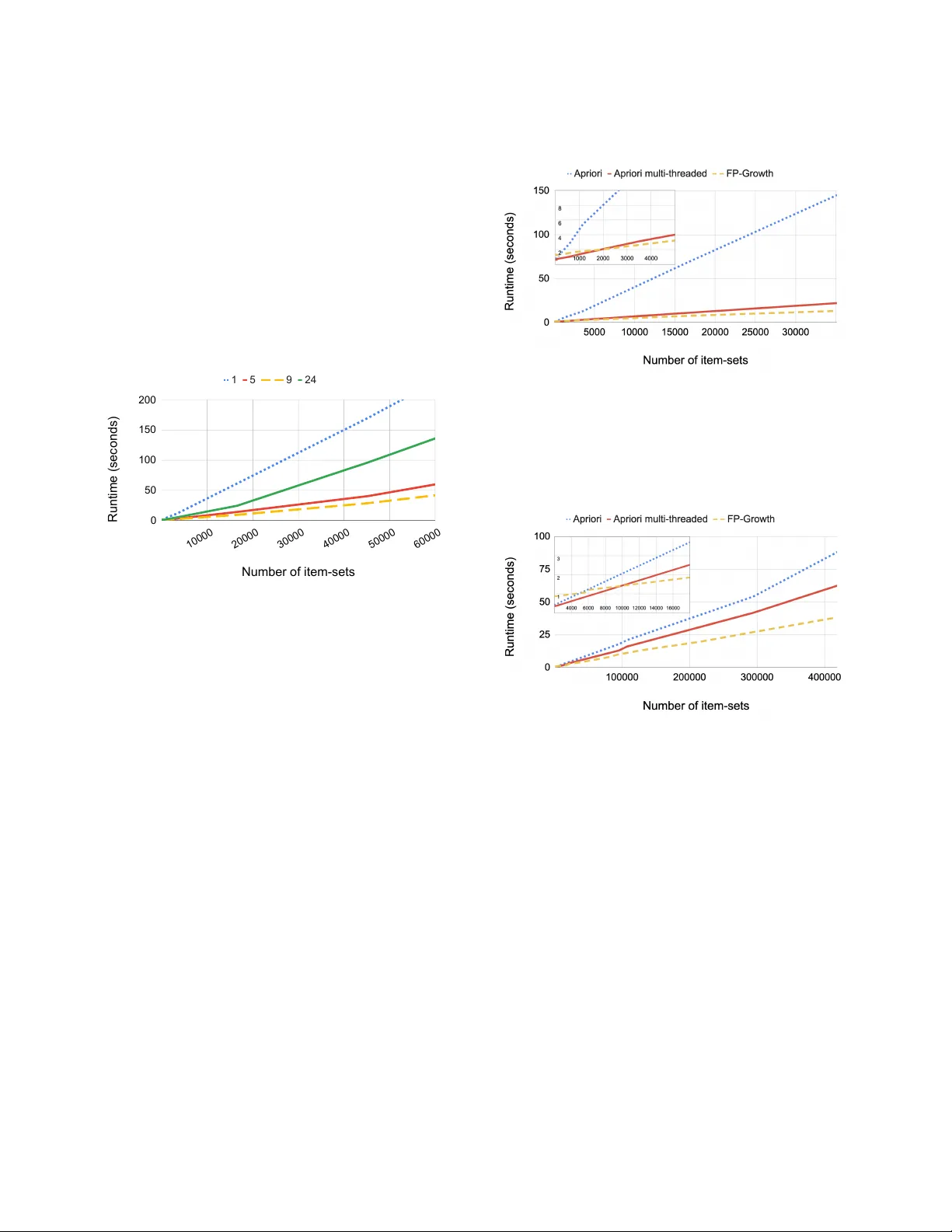
Original Paper
Loading high-quality paper...
Comments & Academic Discussion
Loading comments...
Leave a Comment