On Adaptive Linear-Quadratic Regulators

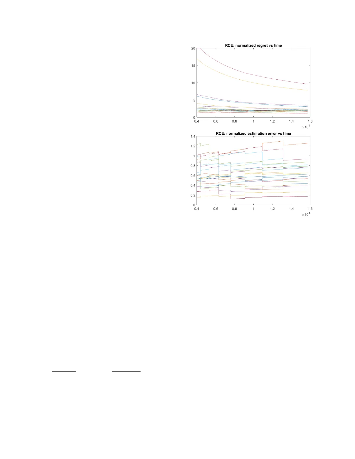
On Adaptiv e Linear-Quadratic Regulators Mohamad Kazem Shirani F aradon b eh, Am buj T ewari, and George Mic hailidis Abstract P erformance of adaptiv e con trol policies is assessed through the regret with respect to the optimal regulator, whic h reﬂects the increase in the operating cost due to uncertain ty about the dynamics parameters. Ho wev er, a v ailable results in the literature do not provide a quantitativ e characterization of the eﬀect of the unknown parameters on the regret. F urther, there are problems regarding the eﬃcien t implementation of some of the existing adaptive policies. Finally , results regarding the accuracy with whic h the system’s parameters are identiﬁed are scarce and rather incomplete. This study aims to comprehensively address these three issues. First, b y introducing a nov el decomp osition of adaptiv e p olicies, we establish a sharp expression for the regret of an arbitr ary p olicy in terms of the deviations from the optimal regulator. Second, we show that adaptive p olicies based on slight mo diﬁcations of the Certaint y Equiv alence scheme are eﬃcien t. Speciﬁcally , w e establish a regret of (nearly) square-root rate for tw o families of randomized adaptive policies. The presen ted regret bounds are obtained by using anti-c onc entr ation results on the random matrices emplo y ed for randomizing the estimates of the unknown parameters. Moreo ver, we study the minimal additional information on dynamics matrices that using them the regret will b ecome of logarithmic order. Finally , the rates at which the unknown parameters of the system are b eing identiﬁed are presented. Key wor ds: Regret Analysis; Certaint y Equiv alence; Randomized Algorithms; Thompson Sampling; System Identiﬁcation; Adaptiv e Policies. 1 In tro duction This w ork studies the problem of designing adaptive p olicies for the following Linear-Quadratic (LQ) system. Giv en an initial state x (0) ∈ R p , the system evolv es as x ( t + 1) = A 0 x ( t ) + B 0 u ( t ) + w ( t + 1) , (1) for t ≥ 0, where the vector x ( t ) ∈ R p corresp onds to the state (and also output) of the system at time t , u ( t ) ∈ R r is the control input, and { w ( t ) } ∞ t =1 denotes a sequence of random disturbances. F urther, the instan ta- neous quadratic cost of the con trol la w b π is denoted by c t ( b π ) = x ( t ) 0 Qx ( t ) + u ( t ) 0 Ru ( t ) , (2) where Q ∈ R p × p , R ∈ R r × r are symmetric positive deﬁ- nite matrices, and x ( t ) 0 , u ( t ) 0 denote the transp ose of the v ectors x ( t ) , u ( t ). The dynamics of the system, i.e., b oth the transition matrix A 0 ∈ R p × p , as w ell as the input matrix B 0 ∈ R p × r , are ﬁxed and unknown , while Q, R are assumed known. The ov erall ob jective is to adap- tiv ely regulate the system in order to minimize its long- term av erage cost. Although regulation of LQ systems represents a canon- ical problem in optimal con trol, adaptiv e p olicies ha ve not b een adequately studied in the literature. In fact, a large num b er of classical pap ers fo cuses on the setting of adaptiv e tracking, where the ob jective is to steer the sys- tem to track a reference tra jectory [1,2,3,4,5,6,7,8,9]. So, b ecause the op erating cost is not directly a function of the con trol signal (i.e., R = 0), analysis of adaptive reg- ulators b ecomes diﬀerent and less technically in volv ed. Therefore, existing results are not applicable to general LQ systems, wherein both the state and the control in- put impact the op erating cost. The adaptiv e Linear- Quadratic Regulators (LQR) problem has been studied in the literature [10,11,12,13,14,15,16,17], but there are still gaps that the present w ork aims to ﬁll by addressing cost optimalit y , parameter estimation, and the trade-oﬀ b et w een identiﬁcation and control. Since the system’s dynamics are unknown, learning the k ey parameters A 0 , B 0 is needed for designing an op- timal regulation p olicy . Ho wev er, the system op erator needs to apply some control inputs, in order to collect data (observ ations) for parameter estimation. A p opu- lar approach to design an adaptive regulator is Certaint y Equiv alence (CE) [18]. In tuitively , its prescription is to apply a control policy as if the estimated parameters are the true ones guiding the system’s evolu tion. In gen- eral, the ineﬃciency (as well as the inconsistency) of CE [12,19,20] has led researc hers to consider sev eral mo diﬁ- cations of the CE approach. One idea is to use the principle of Optimism in the F ace of Uncertaint y (OFU) [13,14,15] (also known as b et on the b est [12], and the cost-biased approach [10]). OFU recommends to apply the optimal regulators b y treat- ing optimistic appro ximations of the unkno wn matrices as the true dynamics [21]. Another idea is to replace the p oin t estimate of the system parameters by a p osterior distribution whic h is obtained through Bay es law b y in- tegrating a prior distribution and the likelihoo d of the data collected so far. One then dra ws a sample from this p osterior distribution and applies the optimal p olicy , as if the system ev olv es according to the sampled dynam- ics matrices. This approac h is known as Thompson (or p osterior) sampling [16,17]. Note that most of the existing w ork in the literature is purely asymptotic in nature so that it establishes the con v ergence of the adaptive aver age cost to the opti- mal v alue. It includes adaptiv e LQRs based on the OFU principle [10,12], as well as those based on the metho d of random p erturbations b eing applied to contin uous time Ito pro cesses [11]. How ever, results on the sp eed of con- v ergences are rare and rather incomplete. On the other hand, from the identiﬁcation viewp oint, consistency of parameter estimates is lac king for general dynamics ma- trices [22,23]. Moreov er, accuracy rates for estimation of system parameters are only provided for minimum- v ariance problems [8,9]. Indeed, the estimation rate for matrices describing the system’s dynamics is not cur- ren tly av ailable for general LQ systems. Since in many applications the eﬀective horizon is ﬁ- nite, the aforemen tioned asymptotic analyses are practi- cally less relev ant. Th us, addressing the optimalit y of an adaptiv e strategy under more sensitiv e criteria is needed. F or this purpose, one needs to comprehensiv ely examine the r e gr et ; i.e., the cum ulative deviation from the opti- mal p olicy . Regret analyses are th us far limited to re- cen t work addressing OFU adaptive p olicies [13,14,15], and results for TS obtained under restricted conditions [16,17]. One issue with OFU is the computational in- tractabilit y of ﬁnding an optimistic approximation of the true parameters, since it needs to solve lots of non-conv ex matrix optimization problems. More imp ortantly , w e sho w that the existing regret b ounds [13,14,15,16,17] can b e achiev ed or improv ed through simpler adaptiv e reg- ulators. A key contribution of this work is a remark ably gen- eral result to address the p erformance of control p olicies. Namely , tailoring a nov el metho d for regret decomp osi- tion, we utilize some results from martingale theory to establish Theorem 1. It pro vides a sharp expression for the regret of arbitrary regulators in terms of the devia- tions from the optimal feedback. Lev eraging Theorem 1, w e analyze t wo families of CE-based adaptive p olicies. First, we show that the gro wth rate of the regret is (nearly) square-root in time (of the in teraction with the system), if the CE regulator is properly r andomize d . Per- formance analyses are presented for b oth common ap- proac hes of additive randomization and p osterior sam- pling. Then, the adaptiv e LQR problem is discussed when additional information (regarding the unkno wn dynamics parameters of the system) is av ailable. In this case, a lo garithmic rate for the regret of generalizations of CE adaptive p olicies is established, assuming that the a v ailable side information satisﬁes an iden tiﬁability con- dition. Examples of side information include constraints on the rank or the supp ort of dynamics matrices, that in turn lead to optimality of the linear feedback regulator, if the closed-loop matrix is accurately estimated. F ur- ther, the identiﬁcation p erformance of the corresp ond- ing adaptive regulators is also addressed. T o the b est of our knowledge, this work pro vides the ﬁrst compre- hensiv e study of CE-based adaptive LQRs, for b oth the iden tiﬁcation and the regulation problem. The remainder of the pap er is organized as follows. The problem is formulated in Section 2. Then, we provide an expression for the regret of general adaptive policies in Subsection 3.1. Subsequen tly , the consistency of estimat- ing the dynamics parameter is giv en in Subsection 3.2. In Section 4, we study the gro wth rate of the regret, as w ell as the accuracy of parameter estimation, for tw o randomization sc hemes. Finally , in Section 5 we study a general condition which leads to signiﬁcan t p erformance impro v ements in both regulation and identiﬁcation. Remark 1 (Sto c hastic statements) Al l pr ob abilis- tic e qualities and ine qualities thr oughout this p ap er hold almost sur ely, unless otherwise explicitly mentione d. The following notation will be used throughout this pap er. F or a matrix A ∈ C k × ` , A 0 denotes its trans- p ose. When k = ` , the smallest (resp ectively largest) eigen v alue of A (in magnitude) is denoted b y λ min ( A ) (resp ectiv ely λ max ( A )). F or v ∈ C d , deﬁne the norm | | v | | =  d P i =1 | v i | 2  1 / 2 . W e also use the follo wing nota- tion for the op erator norm of matrices. F or A ∈ C k × ` let | | | A | | | = sup | | v | | =1 | | Av | | . In order to show the dimension of the manifold M we employ dim ( M ). Finally , to indicate the order of magnitude, we use a n = O ( b n ) whenev er lim sup n →∞ | a n /b n | < ∞ , employ a n = Ω ( b n ) for lim inf n →∞ | a n /b n | > 0, and write a n  b n , as long as b oth a n = O ( b n ) , a n = Ω ( b n ) hold. 2 Problem F ormulation W e start by deﬁning the adaptive LQR problem this w ork is addressing. The sto chastic evolution of the sys- tem is go verned b y the dynamics (1), where for all t ≥ 1, 2 w ( t ) is the vector of random disturbances satisfying: E [ w ( t )] = 0 , E [ w ( t ) w ( t ) 0 ] = C , and | λ min ( C ) | > 0. F or the sak e of simplicit y , the noise vectors { w ( t ) } ∞ t =1 are assumed to b e indep endent ov er time t . The latter as- sumption is made to simplify the presentation, and gen- eralization to martingale diﬀerence sequences (adapted to a ﬁltration) is straightforw ard 1 . F urther, the follow- ing moment condition for the noise process is assumed. Assumption 1 (Moment condition) Ther e is α > 4 , such that α -th moments exist: sup t ≥ 1 E [ | | w ( t ) | | α ] < ∞ . In addition, we assume that the true dynamics of the un- derlying system are stabilizable, a minimal assumption for the optimal control problem to be well-posed. Assumption 2 (Stabilizability) The true dynamics [ A 0 , B 0 ] is stabilizable: ther e exists a stabilizing fe e db ack L ∈ R r × p such that | λ max ( A 0 + B 0 L ) | < 1 . Note that Assumption 2 implies stabilizability in the a v erage sense: lim sup n →∞ n − 1 n P t =0 | | x ( t ) | | 2 < ∞ . Deﬁnition 1 Henc eforth, for A ∈ R p × p , B ∈ R p × r , we use θ to denote [ A, B ] . So, θ ∈ R p × q , wher e q = p + r . W e assume p erfe ct observ ations; i.e., the output of the system corresp onds to the state vector x ( t ). Next, an admissible con trol p olicy is a mapping π that designs the input according to the dynamics matrices A 0 , B 0 , the cost matrices Q, R , and the history of the system: u ( t ) = π  A 0 , B 0 , Q, R, { x ( i ) } t i =0 , { u ( j ) } t − 1 j =0  , for all t ≥ 0. An adaptive p olicy such as b π , is oblivious to the dynamics parameter θ 0 ; i.e., u ( t ) = b π  Q, R, { x ( i ) } t i =0 , { u ( j ) } t − 1 j =0  . When applying the p olicy π , the resulting instantaneous quadratic cost at time t deﬁned in (2) is denoted b y c t ( π ). F or an arbitrary p olicy π , let J π ( A 0 , B 0 ) denote the exp ected a verage cost of the system: J π ( A 0 , B 0 ) = lim sup n →∞ n − 1 n − 1 P t =0 E [ c t ( π )]. Note that the dep endence of J π ( θ 0 ) to the known cost matrices Q, R is suppressed. Then, the optimal exp ected av erage cost is deﬁned as J ? ( A 0 , B 0 ) = min π J π ( A 0 , B 0 ), where the minim um is tak en ov er al l admissible con trol policies. T he following 1 It suﬃces to replace the in volv ed terms with those consist- ing of the conditional expressions (w.r.t. the corresp onding ﬁltration). prop osition provides an optimal p olicy for minimizing the av erage cost, based on the Riccati equations: K ( θ ) = Q + A 0 K ( θ ) A − A 0 K ( θ ) B ( B 0 K ( θ ) B + R ) − 1 B 0 K ( θ ) A, (3) L ( θ ) = − ( B 0 K ( θ ) B + R ) − 1 B 0 K ( θ ) A. (4) Accordingly , deﬁne the linear time-inv ariant p olicy π ? : π ? : u ( t ) = L ( θ 0 ) x ( t ) , t = 0 , 1 , 2 , · · · . (5) Prop osition 1 (Optimal p olicy [24,25,26]) If [ A 0 , B 0 ] is stabilizable, (3) has a unique solution, and π ? deﬁne d in (5) is an optimal r e gulator. Conversely, if K ( θ 0 ) is a solution of (3) , L ( θ 0 ) deﬁne d by (4) is a stabilizer. In the latter case of Prop osition 1, the solution K ( θ 0 ) is unique and π ? is an optimal regulator. Note that although π ? is the only optimal p olicy among the time- in v arian t feedbac k regulators, there are uncountably man y time v arying optimal controllers. T o rigorously set the stage, we denote the linear reg- ulator u ( t ) = L t x ( t ) by π = { L t } ∞ t =0 , where L t is a r × p matrix determined according to A 0 , B 0 , Q, R , { x ( i ) } t i =0 , { u ( j ) } t − 1 j =0 . F or time-in v ariant policy π 0 = { L 0 } ∞ t =0 , we use π 0 and L 0 in terc hangeably . F or an adaptiv e op erator, the dynamics matrices A 0 , B 0 are unkno wn. Hence, adaptiv e p olicy b π = n b L t o ∞ t =0 con- stitutes the linear feedbacks u ( t ) = b L t x ( t ), where b L t ∈ R r × p is required to b e determined according to Q, R , { x ( i ) } t i =0 , { u ( j ) } t − 1 j =0 . In order to measure the eﬃ- ciency of an arbitrary regulator π , the resulting instan- taneous cost will b e compared to that of the optimal p olicy π ? deﬁned in (5). Sp eciﬁcally , the r e gr et of policy π at time n is deﬁned as R n ( π ) = n − 1 X t =0 [ c t ( π ) − c t ( π ? )] . (6) The comparison b etw een adaptive control p olicies is made according to regret, which is the cumulativ e de- viation of the instan taneous cost of the corresp onding adaptiv e p olicy from that of the optimal con troller π ? . An analogous expression for regret is previously used for the problem of adaptive tracking [1,2]. An alternativ e deﬁnition of the regret that has b een used in the existing literature [13,14,15,16,17] is the cum ulative deviations from the optimal aver age cost: n − 1 P t =0 [ c t ( π ) − J ? ( θ 0 )]. The expression ab ov e diﬀers from R n ( π ) by the term 3 n − 1 P t =0 c t ( π ? ) − n J ? ( θ 0 ), which is studied in the following result. Prop osition 2 We have lim sup n →∞ n − 1 P t =0 c t ( π ? ) − n J ? ( θ 0 ) n 1 / 2 log n < ∞ . Therefore, the aforemen tioned deﬁnitions for the regret are indiﬀer ent , as long as one can establish an upp er b ound of O  n 1 / 2  magnitude (mo dulo a logarithmic fac- tor) for either deﬁnition. Ho w ev er, deﬁning the regret b y (6) leads to more accurate analyses and tighter results (e.g. the regret sp eciﬁcation of Theorem 1, and the log- arithmic rate of Theorem 5). T o pro ceed, we in tro duce the following deﬁnition. Deﬁnition 2 F or a stabilizable p ar ameter θ ∈ R p × q , deﬁne e L ( θ ) =  I p , L ( θ ) 0  0 ∈ R q × p . W e can then express the closed-lo op matrices based on θ , e L ( θ ). F or arbitrary stabilizable θ 1 , θ 2 , if one applies the optimal feedback matrix L ( θ 1 ) to a system with dynamics parameter θ 2 , the resulting closed-lo op matrix is A 2 + B 2 L ( θ 1 ) = θ 2 e L ( θ 1 ). 3 General Adaptive Policies Next, we study the properties of general adaptiv e regula- tors. First, w e study the regulation viewpoint in Subsec- tion 3.1, and examine the regret of arbitrary linear poli- cies. Then, from an identiﬁcation viewp oint, consistency of parameter estimation is considered in Subsection 3.2. 3.1 R e gulation The main result of this subsection provides an expression for the regret of an arbitrary (i.e., either adaptive or non- adaptiv e) p olicy . According to the follo wing theorem, the regret of the regulator { L t } ∞ t =0 is of the same order as the summation of the squares of the deviations of the linear feedbacks L t from L ( θ 0 ). Note that it is stronger than the previously known result that expressed the re- gret as the summation of the deviations from L ( θ 0 ) (not squared) [13,14,15,16,17]. As will b e shown shortly , this diﬀerence changes the nature of b oth the low er-b ound, as well as the upper-b ound of the regret. Theorem 1 (Regret sp eciﬁcation) Supp ose that π = { L t } ∞ t =0 is a line ar p olicy. L etting { x ? ( t ) } ∞ t =0 b e the tr aje ctory under the optimal p olicy π ? , we have 0 < lim inf n →∞ R n ( π ) χ n + % n ≤ lim sup n →∞ R n ( π ) χ n + % n < ∞ , wher e % n = x ? ( n ) 0 K ( θ 0 ) x ? ( n ) − x ( n ) 0 K ( θ 0 ) x ( n ) , and χ n = n − 1 P t =0 | | ( L ( θ 0 ) − L t ) x ( t ) | | 2 . The ab ov e sp eciﬁcation for the regret is remark ably gen- eral, since p olicy π do es not need to satisfy any con- dition. Even for destabilized systems, the exp onential gro wth of the state (and so the regret) is captured b y χ n . Conceptually , χ n captures the eﬀect of the p ast sub- optimalit y { L t } n − 1 t =0 on the regret, while the inﬂuence of the sub-optimal feedback { L t } ∞ t = n to b e applied hence- forth is reﬂected in % n . This is formally stated in the follo wing result, whic h also addresses the magnitude of | | x ? ( n ) | | . According to Assumption 1, Corollary 1 sho ws that lim sup n →∞ n − 1 / 2 % n = 0. Corollary 1 We have lim sup n →∞ n − β | | x ? ( n ) | | = 0 , for al l β > 1 /α . F urther, letting L t = L ( θ 0 ) for t ≥ n , and π = { L t } ∞ t =0 , we get 0 < R ∞ ( π ) /χ ∞ < ∞ . Theorem 1 can be used for the sharp speciﬁcation of the p erformance of adaptiv e regulators. The immediate con- sequence of Theorem 1 provides a tigh t upper bound for the regret of an adaptive p olicy , in terms of the linear feedbac ks. Indeed, since the presented result is bidirec- tional and not just an upp er bound, it will also provide a general information theoretic low er b ound for the re- gret of an adaptiv e regulator. F or stabilized dynamics, it is shown that the smallest estimation error when us- ing a sample of size t is at least of the order t − 1 / 2 [27]. Th us, at time t , the error in the iden tiﬁcation of the un- kno wn dynamics parameter θ 0 is at le ast of the same order. Therefore, for the minimax growth rate of the re- gret, Theorem 1 implies the lo wer b ound log n . In other words, for an arbitrary adaptive policy b π , it holds that lim inf n →∞ (log n ) − 1 R n ( b π ) > 0. In general, the information theoretic low er b ound ab ov e is not known to b e op er ational ly ac hiev able because of the common trade-oﬀ b etw een estimation and control. W e will dis- cuss the reasoning b ehind the presence of such a gap in Section 4, which leads to the op erational low er b ound lim inf n →∞ n − 1 / 2 R n ( b π ) > 0. Nevertheless, in Section 5 we discuss settings where av ailability of some side informa- tion leads to an achiev able regret of logarithmic order. Next, we provide some intuition behind Theorem 1 and Corollary 1. The expression is in nature similar to the concept of memorylessness, as discussed b elow. The dynamics of the system in (1) indicate that the inﬂu- ence of non-optimal control inputs lasts forever. That is, if L t 1 x ( t 1 ) 6 = L ( θ 0 ) x ( t 1 ), then for all t > t 1 , the state v ector x ( t ) deviates from the optimal tra jectory { x ? ( t ) } ∞ t =0 , and future control inputs { u ( t ) } ∞ t = t 1 +1 can not fully c omp ensate this deviation. Ho wev er, according 4 to Theorem 1, the regret is dominated by the magni- tude of the square of the deviations of the non-optimal feedbac ks from L ( θ 0 ). In other words, if switching to the optimal feedbac k L ( θ 0 ) o ccurs, then the regret re- mains of the same order of the eﬀect of the non-optimal con trol inputs previously applied, and so is memoryless. 3.2 Identiﬁc ation Another consideration for an adaptive p olicy is the esti- mation (learning) problem. Since in general the op erator has no know le dge regarding the dynamics parameter θ 0 , a natural question to address is that of identifying θ 0 , in addition to examining cost optimalit y . In this subsec- tion, w e address the asymptotic estimation consistency of general adaptive p olicies. That is, a rigorous formula- tion of the relationship b etw een the estimable informa- tion (through observing the state of the system), and the desir e d optimality manifold is pro vided. On one hand, for a linear feedback L , the b est one can do by observing the state vectors is “closed-lo op iden- tiﬁcation” [5,15]; i.e., estimating the closed-loop matrix A 0 + B 0 L accurately . On the other hand, an adaptive p olicy is at le ast desired to provide a sub-linear regret; lim sup n →∞ R n ( b π ) n = 0 . (7) The ab ov e t w o asp ects of an adaptiv e p olicy pro vide the prop erties of the asymptotic uncertain ty ab out the true dynamics parameter θ 0 . By the uniqueness of L ( θ 0 ) according to Prop osition 1, the linear feedbacks of the adaptive p olicy b π = n b L t o ∞ t =0 require to conv erge to L ( θ 0 ). F urther, b π uniquely iden tiﬁes the asymptotic closed-lo op matrix lim t →∞ A 0 + B 0 b L t . This matrix accord- ing to (7) is supposed to be θ 0 e L ( θ 0 ). Putting the ab o ve together, the asymptotic uncertaint y is reduced to the set of parameters θ ∞ that satisfy L ( θ ∞ ) = L ( θ 0 ) , θ ∞ e L ( θ 0 ) = θ 0 e L ( θ 0 ) . (8) T o rigorously analyze this uncertaint y , w e introduce some additional notation. First, for an arbitrary stabi- lizable θ 1 , in tro duce the shifted null-space of the linear transformation e L ( θ 1 ) : R p × q → R p × p b y N ( θ 1 ) as: N ( θ 1 ) = n θ ∈ R p × q : θ e L ( θ 1 ) = θ 1 e L ( θ 1 ) o . (9) So, N ( θ 1 ) is indeed the set of parameters θ , such that the closed-lo op transition matrix of tw o systems with dynamics parameters θ , θ 1 will b e the same, if apply- ing the optimal linear regulator in (4) calculated for θ 1 . Hence, if the op erator regulates the system by feedback L ( θ 1 ), one can not iden tify θ , θ 1 . In other w ords, N ( θ 1 ) is the le arning c ap ability of adaptive regulators. Then, w e deﬁne the desir e d planning of adaptive p olicies as fol- lo ws. F or an arbitrary stabilizable θ 1 , deﬁne S ( θ 1 ) as the lev el-set of the optimal con troller function (4), which maps θ ∈ R p × q to L ( θ ) ∈ R r × p : S ( θ 1 ) =  θ ∈ R p × q : L ( θ ) = L ( θ 1 )  . (10) Therefore, S ( θ 1 ) is in fact the set of parameters θ , such that the calculation of optimal linear regulator (4) pro- vides the same feedback matrix for b oth θ , θ 1 . Intuitiv ely , N ( θ 0 ) reﬂects the identiﬁcation asp ect of the adaptive regulators by sp ecifying the accuracy of the parameter estimation procedure. Similarly , S ( θ 0 ) reﬂects the con- trol aspect, and sp eciﬁes the regulation p erformance in terms of optimality of the cost minimization pro cedure. Hence, the asymptotic uncertaint y ab out the true pa- rameter θ 0 is according to (8) limited to the set P 0 = S ( θ 0 ) ∩ N ( θ 0 ) . (11) The system theoretic interpretation is as follo ws. Assum- ing (7), P 0 is the smallest subset of dynamics parameters θ that one can iden tify according to the state and the in- put sequences. Thus, the consistency of identifying the true dynamics parameter θ 0 is equiv alent to P 0 = { θ 0 } . The following result establishes the prop erties of P 0 , and will b e used later to discuss the op erational optimalit y of adaptiv e regulators. It generalizes some results in the literature [22,23]. Theorem 2 (Consistency) The set P 0 deﬁne d in (11) is a shifte d line ar subsp ac e of dimension dim ( P 0 ) = ( p − rank ( A 0 )) r . Therefore, consistency of estimating θ 0 is automatic al ly guaran teed for an adaptive p olicy with a sublinear re- gret, only if A 0 is a full-rank matrix. In other words, eﬀectiv e control (exploitation) suﬃces for consistent es- timation (exploration) only if rank ( A 0 ) = p . F or exam- ple, the sublinear regret b ounds of OFU [13,15] imply consistency , assuming A 0 is of the full rank. Intuitiv ely , a singular A 0 precludes unique identiﬁcation of b oth of A 0 , B 0 b y (8). Note that the con v erse is alwa ys true: consistency of parameter estimation implies the sublin- earit y of the regret. Clearly , full-rankness of A 0 holds for almost all θ 0 (with resp ect to Leb esgue measure). 4 Randomized Adaptive Policies The classical idea to design an adaptive policy is the follo wing pro cedure kno wn as CE. At ev ery time n , its prescription is to apply the optimal regulator provided b y (4), as if the estimated parameter b θ n coincides exactly with the truth θ 0 . According to (1), a natural estimation pro cedure is to linearly regress x ( t + 1) on the cov ariates x ( t ) , u ( t ), using all observ ations collected so far; 0 ≤ t ≤ 5 n − 1. F ormally , the CE policy is n L  b θ n o ∞ n =1 , where b θ n is a solution of the least-squares estimator using the data observed until time n . That is, b θ n = arg min θ ∈ R p × q n − 1 X t =0       x ( t + 1) − θ e L  b θ t  x ( t )       2 . The issue with CE is that it is capable of adapting to a non-optimal regulation. T ec hnically , CE p ossibly fails to falsify an incorrect estimation of the true parame- ter [12]. Supp ose that at time n , the h yp othetical esti- mate of the true parameter is b θ n 6 = θ 0 . When applying the linear feedbac k L  b θ n  , the true closed-lo op tran- sition matrix will b e θ 0 e L  b θ n  . Then, if this matrix is the same as the (falsely) assumed closed-loop transition matrix b θ n e L  b θ n  , the estimation pro cedure can fail to falsify b θ n . So, if L  b θ n  6 = L ( θ 0 ), the adaptive p olicy is not guaranteed to tend to ward a b etter control feedback, and a non-optimal regulator will b e p ersistently applied. F ortunately , if sligh tly mo diﬁed, CE can a v oid unfalsiﬁ- able approximations of the true parameters. More pre- cisely , w e sho w that the set of unfalsiﬁable parameters deﬁned b elow is of zero Leb esgue measure; U ( θ 0 ) = n θ ∈ R p × q : θ 0 e L ( θ ) = θ e L ( θ ) o . (12) Note that b y (9), θ 1 ∈ U ( θ 2 ) if and only if θ 2 ∈ N ( θ 1 ). Recalling the discussion in the previous section, N ( θ 1 ) captures the estimation ability of adaptive regulators. That is, the set U ( θ 0 ) contains the matrices θ for whic h the h yp othetically assumed closed-lo op matrix is indis- tinguishable from the true one. The next lemma sets the stage for the subsequen t results whic h show that CE can b e eﬃcient, if it is suitably randomized. Lemma 1 (Unfalsiﬁable set) The set U ( θ 0 ) deﬁne d in (12) has L eb esgue me asur e zer o. 4.1 R andomize d Certainty Equivalenc e According to Lemma 1, we can av oid the pathological set U ( θ 0 ). As subsequen tly explained, it suﬃces to random- ize the least-squares estimates of θ 0 , with a small (dimin- ishing) p erturbation. First, such p erturbations are cho- sen to b e contin uously distributed o ver the parameter space R p × q , in order to ev ade U ( θ 0 ). F urther, since the linear transformation e L  b θ n  is randomly perturb ed, we can estimate the unknown dynamics parameter θ 0 . Note that as discussed in the previous section, the sequence n e L  b θ n o ∞ n =0 relates the estimation of θ 0 to the accu- rate identiﬁcation of the closed-lo op matrix θ 0 e L  b θ n  . Finally , according to Theorem 1, the magnitude of the random perturbation needs to diminish suﬃciently fast. Indeed, while a larger magnitude p erturbation helps to the impro vemen t of estimation, an eﬃcient regulation requires it to be suﬃciently small. Addressing this trade- oﬀ is the common dilemma of adaptive control. A t the end of this section, we will examine this trade-oﬀ based on prop erties of estimation metho ds and the tight spec- iﬁcation of the regret in Theorem 1. In the sequel, we present the R andomize d Certainty Equivalenc e (RCE) adaptiv e regulator. R CE is an episo dic algorithm as follo ws. First, when iden tifying a linear dynamical system using n observ ations, the estimation accuracy scales at rate n − 1 / 2 . Therefore, one can defer updating of the parameter estimates un- til collecting suﬃciently more data. This leads to the episo dic adaptive p olicies, where the linear feedbacks are up dated only after episo des of exp onentially growing lengths [15]. In RCE, the randomization of the parame- ter estimate is episo dic as w ell. Th us, calculation of the linear feedbacks L  b θ n  b y (4) will o ccur sparsely (only O (log n ) times, instead of n times), which remark ably reduces the computational cost of the algorithm. Algorithm 1 : RCE Input: γ > 1, and σ 0 > 0 Let L  b θ 0  b e a stabilizer for m = 0 , 1 , 2 , · · · do while n < b γ m c do Apply u ( n ) = L  b θ n  x ( n ) b θ n +1 = b θ n end while Up date the estimate b θ n b y (13) end for T o formally deﬁne R CE, let { φ m } ∞ m =0 b e a sequence of i.i.d. p × q random matrices with indep endent N  0 , σ 2 0  en tries, for a ﬁxed σ 0 > 0. This sequence will b e used to randomize the estimates. RCE has an arbitrary param- eter γ > 1 for determining the lengths of the episo des, and starts by an arbitrary initial estimate b θ 0 suc h that L  b θ 0  stabilizes the system. T o ﬁnd such initial esti- mates, one can employ the existing adaptive algorithm to stabilize the system in a short p erio d [26]. Late r on, w e will brieﬂy discuss the aforementioned stabilization algorithm. Then, for each time n ≥ 0, we apply the lin- ear feedback L  b θ n  . If n satisﬁes n = b γ m c for some 6 m ≥ 0, we up date the estimate by b θ n = e θ n + arg min θ ∈ R p × q n − 1 X t =0       x ( t + 1) − θ e L  b θ t  x ( t )       2 , (13) where e θ n =  n − 1 / 4 log 1 / 4 n  φ m is the random p ertur- bation. Otherwise, for n 6 = b γ m c , the p olicy do es not up- date the estimates: b θ n = b θ n − 1 . Note that since the dis- tribution of e θ n o v er p × q matrices is absolutely contin u- ous with resp ect to Lebesgue measure, b θ n is stabilizable (as well as con trollable [28,29]). Therefore, by Proposi- tion 1, the adaptive feedback L  b θ n  is well deﬁned. Remark 2 ( Non-Gaussian Randomization) In gen- er al, it suﬃc es to dr aw { φ m } ∞ m =0 fr om an arbitr ary dis- tribution with b ounde d pr ob ability density functions on R p × q such that sup m ≥ 1 E h | | | φ m | | | 4+  i < ∞ , for some  > 0 . As mentioned b efore, the rate γ determines the lengths of the episo des during which the algorithm uses b θ n , b efore up dating the estimate. Smaller v alues of γ corresp ond to shorter episodes and thus more up dates and additional randomization; i.e., the smaller γ is, the b etter the esti- mation p erformance of RCE is. Although we will shortly see that such an improv ement will not pro vide a b etter asymptotic rate for the regret, it sp eeds up the con ver- gence and so is suitable if the actual time horizon is not v ery large. F urther, it increases the n umber of times the Riccati equation (4) needs to b e computed. Therefore, in practice the op erator can decide γ according to the time length of interacting with the system, and the desired computational complexity . It is imp ortant especially if the ev olution of the real-world plant under control re- quires the feedbac k policy to be updated fast (compared to the time the op erator needs to calculate the linear feedbac k). The following theorem addresses the b eha v- ior of R CE, and shows that adaptive p olicies based on OFU [13,14,15] do not pro vide a b etter rate for the re- gret, while they imp ose a large computational burden b y requiring solving a matrix optimization problem. Theorem 3 (RCE rates) Supp ose that b π is RCE, and b θ n is the p ar ameter estimate at time n . Then, we have lim sup n →∞ R n ( b π ) n 1 / 2 log n < ∞ , lim sup n →∞          b θ n − θ 0          2 n − 1 / 2 log n < ∞ . Note that the analysis of RCE strongly leverages the sp eciﬁcation of the regret presen ted in Theorem 1. Fig. 1 illustrates the results of Theorem 3 b y depicting the p er- formance of RCE for γ = 1 . 2, and the dynamics and Figure 1. R CE performance: normalized regret  n − 1 / 2 log − 1 n  R n ( b π ) vs n (top), and normalized estima- tion error  n 1 / 4 log − 1 / 2 n           b θ n − θ 0          vs n (bottom). cost matrices in (14). Curv es of the normalized v alues of b oth the regret and the estimation error are depicted as a function of time, with the colors of the v arious curv es corresp onding to diﬀerent replicates of the sto chastic dy- namics, as w ell as the adaptive p olicy RCE. 4.2 Thompson Sampling Another approach in existing literature is Thompson Sampling (TS), which has the follo wing Bay esian inter- pretation. Applying an initial stabilizing linear feedbac k, TS up dates the estimate b θ n through p osterior sampling. That is, the operator dra ws a realization b θ n of the Gaus- sian p osterior for which the mean and the cov ariance matrix are determined by the data observ ed to date. F ormally , let Σ 0 ∈ R q × q b e a ﬁxed p ositive deﬁnite (PD) matrix, and choose a coarse approximation µ 0 ∈ R p × q of the truth θ 0 . W e will shortly explain an algorithmic pro cedure for computing such coarse approximations. F urther, similar to R CE, ﬁx the rate γ > 1. Then, at eac h time n ≥ 0, we apply L  b θ n  , where b θ n is designed as follows. If n satisﬁes n = b γ m c for some m ≥ 0, b θ n is 7 A 0 =     1 . 04 0 − 0 . 27 0 . 52 − 0 . 81 0 . 83 0 0 . 04 − 0 . 90     , B 0 =     − 0 . 47 0 . 61 − 0 . 29 − 0 . 50 0 . 58 0 . 25 0 . 29 0 − 0 . 72     , Q =     0 . 65 − 0 . 08 − 0 . 14 − 0 . 08 0 . 57 0 . 26 − 0 . 14 0 . 26 2 . 50     , R =     0 . 20 0 . 05 0 . 08 0 . 05 0 . 14 0 . 04 0 . 08 0 . 04 0 . 24     . (14) dra wn from a Gaussian distribution N  µ m , Σ − 1 m  , where µ m = arg min µ ∈ R p × q b γ m c− 1 X t =0       x ( t + 1) − µ e L  b θ t  x ( t )       2 , (15) Σ m = Σ 0 + b γ m c− 1 X t =0 e L  b θ t  x ( t ) x ( t ) 0 e L  b θ t  0 . (16) Algorithm 2 : TS Input: γ > 1 Let Σ 0 ∈ R q × q b e PD, and L  b θ 0  b e a stabilizer for m = 0 , 1 , 2 , · · · do while n < b γ m c do Apply u ( n ) = L  b θ n  x ( n ) b θ n +1 = b θ n end while Calculate µ m , Σ m b y (15), (16) Dra w all rows of b θ n from N  µ m , Σ − 1 m  end for Namely , for 1 ≤ i ≤ p , the i -th row of b θ n is drawn in- dep enden tly from a multiv ariate Gaussian distribution of mean µ ( i ) m (the i -th row of µ m ), and cov ariance ma- trix Σ − 1 m . Otherwise, for n 6 = b γ m c the p olicy do es not up date: b θ n = b θ n − 1 . Clearly , µ m is the least-squares es- timate and Σ m is the (unnormalized) empirical cov ari- ance of the data observ ed b y the end of episode m . Note that unlik e RCE, the randomization in TS is based on the state and control signals. The following result estab- lishes the performance rates for TS. Theorem 4 (TS rates) L et the adaptive p olicy b π b e TS, and the p ar ameter estimate b e b θ n . Then, we have lim sup n →∞ R n ( b π ) n 1 / 2 log 2 n < ∞ , lim sup n →∞          b θ n − θ 0          2 n − 1 / 2 log 2 n < ∞ . Note that the ab ov e upp er-b ounds diﬀer by those of Theorem 3 by a logarithmic factor. The p erformance of TS for γ = 1 . 2, and the matrices A 0 , B 0 , Q, R in (14) is depicted in Fig. 2. Clearly , the curves of the normal- ized regret and the normalized estimation error in Fig. 2 fully reﬂect the rates of Theorem 4. F or TS based adap- tiv e LQRs, the Bayesian r e gr et (i.e., the exp e cte d v alue Figure 2. TS performance: normalized regret  n − 1 / 2 log − 1 n  R n ( b π ) vs n (top), and normalized estima- tion error  n 1 / 4 log − 1 / 2 n           b θ n − θ 0          vs n (bottom). of the regret, wherein the expectation is tak en under the assumed prior) has b een shown to b e of a similar mag- nitude [17]. Of course, this heavily relies on a Gaussian prior imposed on the true θ 0 , and the (non-Bay esian) regret is known to b e of O  n 2 / 3  magnitude [16]. There- fore, Theorem 4 provides an impro ved regret bound for TS, thanks to Theorem 1. By assuming stronger assump- tions (e.g. b oundedness of the state), a similar result has b een recently established for the case p = 1, which holds uniformly ov er time [30]. F or the sake of completeness, we brieﬂy discuss an ex- isting adaptive stabilization pro cedure that one can emplo y b efore utilizing R CE or TS. First, in the work of F aradonbeh et al. [26], it is sho wn that for some ﬁxed  0 > 0, a coarse approximation b θ 0 that satisﬁes          b θ 0 − θ 0          ≤  0 , is suﬃcien t for stabilizing the sys- tem [26]. Note that the closed-lo op matrix can be un- 8 stable b efore termination of an stabilization pro cedure. On the other hand, there exists a pathological subset of unstable matrices such that if the closed-lo op tran- sition matrix b elongs to that subset, it is not feasible to b e accurately estimated [31]. Sp eciﬁcally , in order to ensure consistency , the true unstable closed-lo op tran- sition matrix during the stabilization p erio d needs to b e r e gular , as deﬁned below [31]. The unstable square matrix D is r e gular if the eigenspaces corresp onding to the eigenv alues of D outside the unit circle are one dimensional [31]. Then, it is established that random linear feedbac k matrices preclude the closed-lo op irreg- ularit y [26]. Therefore, the metho d of random feedback matrices guarantees that a coarse approximation of θ 0 is ac hiev able in ﬁnite time, and a stabilization set can b e constructed [26]. Thus, w e assume that the ini- tial linear feedback matrix L  b θ 0  is a stabilizer (i.e.,    λ max  θ 0 e L  b θ 0     < 1), and the system remains stable when R CE or TS is b eing emplo y ed. More details for establishing ﬁnite time adaptive stabilization are pro- vided in the aforementioned reference [26]. As a matter of fact, closed-loop regularity is not guaranteed, if only the control signals { u ( t ) } ∞ t =0 are randomized. F urther, the classical framework of p ersistent excitation is not applicable due to the possible instability of the closed- lo op matrix [31,32,33,34]. 4.3 Optimality Next, we discuss the reason for the presence of a signiﬁ- can t gap betw een the op erational regrets of Theorem 3 and Theorem 4, and the information theoretic low er b ound men tioned in Subsection 3.1. In fact, the follow- ing discussion shows that the logarithmic lo wer b ound is not practically ac hiev able. Nev ertheless, in the next sec- tion we show how using additional information for the true dynamics parameter yields a regret of logarithmic order. In the sequel, w e discuss an argument that leads to the following conjecture: the regret is op erationally of order n 1 / 2 . F or this purpose, we ﬁrst state the follow- ing lemma ab out the level-set manifold S ( θ 0 ) deﬁned in (10). It is a generalization of a previously established result for full-rank matrices [22,23]. Lemma 2 (Optimality manifold) The optimality level-set S ( θ 0 ) is a manifold of dimension dim ( S ( θ 0 )) = p 2 + ( p − rank ( A 0 )) ( r − rank ( B 0 )) at p oint θ 0 . By Theorem 2, we hav e dim ( S ( θ 0 )) − dim ( P 0 ) = k , where k = p 2 − ( p − rank ( A 0 )) rank ( B 0 ). The tan- gen t space of the manifold S ( θ 0 ) at p oin t θ 0 , shares ( p − rank ( A 0 )) r of its dimensions with N ( θ 0 ), and the other k dimensions are apart from N ( θ 0 ). Intuitiv ely , N ( θ 0 ) reﬂects the constrain t of estimating the dynam- ics parameter, and S ( θ 0 ) is the desired information to design an optimal p olicy . Thus, those k dimensions of S ( θ 0 ) which are not in N ( θ 0 ), c an not b e estimated unless the subspace N ( θ 0 ) is suﬃciently p erturb ed. Suc h a p erturbation is av ailable only through applying non-optimal feedbacks, which yields a larger regret than the logarithmic rate mentioned in Subsection 3.1. Next, w e carefully analyze the regret based on the lim- its in falsifying the parameters not b elonging to S ( θ 0 ). First, ineﬃciency of an adaptiv e regulator compared to the optimal feedback L ( θ 0 ) is determined by the un- certain t y for the exact sp eciﬁcation of the optimalit y manifold S ( θ 0 ). As an extreme example, supp ose that S ( θ 0 ) is provided to an op erator who do es not kno w θ 0 . Then, denoting the adaptiv e p olicy ab ov e by b π , we ha v e R n ( b π ) = 0. Theorem 1 states that if at time n the adaptiv e regulator approximates S ( θ 0 ) with error  n , the growth in the regret is in magnitude  2 n . Thus, it suﬃces to examine the estimation accuracy  n that in turn dep ends both on the iden tiﬁcation accuracy of the closed-lo op transition matrix, as w ell as the falsiﬁcation of dynamics parameters θ / ∈ S ( θ 0 ). No w, supp ose that the ob jective is to falsify θ 1 ∈ N ( θ 0 ), suc h that | | | θ 1 − θ 0 | | | = σ n , and θ 1 − θ 0 is orthogonal to the linear manifold P 0 deﬁned in (11). The latter prop- ert y of θ 1 dictates lim inf n →∞ σ − 1 n | | | L ( θ 1 ) − L ( θ 0 ) | | | > 0. The k ey point is that in order to falsify θ 1 , non-optimal lin- ear feedbacks need to b e applied suﬃciently many times. F or instance, if applying L ( θ 0 ), the estimation provides N ( θ 0 ), i.e., θ 1 can nev er get falsiﬁed. More generally , assume that L is a δ n -p erturbation of the optimal feed- bac k: | | | L − L ( θ 0 ) | | | = δ n . The shifted subspace of un- certain t y when applying L deviates from N ( θ 0 ) b y at most O ( δ n ) (in the sense of inner pro ducts of the unit v ectors). Next, assume that the operator applies L (or a similar δ n -p erturb ed feedback) for a duration of n time p oin ts. Note that the closed-lo op estimation error is at least of the order of n − 1 / 2 [27]. Thus, the op erator can falsify θ 1 only if lim inf n →∞ n 1 / 2 δ n σ n > 0. In other words, the adaptiv e regulator can av oid applying con trol feed- bac ks of distance at least n − 1 / 2 δ − 1 n from the optimal feedbac k, only if con trol feedbac ks of distance δ n are in adv ance applied for a perio d of length n . Hence, we ob- tain lim inf n →∞ σ − 2 n ( R n +1 ( b π ) − R n ( b π )) > 0 by using Theo- rem 1, which also implies that suc h p erturb ed feedbac ks imp ose a regret of the order nδ 2 n . Putting together, we get lim inf n →∞ R n ( b π ) ( R n +1 ( b π ) − R n ( b π )) > 0. It leads to the follo wing conjecture which constitutes an interesting direction for future work. Conjecture 1 (low er b ound) F or an arbitr ary adaptive p olicy b π we have lim inf n →∞ n − 1 / 2 R n ( b π ) > 0 . Note that if the ab ov e conjecture is true, R CE and TS pro vide a nearly optimal b ound for the regret. Ev en the logarithmic gap b etw een the low er and upp er b ounds is inevitable, due to the existence of an analogous gap in 9 the closed-loop iden tiﬁcation of linear systems [27]. F ur- ther, the ab ov e discussion explains the intuition behind the design of R CE. Sp eciﬁcally , the magnitude of the p erturbation          e θ n          according to the ab ov e discussion is optimally selected, since it satisﬁes 0 < lim inf n →∞ σ − 1 n δ n ≤ lim sup n →∞ σ − 1 n δ n < ∞ , mo dulo a logarithmic factor. In- deed, if randomization is (signiﬁcan tly) smaller in mag- nitude than n − 1 / 4 , the portion of the regret due to such a p erturbation will reduce. How ever, it also reduces the accuracy of the parameter estimate. Th us, the other por- tion of the regret due to estimation error will increase. A similar discussion holds for larger magnitudes of the p erturbation e θ n . On the other hand, the magnitude of randomization in TS is determined b y the collected ob- serv ations. As one can see in the pro of of Theorem 4, a similar magnitude of randomization is automatically imp osed by the structure of TS adaptiv e LQR. 5 Generalized Certaint y Equiv alence It is p ossible that the op erator has additional informa- tion on the dynamics. Examples of such information are the set of non-zero entries of θ 0 , the rank of θ 0 , or a plan t whose subsystems evolv e indep endently of each other. Another example comes from large netw ork sys- tems, where a substantial p ortion of the matrix θ 0 en- tries are zero [29]. F urther, it is easy to see that the tran- sition matrix of a system whose dynamics exhibit longer memory has a sp eciﬁc form [7,31]. In suc h cases, this additional structural information on θ 0 can b e used by the op erator in order to obtain a smaller regret for the adaptive regulation of the system. Nev ertheless, a comprehensive theory needs to formalize ho w this side information can provide theoretical sharp b ounds for the regret. In this section, we provide an iden- tiﬁabilit y condition that ensures that the adaptive LQRs attain the informational lo wer b ound of logarithmic or- der. In addition to the classical CE adaptive regulator, w e also consider the family of CE-based schemes which pro vide a logarithmic order of magnitude for the regret. First, we introduce the Gener alize d Certainty Equiv- alenc e (GCE) adaptive regulator. GCE is an episo dic algorithm with exponentially gro wing duration of episo des. Instead of randomizing the parameter esti- mate similar to RCE and TS, in GCE the least-squares estimate is perturb ed with an arbitrary matrix e θ n . Sup- p ose that the op erator knows that θ 0 ∈ Γ 0 , based on side information Γ 0 ⊂ R p × q . Then, ﬁxing the rate γ > 1, at time n ≥ 0, w e apply the controller L  b θ n  . If n satisﬁes n = b γ m c for some m ≥ 0, we up date the estimate by b θ n = e θ n + arg min θ ∈ Γ 0 n − 1 X t =0       x ( t + 1) − θ e L  b θ t  x ( t )       2 , (17) where e θ n is arbitr ary , and satisﬁes lim sup n →∞ n 1 / 2          e θ n          < ∞ . F or n 6 = b γ m c the p olicy does not up date: b θ n = b θ n − 1 . Note that if e θ n = 0, w e get the episo dic CE adaptive regulator. T o pro ceed, w e deﬁne the following condition. Algorithm 3 : GCE Inputs: γ > 1, Γ 0 ⊂ R p × q Let L  b θ 0  b e a stabilizer for m = 0 , 1 , 2 , · · · do while n < b γ m c do Apply u ( n ) = L  b θ n  x ( n ) b θ n +1 = b θ n end while Up date the estimate b θ n b y (17) end for Deﬁnition 3 (Identiﬁabilit y) Supp ose that ther e is Γ 0 ⊂ R p × q such that θ 0 ∈ Γ 0 . Then, θ 0 is identiﬁable, if for some β 0 < ∞ and al l stabilizable θ 1 , θ 2 ∈ Γ 0 : | | | L ( θ 2 ) − L ( θ 0 ) | | | ≤ β 0          ( θ 2 − θ 0 ) e L ( θ 1 )          . (18) In tuitiv ely , the deﬁnition abov e describes settings where side information Γ 0 is suﬃcient in the sense that an  -accurate identiﬁcation of the closed-lo op matrix (the RHS of (18)) provides an O (  )-accurate approximation of the optimal linear feedbac k (the LHS of (18)). Sub- sequen tly , we provide concrete examples of Γ 0 , such as presence of sparsity or low-rankness in θ 0 . Essentially , a ﬁnite union of manifolds of prop er dimension in the space R p × q suﬃces for identiﬁabilit y . T o see that, w e use the critical subsets N ( θ 0 ) , S ( θ 0 ), and P 0 deﬁned in (9), (10), and (11), resp ectively . First, note that P 0 ⊂ S ( θ 0 ) pro vides the opti- mal linear feedbac k L ( θ 0 ). Hence, for θ 1 ∈ N ( θ 0 ), | | | L ( θ 1 ) − L ( θ 0 ) | | | and inf θ ∈P 0 | | | θ 1 − θ | | | are of the same order of magnitude. Then, according to Theorem 2, b oth N ( θ 0 ) and P 0 are shifted linear subspaces pass- ing through θ 0 . Since dim ( N ( θ 0 )) = pr , the n ull-space N ( θ 0 ) shares ( p − rank ( A 0 )) r dimensions with P 0 , and has dim ( N ( θ 0 )) − dim ( P 0 ) = rank ( A 0 ) r dimensions orthogonal to P 0 . The regret of an adaptive regulator b π b ecomes larger than a logarithmic function of time, b ecause of the uncertaint y N ( θ 0 ) / P 0 . In other w ords, although the RHS of (18) is estimated accurately , the 10 aforemen tioned uncertaint y precludes obtaining an accurate approximation for the LHS of (18). In Deﬁ- nition 3, additional kno wledge ab out θ 0 remo v es suc h uncertain t y . Th us, a manifold (or a ﬁnite union of man- ifolds) of dimension pq − rank ( A 0 ) r implies the afore- men tioned iden tiﬁability condition. Below, we provide some examples of Γ 0 . (i) Optimality manifold: obviously , a trivial example is Γ 0 = S ( θ 0 ). In this case, the LHS of (18) v anishes. (ii) Support condition: let Γ 0 b e the set of p × q ma- trices with a priori known supp ort I . That is, for some set of indices I ⊂ { ( i, j ) : 1 ≤ i ≤ p, 1 ≤ j ≤ q } , en tries of all matrices θ ∈ Γ 0 are zero outside of I ; Γ 0 = { θ = [ θ ij ] : θ ij = 0 for ( i, j ) / ∈ I } . Then, Γ 0 is a (basic) subspace of R p × q and can satisfy the identiﬁa- bilit y condition (18). Note that it is necessary to hav e dim (Γ 0 ) = |I | ≤ pq − rank ( A 0 ) r . (iii) Sparsity condition: let Γ 0 b e the set of all p × q matrices with at most pq − rank ( A 0 ) r non-zero entries. Then, Γ 0 is the union of the matrices with support I for diﬀeren t sets I . Hence, the previous case implies that Γ 0 is a ﬁnite union of manifolds of prop er dimension. (iv) Rank condition: let Γ 0 b e the set of p × q matrices θ such that rank ( θ ) ≤ d . Then, Γ 0 is a ﬁnite union of manifolds of dimension at most d ( p + q − d ) [35]. Hence, if d ( p + q − d ) ≤ pq − rank ( A 0 ) r , and (18) holds, θ 0 is identiﬁable. (v) Subspace condition: for k = rank ( A 0 ) r , let { θ i } k i =1 b e p × q matrices such that θ i e L ( θ 0 ) = 0. Supp ose that θ 1 , · · · , θ k are linearly indep endent: if k P i =1 a i θ i = 0, then a 1 = · · · = a k = 0. Deﬁne Γ 0 = { θ + θ 0 : tr ( θ 0 θ i ) = 0 for all 1 ≤ i ≤ k } . If for all 1 ≤ i ≤ k it holds that θ 0 + θ i / ∈ P 0 , then Γ 0 satisﬁes the identiﬁabilit y condition of Deﬁnition 3. The follo wing Theorem establishes the optimality of GCE under the identiﬁabilit y assumption. As men- tioned in Section 4, a logarithmic gap b et w een the low er and upp er b ounds for the regret is inevitable due to similar limitations in system identiﬁcation [27]. Theorem 5 (GCE Rates) Supp ose that θ 0 is identi- ﬁable and the adaptive p olicy b π c orr esp onds to GCE. Deﬁning P 0 by (11) , let b θ n b e the p ar ameter estimate at time n . Then, we have lim sup n →∞ R n ( b π ) log 2 n < ∞ , lim sup n →∞ inf θ ∈P 0          b θ n − θ          2 n − 1 log n < ∞ . Comparing the ab ov e result with Theorem 3 and The- orem 4, the identiﬁabilit y assumption leads to signif- ican t improv ements in rates of b oth the regret and the estimation error. Moreov er, if rank ( A 0 ) = p , then P 0 = { θ 0 } . Th us, the estimation accuracy in Theorem 5 b ecomes: lim sup n →∞ n  log − 1 n           b θ n − θ 0          2 < ∞ . Finally , Theorem 5 improv es an existing result for iden tiﬁable systems. That is, under stronger assumptions, Ibrahimi et al. [14] sho w the regret b ound O  n 1 / 2 log 2 n  for adaptiv e p olicies based on OFU. How ever, according to Theorem 5, the regret of GCE is O  log 2 n  . 6 Concluding Remarks The performances of adaptiv e p olicies for LQ systems is addressed in this w ork, including b oth asp ects of regu- lation and identiﬁcation. First, w e established a general result whic h speciﬁes the regret of an arbitrary adaptive regulator in terms of the deviations from the optimal feedbac k. This tight bidirectional result provides a p o w- erful to ol to analyze the subsequen tly presen ted p olicies. That is, w e sho w that sligh t mo diﬁcations of CE pro vide a regret of (nearly) square-ro ot magnitude. The mo di- ﬁcations consist of tw o basic approaches of randomiza- tion: additive randomness, and Thompson sampling. In addition, w e formulated a condition which leads to lo g- arithmic regret. The rates of identiﬁc ation are also dis- cussed for the corresp onding adaptiv e regulators. Rigorous establishment of the prop osed op erational lower b ound for the regret is an interesting direction for future w orks. Besides, extending the developed frame- w ork to other settings such as switching systems, or those with imp erfe ct observ ations are topics of in terest. On the other hand, extensions to the dynamical mo d- els illustrating network systems (e.g., high-dimensional sparse dynamics matrices) is a challenging problem for further inv estigation. References [1] T. L. Lai and C.-Z. W ei, “Extended least squares and their applications to adaptive con trol and prediction in linear systems,” IEEE T r ansactions on Automatic Contr ol , v ol. 31, no. 10, pp. 898–906, 1986. [2] T. L. Lai, “Asymptotically eﬃcient adaptive control in stochastic regression models,” Advanc es in Applie d Mathematics , v ol. 7, no. 1, pp. 23–45, 1986. [3] L. Guo and H. Chen, “Con vergence rate of els based adaptive track er,” Syst. Sci & Math. Sci , vol. 1, pp. 131–138, 1988. [4] H.-F. Chen and J.-F. Zhang, “Conv ergence rates in stochastic adaptive tracking,” International Journal of Contr ol , vol. 49, no. 6, pp. 1915–1935, 1989. [5] P . Kumar, “Convergence of adaptive con trol schemes using least-squares parameter estimates,” IEEE T r ansactions on Automatic Contr ol , v ol. 35, no. 4, pp. 416–424, 1990. [6] T. L. Lai and Z. Ying, “Parallel recursive algorithms in asymptotically eﬃcien t adaptive c ontrol of linear stochastic systems,” SIAM journal on c ontr ol and optimization , vol. 29, no. 5, pp. 1091–1127, 1991. [7] L. Guo and H.-F. Chen, “The ˚ astrom-wittenmark self-tuning regulator revisited and els-based adaptive track ers,” IEEE T ransactions on Automatic Contr ol , vol. 36, no. 7, pp. 802– 812, 1991. 11 [8] B. Bercu, “W eigh ted estimation and tracking for armax models,” SIAM Journal on Contr ol and Optimization , vol. 33, no. 1, pp. 89–106, 1995. [9] L. Guo, “Conv ergence and logarithm laws of self-tuning regulators,” A utomatica , vol. 31, no. 3, pp. 435–450, 1995. [10] M. C. Campi and P . Kumar, “Adaptive linear quadratic gaussian control: the cost-biased approac h revisited,” SIAM Journal on Contr ol and Optimization , vol. 36, no. 6, pp. 1890–1907, 1998. [11] T. E. Duncan, L. Guo, and B. Pasik-Duncan, “Adaptive contin uous-time linear quadratic gaussian control,” IEEE T ransactions on automatic c ontr ol , vol. 44, no. 9, pp. 1653– 1662, 1999. [12] S. Bittan ti and M. C. Campi, “Adaptive control of linear time inv ariant systems: the b et on the b est principle,” Communic ations in Information & Systems , v ol. 6, no. 4, pp. 299–320, 2006. [13] Y. Abbasi-Y adkori and C. Szep esv´ ari, “Regret b ounds for the adaptive control of linear quadratic systems.” in COL T , 2011, pp. 1–26. [14] M. Ibrahimi, A. Jav anmard, and B. V. Roy , “Eﬃcient reinforcement learning for high dimensional linear quadratic systems,” in Advanc es in Neural Information Pr oc essing Systems , 2012, pp. 2636–2644. [15] M. K. S. F aradon b eh, A. T ew ari, and G. Michailidis, “Optimism-based adaptive regulation of linear-quadratic systems,” IEEE T ransactions on Automatic Contr ol, arXiv:1711.07230 , 2017. [16] M. Ab eille and A. Lazaric, “Thompson sampling for linear-quadratic control problems,” in AIST A TS 2017- 20th International Confer enc e on Artiﬁcial Intel ligenc e and Statistics , 2017. [17] Y. Ouy ang, M. Gagrani, and R. Jain, “Con trol of unkno wn linear systems with thompson sampling,” in Communic ation, Contr ol, and Computing (Al lerton), 2017 55th Annual Allerton Confer enc e on . IEEE, 2017, pp. 1198–1205. [18] Y. Bar-Shalom and E. Tse, “Dual eﬀect, certaint y equiv alence, and separation in sto chastic control,” IEEE T ransactions on Automatic Contr ol , vol. 19, no. 5, pp. 494– 500, 1974. [19] T. L. Lai and C. Z. W ei, “Least squares estimates in sto chastic regression mo dels with applications to identiﬁcation and control of dynamic systems,” The A nnals of Statistics , pp. 154–166, 1982. [20] A. Beck er, P . Kumar, and C.-Z. W ei, “Adaptive control with the stochastic approximation algorithm: Geometry and conv ergence,” IEEE T ransactions on Automatic Contr ol , vol. 30, no. 4, pp. 330–338, 1985. [21] T. L. Lai and H. Robbins, “Asymptotically eﬃcient adaptiv e allocation rules,” Advanc es in applie d mathematics , vol. 6, no. 1, pp. 4–22, 1985. [22] J. W. Polderman, “On the necessity of identifying the true parameter in adaptive LQ control,” Systems & c ontrol letters , v ol. 8, no. 2, pp. 87–91, 1986. [23] ——, “A note on the structure of tw o subsets of the parameter space in adaptive control problems,” Systems & c ontr ol letters , vol. 7, no. 1, pp. 25–34, 1986. [24] S. Chan, G. Goo dwin, and K. Sin, “Conv ergence properties of the riccati diﬀerence equation in optimal ﬁltering of nonstabilizable systems,” IEEE T r ansactions on A utomatic Contr ol , vol. 29, no. 2, pp. 110–118, 1984. [25] C. De Souza, M. Gevers, and G. Goodwin, “Riccati equations in optimal ﬁltering of nonstabilizable systems having singular state transition matrices,” IEEE T r ansactions on Automatic Contr ol , vol. 31, no. 9, pp. 831–838, 1986. [26] M. K. S. F aradon b eh, A. T ew ari, and G. Michailidis, “Finite time adaptiv e stabilization of linear systems,” IEEE T ransactions on Automatic Control , v ol. 64, no. 8, pp. 3498– 3505, 2019. [27] M. Simcho witz, H. Mania, S. T u, M. I. Jordan, and B. Rech t, “Learning without mixing: T o w ards a sharp analysis of linear system identiﬁcation,” arXiv preprint arXiv:1802.08334 , 2018. [28] D. P . Bertsek as, Dynamic pr o gr amming and optimal c ontr ol . Athena Scientiﬁc Belmon t, MA, 1995, v ol. 1, no. 2. [29] M. K. S. F aradon b eh, A. T ew ari, and G. Michailidis, “Optimality of fast matching algorithms for random netw orks with applications to structural controllability ,” IEEE T r ansactions on Contr ol of Network Systems , vol. 4, no. 4, pp. 770–780, 2017. [30] M. Ab eille and A. Lazaric, “Improv ed regret b ounds for thompson sampling in linear quadratic control problems,” in International Confer enc e on Machine L e arning , 2018, pp. 1– 9. [31] M. K. S. F aradonbeh, A. T ewari, and G. Michailidis, “Finite time iden tiﬁcation in unstable linear systems,” Automatic a , vol. 96, pp. 342–353, 2018. [32] R. Johnstone and B. Anderson, “Global adaptive p ole placement: detailed analysis of a ﬁrst-order system,” IEEE tr ansactions on automatic c ontrol , vol. 28, no. 8, pp. 852– 855, 1983. [33] B. D. Anderson, “Adaptive systems, lack of p ersistency of excitation and bursting phenomena,” Automatic a , vol. 21, no. 3, pp. 247–258, 1985. [34] H.-M. Zhang, “F urther comments on nonstationarity identiﬁcation problems for autoregressive mo dels,” in 29th IEEE Confer enc e on De cision and Control . IEEE, 1990, pp. 3204–3205. [35] U. Shalit, D. W einshall, and G. Chechik, “Online learning in the embedded manifold of low-rank matrices,” Journal of Machine L e arning R ese arch , vol. 13, no. F eb, pp. 429–458, 2012. [36] T. L. Lai and C. Z. W ei, “Asymptotic prop erties of multiv ariate weigh ted sums with applications to sto chastic regression in linear dynamic systems,” Multivariate Analysis VI , pp. 375–393, 1985. 12 A Pro ofs of Main Results The pro ofs of the main theorems are given next. Pro ofs of auxiliary lemmas are deferred to the app endix. A.1 Pro of of Theorem 1 and Corollary 1 Giv en n ≥ 1, and the linear p olicy π = { L t } n − 1 t =0 , deﬁne the sequence of p olicies π 0 , · · · , π n as follows. π 0 = { L ( θ 0 ) , · · · , L ( θ 0 ) } , π 1 = { L 0 , L ( θ 0 ) , · · · , L ( θ 0 ) } , . . . π n = { L 0 , L 1 , · · · , L n − 1 } . Indeed, the p olicy π i applies the same feedback as π at ev ery time t < i , and then for t ≥ i switches to the optimal p olicy π ? . Clearly , π 0 = π ? , and π n = π . Since R n ( π ) = n X k =1 n − 1 X t =0 [ c t ( π k ) − c t ( π k − 1 )] , (A.1) it suﬃces to ﬁnd c t ( π k ) − c t ( π k − 1 ), for 1 ≤ k ≤ n , and 0 ≤ t ≤ n − 1. Fixing k , let { x ( t ) } n − 1 t =0 , { y ( t ) } n − 1 t =0 b e the state tra jectories under π k , π k − 1 , resp ectively . So, letting D = A 0 + B 0 L ( θ 0 ) and D k − 1 = A 0 + B 0 L k − 1 , we ha v e x ( t ) = y ( t ) for 0 ≤ t ≤ k − 1, as well as c t ( π k ) = c t ( π k − 1 ) for 0 ≤ t ≤ k − 2, and x ( k ) = D k − 1 x ( k − 1) + w ( k ). F urther, if k ≤ t ≤ n − 1, then y ( t ) = D t − k +1 x ( k − 1) + t X j = k D t − j w ( j ) , x ( t ) = D t − k D k − 1 x ( k − 1) + t X j = k D t − j w ( j ) . Therefore, w e hav e x ( t ) = y ( t ) + D t − k ∆ k − 1 x ( k − 1), for k ≤ t < n , where ∆ k − 1 = D k − 1 − D = B 0 ( L k − 1 − L ( θ 0 )) . Th us, for w e obtain c k − 1 ( π k ) − c k − 1 ( π k − 1 ) = x ( k − 1) 0  L 0 k − 1 RL k − 1 − L ( θ 0 ) 0 RL ( θ 0 )  x ( k − 1) . Similarly , denote P 0 = Q + L ( θ 0 ) 0 RL ( θ 0 ), and replace for x ( t ) to see that if k ≤ t < n , then c t ( π k ) − c t ( π k − 1 ) =  2 y ( t ) + D t − k ∆ k − 1 x ( k − 1)  0 P 0 D t − k ∆ k − 1 x ( k − 1) . T o pro ceed, plug-in for y ( t ) to get c t ( π k ) − c t ( π k − 1 ) = x ( k − 1) 0 F k − 1 ( t ) x ( k − 1) + η k − 1 ( t ), where ∆ k − 1 = D k − 1 − D leads to η k − 1 ( t ) = 2 x ( k − 1) 0 ∆ 0 k − 1 D 0 t − k P 0 t X j = k D t − j w ( j ) , F k − 1 ( t ) = D 0 k − 1 D 0 t − k P 0 D t − k D k − 1 − D 0 t − k +1 P 0 D t − k +1 . Next, letting z k = n − 1 P t = k η k − 1 ( t ), and G k = L 0 k − 1 RL k − 1 − L ( θ 0 ) 0 RL ( θ 0 ) + n − 1 P t = k F k − 1 ( t ), clearly n − 1 X t =0 [ c t ( π k ) − c t ( π k − 1 )] = x ( k − 1) 0 G k x ( k − 1) + z k . (A.2) T o pro ceed, for 0 ≤ j ≤ n let K j = ∞ P ` = n − j D 0 ` P 0 D ` . So, n − 1 X t = k F k − 1 ( t ) = D 0 k − 1 ( K n − K k ) D k − 1 − D 0 ( K n − K k ) D implies G k = E k + H k , where E k = − D 0 k − 1 K k D k − 1 + D 0 K k D , H k = L 0 k − 1 RL k − 1 − L ( θ 0 ) 0 RL ( θ 0 ) − D 0 K n D + D 0 k − 1 K n D k − 1 . The Lyapuno v equation (see [26]) K ( θ 0 ) − D 0 K ( θ 0 ) D = P 0 , (A.3) leads to K n = K ( θ 0 ). Thus, letting X = L k − 1 − L ( θ 0 ), M = B 0 0 K ( θ 0 ) B 0 + R , since M L ( θ 0 ) = − B 0 0 K ( θ 0 ) A 0 , after doing some algebra we get H k = L ( θ 0 ) 0 RX + X 0 RL ( θ 0 ) + D 0 K ( θ 0 ) B 0 X + X 0 RX + X 0 B 0 0 K ( θ 0 ) D + X 0 B 0 0 K ( θ 0 ) B 0 X = X 0 M X Hence, adding up the terms in (A.2), (A.1) implies that R n ( π ) = Z n + S n + T n , (A.4) where Z n = n P k =1 z k , S n = n − 1 P k =0 x ( k ) 0 E k +1 x ( k ), and T n = n − 1 P k =0     M 1 / 2 ( L k − L ( θ 0 )) x ( k )     2 . In order to inv estigate S n , w e use the dynamics x ( k ) = D k − 1 x ( k − 1) + w ( k ), 13 as well as D 0 K k +1 D = K k , to get x ( k ) 0 D 0 K k +1 D x ( k ) = x ( k − 1) 0 D 0 k − 1 K k D k − 1 x ( k − 1) + w ( k ) 0 K k w ( k ) + 2 w ( k ) 0 K k D k − 1 x ( k − 1) , for 0 < k < n . Substituting in the expression for S n , and denoting w (0) = x (0), the telescopic diﬀerences v anish: S n + x ( n ) 0 K ( θ 0 ) x ( n ) = n − 1 X k =0 2 w ( k + 1) 0 K k +1 D k x ( k ) + n X k =0 w ( k ) 0 K k w ( k ) . (A.5) Plugging D k x ( k ) = k X j =0  D j +1 w ( k − j ) + D j ∆ k − j x ( k − j )  , as w ell as x ? ( n ) = n P j =0 D n − j w ( j ), in (A.5), w e hav e e S n = S n + x ( n ) 0 K n x ( n ) − x ? ( n ) 0 K n x ? ( n ) = n P k =1 w ( k ) 0 K k ξ k , where ξ k = 2 k P ` =1 D ` − 1 ∆ k − ` x ( k − ` ). Moreo v er, it is straigh tforw ard to show that Z n = n − 1 P j =1 ζ 0 j w ( j ), where ζ j = 2 j P ` =1 n − 1 P t = j D 0 t − j P 0 D t − ` ∆ ` − 1 x ( ` − 1). Hence, ζ j = ( K n − K j ) ξ j implies e S n + Z n = n P k =1 w ( k ) 0 K n ξ k . Next, we use the follo wing lemma. Lemma 3 [19] Supp ose that for al l t ≥ 0 , y ( t + 1) , v ( t ) ar e G t me asur able, G t ⊆ G t +1 , and E [ v ( t + 1) |G t ] = 0 . Deﬁne the martingale ψ n = n P t =1 y ( t ) 0 v ( t ) , and let ϕ n = n P t =1 | | y ( t ) | | 2 . If sup t ≥ 0 E h | | v ( t + 1) | | 2    G t i < ∞ , then lim sup n →∞ | ψ n | < ∞ on ϕ ∞ < ∞ , lim sup n →∞ ψ n ϕ 1 / 2 n log ϕ n = 0 on ϕ ∞ = ∞ . T aking G t = σ  { w ( i ) } t i =1 , { x ( i ) } t i =0  , and v ( t ) = w ( t ), y ( t ) = ξ t , we can use Lemma 3 since Assumption 1 holds. So, stabilit y of D (Prop osition 1), and | λ min ( M ) | > 0, lead to n P k =1 | | ξ k | | 2 = O ( T n ). Th us, by (A.4), we get the desired result since e S n + Z n = O  T 1 / 2 n log T n  . Next, the ﬁrst statemen t in Corollary 1 follo ws from The- orem 1 in the work of Lai and W ei [36]. T o pro ve the second result, ﬁrst observe that S ∞ = S n , T ∞ = T n , and Z ∞ = Z n . F urthermore, note that for t ≥ n we ha v e c t ( π ) = x ( t ) 0 P 0 x ( t ), c t ( π ? ) = x ? ( t ) 0 P 0 x ? ( t ), as well as x ( t ) = D t − n x ( n ) + t X j = n +1 D t − j w ( j ) , x ? ( t ) = D t − n x ? ( n ) + t X j = n +1 D t − j w ( j ) . So, letting δ n = 2 ∞ X t = n t X j = n +1 ( x ( n ) − x ? ( n )) 0 D 0 t − n P 0 D t − j w ( j ) , b y (A.3) the following holds: ∞ X t = n [ c t ( π ) − c t ( π ? )] = x ( n ) 0 K n x ( n ) − x ? ( n ) 0 K n x ? ( n ) + δ n . Finally , | | x ( n ) − x ? ( n ) | | 2 =             n − 1 X j =0 D n − 1 − j ∆ j x ( j )             2 = O ( T n ) , (A.6) together with Lemma 3 imply δ n = O  T 1 / 2 n log T n  . A.2 Pro of of Theorem 2 First, for an arbitrary θ ∈ P 0 , since θ ∈ N ( θ 0 ), we ha ve A + B L ( θ 0 ) = A 0 + B 0 L ( θ 0 ) = D 0 . (A.7) Next, for an arbitrary ﬁxed unit matrix (in the F rob e- nius norm) X ∈ R r × p , let L = L ( θ 0 ) + X b e a lin- ear feedback matrix which stabilizes the system of dy- namics parameters θ . Note that according to Prop osi- tion 1, θ ∈ S ( θ 0 ) leads to    λ max  θ e L ( θ 0 )     < 1. Thus, | λ max ( A + B L ) | < 1, as long as  is suﬃciently small. Then, applying L to the system θ , w e get J L ( θ ) = tr ( P (  ) C ), where P (  ) is the unique solution of the Ly apuno v equation P (  ) − ( A + B L ) 0 P (  ) ( A + B L ) = Q + L 0 RL. (A.8) Note that according to (A.3) and (A.7), it holds that P (0) = K ( θ 0 ). Letting ∆ ( X ) = lim  → 0  − 1 ( P (  ) − P (0)), 14 (A.8) leads to ∆ ( X ) − D 0 0 ∆ ( X ) D 0 = X 0 N + N 0 X, (A.9) where N = R L ( θ 0 ) + B 0 K ( θ 0 ) D 0 . Next, θ ∈ S ( θ 0 ) im- plies that L ( θ 0 ) is an optimal linear feedbac k for the sys- tem of dynamics parameter θ . So, the directional deriv a- tiv e of J L ( θ ) with resp ect to L is zero in all directions. In the direction of X , the deriv ative is tr (∆ ( X ) C ). Since all abov e statemen ts hold regardless of the p ositive deﬁ- nite matrix C , (A.9) and tr (∆ ( X ) C ) = 0 imply N = 0; D 0 0 K ( θ 0 ) B = − L ( θ 0 ) 0 R. (A.10) Therefore, (A.10) is a necessary condition for θ ∈ P 0 . Note that according to (A.3) and (A.7), the necessary condition (A.10) implies the necessit y of D 0 0 K ( θ 0 ) A = K ( θ 0 ) − Q . F urther, for every input matrix B whic h satisﬁes (A.10), the transition matrix A will be uniquely determined by (A.7) as A = D 0 − B L ( θ 0 ). Con v ersely , supp ose that B is an arbitrary matrix which satisﬁes (A.10). Letting A = D 0 − B L ( θ 0 ), w e sho w that [ A, B ] = θ ∈ P 0 . F or this purp ose, since the ab ov e deﬁnition of A automatically leads to θ ∈ N ( θ 0 ), it suf- ﬁces to show θ ∈ S ( θ 0 ). W riting Y = B − B 0 , we get A = A 0 − Y L ( θ 0 ). Moreo v er, deﬁne G = A 0 K ( θ 0 ) A , H = B 0 K ( θ 0 ) A , M = B 0 0 K ( θ 0 ) B 0 + R , and S = B 0 0 K ( θ 0 ) Y + Y 0 K ( θ 0 ) B 0 + Y 0 K ( θ 0 ) Y . Then, we cal- culate the matrix V = Q + G − H 0 ( M + S ) − 1 H = Q + A 0 K ( θ 0 ) A − A 0 K ( θ 0 ) B ( B 0 K ( θ 0 ) B + R ) − 1 B 0 K ( θ 0 ) A. W riting A, B , G, H in terms of A 0 , B 0 , M , S, Y , we ha ve V = Q + A 0 0 K ( θ 0 ) A 0 + L ( θ 0 ) 0 S L ( θ 0 ) −  B 0 0 K ( θ 0 ) A 0 − S L ( θ 0 )  0 ( M + S ) − 1  B 0 0 K ( θ 0 ) A 0 − S L ( θ 0 )  Then, using ( M + S ) − 1 = M − 1 − ( M + S ) − 1 S M − 1 , (3), and M L ( θ 0 ) = − B 0 0 K ( θ 0 ) A 0 , V can b e written as V = K ( θ 0 ) + L ( θ 0 ) 0 S W , where W = L ( θ 0 ) − ( M + S ) − 1 ( S L ( θ 0 ) + B 0 0 K ( θ 0 ) A 0 ) = L ( θ 0 ) − ( M + S ) − 1 ( S + M ) L ( θ 0 ) = 0; i.e., V = K ( θ 0 ) is a solution of the Riccati equation (3) for θ . According to Prop osition 1, the solution is unique; which is K ( θ ) = K ( θ 0 ). Moreov er, L ( θ ) = − ( M + S ) − 1 H = L ( θ 0 ) sho ws that θ ∈ S ( θ 0 ). So far, w e ha v e sho wn that θ ∈ P 0 , if and only if (A.7) and (A.10) hold. Next, (A.10) is essen tially stating that ev- ery column of B − B 0 (whic h is a vector in R p ), is orthogonal to the all columns of K ( θ 0 ) D 0 . This veri- ﬁes that (A.10) sp eciﬁes a shifted linear subspace. T o ﬁnd the dimension, since B has r columns, and (A.7) uniquely determines A in terms of B , w e get dim ( P 0 ) = ( p − rank ( K ( θ 0 ) D 0 )) r . Finally , by p ositive deﬁniteness of Q , (A.3) implies rank ( K ( θ 0 )) = p . F urther, since D 0 =  I p − B 0 M − 1 B 0 0 K ( θ 0 )  A 0 , it suﬃces to show rank  I p − B 0 M − 1 B 0 0 K ( θ 0 )  = p. (A.11) If (A.11) do es not hold, there exists v ∈ R p suc h that v 6 = 0 and v = B 0 M − 1 B 0 0 K ( θ 0 ) v . So, v = B 0 e v where e v = M − 1 B 0 0 K ( θ 0 ) v ∈ R r . Thus, B 0 0 K ( θ 0 ) B 0 e v = B 0 0 K ( θ 0 ) v = M e v = [ B 0 0 K ( θ 0 ) B 0 + R ] e v , or equiv alently , R e v = 0. P ositiv e deﬁniteness of R im- plies that e v = 0, which contradicts B 0 e v 6 = 0. This prov es (A.11), which completes the proof. A.3 Pro of of Theorem 3 The pro of is based on a sequence of in termediate results. First, for i ≥ 1, let V i b e the (unnormalized) state co- v ariance during the i -th episode: V i = b γ i c− 1 P t = b γ i − 1 c x ( t ) x ( t ) 0 . Lemma 4 F or the matrix V i deﬁne d ab ove, the fol low- ings hold: | λ max ( V m ) | = O ( γ m ) , lim inf m →∞ γ − m | λ min ( V m ) | ≥ ( γ − 1) | λ min ( C ) | . Then, in order to study the b ehavior of the least-squares estimate in (13), deﬁne U i = b γ i c− 1 X t =0 e L  b θ t  x ( t ) x ( t ) 0 e L  b θ t  0 . Note that since the parameter b θ t remains set (not chang- ing) during eac h episo de, U i can be written in terms of V 1 , · · · , V i as follows. First, for all b γ i − 1 c ≤ t ≤ b γ i c − 1, the parameter estimate b θ t do es not c hange. So, if t b e- longs to the i -th episo de, deﬁne the linear feedback ma- trix is L i = L  b θ t  . Letting e L i = e L  b θ t  , we ha ve U i = i P j =1 e L j V j e L 0 j . Then, the smallest eigen v alue of U i follo ws a diﬀeren t low er bound compared to that of V i : Lemma 5 Deﬁne U m as ab ove. Then, we have lim inf m →∞ γ − m/ 2 | λ min ( U m ) | > 0 , and | λ max ( U m ) | = O ( γ m ) . Next, the following result states that the estimation ac- curacy is determined by the eigenv alues of U i . Lemma 6 [19] F or n = b γ m c , deﬁne b θ n , e θ n ac c or ding 15 to (13) . Then, we have          b θ n − e θ n − θ 0          2 = O  log | λ max ( U m ) | | λ min ( U m ) |  . Therefore, Lemma 5 leads to          b θ n − e θ n − θ 0          = O  n − 1 / 4 log 1 / 2 n  . Using the moment condition in Re- mark 2, Marko v’s inequality gives P  | | | φ m | | | > m 1 / 4  = O  m − 1 − / 4  . Thus, an application of the Borel-Cantelli Lemma leads to | | | φ m | | | = O  m 1 / 4  ; i.e.,          e θ n          = O  n − 1 / 4 log 1 / 2 n  . So, we get the desired result ab out the identiﬁcation rate:          b θ n − θ 0          = O  n − 1 / 4 log 1 / 2 n  . T o pro ceed, w e present the following auxiliary result whic h shows that a similar rate holds for the deviations from the optimal linear feedback. Lemma 7 [15] Ther e exist 0 <  0 , β L < ∞ , such that for al l stabilizable θ satisfying | | | θ − θ 0 | | | <  0 , the fol- lowing holds: | | | L ( θ ) − L ( θ 0 ) | | | ≤ β L | | | θ − θ 0 | | | . So, utilizing Lemma 7, we hav e          L  b θ n  − L ( θ 0 )          = O log 1 / 2 n n 1 / 4 +          e θ n          ! . (A.12) On the other hand, since the p olicy is not b eing up- dated during eac h episo de, we can write down the re- gret in terms of the matrices V i . Henceforth in the pro of, supp ose that the time n b elongs to the m -th episo de: b γ m − 1 c ≤ n < b γ m c . Then, applying Theorem 1 and Corollary 1, w e get R n ( b π ) = O m X i =0 ( L i − L ( θ 0 )) V i ( L i − L ( θ 0 )) 0 + γ m/ 2 ! = O m X i =0 γ i | | | L i − L ( θ 0 ) | | | 2 + γ m/ 2 ! , where in the last equality ab o ve we applied Lemma 4. Based on the deﬁnition of the perturbation e θ n in terms of the random matrix φ m , deﬁne S m = m X i =0 i 1 / 2 γ i/ 2 | | | φ i | | | 2 , T m = m X i =0 i 3 / 4 γ i/ 2 | | | φ i | | | . So, by (A.12), the regret is in magnitude dominated by S m , T m , and mγ m / 2: R n ( b π ) = O  S m + T m + mγ m/ 2  . Note that as m and n grow, the magnitudes of n 1 / 2 log n and mγ m/ 2 is the same. Finally , the following lemma leads to the desired result: Lemma 8 F or the terms S m , T m deﬁne d ab ove the fol- lowings hold: S m = O  mγ m/ 2  , T m = O  mγ m/ 2  . A.4 Pro of of Theorem 4 In this proof, w e use the following result. Lemma 9 F or the matrix Σ m deﬁne d in (16) we have lim inf m →∞ γ − m/ 2 m 1 / 2 | λ min (Σ m ) | > 0 , | λ max (Σ m ) | = O ( γ m ) . Hence, since µ m is the least-squares estimate, and Σ m is the unnormalized empirical co v ariance matrix, Lemma 6 leads to | | | µ m − θ 0 | | | = O  γ − m/ 4 m  . Then, b ecause ev- ery row of b θ b γ m c − µ m is a mean zero Gaussian with co- v ariance matrix Σ − 1 m , by Lemma 9 w e ha ve ∞ X m =0 P           b θ b γ m c − µ m          > γ − m/ 4 m  < ∞ . Th us, Borel-Can telli Lemma leads to the desired re- sult ab out the identiﬁcation rate:          b θ b γ m c − θ 0          = O  γ − m/ 4 m  . By Lemma 7, a similar rate holds for the linear feedbacks:          L  b θ b γ m c  − L ( θ 0 )          = O  γ − m/ 4 m  . Finally , plugging in the expression of Theorem 1, and utilizing Corollary 1, we get the desired result for the regret: R b γ m c ( b π ) = O m X i =0 γ i          L  b θ b γ m c  − L ( θ 0 )          2 + γ m/ 2 ! = O m X i =0 γ i/ 2 i 2 ! = O  γ m/ 2 m 2  . A.5 Pro of of Theorem 5 Deﬁne V i , U i , L i , e L i similar to the pro of of Theorem 3. F urther, for i ≥ 1, let n i = b γ i c − 1 be the end time of episo de i , and denote L i ( θ ) = n i − 1 P t =0       x ( t + 1) − θ e L  b θ t  x ( t )       2 . Letting θ ? = arg min θ ∈ R p × q L i ( θ ) for a ﬁxed i , it is straigh t- forw ard to sho w that L i ( θ ) = tr  ( θ − θ ? ) U i ( θ − θ ? ) 0  − tr ( θ ? U i θ 0 ? ) . 16 Therefore, since θ 0 ∈ Γ 0 , (17) implies that L i  b θ n i − e θ n i  ≤ L i ( θ 0 ). So, the triangle inequality leads to tr   b θ n i − e θ n i − θ 0  U i  b θ n i − e θ n i − θ 0  0  ≤ 4tr  ( θ ? − θ 0 ) U i ( θ ? − θ 0 ) 0  Hence, the normal equation ( θ ? − θ 0 ) U i = n i − 1 P t =0 w ( t + 1) x ( t ) 0 e L  b θ t  0 , in addition to Lemma 5 and Lemma 6 imply that tr   b θ n i − e θ n i − θ 0  U i  b θ n i − e θ n i − θ 0  0  = O ( i ) Applying Lemma 4, we obtain i X j =0 γ j           b θ n i − e θ n i − θ 0  e L j          2 = O ( i ) . (A.13) Since e θ n j = O  n − 1 / 2 j  , b y Lemma 7 w e hav e          L j − L  b θ n j − e θ n j           = O  γ − j / 2  . Hence, i X j =0 γ j           b θ n i − e θ n i − θ 0  e L  b θ n j − e θ n j           2 = O ( i ) . Using b θ n j − e θ n j ∈ Γ 0 , (18) leads to          L  b θ n i − e θ n i  − L ( θ 0 )          = O  i 1 / 2 γ − i/ 2  , whic h b y Lemma 7 implies that          L  b θ n i  − L ( θ 0 )          = O  i 1 / 2 γ − i/ 2  . (A.14) Th us, we hav e n m − 1 X t =0 | | ( L ( θ 0 ) − L t ) x ( t ) | | 2 = O m X i =0 γ i | | | L i − L ( θ 0 ) | | | 2 ! = O  m 2  . (A.15) Moreo v er, putting Assumption 1, Corollary 1, (A.6), and (A.14) together, we obtain | | x ( n m ) − x ? ( n m ) | | | | x ? ( n m ) | | = O ( m ), which in turn leads to x ? ( n m ) 0 K ( θ 0 ) x ? ( n m ) − x ( n m ) 0 K ( θ 0 ) x ( n m ) = O ( m ) . (A.16) Then, (A.15) and (A.16) lead to the desired result for the regret: R n m ( b π ) = O  m 2  . F urther, (A.13) and (A.14) imply that           b θ n m − e θ n m − θ 0  e L ( θ 0 )          = O  γ − m/ 2 m 1 / 2  ; i.e., inf θ ∈N ( θ 0 )          b θ n m − θ          = O  γ − m/ 2 m 1 / 2  . Finally , since (A.14) implies a similar result for S ( θ 0 ), the desired result for P 0 holds. B Pro ofs of Auxiliary Results Pro of of Prop osition 2 Under the optimal regula- tor π ? the closed-lo op transition matrix is D = A 0 + B 0 L ( θ 0 ). Denoting P = Q + L ( θ 0 ) 0 RL ( θ 0 ), the instan- taneous cost is c t ( π ? ) = x ( t ) 0 P x ( t ). So, by Prop osition 1 we hav e n − 1 X t =0 x ( t ) 0 P x ( t ) − n J ? ( θ 0 ) = tr ( P V n ) − n tr ( K ( θ 0 ) C ) , where V n = P n − 1 t =0 x ( t ) x ( t ) 0 . Then, deﬁne the following matrices: U n = n − 1 X t =0 [ D x ( t ) w ( t + 1) 0 + w ( t + 1) x ( t ) 0 D 0 ] , C n = n X t =1 w ( t ) w ( t ) 0 , E n = U n + C n + x (0) x (0) 0 − x ( n ) x ( n ) 0 . Using the dynamics equation x ( t + 1) = D x ( t ) + w ( t + 1), after doing some algebra we get the Lyapuno v equation V n = D V n D 0 + E n ; i.e. V n = ∞ P k =0 D k E n D 0 k . Using (A.3), w e can write tr ( P V n ) − n tr ( K ( θ 0 ) C ) = tr (( C n − nC + U n + x (0) x (0) 0 − x ( n ) x ( n ) 0 ) K ( θ 0 )) . According to Corollary 1, w e ha ve | | x (0) | | 2 + | | x ( n ) | | 2 = O  n 1 / 2  . F urther, Lemma 3 implies that U n = O  n 1 / 2 log n  . Since the momen t condition of Assump- tion 1 implies sup t ≥ 1 E h | | | w ( t ) w ( t ) 0 − C | | | 2 i < ∞ , applying Lemma 3 we get C n − nC = O  n 1 / 2 log n  , which completes the proof. Pro of of Lemma 1 Clearly , we can write U ( θ 0 ) = p [ k =0 X k , 17 where X k = { θ ∈ U ( θ 0 ) : rank ( A ) = k } ∈ R p × q . Then, for a ﬁxed 0 ≤ k ≤ p , supp ose that θ 1 ∈ X k is arbitrarily chosen. Note that θ 1 ∈ U ( θ 0 ) is equiv alen t to θ 0 ∈ N ( θ 1 ). If there exists some θ 2 ∈ S ( θ 1 ) such that θ 2 ∈ U ( θ 0 ), then θ 2 e L ( θ 1 ) = θ 2 e L ( θ 2 ) = θ 0 e L ( θ 2 ) = θ 0 e L ( θ 1 ) = θ 1 e L ( θ 1 ) , i.e. θ 2 ∈ N ( θ 1 ). Therefore, according to (11), the matrix θ 2 b elongs to the shifted linear subspace N ( θ 1 ) ∩ S ( θ 1 ), and dim ( N ( θ 1 ) ∩ S ( θ 1 )) = ( p − k ) r . (B.1) Next, for k = 0 , 1 , · · · , p , deﬁne Y k = { L ( θ ) : θ ∈ X k } ⊂ R r × p . F or θ 1 ∈ X k , it holds that rank ( A 1 ) = k . Let the vectors v 1 , · · · , v p − k ∈ R p b e suc h that A 1 v j = 0, for 1 ≤ j ≤ p − k . Then, according to the deﬁnition of L ( θ 1 ) in (4), w e hav e L ( θ 1 ) v j = 0, for 1 ≤ j ≤ p − k . Hence, since ev ery matrix L ( θ ) has r ro ws, we get dim ( Y k ) = k r. (B.2) T o pro ceed, using X k = [ L ∈Y k { θ ∈ U ( θ 0 ) : L ( θ ) = L } , (B.1), (B.2) imply dim ( X k ) ≤ dim ( Y k ) + dim ( N ( θ 1 ) ∩ S ( θ 1 )) = pr . So, dim ( U ( θ 0 )) = pr , whic h yields to the desired result. Pro of of Lemma 2 F or θ ∈ S ( θ 0 ), let θ = θ 0 +  [ M , N ], where M ∈ R p × p , N ∈ R p × r . First, w e calcu- late the matrix ∆ = lim  → 0 K ( θ ) − K ( θ 0 )  . Deﬁne D = θ e L ( θ ) , D 0 = θ 0 e L ( θ 0 ). Note that lim  → 0 D − D 0  = M + N L ( θ 0 ) , since L ( θ ) = L ( θ 0 ). F urther, according to (A.3), ∆ is the unique solution of the Ly apunov equation ∆ − D 0 0 ∆ D 0 = D 0 0 Z + Z 0 D 0 , where Z = K ( θ 0 ) ( M + N L ( θ 0 )). Then, deﬁning the matrices X = B 0 0 ∆ A 0 + B 0 0 K ( θ 0 ) M + N 0 K ( θ 0 ) A 0 , Y = B 0 0 ∆ B 0 + B 0 0 K ( θ 0 ) N + N 0 K ( θ 0 ) B 0 , the followings hold: lim  → 0 B 0 K ( θ ) A − B 0 0 K ( θ 0 ) A 0  = X , lim  → 0 B 0 K ( θ ) B − B 0 0 K ( θ 0 ) B 0  = Y . Using (4), after doing some algebra we get X + Y L ( θ 0 ) = 0. Substituting for X , Y it leads to B 0 0 Z + ( N 0 K ( θ 0 ) + B 0 0 ∆) D 0 = 0 . (B.3) Th us, the tangent space of S ( θ 0 ) at p oint θ 0 consists of matrices [ M , N ] whic h satisfy (B.3). Note that ∆ is uniquely determined according to Z . T o ﬁnd the dimension of solutions of (B.3), ﬁrst let Z ⊂ R p × p b e the set of matrices Z , such that the equation B 0 0 Z = T D 0 has a solution T ∈ R r × p . F urther, for k = p − rank ( D 0 ), let v 1 , · · · , v k ∈ R p b e orthonormal vectors satisfying D 0 v i = 0. Putting the ab ov e v ectors together, deﬁne the matrix V = [ v 1 , · · · , v k ]. Similarly , denote the orthonormal basis of the columns of B 0 b y b 1 , · · · , b m , where m = rank ( B 0 ). No w, the equation B 0 0 Z = T D 0 has a solution if and only if B 0 0 Z V = 0. So, Z =  Z ∈ R p × p : B 0 0 Z V = 0  =  Z ∈ R p × p : tr  Z v i b 0 j  = 0 , ∀ 1 ≤ i ≤ k , ∀ 1 ≤ j ≤ m  . Note that tr ( · ) is an inner pro duct on the set of p × p matrices. Moreo ver, all matrices v i b 0 j , 1 ≤ i ≤ k , 1 ≤ j ≤ m are orthogonal, and so linearly indep enden t. T o see that, calculating the inner pro ducts, as long as i 1 6 = i 2 or j 1 6 = j 2 , we hav e tr  b j 1 v 0 i 1 v i 2 b 0 j 2  = v 0 i 1 v i 2 b 0 j 2 b j 1 = 0 . Therefore, dim ( Z ) = p 2 − ( p − rank ( D 0 )) rank ( B 0 ) . (B.4) Similar to the pro of of Theorem 2, for an y ﬁxed matrix Z ∈ Z , the set of matrices N satisfying (B.3) is of di- 18 mension ( p − rank ( D 0 )) r. (B.5) Note that since K ( θ 0 ) is inv ertible, every pair Z, N uniquely determines the matrix M . Putting (B.4) and (B.5) together, the desired result is implied since rank ( D 0 ) = rank ( A 0 ) (see the pro of of Theorem 2). Pro of of Lemma 4 First, once the system is stabilized, w e hav e x ( t ) = D i x ( t − 1) + w ( t ), where of D i = θ 0 e L i is the stable closed-lo op matrix during the i -th episo de. Th us, V i = b γ i c− 1 X t = b γ i − 1 c x ( t ) x ( t ) 0 = x ( b γ i − 1 c ) x ( b γ i − 1 c ) 0 − x ( b γ i c ) x ( b γ i c ) 0 + b γ i c− 1 X t = b γ i − 1 c ( D i x ( t ) + w ( t + 1)) ( D i x ( t ) + w ( t + 1)) 0 = D i V i D 0 i + C i + E i + F i , where C i = b γ i c− 1 X t = b γ i − 1 c w ( t + 1) w ( t + 1) 0 , E i = b γ i c− 1 X t = b γ i − 1 c D i x ( t ) w ( t + 1) 0 + w ( t + 1) x ( t ) 0 D 0 i , F i = x ( b γ i − 1 c ) x ( b γ i − 1 c ) 0 − x ( b γ i c ) x ( b γ i c ) 0 . Then, by the La w of Large Numbers, Assumption 1 im- plies that lim m →∞ γ − m +1 C m = ( γ − 1) C . (B.6) In addition, b y the Martingale Conv ergence Theorem, lim sup m →∞ γ − m | | | E m | | | = 0 . (B.7) Finally , since the system is stable in the a verage sense, similar to Corollary 1 we hav e lim sup m →∞ γ − m | | | F m | | | = 0 . (B.8) Putting (B.6), (B.7), and (B.8) together, the Ly apunov equation V m = D m V m D 0 m + C m + E m + F m has the solution lim m →∞ γ − m +1 V m = ( γ − 1) lim m →∞ ∞ X k =0 D k m C D 0 m k . By stability of D m , the RHS of the ab ov e equation is O (1); i.e. | λ max ( V m ) | = O ( γ m ). Moreov er,      λ min ∞ X k =0 D k m C D 0 m k !      ≥ | λ min ( C ) | leads to the desired result ab out the smallest eigen v alue of V m . Pro of of Lemma 5 First, Lemma 4 implies that | λ max ( U m ) | = O ( γ m ). T o show the desired result on the smallest eigenv alue of U m , let v ∈ R q b e an arbitrary unit v ector ( | | v | | = 1). Then, for i = 1 , · · · , m , deﬁne the p dimensional vectors z i = γ i/ 4 e L 0 i v . Using Lemma 4 w e get γ − m/ 2 v 0 U m v ≥ m X i = b m/ 2 c γ − m/ 2 − i/ 2 z 0 i V i z i ≥ ( γ − 1) | λ min ( C ) | m X i = b m/ 2 c γ − m/ 2+ i/ 2 | | z i | | 2 ≥ ( γ − 1) | λ min ( C ) | γ − k/ 2 m X i = m − k | | z i | | 2 , where k is large enough to satisfy k p ≥ q + 4. Next, deﬁne the ( k + 1) p × q matrix M m =        γ ( m − k ) / 4 I p γ ( m − k ) / 4 L 0 m − k . . . . . . γ ( m − 1) / 4 I p γ ( m − 1) / 4 L 0 m − 1 γ m/ 4 I p γ m/ 4 L 0 m        . (B.9) On the ev ent | λ min ( U m ) | 6 = Ω  γ m/ 2  , we hav e: lim inf m →∞ m X i = m − k | | z i | | 2 = 0 , Since  z 0 m − k , · · · , z 0 m − 1 , z 0 m  0 = M m v , the latter equality yields to lim inf m →∞ | | M m v | | = 0 . 19 No w, taking an arbitrary  > 0, it suﬃces to show that P  inf | | v | | =1 | | M m v | | < , i.o. for m  = 0 . (B.10) Remem b er that L m − k , · · · , L m are all random matrices thanks to the randomizations φ m − k , · · · , φ m b eing used b y RCE adaptive regulator. F urther, since the distribu- tions of φ m − k , · · · , φ m are absolutely contin uous with resp ect to Leb esgue measure, w e hav e rank  b A t  = p , for all t = 1 , 2 , · · · . So, Lemma 2 implies that for all m − k ≤ i ≤ m , dim ( { θ : L ( θ ) = L i } ) = p 2 . Consider the set of matrices M m suc h that there exists a vector v ∈ R q to satisfy | | v | | = 1, as well as M m v = 0. F or a ﬁxed v = [ v 0 1 , v 0 2 ] 0 , v 1 ∈ R p , v 2 ∈ R r , the equality M m v = 0 implies L 0 i v 2 = − v 1 , for m − k ≤ i ≤ m ; i.e. every L i b elongs to a p ( r − 1) dimensional shifted linear subspace. Putting all ab ov e together, the set of p × q matrices θ 1 , · · · , θ k +1 suc h that there exists some v satisfying  I p , L ( θ i ) 0  v = 0 for all 1 ≤ i ≤ k + 1 is of the dimension d 1 = q − 1 + ( k + 1) p 2 + ( k + 1) p ( r − 1) . Denote the set ab ov e b y X ⊂ R ( k +1) p × q . On the other hand, the set of all p × q matrices θ 1 , · · · , θ k +1 is of the dimension d 2 = ( k + 1) pq . No w, for 1 ≤ i ≤ k + 1, supp ose that θ i is the parameter estimate after episode m − i + 1: θ i = b θ b γ m − i +1 c . So, according to the deﬁnition of M m in (B.9), the in- equalit y inf | | v | | =1 | | M m v | | <  , implies that the ( k + 1) p × q dimensional matrix h m 1 / 4 φ m , · · · , ( m − k ) 1 / 4 φ m − k i b elongs to an  -neighborho o d of a d 1 = dim ( X ) dimen- sional set. Since k is suﬃciently large to satisfy d 2 − d 1 ≥ 5, we get P  inf | | v | | =1 | | M m v | | <   = O  m − 5 / 4  5  . (B.11) Applying Borel-Can telli Lemma, we get the desired re- sult in (B.10). Pro of of Lemma 8 First, note that lim sup m →∞ m − 1 γ − m/ 2 S m ≤ lim sup m →∞ m − 1 / 2 m X i =0 γ − i/ 2 | | | φ m − i | | | 2 , ≤ lim sup m →∞ m − 1 / 2 m 1 / 2 X i =0 | | | φ m − i | | | 2 + lim sup m →∞ γ − m 1 / 2 / 2 m X i = m 1 / 2 | | | φ m − i | | | 2 . Since γ m 1 / 2 / 2 = Ω ( m ), we get lim sup m →∞ m − 1 γ − m/ 2 S m ≤ lim sup m →∞ m − 1 / 2 m 1 / 2 X i =0 | | | φ m − i | | | 2 + lim sup m →∞ m − 1 m X i = m 1 / 2 | | | φ m − i | | | 2 . Applying the La w of Large Numbers, according to (2) b oth ab ov e terms are O (1), which is the desired result. A similar discussion holds for T m . Pro of of Lemma 9 F or the largest eigenv alue, Lemma 4 implies that | λ max (Σ m ) | = O ( γ m ). T o pro v e of the desired result on the smallest eigenv alue of Σ m , w e use the approach developed in the pro of of Lemma 5. F or i = 0 , 1 , · · · , let v i ∈ R q b e the eigenv ector corre- sp onding to the smallest eigenv alue of Σ i . F urther, de- ﬁne φ i =  b θ b γ i c − µ i  Σ 1 / 2 i . Note that according to the structure of TS, every row of φ i is a standard normal (i.e. mean zero Gaussian with cov ariance I q ). W e examine the eﬀect of the randomization Σ − 1 / 2 i φ i on L  b θ b γ i c  . First, we hav e          b θ b γ i c − µ i          ≥ φ i Σ − 1 / 2 i v i = | λ min (Σ i ) | − 1 / 2 | | φ i v i | | . Note that φ i v i is a random vector satisfying | | φ i v i | | = Ω  i − 3 / 2  , | | φ i v i | | = O  i 1 / 2  . 20 Then, according to  b θ b γ i c − µ i  Σ i  b θ b γ i c − µ i  0 = φ i φ 0 i , since | | | φ i | | | = O  i 1 / 2  , Lemma 4 implies that for j < i ,           b θ b γ i c − µ i  e L  b θ b γ j c           = O  γ − j / 2 i 1 / 2  . (B.12) Letting D j = b θ b γ j c e L  b θ b γ j c  , Z = K  b θ b γ j c   b θ b γ i c − µ i  e L  b θ b γ j c  , ∆ = ∞ X t =0 D 0 j t  Z 0 D j + D 0 j Z  D j t , (B.12) implies that | | | Z | | | = O  γ − j / 2 i 1 / 2  , | | | ∆ | | | = O  γ − j / 2 i 1 / 2  . Hence, using (B.3) for b θ b γ j c , if j ≥ i − k for some constan t k , the following holds:          L  b θ b γ i c  − L  b θ b γ j c           = Ω | | φ i v i | | | λ min (Σ i ) | 1 / 2 ! , (B.13) as long as lim sup i →∞ γ − i/ 2 i 1 / 2 | λ min (Σ i ) | − 1 / 2 | | φ i v i | | = 0 . T o proceed, denote the fee dbac k matrix of episo de i by L i ; i.e. L i = L  b θ b γ i c  . Supp ose that k is suﬃciently large to satisfy ( k + 1) p ≥ q + 3, and deﬁne the ( k + 1) p × q matrix M m =        ( m − k ) 1 / 4 γ ( m − k ) / 4  I p , L 0 m − k  . . . ( m − 1) 1 / 4 γ ( m − 1) / 4  I p , L 0 m − 1  m 1 / 4 γ m/ 4 [ I p , L 0 m ]        . Then, on the even t | λ min (Σ m ) | 6 = Ω  γ m/ 2 m − 1 / 2  , for an arbitrary  > 0, the following holds for inﬁnitely many v alues of m : inf | | v | | =1 | | M m v | | < . (B.14) Let Y ⊂ R ( k +1) p × r b e the set of matrices  L 0 m − k , · · · , L 0 m  suc h that M m v = 0, for some unit vector v ∈ R q . One can see that d 1 = dim ( Y ) = q − 1 + ( k + 1) p ( r − 1) . Whenev er (B.14) holds,  L 0 m − k , · · · , L 0 m  b elongs to an O  m − 1 / 4 γ − m/ 4   -neigh b orho o d of Y . Thus, (B.13) leads to P  inf | | v | | =1 | | M m v | | <   = O   m − 1 / 2   ( k +1) pr − d 1  . By the c hoice of k , the ab ov e terms are summable. So, Borel-Can telli Lemma implies that with probability one, (B.14) can not hold for inﬁnitely many m . 21

On Adaptive Linear-Quadratic Regulators

Original Paper

Comments & Academic Discussion

Leave a Comment

Original Paper

Related Papers

Comments & Academic Discussion

Leave a Comment