A nonlinear model predictive control framework using reference generic terminal ingredients -- extended version

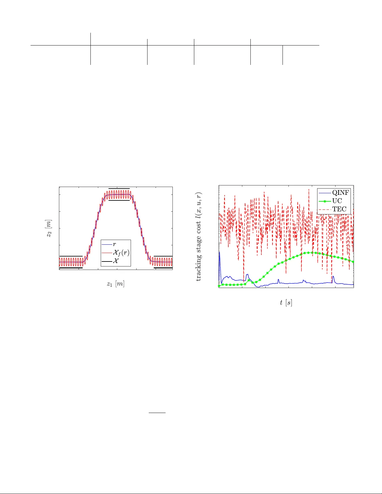
1 A nonlinear model predicti v e control frame work using reference generic terminal ingredients - e xtended version Johannes K ¨ ohler 1 , Matthias A. M ¨ uller 2 , Frank Allg ¨ ower 1 Abstract —In this paper , we present a quasi inﬁnite horizon nonlinear model predictive control (MPC) scheme for tracking of generic refer ence trajectories. This scheme is applicable to nonlinear systems, which are locally incrementally stabilizable. For such systems, we provide a reference generic ofﬂine pro- cedure to compute an incrementally stabilizing feedback with a continuously parameterized quadratic quasi inﬁnite horizon terminal cost. As a result we get a nonlinear r eference tracking MPC scheme with a valid terminal cost for general reachable refer ence trajectories without incr easing the online computational complexity . As a corollary , the terminal cost can also be used to design nonlinear MPC schemes that reliably operate under online changing conditions, including unreachable r eference signals. The practicality of this appr oach is demonstrated with a benchmark example. This paper is an extended version of the accepted paper [1], and contains additional details regarding robust trajectory track- ing (A pp. B), continuous-time dynamics (App. C), output tracking stage costs (App. D) and the connection to incremental system properties (App. A). Index T erms —Nonlinear model predictive contr ol, Constrained control, Reference tracking, Incremental Stability I . I N T RO D U C T I O N Model Predicti ve Control (MPC) [2] is a well established control method, that computes the control input by repeatedly solving an optimization problem online. The main adv antages of MPC are the ability to cope with general nonlinear dy- namics, hard state and input constraints, and the inclusion of performance criteria. In MPC (theory), recursiv e feasibility and closed-loop stability of a desirable setpoint are usually ensured by including suitable terminal ingredients (terminal set and terminal cost) in the optimization problem [3]. In man y applications, the control goal goes beyond the stabilization of a pre-determined setpoint. These practical challenges include tracking of changing reference setpoints, stabilization of dynamic trajectories, output regulation and general economic optimal operation. There exist many promis- ing ideas to tackle these issues in MPC, for example by simul- taneously optimizing an artiﬁcial reference [4], [5], [6], [7], 1 Johannes K ¨ ohler and Frank Allg ¨ ower are with the Institute for Systems Theory and Automatic Control, Univ ersity of Stuttgart, 70550 Stuttgart, Germany . (email: { johannes.koehler , frank.allgower } @ist.uni-stuttgart.de). 2 Matthias A. M ¨ uller is with the Institute of Automatic Control, Leibniz Univ ersity Hannov er , 30167 Hannov er , Germany . (email:mueller@irt.uni- hannover .de). Johannes K ¨ ohler would like to thank the German Research Foundation (DFG) for ﬁnancial support of the project within the International Research T raining Group Soft Tissue Robotics (GRK 2198/1 - 277536708). [8], [9], [10]. Howev er, most of these approaches are limited in some form to linear systems and/or setpoint stabilization. The computation of suitable terminal ingredients seems to be a bottleneck for the practical extension of these methods to nonlinear systems and dynamic trajectories. W e bridge this gap, by providing a reference generic ofﬂine computation for the terminal ingredients. Thus, we can provide practical schemes for nonlinear systems subject to changing operating conditions. Related work For linear stabilizable systems, a terminal set and terminal cost can be computed based on the linear quadratic regulator (LQR) and the maximal output admissible set [11]. For the purposes of stabilizing a gi ven setpoint, a suitable design pro- cedure for nonlinear systems with a stabilizable linearization has been provided in [12], [2]. In practice, the setpoint to be stabilized can change and thus procedures independent of the setpoint are necessary . In [13], the issue of ﬁnding a setpoint independent terminal cost has been inv estigated based on the concept of pseudo lin- earizations. While in principle v ery appealing, the computation of such a pseudo linearization for general nonlinear systems seems unpractical. In [14], a locally stabilizing controller is assumed and the terminal cost and constraints are deﬁned implicitly based on the inﬁnite horizon tail cost. The main drawback of this method is the implicit description of the terminal cost, which can signiﬁcantly increase the online com- putational demand. In [6] the feasible setpoints are partitioned into disjoint sets and for each such set a ﬁxed stabilizing controller and terminal cost are designed using the methods in [15], [16] based on a local linear time-v arying (L TV) system description. This method is mainly limited to systems with a one dimensional steady-state manifold, due to the otherwise complex and dif ﬁcult partitioning. In addition, the piece-wise deﬁnition can also lead to numerical dif ﬁculties since the terminal cost is not dif ferentiable with respect to the setpoint. There are man y applications in which we w ant to stabilize some dynamic trajectory or periodic orbit. The nonlinear system along this trajectory can be locally approximated with an L TV system. In [17], this is used to compute a (time- varying) terminal cost for asymptotically constant trajectories. In [18] periodic trajectories are considered and a (periodic) terminal cost is computed based on linear matrix inequalities c  2020 IEEE. Personal use of this material is permitted. Permission from IEEE must be obtained for all other uses, in any current or future media, including reprinting/republishing this material for advertising or promotional purposes, creating ne w collective works, for resale or redistrib ution to servers or lists, or reuse of any copyrighted component of this work in other works. 2 (LMIs). A signiﬁcant practical restriction for these methods is the f act that the ofﬂine computation is accomplished for a speciﬁc (a priori kno wn) trajectory . In general, the existing procedures to compute terminal in- gredients for MPC are mainly focused on computing a terminal cost for a speciﬁc reference point or reference trajectory . Thus, online changes in the setpoint or trajectory cannot be handled directly and necessitate repeated ofﬂine computations. Contribution In this work, we provide a reference generic ofﬂine pro- cedure to compute a parameterized terminal cost. This proce- dure is applicable to both setpoint or trajectory stabilization. The feasibility of this approach requires local incremental stabilizability of the nonlinear dynamics. The existing design procedures [12], [17], [18] use the linearization around the considered setpoint or trajectory to locally establish properties of the nonlinear systems. In a similar spirit, we consider the linearization of the nonlinear system dynamics around all possible points in the constraint set and describe the dynamics analogous to quasi-linear parameter-v arying (LPV) systems. W ith this description, we formulate the desired properties on the linearized dynamics and provide suitable LMIs to compute the parameter dependent terminal cost and controller . In closed-loop operation we hav e a quadratic terminal cost with an ellipsoidal terminal constraint directly available. This provides a generalization of the of ﬂine computations in [12], [17], [18] to generic references. W e employ the proposed method in an ev asive maneuver test for a car and show that the design of suitable reference generic terminal ingredients can signiﬁcantly improve the control performance compared to MPC schemes with terminal equality constraints or without terminal constraints. Giv en these terminal ingredients, we can extend existing tracking MPC schemes, such as [4], [5], [6], [7], [8], [9], [10] to nonlinear system dynamics and optimal periodic operation, which is a fundamental step to wards practical nonlinear MPC schemes. In particular , we provide a nonlinear periodic track- ing MPC scheme for exogenous output signals as an extension to [4], [5], [6]. Outline The remainder of this paper is structured as follo ws: Sec- tion II presents the reference tracking MPC scheme based on the proposed parameterized terminal ingredients. Section III provides a constructive procedure to design parametric ter- minal ingredients independent of the considered reference. Section IV shows how the resulting parameterized terminal ingredients can be used to e xtend e xisting MPC schemes for changing operation conditions to nonlinear system dynamics and periodic operation. Section V shows the practicality of this procedure with numerical examples. Section VI concludes the paper . In the appendix, these results are extended to r obust trajectory tracking (App. B), continuous-time dynamics (App. C), and output tracking stage costs (App. D). In addition, the connection between the generic terminal ingredients and incremental system properties is discussed (App. A). I I . R E F E R E N C E T R AC K I N G M O D E L P R E D I C T I V E C O N T RO L A. Notation The quadratic norm with respect to a positi ve deﬁnite matrix Q = Q > is denoted by k x k 2 Q = x > Qx . The minimal and maximal eigen value of a symmetric matrix Q = Q > is denoted by λ min ( Q ) and λ max ( Q ) , respectiv ely . The identity matrix is I n ∈ R n × n . The interior of a set X is denoted by int ( X ) . The vertices of a polytopic set Θ are denoted by θ i ∈ V ert (Θ) . B. Setup W e consider the follo wing nonlinear discrete-time system x ( t + 1) = f ( x ( t ) , u ( t )) (1) with the state x ∈ R n , control input u ∈ R m , and time step t ∈ N . The extension of the following deriv ation to continuous- time dynamics is detailed in Appendix C. W e impose point- wise in time constraints on the state and input ( x ( t ) , u ( t )) ∈ Z , (2) with some compact 1 set Z . W e consider the following assump- tion regarding the reference signal r = ( x r , u r ) ∈ R n + m . Assumption 1. The r efer ence signal r satisﬁes r ( t ) ∈ Z r , ∀ t ≥ 0 , with some set Z r ⊆ int ( Z ) . Furthermor e, the e volution of the r eference signal is r estricted by r ( t + 1) ∈ R ( r ( t )) , with R ( r ) = { ( x + r , u + r ) ∈ Z r | x + r = f ( x r , u r ) } . This assumption characterizes that the reference trajectory r is reachable, i.e., follows the dynamics f and lies (strictly) in the constraint set Z . If the reference trajectory is not reachable it is possible to enforce these constraints on an artiﬁcial reference trajectory which can be included in the MPC optimization problem, compare Section IV. Remark 1. The set R ( r ) can be modiﬁed to incorporate addi- tional incremental input constraints k u r ( t + 1) − u r ( t ) k ∞ ≤  . Setpoints ar e included as a special case, with R ( r ) = r and the steady-state manifold Z r . C. T erminal cost and terminal set Denote the tracking error by e r ( t ) = x ( t ) − x r ( t ) . The control goal is to stabilize the tracking error e r ( t ) = 0 and achiev e constraint satisfaction ( x ( t ) , u ( t )) ∈ Z , ∀ t ≥ 0 . T o this end we deﬁne the quadratic reference tracking stage cost ` ( x, u, r ) = k x − x r k 2 Q + k u − u r k 2 R , (3) with positiv e deﬁnite weighting matrices Q, R . Remark 2. The extension to an trac king stage cost ` ( x, u, r ) = k h ( x, u ) − h ( x r , u r ) k 2 S ( r ) with some output y = h ( x, u ) and a positive deﬁnite weighting matrix S is discussed in the Appendix D. As discussed in the introduction, we need suitable terminal ingredients to ensure stability and recursi ve feasibility for the closed-loop system. 1 The deriv ations can be extended to time-v arying constraint sets Z ( t ) and dynamics f ( x, u, t ) . The consideration of non-compact constraint sets may require additional uniformity conditions on the nonlinear dynamics. 3 Assumption 2. There exist matrices K f ( r ) ∈ R m × n , P f ( r ) ∈ R n × n with c l I n ≤ P f ( r ) ≤ c u I n , a terminal set X f ( r ) = { x ∈ R n | V f ( x, r ) ≤ α } with the terminal cost V f ( x, r ) = k x − x r k 2 P f ( r ) , such that the following pr operties hold for any r ∈ Z r , any x ∈ X f ( r ) and any r + ∈ R ( r ) V f ( x + , r + ) ≤ V f ( x, r ) − ` ( x, k f ( x, r ) , r ) , (4a) ( x, k f ( x, r )) ∈Z , (4b) with x + = f ( x, k f ( x, r )) , k f ( x, r ) = u r + K f ( r ) · ( x − x r ) and positive constants c l , c u , α . For r = r + = 0 this reduces to the standard conditions in [12]. For a given trajectory r , this implies time-varying terminal ingredients, compare [17], [18]. Designing suitable 2 terminal ingredients that satisfy this assumption is the main contribution of this paper and is discussed in more detail in the Section III. Remark 3. Assumption 1 implies that the r efer ence r ( t ) is contained within a contr ol in variant subset Z ∞ ⊆ Z r . Thus, Assumption 2 could be relaxed, such that the conditions (4) only need to be satisﬁed for points r ∈ Z ∞ . The exact char acterization of the set Z ∞ is, however , challenging and thus we consider the stricter 3 conditions as formulated in Assumption 2. D. Pr eliminary r esults Denote the reference r o ver the prediction horizon N by r ( ·| t ) ∈ R ( n + m ) × ( N +1) with r ( k | t ) = r ( t + k ) , k = 0 , . . . , N . Given a predicted state and input sequence x ( ·| t ) ∈ R n × N +1 , u ( ·| t ) ∈ R m × N the tracking cost with respect to the reference r ( ·| t ) is gi ven by J N ( x ( ·| t ) , u ( ·| t ) , r ( ·| t )) := N − 1 X k =0 ` ( x ( k | t ) , u ( k | t ) , r ( k | t )) + V f ( x ( N | ) , r ( N | t )) . The MPC scheme is based on the follo wing (standard) MPC optimization problem V ( x ( t ) , r ( ·| t )) = min u ( ·| t ) J N ( x ( ·| t ) , u ( ·| t ) , r ( ·| t )) (5a) s.t. x ( k + 1 | t ) = f ( x ( k | t ) , u ( k | t )) , (5b) x (0 | t ) = x ( t ) , (5c) ( x ( k | t ) , u ( k | t )) ∈ Z , (5d) x ( N | t ) ∈ X f ( r ( N | t )) . (5e) The solution to this optimization problem are the value func- tion V and the optimal input trajectory u ∗ ( ·| t ) . In closed- 2 In principle, this assumption can always be satisﬁed with a terminal equality constraint X f ( r ) = x r . Howe ver , this can lead to numerical problems, and decrease performance and robustness of the MPC scheme. In addition, tracking schemes such as [4], [6], [19], typically require a non-vanishing terminal set size α to ensure exponential stability , compare Section IV. 3 If there exists a ﬁxed constant T 0 , such that r ( t + k ) ∈ Z r , ∀ k ∈ [0 , T 0 ] , implies r ( t ) ∈ Z ∞ , then the conditions in Assumption 2 are not stricter . Howe ver, if we use a con ve x overapproximation (Prop. 1) and/or parameterize the matrices P f , K f , then this may introduce additional conservatism. loop operation we apply the ﬁrst part of the optimized input trajectory to the system, leading to the follo wing closed loop x ( t + 1) = f ( x ( t ) , u ∗ (0 | t )) = x ∗ (1 | t ) , t ≥ 0 . (6) The following theorem summarizes the standard theoretical properties of the closed-loop system (6). Theorem 1. Let Assumptions 1 and 2 hold. Assume that Pr oblem (5) is feasible at t = 0 . Then Pr oblem (5) is r e- cursively feasible and the tracking err or e r = 0 is (uniformly) exponentially stable for the r esulting closed-loop system (6) . Pr oof. This theorem is a straight forw ard e xtension of standard MPC results in [20], compare also [17]. Given the optimal solution u ∗ ( ·| t ) , the candidate sequence u ( k | t + 1) = ( u ∗ ( k + 1 | t ) k ≤ N − 2 k f ( x ∗ ( N | t ) , r ( N | t )) k = N − 1 , (7) is a feasible solution to (5a) and implies V ( x ( t + 1) , r ( ·| t + 1)) ≤ V ( x ( t ) , r ( ·| t )) − ` ( x ( t ) , u ( t ) , r ( t )) . (8) Compact constraints in combination with the quadratic termi- nal cost imply k x ( t ) − x r ( t ) k 2 Q ≤ V ( x ( t ) , r ( ·| t )) ≤ c v k x ( t ) − x r ( t ) k 2 Q , for some c v ≥ 1 . Uniform exponential stability follows from standard L yapunov arguments using the v alue function V . This theorem shows that if we can design suitable terminal ingredients (Ass. 2), the closed-loop tracking MPC has all the (standard) desirable properties. In Section IV we discuss how this can be extended to more general tracking problems. This scheme can be easily modiﬁed to ensure robust reference tracking using the method in [21], for details see Appendix B and the numerical example in Section V. Remark 4. A powerful alternative to the pr oposed quasi- inﬁnite horizon refer ence tracking MPC scheme would be a r eference trac king MPC scheme without terminal ingr edi- ents [22] ( V f ( x, r ) = 0 , X f ( r ) = X ). If it is possible to design terminal ingr edients (Ass. 2), the value function of such an MPC scheme without terminal constraints is locally bounded by V ( x ( t ) , r ( ·| t )) ≤ γ ` ( x, u, r ) , with a suitable constant γ , compare [22, Prop. 2]. Thus, an MPC scheme without terminal constraints enjoys similar closed-loop pr operties to Theor em 1, pr ovided a sufﬁciently large pr ediction horizon N is used, compare [22, Thm. 2]. One of the core advantages of including suitably designed terminal ingr edients is that we can implement the MPC scheme with a short pr ediction horizon N . On the other hand, if the refer ence is not reac hable (Ass. 1), MPC schemes without terminal constr aints can still be successfully applied [22, Thm. 4], which is in gener al not the case for MPC schemes with terminal constraints. I I I . R E F E R E N C E G E N E R I C O FFL I N E C O M P U T AT I O N S This section provides a reference generic ofﬂine compu- tation to design terminal ingredients for nonlinear reference tracking MPC. In Lemma 1 we provide sufﬁcient conditions 4 for the terminal ingredients based on properties of the lin- earization. Then, two approaches based on LMI computations are described to compute the terminal ingredients, based on Lemma 2 and Proposition 1. After that, a procedure to obtain a non conserv ativ e terminal set size α is discussed. Finally , the overall ofﬂine procedure is summarized in Algorithm 2. For the special case of setpoint tracking, existing methods are discussed in relation to the proposed procedure. In Appendix C and D, these results are extended to continuous-time dynamics and output tracking stage costs, respectively . A. Sufﬁcient conditions based on the linearization W e denote the Jacobian of f ev aluated around an arbitrary point r ∈ Z r by A ( r ) =  ∂ f ∂ x      ( x,u )= r , B ( r ) =  ∂ f ∂ u      ( x,u )= r . (9) The following lemma establishes local incremental properties of the nonlinear system dynamics based on the linearization. Lemma 1. Suppose that f is twice continuously differ entiable. Assume that ther e e xists a matrix K f ( r ) ∈ R m × n and a positive deﬁnite matrix P f ( r ) ∈ R n × n continuous in r , such that for any r ∈ Z r , r + ∈ R ( r ) , the following matrix inequality is satisﬁed ( A ( r ) + B ( r ) K f ( r )) > P f ( r + )( A ( r ) + B ( r ) K f ( r )) (10) ≤ P f ( r ) − ( Q + K f ( r ) > RK f ( r )) − I n with some positive constant  . Then ther e e xists a sufﬁciently small constant α , such that P f , K f satisfy Assumption 2. Pr oof. The proof is very much in line with the result for setpoints in [12], [2]. First we sho w satisfaction of the decrease condition (4a) and then constraint satisfaction (4b). Part I: Denote ∆ x := x − x r and ∆ u := K f ( r )∆ x . Using a ﬁrst order T aylor approximation at r = ( x r , u r ) , we get f ( x, k f ( x, r )) = f ( x r , u r ) + A ( r )∆ x + B ( r )∆ u + Φ r (∆ x ) , with the remainder term Φ r . The terminal cost satisﬁes V f ( x + , r + ) = k f ( x, u ) − f ( x r , u r ) k 2 P f ( r + ) = k ( A ( r ) + B ( r ) K f ( r ))∆ x + Φ r (∆ x ) k 2 P f ( r + ) ≤k ( A ( r ) + B ( r ) K f ( r ))∆ x k 2 P f ( r + ) + k Φ r (∆ x ) k 2 P f ( r + ) + 2 k Φ r (∆ x ) k P f ( r + ) k ( A ( r ) + B ( r ) K f ( r ))∆ x k P f ( r + ) (10) ≤ V f ( x, r ) −  k ∆ x k 2 − ` ( x, k f ( x, r ) , r ) + k Φ r (∆ x ) k 2 P f ( r + ) + 2 k Φ r (∆ x ) k P f ( r + ) k ( A ( r ) + B ( r ) K f ( r ))∆ x k P f ( r + ) . (11) Using the continuity of P f ( r ) , K f ( r ) and the compactness of the constraint set Z r , there exist ﬁnite constants c u = max r ∈Z r λ max ( P f ( r )) , c l = min r ∈Z r λ min ( P f ( r )) , (12) k u = max r ∈Z r k K f ( r ) k , (13) c u, 2 = max r ∈Z r λ max ( P f ( r ) − ( I + Q + K f ( r ) > RK f ( r ))) . Suppose that the remainder term Φ r is locally Lipschitz 4 continuous in the terminal set with a constant L Φ ,α satisfying k Φ r (∆ x ) k ≤ L Φ ,α k ∆ x k , L Φ ,α ≤ L ∗ Φ := r c u, 2 +  c u − r c u, 2 c u . (14) Then we have k Φ r (∆ x ) k 2 P f ( r + ) + 2 k Φ r (∆ x ) k P f ( r + ) k ( A ( r ) + B ( r ) K f ( r ))∆ x k P f ( r + ) (10)(12)(14) ≤  L 2 Φ ,α c u + 2 L Φ ,α √ c u √ c u, 2  k ∆ x k 2 = c u  L Φ ,α + r c u, 2 c u  2 − c u, 2 ! k ∆ x k 2 (14) ≤  k ∆ x k 2 , which in combination with (11) implies the desired inequal- ity (4a). T wice continuous differentiability of f in combination with compactness of Z implies that there e xists some constant T with k Φ r (∆ x ) k ≤ T  k ∆ x k 2 + k ∆ u k 2  (13) ≤ T (1 + k 2 u ) k ∆ x k 2 . Using k ∆ x k ≤ q α c l from the terminal constraint, we get (14) for all α ≤ α 1 with α 1 := c l  L ∗ Φ T (1 + k 2 u )  2 . (15) Part II: Constraint satisfaction: The terminal constraint k ∆ x k 2 P f ( r ) ≤ α in combination with (12), (13) implies (∆ x, ∆ u ) ∈ B ( α ) =  z ∈ R n + m | k z k 2 ≤ α c l  1 + k 2 u   . Giv en Z r ⊆ Int ( Z ) , there e xists a small enough α 2 such that ( x, u ) = r + (∆ x, ∆ u ) ⊆ Z r ⊕ B ( α ) ⊆ Z , ∀ α ≤ α 2 . (16) As a summary , gi ven matrices P f , K f satisfying (10), we can compute a local Lipschitz bound (14), which in turn im- plies a maximal terminal set size α 1 . Similarly , the constraint sets Z and Z r in combination with K f , P f imply an upper bound α 2 to ensure constraint satisfaction. Then Assumption 2 is satisﬁed for any α ≤ min { α 1 , α 2 } . This result is an extension of [12], [2] to arbitrary dynamic references. B. Quasi-LPV based procedur e Lemma 1 states that matrices satisfying inequality (10) also satisfy Assumption 2 with a suitable terminal set size α . In the following, we formulate computationally tractable optimization problems to compute matrices that satisfy the conditions in Lemma 1. The following Lemma transforms the conditions in (10) to be linear in the arguments. 4 In line with existing procedures [12], we ﬁrst deriving a sufﬁcient local Lipschitz bound L ∗ Φ and then obtain a local region α 1 (15). Alternatively , it is possible to directly use the quadratic bound k Φ r (∆ x ) k ≤ c k ∆ x k 2 and work with higher order terms to obtain α 1 , compare [22, Prop. 1]. 5 Lemma 2. Suppose that ther e exists matrices X ( r ) , Y ( r ) continuous in r , that satisfy the constraints in (19) for all r ∈ Z r , r + ∈ R ( r ) . Then P f = X − 1 , K f = Y P f satisfy (10) . Pr oof. The proof is standard, compare [23] and Lemma 6 in the Appendix. The optimization problem (19) is con ve x, linear in X , Y and minimizes the worst-case terminal cost P f ( r ) ≤ X − 1 min . So far , the result is only conceptual, since (19) is an inﬁ- nite programming problem (inﬁnite dimensional optimization variables with inﬁnite dimensional constraints). In particular , we need a ﬁnite parameterization of X , Y and the inﬁnite constraints need to be conv erted into a ﬁnite set of suf ﬁcient constraints. Remark 5. One solution to this pr oblem would be sum- of-squar es (SOS) optimization [24]. Assuming A, B are polynomial, consider matrices X , Y polynomial in r (with a speciﬁed or der d ) and ensure that the matrix in (19) is SOS. A similar appr oach is suggested in [25] to ﬁnd a contr ol contraction metric (CCM) for continuous-time systems (which is a str ongly related pr oblem). This appr oach is not pursued her e since most systems requir e a polynomial of high order to appr oximate the nonlinear dynamics and the computational complexity gr ows e xponentially in n d , thus pr ohibiting the practical application. The connection between CCM and LPV gain-scheduling design is discussed in [26]. W e approach this problem from the perspective of quasi- LPV systems and gain-scheduling [27]. First, write the Jaco- bian (9) as A ( r ) = A 0 + p X j =1 θ j ( r ) A j , B ( r ) = B 0 + p X j =1 θ j ( r ) B j , (17) with some nonlinear (continuously differentiable) parameters θ ∈ R p . This can always be achie ved with p ≤ n ( n + m ) . W e impose the same structure on the optimization v ariables with X ( r ) = X 0 + p X j =1 θ j ( r ) X j , Y ( r ) = Y 0 + p X j =1 θ j ( r ) Y j . (18) Remark 6. F or input afﬁne systems of the form f ( x, u ) = f x ( x ) + B u , the Jacobian (17) and corr espondingly the parameters θ i only depend on x r . Thus, the r esulting terminal ingr edients ar e solely par ameterized by the state x r . Using the parameterization (17)-(18), (19) contains only a ﬁnite number of optimization variables, b ut still needs to be veriﬁed for all r ∈ Z r , r + ∈ R ( r ) . There are two options to deal with this: con vexifying the problem or gridding the constraint set. 1) Con vexify: In order to conv exify (19), we match the constraint sets Z r , R ( r ) on the reference r to polytopic constraint sets Θ , Ω on the parameters θ . The polytopic sets Θ , Ω( θ ) need to satisfy θ ( r ) ∈ Θ , ∀ r ∈ Z r , (21) θ ( r + ) ∈ Ω( θ ( r )) , ∀ r + ∈ R ( r ) . Computing a set Θ , such that θ ( r ) ∈ Θ for all r ∈ Z r can be achieved by considering a hyperbox Θ = { θ ∈ R p | θ i ∈ [ θ i , θ i ] } . F or Ω , a simple approach is Ω( θ ) = { θ } ⊕ Ω , where Ω is a hyperbox that encompasses the maximal change in the parameters θ in one time step, i.e. Ω = { ∆ θ ∈ R p | ∆ θ i ∈ [ v i , v i ] } . W e denote the joint polytopic constraint set by ( θ , θ + ) ∈ Θ = { ( θ , θ + ) ∈ Θ × Θ | θ + ∈ { θ } ⊕ Ω } , (22) which consists of 6 p vertices. The following proposition provides a simple con ve x procedure to compute a terminal cost, by solving a ﬁnite number of LMIs. Proposition 1. Suppose that ther e exist matrices X i , Y i , Λ i , X min that satisfy the constraints in (20) . Then the matrices P f ( r ) = X − 1 ( r ) , K f ( r ) = Y ( r ) P f ( r ) , satisfy (10) , with X, Y accor ding to (18) . Pr oof. Due to Lemma 2, it suf ﬁces to show that X ( r ) , Y ( r ) satisfy the constraints in (19). Due to the deﬁnition of the set Θ (22) and Λ i ≥ 0 , any solution that satisﬁes the constraints (20b) over all ( θ , θ + ) ∈ Θ , also satisﬁes the constraints (19) for all r ∈ Z r , r + ∈ R ( r ) . It remains to show that it sufﬁces to check the inequality on the vertices of the constraint set Θ . This last result is a consequence of multi- con vexity [28, Corollary 3.2]. In particular , if a function f is multi-concav e along the edges of the constraint set Θ , then it attains its minimum at a vertex of Θ and thus it sufﬁces to verify (20b) ov er the vertices of Θ . The edges of Θ (22) are characterized by { θ i , θ + i , θ + i − θ i } , i = 1 , . . . , p . A function is multi-concav e if the second deriv ative w .r .t. these directions is negati ve-semi-deﬁnite, compare [28, Corollary 3.4]. Similar to [28, Corollary 3.5], the additional constraint (20d) ensures that the function is multi-concav e. Thus, it sufﬁces to verify inequality (20b) on the vertices of the constraint set Θ . Remark 7. The r esult in Proposition 1 r emains valid, if the set Θ in (22) is r eplaced by the set Θ = Θ × (Θ ⊕ Ω) . This set has only 4 p vertices and the induced conservatism of this appr oximation is ne gligible if Ω is small compar ed to Θ . 2) Gridding: A common heuristic to ensure that parameter dependent LMIs such as (19) hold for all ( r , r + ) is to consider the constraints on sufﬁciently many sample points in the constraint set, compare e.g. [28, Sec. 4.2]. Due to continuity , the constraint is typically satisﬁed on the full constraint set if it holds on a sufﬁciently ﬁne grid. For this method it is crucial that satisfaction of (4a) is v eriﬁed by using a ﬁne grid (compare Algorithm 1). The gridding consists of a grid ov er all possible state and input combinations ( r, r + ) , i.e., all considered points satisfy r , r + ∈ Z r , r + ∈ R ( r ) , R ( r + ) 6 = ∅ . (23) For the simple structure R ( r ) in Assumption 1 this can be achiev ed by gridding r , computing x + r = f ( x r , u r ) , and considering all u + r , such that ( x + r , u + r ) ∈ Z r and ( f ( x + r , u + r ) , ˜ u r ) ∈ Z r with some ˜ u r . This approach does not introduce additional conservatism, but is computationally 6 min X ( r ) ,Y ( r ) ,X min − log det X min (19a) s.t.     X ( r ) X ( r ) A ( r ) > + Y ( r ) > B ( r ) > ( Q +  ) 1 / 2 X ( r ) ( R 1 / 2 Y ( r )) > ∗ X ( r + ) 0 0 ∗ ∗ I 0 ∗ ∗ ∗ I     ≥ 0 , (19b) X min ≤ X ( r ) , (19c) ∀ r ∈ Z r , r + ∈ R ( r ) . (19d) min X i ,Y i , Λ i ,X min − log det X min (20a) s.t.     X ( θ ) X ( θ ) A ( θ ) > + Y ( θ ) > B ( θ ) > ( Q +  ) 1 / 2 X ( θ ) ( R 1 / 2 Y ( θ )) > ∗ X ( θ + ) 0 0 ∗ ∗ I 0 ∗ ∗ ∗ I     −  P p i =1 θ 2 i Λ i 0 0 0  ≥ 0 , (20b) X min ≤ X ( θ ) , ∀ ( θ , θ + ) ∈ V ert (Θ) , (20c)  0 ( A i X i + B i Y i ) > ( A i X i + B i Y i ) 0  − Λ i ≤ 0 , Λ i ≥ 0 , i = 1 , . . . , p. (20d) challenging for high dimensional systems. As discussed in Re- mark 1 we can include additional constraints on the reference, which makes the ofﬂine computation less conserv ativ e. If some parameters, e.g. u r , enter the LMIs afﬁnely and are subject to polytopic constraints, it sufﬁces to consider the vertices of the corresponding constraint set. The advantage of the conv ex procedure (compared to the gridding) is that it typically scales better with the system dimension. This comes at the cost of additional conservatism due to the construction of the set Θ and the additional multi- con vexity constraint (20d). The computational demand can be reduced by considering (block-)diagonal multipliers Λ i = λ i I . It can often be beneﬁcial to consider a combination of the two approaches, i.e. grid in some dimensions and conserv ativ ely con vexify in others. The adv antages and applicability of both approaches are explored in more detail in the numerical examples in Section V. The main result is that we can formulate the ofﬂine design procedure similar to the gain scheduling synthesis of (quasi)- LPV systems and thus can draw on a well established ﬁeld to formulate 5 ofﬂine LMI procedures, compare [27]. C. Non-conservative terminal set size α The terminal set size α deri ved in Lemma 1 can be quite conserv ativ e. In the follo wing we illustrate how a non conservati ve value α can be computed (giv en P f and K f ). 1) Constraint satisfaction - α 2 : Assume that we have polytopic constraints of the form Z = { r = ( x, u ) | L r r ≤ l } . 5 If the parameters θ i are chosen based on a vertex representation ( θ i ≥ 0 , P p i =1 θ i = 1 ) the multi-con vexity condition (20d) can be replaced by positivity conditions of the polynomials, compare for example [29]. In [30] a conve xiﬁcation with an additional matrix is considered. More elaborate methods to formulate LPV synthesis with ﬁnite LMIs can be found in [31]. The constant α 2 , with the property that α ≤ α 2 implies constraint satisfaction (4b), can be computed with α 2 := max α α (24) s.t. k P f ( r ) − 1 / 2  I n K > f ( r )  L > r,j k 2 α ≤ ( l j − L r,j r ) 2 , ∀ r ∈ Z r , j = 1 , . . . n z . This problem can be efﬁciently solved by girdding the con- straint set Z r , solving the resulting linear program (LP) for each point r and taking the minimum. In the special case that P f , K f are constant this reduces to one small scale LP . 2) Local Stability - α 1 : Determining a non-conservati ve constant α 1 , related to the local L yapunov function V f can be signiﬁcantly more difﬁcult. For comparison, in the setpoint stabilization case a non-conv ex optimization problem is for- mulated to check whether (4a) holds for a speciﬁc value of α 1 , compare [12, Rk. 3.1]. In a similar fashion, we consider the following algorithm 6 to determine whether (4a) holds for all α ≤ α 1 : Algorithm 1 Ofﬂine computation - Local stability α 1 Giv en a candidate constant α 1 : Grid: Select ( r , r + ) satisfying (23) 1: Ev aluate P f ( r ) , P f ( r + ) , K f ( r ) using (18). 2: Generate random vectors ∆ x i : with k ∆ x i k 2 P f ( r ) ≤ α 1 . 3: Check if x i = x r + ∆ x i satisﬁes (4a). Starting with α 1 = α 2 , the value α 1 is iterativ ely decreased until all considered combination ( r , r + , x i ) satisfy (4a). The overall of ﬂine procedure to compute the terminal in- gredients (Ass. 2) is summarized as follo ws: 6 Algorithm 1 can be thought of as a sampling based strategy to solve this non-con vex optimization problem considered in [12, Rk. 3.1]. Using standard conv ex solvers, like sequential quadratic programming (SQP), yield a faster solution, but can get stuck in local minima. This is dangerous for this problem, since the local minima correspond to values α that do not satisfy Assumption 2. Alternativ ely , nonlinear Lipschitz-like bounds can be used to reduce the conservatism, compare [32] (which, howev er, also use sampling). 7 Algorithm 2 Ofﬂine computation 1: Deﬁne θ corresponding to the linearization (17). 2: LMI computation using gridding or con ve xiﬁcation: Con vex : Determine hyperbox sets Θ , Ω satisfying (21). Solve (20) using Θ according to (22) or Remark 7. Gridding : Select ( r i , r + i ) satisfying (23). Solve (19) for all ( r i , r + i ) . 3: Compute size of the terminal set α = min { α 1 , α 2 } : a):compute α 1 using Algorithm 1 (or (15)), b):compute α 2 using (24) (or (16)). The presented ofﬂine procedure is considerably more in- volv ed than for example the computation for one speciﬁc setpoint [12]. W e emphasize that this procedure only has to be completed once and we need no repeated ofﬂine computations to account for changing operation conditions. Furthermore, the applicability to nonlinear systems with the corresponding com- putational effort ofﬂine is detailed with numerical examples in Section V. D. Setpoint trac king Now we discuss setpoint tracking, which is included in the previous deriv ation as a special case with Z r such that ( x r , u r ) ∈ Z r implies x r = f ( x r , u r ) and R ( r ) = r . Note, that both presented approaches signiﬁcantly simplify in this case. For the gridding approach it sufﬁces to grid along the steady-state manifold Z r which is typically low dimensional. In the con ve x approach (Prop. 1) we hav e θ + = θ and thus we only consider the 2 p vertices of Θ . Compared to the dynamic reference tracking problem, the problem of tracking a setpoint has receiv ed a lot of attention in the literature and many solutions have been suggested. One of the ﬁrst attempts to solve this issue is the usage of a pseudo linearization in [13]. There, a nonlinear state and input transformation is sought, such that the linearization of the transformed system around the setpoints is constant and thus constant terminal ingredients can be used. This approach seems unpractical, since there is no easy or simple method to compute such a pseudo linearization. In [6], [15], [16] the steady-state manifold Z r is partitioned into sets. In each set the nonlinear system is described as an L TV system and a constant terminal cost and controller are computed. Correspondingly , in closed-loop operation under changing setpoints [6] the terminal cost matrix P f is piece- wise constant. This might cause numerical problems in the optimization, since the cost is not differentiable with respect to the reference r . Furthermore, the (manual) partitioning of the steady-state manifold seems difﬁcult for general MIMO systems (if the dimension of the steady-state manifold is larger than one). In comparison, Algorithm 2 yields continuously parameterized terminal ingredients, thus av oiding the need for user deﬁned partitioning and piece-wise deﬁnitions. In [9, Remark 8] it was proposed to compute a continuously parameterized controller K f ( r ) by analytically using a pole- placement formula and solving the corresponding L yapunov 7 equation to obtain P f ( r ) . The resulting terminal ingredients are quite similar to the proposed ones. Howe ver , this proce- dure cannot be directly translated into a simple optimization problem and might hence not be tractable. I V . N O N L I N E A R M P C S U B J E C T T O C H A N G I N G O P E R AT I O N C O N D I T I O N S Many control problems are more general than the reference tracking considered in Section II. One challenge includes tracking and output regulation with exogenous signals in order to accommodate online changing operation conditions. F or this set of problems, the reference r might not satisfy Assumption 1 (due to sudden changes and unreachable signals), compare [4], [5], [6]. More generally , the minimization of a possibly online changing and non-con vex economic cost is a (non-trivial) control problem which is often encountered, compare [7], [8], [9], [10]. One promising method to solve these problems is the simultaneous optimization of an artiﬁcial reference, as done in [4], [5], [6], [7], [8], [9], [10]. Compared to a standard reference tracking MPC formulation such as (5), these schemes ensure recursi ve feasibility despite changes in exogenous signals (such as the desired output reference or the economic cost). In this section, we show how the reference generic terminal ingredients can be used to design nonlinear MPC schemes that reliably operate under changing operating conditions, as an extension and combination of the ideas in [4], [5], [6], [7], [8], [9], [10]. In particular, we present a scheme that exponentially stabilizes the periodic trajectory which best tracks an exogenous output signal. The e xtension of the economic MPC schemes [7], [8], [9], [10] to periodic artiﬁcial trajectories based on the reference generic terminal ingredients is be yond the scope of this work and part of current research. A. Nonlinear periodic tracking MPC subject to changing exo genous output refer ences W e assume that at time t an exogenous T -periodic output reference signal y e ( ·| t ) ∈ R p × T is given. For some T -periodic reference r ( ·| t ) = ( x r ( ·| t ) , u r ( ·| t )) ∈ R ( n + m ) × T , we deﬁne the tracking cost with respect to this output signal y e by J T ( r ( ·| t ) , y e ( ·| t )) = T − 1 X j =0 k h ( r ( j | t )) | {z } = y r ( j | t ) − y e ( j | t ) k 2 , with a bounded nonlinear output function h : Z r → R p . The objective is to stabilize the feasible T -periodic reference trajectory r , that minimizes J T . In [4], [6] the issue of stabilizing the optimal setpoint for piece-wise constant output signals has been in vestigated. In [5] periodic trajectories have been considered for the special case of linear systems. By 7 In [9], the terminal cost V f is computed for a (differentiable) economic stage cost ` ( x, u ) (not necessarily quadratic), compare also [7]. The compu- tation of the terminal cost is decomposed into a linear and quadratic term, compare [33]. Computing the quadratic term of this economic terminal cost is equiv alent to computing a quadratic terminal cost for a quadratic stage cost (Ass 2). 8 combining these methods with the proposed terminal ingredi- ents, we can design a nonlinear MPC scheme that stabilizes the optimal periodic 8 trajectory for periodic output reference signals, compare [19]. The scheme is based on the following optimization problem W T ( x ( t ) , y e ( ·| t )) (25a) = min u ( ·| t ) ,r ( ·| t ) J N ( x ( ·| t ) , u ( ·| t ) , r ( ·| t )) + J T ( r ( ·| t ) , y e ( ·| t )) s.t. x ( k + 1 | t ) = f ( x ( k | t ) , u ( k | t )) , x (0 | t ) = x ( t ) , (25b) ( x ( k | t ) , u ( k | t )) ∈ Z , x ( N | t ) ∈ X f ( r ( N | t )) , (25c) r ( j + 1 | t ) ∈ R ( r ( j | t )) ⊆ Z r , (25d) r ( l + T | t ) = r ( l | t ) , l = 0 , . . . , max { 0 , N − T } , (25e) j = 0 , . . . , T − 1 , k = 0 , . . . , N − 1 . This scheme is recursiv ely feasible, independent of the output reference signal y e . Furthermore, if the exogenous signal y e is T -periodic the closed-loop system is stable. Additionally , if a con ve xity and continuity condition on the set of feasible periodic orbits and the output function h is satisﬁed [19, Ass. 5], then the optimal reachable periodic trajectory is (uniformly) e xponentially stable for the resulting closed-loop system. Thus, the terminal ingredients enable us to implement a nonlinear version of the tracking scheme in [4], [5], that ensures exponential stability of the optimal (periodic) opera- tion. More details on the theoretical properties and numerical examples can be found in [19]. Although the consideration of general non-periodic trajectories is still an open issue, we conjecture that the approach can be e xtended to any class of ﬁnitely parameterized reference trajectories. V . N U M E R I C A L E X A M P L E S The follo wing examples sho w the applicability of the pro- posed method to nonlinear systems and the closed-loop perfor- mance improv ement when including suitable terminal ingredi- ents. W e ﬁrst illustrate the basic procedure at the example of a periodic reference tracking task for a continuous stirred-tank reactor (CSTR). Then we demonstrate the adv antages of using suitable terminal ingredients with (rob ust) trajectory tracking and an ev asiv e maneuv er test for a car . Additional examples, including tracking of periodic output signals (Sec. IV -A) with a nonlinear ball and plate system can be found in [19]. In the follo wing examples, the ofﬂine computation is done with an Intel Core i7 using the semideﬁnite programming (SDP) solver SeDuMi-1.3 [34] and the online optimization is done with CasADi [35]. The ofﬂine computation can be done using both the discrete-time formulation (Sec. III) or the continuous-time formulation (Appendix C). Hence, we also compare the performance of these different formulations. 8 In the case of setpoint tracking ( T = 1 ), the MPC scheme reduces to [6]. As discussed in Section III-D, the proposed procedure can be used to design suitable terminal ingredients for setpoints. A. P eriodic refer ence tracking - CSTR System model: W e consider a continuous-time model of a continuous stirred-tank reactor (CSTR)   ˙ x 1 ˙ x 2 ˙ x 3   =   1 − x 1 − 10 4 x 2 1 exp( − 1 x 3 ) − 400 x 1 exp( − 0 . 55 x 3 ) 10 4 x 2 1 exp( − 1 x 3 ) − x 2 u − x 3   , where x 1 , x 2 , x 3 correspond to the concentration of the reaction, the desired product, waste product and u is related to the heat ﬂux through the cooling jacket, compare [36], [37, Sec. 3.4]. The constraints are Z r =[0 . 05 , 0 . 45] × [0 . 05 , 0 . 15] × [0 . 05 , 0 . 2] × [0 . 059 , 0 . 439] , Z =[0 , 1] 3 × [0 . 049 , 0 . 449] . The discrete-time model is deﬁned with explicit Runge-Kutta discretization of order 4 and a sampling time 9 of h = 0 . 01 . For this system, periodic operation is economically beneﬁ- cial, compare [36]. Thus, we consider the problem of tracking reachable periodic reference trajectories r (Assumption 1), corresponding to the economic operation of the plant. Ofﬂine computations: In the following, we illustrate the reference generic of ﬂine computation for this system. W e con- sider the standard quadratic tracking stage cost with Q = I 3 , R = 10 and use  = 0 . 1 . For the continuous-time system, the Jacobian (9) contains four nonlinear terms, yielding the parameters θ 1 ( x ) =400 exp( − 0 . 55 /x 3 ) , θ 2 ( x ) = 2 · 10 4 x 1 exp( − 1 /x 3 ) , θ 3 ( x ) =10 4 ( x 1 /x 3 ) 2 exp( − 1 /x 3 ) , θ 4 ( x ) =400 · 0 . 55 x 1 / ( x 2 3 ) exp( − 0 . 55 /x 3 ) . The input u r enters the LMIs af ﬁnely . Thus, we only consider the two vertices of u r and grid ( x 1 , x 3 ) using 10 2 points. For the discrete-time system, the explicit description of the nonlinear dynamics f and the corresponding Jacobian A ( r ) , B ( r ) is complex. Thus, we directly deﬁne the non- constant 10 components of the Jacobian A, B as the param- eters θ ∈ R 6 . W e compute the hyperbox sets Θ , Ω ⊆ R 6 satisfying (21) numerically . For the discrete-time con vex ap- proach the polytopic description Θ (22) and the hyperbox description Θ × Ω (Remark 7) are considered. For the grid- ding, ( x 1 , x 3 , u r , u + r ) ∈ R 4 is gridded using 10 4 points, of which approximately 8 . 000 satisfy the conditions (23) and are considered in the optimization problem (19). The computational demand and the performance of the different methods are detailed in T able I. As expected, the gridding approach yields the smallest and least conserv ativ e terminal cost. For this example, the con vex discrete-time approach (Prop. 1) seems less fav orable, which is mainly due to the simple description of the parameters. Due to the small sampling time h and correspondingly small set Ω , the more detailed description Θ only marginally improv es the perfor- mance b ut signiﬁcantly increases the of ﬂine computational 9 In [37, Sec. 3.4] a sampling time of h = 0 . 1 is used. Howe ver , with the considered fourth order explicit Runge-Kutta discretization, a sampling time of h = 0 . 1 does not preserve stability of the continuous-time system. 10 The derivati ves ∂ f 3 /∂ r , ∂ f 1 /∂ x 2 , and ∂ f 2 /∂ x 2 are constant. 9 demand. Furthermore, the continuous-time formulation can be computed more efﬁciently . W e note, that the parameters Q, R, h , are chosen, such that the continuous-time control law is also stabilizing for the discrete-time implementation. In particular, if R is decreased or h increased, the terminal ingredients based on the continuous-time formulation do not satisfy Assumption 2 with a piece wise constant input. Such considerations are not necessary for the discrete-time formu- lation, compare Remark 14 in Appendix C. In the following, we consider the discrete-time terminal in- gredients based on Lemma 2. Computing α 2 = 0 . 02 using (24) requires 30 s. Executing Algorithm 1 to ensure that α = 0 . 02 is valid takes 10 min using 2 · 20 4 · 100 = 3 . 2 · 10 7 samples. In Figure 1 we can see an exemplary periodic trajectory and the corresponding terminal set 11 . The period length is T = 1144 , which corresponds to 11 . 44 s , compare [37, Sec. 3.4]. 0 0.1 0.2 0.3 0.4 0.08 0.1 0.12 0.14 0.16 0.18 Fig. 1. Periodic trajectory - CSTR: Reference trajectory r (blue) with terminal sets X f ( r ) (red ellipses). W e wish to emphasize that this ofﬂine computation is only done once and requires no explicit kno wledge of the speciﬁc trajectory or its period length T . This is in contrast to the existing methods, such as [17], [18] which would compute terminal ingredients for a speciﬁc reference trajectory and thus could not deal with online changing operation conditions (e.g. due to changes in the price signal [10]). B. Automated driving - r obust r eference trac king The following example shows the applicability of the proposed procedure to nonlinear robust reference tracking and demonstrates the performance impro vement of including suitable terminal ingredients. System model: W e consider a nonlinear kinematic bicycle model of a car ˙ z 1 = v cos( ψ + β ) , ˙ z 2 = v sin( ψ + β ) , ˙ ψ = v /l r sin( β ) , ˙ v = a, ˙ δ = u δ , β = tan − 1  l r l f + l r tan( δ )  , x =[ z 1 , z 2 , ψ , v , δ ] > ∈ R 5 , u = [ a, u δ ] > ∈ R 2 , 11 If α w ould be recomputed for the speciﬁc trajectory r , we would get α = 0 . 1 . This conservatism is a result of the fact, that the previously computed value α needs to be valid for every reachable reference trajectory (Ass. 1). with the position z i , the inertial heading ψ , the velocity v , the front steering angle δ , the acceleration a and the change in the steering angle u δ . The model constants l f = 1 . 4 and l r = 1 . 5 represent the distance of the center of mass to the front and rear axle. More details on kinematic bicycle models can be found in [38]. The (non-compact) constraint sets are given by Z r = { v ∈ [10 , 50] , a ∈ [ − 1 , 1] , δ ∈ [ − 0 . 4 , 0 . 4] , u δ ∈ [ − 3 , 3] } , Z = { v ∈ [5 , 55] , a ∈ [ − 2 , 2] , δ ∈ [ − 0 . 5 , 0 . 5] , u δ ∈ [ − 6 , 6] } . Ofﬂine computations: W e consider the stage cost Q = I 5 , R = I 2 and  = 0 . 1 and use an Euler discretization with the step size h = 2 ms . Computing the linearization (9) and using a quasi-LPV parameterization (17) results in θ ∈ R 8 , where the parameters θ consist of trigonometric functions in Ψ , δ and are linear in the velocity v . For this example, the con vex approach (Prop. 1) is not feasi- ble, since the simple and conservati ve hyperbox 12 description θ ∈ Θ includes linearized dynamics which are not stabilizable. For the gridding, we consider both the discrete-time and a continuous-time formulation (compare Appendix C). In the continuous-time formulation a and u δ enter the LMIs afﬁnely . Thus, we only consider the 2 2 = 4 vertices of ( a, u δ ) and grid ( ψ , v , δ ) using 10 3 points. For the discrete-time formulation (19) the LMIs are not afﬁne in u δ and thus we grid ( ψ , v , δ, u δ ) using 10 3 · 5 points and consider the two vertices of a . The dimensions of the corresponding LMI-blocks are (2 n + m ) × (2 n + m ) = 12 × 12 and (3 n + m ) × (3 n + m ) = 17 × 17 , respecti vely . The following table captures the weighting of the terminal cost and the computational effort of the proposed approach. Method Continuous-T ime Discrete-time (Lemma. 4) (Lemma. 2) # LMIs-blocks 10 3 · 2 2 = 4 · 10 3 10 3 · 5 · 2 = 10 4 comp. time 14 min 33 min max r ∈Z r λ max ( P f ( r )) 8 . 0 · 10 4 · h 8 . 4 · 10 4 Remark 8. F or the consider ed example and parameters, the continuous-time terminal cost is also valid for a zer o-or der hold discr ete-time implementation with h = 2 ms . This is in general not the case. F or e xample if R = 10 − 4 or h = 10 ms is chosen, the terminal ingr edients based on the continuous- time ofﬂine optimization ar e not stabilizing for the discr ete- time system. If the continuous-time ofﬂine pr ocedur e is used, the computation (and thus veriﬁcation) of α for the discr ete- time system using Algorithm 1 is crucial. This issue is also discussed in Remark 14 of Appendix C. In the follo wing, we only consider the discrete-time terminal ingredients based on Lemma 2. Executing Algorithm 1 to ensure that α 1 = 10 4 is valid takes 25 min using 20 3 · 10 2 · 100 = 8 · 10 7 samples. Robust tr ajectory tracking - Evasive maneuver test: In order to demonstrate the applicability of the proposed tracking MPC scheme, we consider an ev asiv e maneuver test (compare ISO norm 3888-2 [39]). In this scenario a car is driving with 12 This description does not take into account that sin( ψ + β ) and cos( ψ + β ) cannot be zero simultaneously . This issue can be circumvented by considering a more detailed description of Θ , e.g. using coupled ellipsoidal constraints. 10 Method Continuous-T ime Discrete-time Gridding (Lemma. 4) Con vex (Prop. 5) Gridding (Lemma. 2) Con vex (Prop. 1) # LMIs 200 4 4 = 256 7994 4 6 = 4096 6 6 = 46 . 656 computational time 12 s 10 s 783 s 356 s 3h 18min max r ∈Z r λ max ( P f ( r )) 3 . 3 · 10 3 · h 8 . 3 · 10 4 · h 3 . 5 · 10 3 4 · 10 7 3 . 8 · 10 7 T ABLE I C O MP U TA T I O NA L D EM A N D A ND C O NS E RV A T I SM O F D IFF E R E NT O FFLI N E C O M PU TA T I O NS - C S T R. v = 20 m/s and performs two consecuti ve lane changes to simulate the av oidance of a possible obstacle. The basic setup, with a feasible reference trajectory r , additional path constraints 13 X and the terminal set (projected on z 1 × z 2 ) can be seen in Figure 2. The terminal set size is restricted by the input constraint on u δ and the path constraint X , yielding the terminal set size α = α 2 ≈ 10 2 . For comparison, we also computed a terminal cost for this speciﬁc given trajectory based on an L TV description [17]. The generic ofﬂine computation results in a roughly ﬁv e times lar ger terminal cost, which gi ves an indication of the conservatism. 0 10 20 30 40 50 0 1 2 3 4 Fig. 2. Evasiv e maneuver test: Reference trajectory r (blue), terminal sets X f ( r ) (red) and additional state constraints X (black). In order to sho w that the proposed approach can be applied under realistic conditions, we consider additiv e disturbances w ( t ) ∈ R n and a prediction horizon of N = 10 . T o ensure robust constraint satisfaction, we use the constraint tightening method proposed in [21], which is based on the achiev able contraction 14 rate ρ = 0 . 9995 . T o ensure robust recursive fea- sibility , the terminal set needs to be robust positively in variant, which can be ensured for k w ( t ) k ≤ ˆ w = 1 . 82 · 10 − 5 = 9 . 1 · 10 − 3 h , compare (29) in Proposition 4 of Appendix B. The constraints are tightened over the prediction horizon with a scalar using the method in [21] ( x ( k | t ) , u ( k | t )) ∈ (1 −  k ) Z ,  k =  1 − ρ k 1 − ρ , 13 Ideally , these constraints should restrict the overall position of the vehicle. For simplicity we treat them as (time-varying) polytopic constraints on z 2 , that require the z 2 position to be within a margin of ± 35 cm . 14 This property is veriﬁed by computing a terminal cost, which is v alid on the full constraint set Z , compare Prop. 2 and App. B. Analogous to the computation of α , the numerical value of ρ can be ascertained using Alg. 1. with  = 2 . 5 · 10 − 4 . The resulting robust tracking MPC scheme guarantees (uniform) practical exponential stability and rob ust constraint satisfaction, for details see Appendix B and [21]. W e simulated the closed-loop MPC using random distur- bances k w ( t ) k = ˆ w and compared the performance to MPC without terminal constraints ( V f = 0 , UC, [22]) and MPC with terminal equality constraint ( X f ( r ) = x r , TEC). T o enable a comparison of the computational demand we ﬁxed the number of iterations in CasADi to 1 per time step, resulting in online computation time of approx 13 ms for all three approaches. The corresponding results can be seen in Figures 3 and 4. 0 0.5 1 1.5 2 2.5 10 -4 10 -2 10 0 Fig. 3. Evasi ve maneuver test: Closed-loop tracking stage cost for the pro- posed terminal constraint tracking MPC (blue,solid,QINF), a corresponding tracking MPC scheme without terminal constraints (green,dash-star ,UC) and an MPC scheme with a terminal equality constraint (red,dashed,TEC) The closed-loop performance (as measured by the tracking stage cost 15 ) of UC and TEC are 10 and 3 . 000 times larger than the proposed scheme with the terminal cost (QINF), compare Figure 3. Speciﬁcally , the MPC without terminal constraints (UC) has a signiﬁcant (growing) tracking error in the position (see Figure 4), since the UC with a short horizon typically leads to a slower con ver gence with smaller control action (as stability is not e xplicitly enforced). On the other side, the terminal equality constraint MPC (TEC) has large deadbeat like input oscillations, which is a result of the terminal constraint with the short prediction horizon. UC and 15 If we ignore the input tracking stage cost and only consider k x − x r k 2 Q as the performance, then the TEC has only 13% of the tracking error of QINF and UC has 30 -times the tracking error . If, for some reason, we would only be interested in the tracking error in the input k u − u r k 2 R , then UC has only 48% of the error of QINF and TEC has 4 . 5 · 10 3 times the error of QINF . 11 Fig. 4. Ev asiv e maneuv er test: Closed-loop trajectory of z 1 , z 2 over the time interv al t ∈ [1 . 32 s, 1 . 81 s ] with the reference r (black,solid), the MPC based on the proposed terminal ingredients (blue,solid,QINF), a corresponding tracking MPC scheme without terminal constraints (green,dash-star ,UC) and an MPC scheme with a terminal equality constraint (red,dashed,TEC). TEC achie ve a similar performance to QINF with N = 10 , if the prediction horizon 16 is increased to N = 23 and N = 59 , respectiv ely . This increases the online computational demand compared to QINF by 100% and 300% , respecti vely . The proposed MPC scheme robustly achie ves a small track- ing error with a short prediction horizon. This sho ws that including (suitable) terminal ingredients signiﬁcantly reduces the tracking error and improv es the closed-loop performance, as also articulated in [40]. V I . C O N C L U S I O N W e have presented a procedure to compute terminal in- gredients for nonlinear reference tracking MPC schemes of- ﬂine. The main novelty in this approach is that the ofﬂine computation only needs to be done once, irrespecti ve of the setpoint or trajectory to be stabilized. This is possible by computing parameterized terminal ingredients and approxi- mating the nonlinear system locally as a quasi-LPV system, with the reference trajectory to be stabilized as the parameter . Furthermore, we hav e shown that the reference generic of ﬂine computation enables us to design nonlinear MPC schemes that ensure optimal periodic operation despite online changing operation conditions. W e ha ve demonstrated the applicability and adv antages of the proposed procedure with numerical examples. The extension of the proposed procedure to lar ge scale nonlinear distributed systems using a seperable formulation is part of future work. R E F E R E N C E S [1] J. K ¨ ohler , M. A. M ¨ uller , and F . Allg ¨ ower , “ A nonlinear model predictive control framew ork using reference generic terminal ingredients, ” IEEE T rans. Autom. Control , 2020. [2] J. B. Rawlings, D. Q. Mayne, and M. Diehl, Model Pr edictive Contr ol: Theory , Computation, and Design . Nob Hill Pub., 2017. 16 For this second comparison, we did not limit the number of iterations for UC and TEC, since we were unable to achieve a similar performance with UC using only 1 iterations (which may be due to the lack of a good warmstart). [3] D. Q. Mayne, J. B. Ra wlings, C. V . Rao, and P . O. Scokaert, “Con- strained model predictive control: Stability and optimality , ” Automatica , vol. 36, pp. 789–814, 2000. [4] D. Limon, I. Alvarado, T . Alamo, and E. F . Camacho, “MPC for tracking piecewise constant references for constrained linear systems, ” Automatica , vol. 44, pp. 2382–2387, 2008. [5] D. Limon, M. Pereira, D. M. de la Pe ˜ na, T . Alamo, C. N. Jones, and M. N. Zeilinger , “MPC for tracking periodic references, ” IEEE T rans. Autom. Contr ol , vol. 61, pp. 1123–1128, 2016. [6] D. Limon, A. Ferramosca, I. Alvarado, and T . Alamo, “Nonlinear MPC for tracking piece-wise constant reference signals, ” IEEE Tr ans. Autom. Contr ol , vol. 63, pp. 3735–3750, 2018. [7] L. Fagiano and A. R. T eel, “Generalized terminal state constraint for model predictive control, ” A utomatica , vol. 49, pp. 2622–2631, 2013. [8] M. A. M ¨ uller , D. Angeli, and F . Allg ¨ ower , “Economic model predictive control with self-tuning terminal cost, ” Eur opean J ournal of Control , vol. 19, pp. 408–416, 2013. [9] ——, “On the performance of economic model predicti ve control with self-tuning terminal cost, ” J. Pr oc. Contr . , vol. 24, pp. 1179–1186, 2014. [10] A. Ferramosca, D. Limon, and E. F . Camacho, “Economic MPC for a changing economic criterion for linear systems, ” IEEE T rans. Autom. Contr ol , vol. 59, pp. 2657–2667, 2014. [11] E. G. Gilbert and K. T . T an, “Linear systems with state and control constraints: The theory and application of maximal output admissible sets, ” IEEE T rans A utom Control , vol. 36, pp. 1008–1020, 1991. [12] H. Chen and F . Allg ¨ ower , “ A quasi-inﬁnite horizon nonlinear model predictiv e control scheme with guaranteed stability , ” Automatica , v ol. 34, pp. 1205–1217, 1998. [13] R. Findeisen, H. Chen, and F . Allg ¨ ower , “Nonlinear predictive control for setpoint families, ” in Pr oc. American Contr ol Conf. (ACC) , vol. 6, 2000, pp. 260–264. [14] L. Magni and R. Scattolini, “On the solution of the tracking problem for non-linear systems with MPC, ” Int. J . of systems science , v ol. 36, pp. 477–484, 2005. [15] Z. W an and M. V . Kothare, “Efﬁcient scheduled stabilizing model predictiv e control for constrained nonlinear systems, ” Int. J. Robust and Nonlinear Control , vol. 13, pp. 331–346, 2003. [16] ——, “ An efﬁcient off-line formulation of robust model predictive control using linear matrix inequalities, ” A utomatica , vol. 39, pp. 837– 846, 2003. [17] T . Faul wasser and R. Findeisen, “ A model predictive control approach to trajectory tracking problems via time-varying level sets of lyapunov functions, ” in Proc. 50th IEEE Conf. Decision and Control (CDC), Eur opean Contr ol Conf. (ECC) , 2011, pp. 3381–3386. [18] E. A ydiner, M. A. M ¨ uller , and F . Allg ¨ ower , “Periodic reference tracking for nonlinear systems via model predictive control, ” in Pr oc. Eur opean Contr ol Conf. (ECC) , 2016, pp. 2602–2607. [19] J. K ¨ ohler , M. A. M ¨ uller , and F . Allg ¨ ower , “MPC for nonlinear periodic tracking using reference generic ofﬂine computations, ” in Pr oc. IF AC Conf. Nonlinear Model Predictive Control , 2018, pp. 656–661. [20] J. B. Rawlings and D. Q. Mayne, Model predictive contr ol: Theory and design . Nob Hill Pub., 2009. [21] J. K ¨ ohler , M. A. M ¨ uller , and F . Allg ¨ ower , “ A novel constraint tighten- ing approach for nonlinear robust model predictiv e control, ” in Pr oc. American Control Conf. (ACC) , 2018, pp. 728–734. [22] ——, “Nonlinear reference tracking: An economic model predictive control perspective, ” IEEE T rans. Autom. Contr ol , vol. 64, pp. 254 – 269, 2019. [23] S. P . Boyd, L. El Ghaoui, E. Feron, and V . Balakrishnan, Linear matrix inequalities in system and contr ol theory . SIAM, 1994. [24] P . A. Parrilo, “Semideﬁnite programming relaxations for semialgebraic problems, ” Mathematical pr ogramming , vol. 96, pp. 293–320, 2003. [25] I. R. Manchester and J.-J. E. Slotine, “Control contraction metrics: Con vex and intrinsic criteria for nonlinear feedback design, ” IEEE T rans. Autom. Contr ol , vol. 62, pp. 3046–3053, 2017. [26] R. W ang, R. T ´ oth, and I. R. Manchester, “ A comparison of LPV gain scheduling and control contraction metrics for nonlinear control, ” in Pr oc. 3r d IF AC W orkshop on Linear P arameter V arying Systems (LPVS) , 2019, pp. 44–49. [27] W . J. Rugh and J. S. Shamma, “Research on gain scheduling, ” Auto- matica , vol. 36, pp. 1401–1425, 2000. [28] P . Apkarian and H. D. T uan, “Parameterized LMIs in control theory , ” SIAM journal on control and optimization , vol. 38, pp. 1241–1264, 2000. [29] V . F . Montagner , R. C. Oli veira, V . J. Leite, and P . L. Peres, “Gain scheduled state feedback control of discrete-time systems with time- varying uncertainties: an LMI approach, ” in Proc. 44th IEEE Conf. Decision and Contr ol (CDC) , 2005, pp. 4305–4310. 12 [30] W .-J. Mao, “Robust stabilization of uncertain time-varying discrete systems and comments on an improved approach for constrained robust model predictive control, ” A utomatica , vol. 39, pp. 1109–1112, 2003. [31] C. Scherer and S. W eiland, “Linear matrix inequalities in control, ” Lectur e Notes, Delft University , The Netherlands , vol. 3, 2000. [32] D. W . Grifﬁth, L. T . Biegler , and S. C. Patwardhan, “Robustly stable adaptiv e horizon nonlinear model predicti ve control, ” J . Proc. Contr . , vol. 70, pp. 109–122, 2018. [33] R. Amrit, J. B. Rawlings, and D. Angeli, “Economic optimization using model predictive control with a terminal cost, ” Annual Reviews in Contr ol , vol. 35, pp. 178–186, 2011. [34] J. F . Sturm, “Using SeDuMi 1.02, a MA TLAB toolbox for optimization over symmetric cones, ” Optimization methods and software , vol. 11, pp. 625–653, 1999. [35] J. A. Andersson, J. Gillis, G. Horn, J. B. Rawlings, and M. Diehl, “CasADi: a software framew ork for nonlinear optimization and optimal control, ” Mathematical Pr ogramming Computation , vol. 11, no. 1, pp. 1–36, 2019. [36] J. Bailey , F . Horn, and R. Lin, “Cyclic operation of reaction systems: Effects of heat and mass transfer resistance, ” AIChE Journal , vol. 17, pp. 818–825, 1971. [37] T . Faulwasser , L. Gr ¨ une, and M. A. M ¨ uller , “Economic nonlinear model predictiv e control, ” F oundations and T rends R  in Systems and Control , vol. 5, pp. 1–98, 2018. [38] J. Kong, M. Pfeif fer , G. Schildbach, and F . Borrelli, “Kinematic and dynamic v ehicle models for autonomous dri ving control design, ” in IEEE Intelligent V ehicles Symposium (IV) , 2015, pp. 1094–1099. [39] “ISO 3888-2: Test track for a sev ere lane-change manoeuvre - Part 2: Obstacle avoidance, ” Berlin, T ech. Rep., 2011. [40] D. Mayne, “ An apologia for stabilising terminal conditions in model predictiv e control, ” Int. J. Contr ol , vol. 86, no. 11, pp. 2090–2095, 2013. [41] D. Angeli, “ A Lyapunov approach to incremental stability properties, ” IEEE T rans. Autom. Control , vol. 47, pp. 410–421, 2002. [42] D. N. T ran, B. S. R ¨ uffer , and C. M. Kellett, “Incremental stability properties for discrete-time systems, ” in Proc. 55th IEEE Conf. Decision and Control (CDC) , 2016, pp. 477–482. [43] W . Lohmiller and J.-J. E. Slotine, “On contraction analysis for non-linear systems, ” Automatica , vol. 34, pp. 683–696, 1998. [44] F . Bayer, M. B ¨ urger , and F . Allg ¨ ower , “Discrete-time incremental ISS: A framew ork for robust NMPC, ” in Proc. Eur opean Control Conf. (ECC) , 2013, pp. 2068–2073. [45] S. Y u, C. B ¨ ohm, H. Chen, and F . Allg ¨ ower , “Robust model predictive control with disturbance inv ariant sets, ” in Proc. American Contr ol Conf. (ACC) , 2010, pp. 6262–6267. [46] S. Y u, C. Maier, H. Chen, and F . Allg ¨ ower , “Tube MPC scheme based on rob ust control inv ariant set with application to lipschitz nonlinear systems, ” Systems & Control Letters , vol. 62, pp. 194–200, 2013. [47] L. Chisci, J. A. Rossiter, and G. Zappa, “Systems with persistent disturbances: predictive control with restricted constraints, ” Automatica , vol. 37, pp. 1019–1028, 2001. [48] M. A. M ¨ uller and K. W orthmann, “Quadratic costs do not always work in MPC, ” Automatica , vol. 82, pp. 269–277, 2017. [49] A. Isidori, Nonlinear Control Systems . Springer , 2013. [50] M. Hertneck, J. K ¨ ohler , S. Trimpe, and F . Allg ¨ ower , “Learning an approximate model predictive controller with guarantees, ” IEEE Contr ol Systems Letters , vol. 2, no. 3, pp. 543–548, 2018. [51] J. K ¨ ohler , R. Soloperto, M. A. M ¨ uller , and F . Allg ¨ ower , “ A computation- ally efﬁcient robust model predicti ve control frame work for uncertain nonlinear systems, ” submitted to IEEE T ransactions on Automatic Control, 2019, arXiv preprint [52] T . F aulwasser , “Optimization-based solutions to constrained trajectory- tracking and path-following problems, ” Ph.D. dissertation, Otto-von- Guericke-Uni versit ¨ at Magdeburg, 2012. 13 A P P E N D I X In Appendix A, the connection between incr emental sys- tem pr operties and the considered reference generic terminal ingredients are discussed. In Appendix B, these incremental stability properties are used to extend the approach to r obust reference tracking, by introducing a simple constraint tight- ening to ensure robust constraint satisfaction under additi ve disturbances. In Appendix C, the deriv ations for the refer- ence generic ofﬂine computations (Prop. 1) are extended to continuous-time systems. In Appendix D, the procedure is extended to nonlinear output tracking stage costs , for both discrete-time and continuous-time systems. A. (Local) Incr emental exponential stabilizability In the following we clarify the connection between incre- mental stabilizability properties and the terminal ingredients. Deﬁnition 1. A set of refer ence trajectories r speciﬁed by some dynamic inclusion r ( t + 1) ∈ R ( r ( t )) is locally incr e- mentally exponentially stabilizable for the system (1) , if ther e exist constants ρ ∈ (0 , 1) , M , c > 0 and a contr ol law κ ( x, r ) , such that for any initial condition satisfying k x (0) − x r (0) k ≤ c , the trajectory x ( t ) with x ( t + 1) = f ( x ( t ) , κ ( x ( t ) , r ( t ))) satisﬁes k x ( t ) − x r ( t ) k ≤ M ρ t k x (0) − x r (0) k , ∀ t ≥ 0 . This deﬁnition is closely related to the concept of uni versal exponential stabilizability [25], which characterizes the stabi- lizability of arbitrary trajectories in continuous-time. One of the core dif ferences in the deﬁnitions is the treatment of con- straints, i.e. we study stabilizability of classes of trajectories r that satisfy certain constraints, compare Assumption 1 and Remark 1. This difference is crucial when discussing local versus global stabilizability and constrained control. The following proposition shows that the conditions in Lemma 1 directly imply local incremental exponential stabi- lizability of the reference trajectory . Proposition 2. Suppose that ther e exist matrices P f ( r ) , K f ( r ) that satisfy the conditions in Lemma 1. Then the contr ol law k f ( x, r ) = u r + K f ( r )( x − x r ) locally incr ementally exponentially stabilizes any r eference r satisfying Assumption 1. Pr oof. The following proof follo ws the arguments of [22, Prop. 1,2]. For any k x (0) − x r (0) k ≤ c with c = p α/c u , we hav e x (0) ∈ X f ( r ) , with α, c u according to Lemma 1. Thus, the terminal cost V f ( x, r ) is a local incremental L yapunov function that satisﬁes V f ( x ( t + 1) , r ( t + 1)) ≤ ρ 2 V f ( x ( t ) , r ( t )) , ρ 2 = 1 − λ min ( Q ) c u , and thus k x ( t ) − x r ( t ) k ≤ ρ t M k x r (0) − x (0) k , M = p c u /c l . Remark 9. This r esult establishes local incr emental stabiliz- ability with the incr emental Lyapuno v function V f ( x, r ) based on pr operties of the linearization, compar e [22, Prop. 1]. This system pr operty is a natural extension of pr evious works on incr emental stability and corresponding incr emental Lyapunov functions, see [41], [42], [22, Ass. 1]. This property implies stabilizability of ( A ( r ) , B ( r )) ar ound any (ﬁxed) steady-state r + = r , but it does not necessarily imply stabilizability of ( A ( r ) , B ( r )) for arbitrary r ∈ Z r , as P f ( r ) might decrease along the trajectory . F or continuous-time systems, an analogous r esult exists based on contr action metrics and univer sal stabilizability [25]. The follo wing proposition sho ws that in the absence of constraints we recover non-local results similar to [25]. Proposition 3. Consider Z r = Z = R n + m . Suppose that ther e exist matices P f ( r ) , K f ( r ) that satisfy the conditions in Lemma 1. Assume further that c l I ≤ P f ( r ) ≤ c u I for all r ∈ R n + m with some constants c l , c u and K f ( r ) = K ( x r ) . Then any r eference r satisfying Assumption 1 is exponentially incr ementally stabilizable with the contr ol law κ ( x, r ) = K ( x ) x − K ( x r ) x r + u r , i.e., for any initial condition x (0) ∈ R n the state trajectory x ( t + 1) = f ( x ( t ) , κ ( x ( t ) , r ( t ))) satisﬁes k x ( t ) − x r ( t ) k ≤ M ρ t k x (0) − x r (0) k . Pr oof. Consider an auxiliary (pre-stabilized) system deﬁned by ˜ f ( x, v ) = f ( x, K ( x ) x + v ) . Consider a reference r gener- ated by some input trajectory u r with the system dynamics (1) (Ass. 1) and some initial condition x r (0) resulting in the state reference x r . No w , consider a reference ˜ r generated by the input v r ( t ) = u r ( t ) − K ( x r ( t )) x r ( t ) with the system dynamics according to ˜ f and the same initial condition. Due to the deﬁnition of the auxiliary system we have ˜ x r ( t ) = x r ( t ) , ∀ t ≥ 0 . For an arbitrary , but ﬁxed input v , stability of the reference trajectory is equi valent to contractivity of the nonlinear time-varying system ˜ f ( x, t ) . This can be established with the contractivity metric P f ( r ( t )) = P f ( x r ( t ) , t ) , com- pare [43]. In the absence of constraints, it is crucial that P f has a constant lower and upper bound. If the matrix K f depends on the full reference r (not just x r ), the controller κ in Proposition 3 is not necessarily well deﬁned. Remark 10. The relation between the controller k f (Pr op. 2) and κ (Pr op. 3), is that of r efer ence trac king versus pr e- stabilization. The ﬁrst one is mor e natural in the context of trac king MPC and contains existing results for the design of terminal ingr edients as special cases [12], [17], [18]. The second contr oller κ allows for non-local stability r esults and is mor e suited for unconstrained contr ol pr oblems [25]. F or constant matrices K the two controller s are equivalent, but the incr emental Lyapunov functions (and thus terminal costs) ar e dif fer ently parameterized ( P f ( r ) , P f ( x, u ) ). Remark 11. The pr oblem of computing refer ence generic terminal ingredients is equivalent to computing an incr e- mentally stabilizing controller and is thus strongly related to the computation of r obust positive invariant (RPI) tubes in nonlinear r obust MPC schemes, compar e [44], [21]. F or comparison, in [45], [46] constant matrices P f , K f ar e computed that certify incremental stability for continuous-time 14 systems (by considering small Lipschitz nonlinearities or by describing the linearization as a con vex combination of dif- fer ent linear systems). This appr oach can be dir ectly extended to mor e general nonlinear systems using the pr oposed terminal ingr edients. In particular , by changing the stage cost to ` ( x, u, r ) = k u − u r + K ( x r ) x r − K ( x ) x k 2 R one can design a nonlinear version of [47], compar e also [21]. A detailed description of a corr esponding nonlinear r obust tube based (trac king) MPC scheme based on incremental stabilizability can be found in Appendix B. Remark 12. In case a system is not exponentially stabiliz- able [48], it might be possible to make a nonlinear tr ansfor- mation r esulting in a quadratically stabilizable system, (see for example nonlinear systems in normal form [49]). B. Robust r efer ence tracking In the following, we summarize the theoretical results for robust reference tracking based on the reference generic ter- minal ingredients and [21], where robust setpoint stabilization without terminal constraints was considered. This method is applicable to nonlinear incrementally stabilizable systems (Sec. A) with polytopic constraints and additive disturbances and can be thought of as a nonlinear version of [47]. 1) Setup: W e consider nonlinear discrete-time systems sub- ject to additiv e bounded disturbances and polytopic constraints x ( t + 1) = f ( x ( t ) , u ( t )) + w ( t ) , k w k ≤ ˆ w , Z = { r ∈ R n + m | L j r ≤ 1 , j = 1 , . . . , q } . 2) Incr emental stabilizability: Assumption 3. [21, Ass. 1][22, Ass. 1] Ther e exist a control law κ : R n × Z → R m , an incr emental Lyapuno v function V δ : R n × Z → R ≥ 0 , that is continuous in the ﬁrst ar gument and satisﬁes V δ ( x r , x r , u r ) = 0 for all ( x r , u r ) ∈ Z , and parameters c δ,l , c δ,u , δ loc , c j ∈ R > 0 , ρ ∈ (0 , 1) , such that the following properties hold for all ( x, x r , u r ) ∈ R n × Z , r + = ( x + r , u + r ) ∈ Z with V δ ( x, r ) ≤ δ loc : c δ,l k x − x r k 2 ≤ V δ ( x, x r , u r ) ≤ c δ,u k x − x r k 2 , (26a) L j ( x − x r , κ ( x, x r , u r ) − u r ) ≤ c j p V δ ( x, x r , u r ) , (26b) V δ ( x + , x + r , u + r ) ≤ ρ 2 V δ ( x, x r , u r ) , (26c) with x + = f ( x, κ ( x, x r , u r )) , x + r = f ( x r , u r ) , j = 1 , . . . , q . This assumption implies incremental stabilizability (Def. 1) for all feasible trajectories r , i.e., r ( t + 1) ∈ R ( r ( t )) (Ass. 1). For κ ( x, x r , u r ) = u r this reduces to incremental stability and correspondingly the robust MPC method in [44] can also be used. This assumption can be veriﬁed by using Algorithm 2 to compute a terminal cost that is valid on Z , compare Proposition 2. The contraction rate ρ (26c), is used to design a generic constraint tightening to ensure robust constraint satisfaction. The condition (26b) is satisﬁed if the control law κ is locally Lipschitz continuous, compare also [21]. 3) Constraint tightening: The constraints are tightened us- ing the following scalar operations  j = c j √ c u ˆ w ,  j,k = 1 − ρ k 1 − ρ  j , k = 0 , . . . , N , Z k = { r ∈ R n | L j r ≤ 1 −  j,k , j = 1 , . . . , q } . The following bound on the disturbance is required to ensure that the tightened constraints are non-empty , i.e., 0 ∈ int ( Z N ) : ˆ w < 1 max j c j 1 √ c u 1 − ρ N 1 − ρ , (27) 4) T erminal ingredients: In [21] the rob ust constraint tight- ening is considered for an MPC scheme without terminal constraints, compare Remark 4. Some details regarding the extension/modiﬁcation of the rob ust MPC scheme to a setting with terminal constraints are based on [50]. Assumption 4. There exist matrices K f ( r ) ∈ R m × n , P f ( r ) ∈ R n × n with c l I n ≤ P f ( r ) ≤ c u I n , a terminal set X f ( r ) = { x ∈ R n | V f ( x, r ) ≤ α w } with the terminal cost V f ( x, r ) = k x − x r k 2 P f ( r ) , such that the following pr operties hold for any r ∈ Z r , any x ∈ X f ( r ) , any r + ∈ R ( r ) and any w ∈ W N V f ( x + , r + ) ≤ V f ( x, r ) − ` ( x, k f ( x, r ) , r ) , (28a) V f ( x + + w, r + ) ≤ α w , (28b) ( x, k f ( x, r )) ∈Z N , (28c) with x + = f ( x, k f ( x, r )) , k f ( x, r ) = u r + K f ( r ) · ( x − x r ) , W N = { w ∈ R n | k w k ≤ ˆ w N = ˆ w ρ N p c δ,u /c δ,l } , and positive constants c l , c u , α w . Compared to the nominal case (Ass. 2), we have a smaller terminal set size α w due to the tightened constraints (28c) and an RPI condition that needs to be veriﬁed (28b). Due to the quadratic nature of the terminal cost and the stage cost, (28a) implies V f ( x + , r + ) ≤ ρ 2 f V f ( x, r, ) , with some ρ f ∈ (0 , 1) , e.g. ρ f = 1 − λ min ( Q ) /c u . Proposition 4. Let Assumption 2 hold and assume that ˆ w sat- isﬁes (27) . Then the terminal ingr edients (Ass. 2) satisfy (28c) with a positive constant α w . Suppose further that ˆ w ≤ r α w c δ,l c δ,u c u 1 − ρ f ρ N . (29) Then (28b) and thus Assumption 4 is satisﬁed. Pr oof. Condition (28a) directly follows fom Assumption 2. Inequality (27) ensures that 0 ∈ int ( Z N ) , which in combina- tion with the quadratic bounds on V f and linear bounds on k f ensures that (28c) is satisﬁed for some positive constant α w , compare the proof of Lemma 1, Algorithm 1 and the optimization problem (24) for the computation of α w . Using the quadratic nature of the terminal cost, a sufﬁcient condition for (28b) is giv en by V f ( x + + w, r + ) ≤ V f ( x + , r + ) + 2 q c u V f ( x + , r + ) ˆ w N + c u ˆ w 2 N ≤ α w , with k w k ≤ ˆ w N . Using the contraction rate ρ f to bound V f ( x + , r + ) ≤ ρ 2 f α w , this condition reduces to ˆ w N ≤ (1 − 15 ρ f ) p α w /c u . The inequality on ˆ w follo ws from the deﬁnition of ˆ w N . 5) Robust tracking MPC: The robust tracking MPC is based on the follo wing MPC optimization problem V ( x ( t ) , r ( ·| t )) = min u ( ·| t ) J N ( x ( ·| t ) , u ( ·| t ) , r ( ·| t )) (30a) s.t. x ( k + 1 | t ) = f ( x ( k | t ) , u ( k | t )) , (30b) x (0 | t ) = x ( t ) , (30c) ( x ( k | t ) , u ( k | t )) ∈ Z k , (30d) x ( N | t ) ∈ X f ( r ( N | t )) . (30e) Compared to (5), in this optimization problem the state and input constraints are tightened. 6) Theor etical guar antees: Theorem 2. Let Assumptions 1, 3 and 4 hold. Assume further that ˆ w ≤ p δ loc /c δ,u and that (30) is feasible at t = 0 . The optimization pr oblem (30) is recur sively feasible and the trac king err or e r = 0 is (uniformly) pr actically exponentially stable for the r esulting closed-loop system (6) . Pr oof. The proof is analogous to [21], except for the sat- isfaction of the terminal constraint, which is guaranteed by Assumption 4, compare also [50, Thm. 7]. Note that both the size of the constraint set (27) and the local incremental stabilizability (29) lead to hard bounds on the size of the disturbance ˆ w , that can be considered in this approach. This approach can also be extended to utilize a general nonlinear state and input dependent characterization of the disturbance in order to reduce the conservatism, compare [51]. C. Continuous-time dynamics In the following, we summarize the continuous-time analog of the reference generic ofﬂine computations in Section III. The nonlinear continuous-time dynamics are given by d dt [ x ] = ˙ x = f ( x, u ) and f is assumed to be twice continuously dif ferentiable. The following condition characterizes the admissible reference trajectories as the continuous-time analog of Assumption 1. Assumption 5. The r eference signal r : R → R n + m is continuously differ entiable and satisﬁes r ( t ) ∈Z r ⊆ int ( Z ) , ˙ r ( t ) ∈R ( r ( t )) = { ( ˙ x r , ˙ u r ) | ˙ x r = f ( x r , u r ) , k ˙ u r k ∞ ≤ u max } , for all t ≥ 0 with some constant u max . Remark 13. This assumption can be g eneralized to consider non-differ entiable refer ence signal r ( ˙ u r unbounded). In this case, the terminal cost P f should be parameterized with parameters θ i independent of u r , i.e., P f ( x r ) . The following assumption characterizes the terminal ingre- dients, as a continuous-time analog of Assumption 2. Assumption 6. There exist matrices K f ( r ) ∈ R m × n , P f ( r ) ∈ R n × n with c l I n ≤ P f ( r ) ≤ c u I n , P f continuously differ en- tiable, a terminal set X f ( r ) = { x ∈ R n | V f ( x, r ) ≤ α } with the terminal cost V f ( x, r ) = k x − x r k 2 P f ( r ) , such that the following pr operties hold for any r ∈ Z r , any x ∈ X f ( r ) and any ˙ r ∈ R ( r ) d dt [ V f ( x, r )] ≤ − ` ( x, k f ( x, r ) , r ) , (31) ( x, k f ( x, r )) ∈Z , (32) with positive constants c l , c u , α and ˙ x = f ( x, k f ( x, r )) , k f ( x, r ) = u r + K f ( r ) · ( x − x r ) , d dt V f ( x, r ) =2( x − x r ) > P f ( r )( ˙ x − ˙ x r ) + k x − x r k 2 d dt P f ( r ) . The follo wing Lemma provides sufﬁcient conditions for Assumption 6 to be satisﬁed based on the linearization, as a continuous-time version of Lemma 1. Lemma 3. Assume that ther e exist matrices K f ( r ) ∈ R m × n continuous in r and a positive deﬁnite matrix P f ( r ) ∈ R n × n continuously differ entiable with r espect to r , such that for any r ∈ Z r , ˙ r ∈ R ( r ) , the following matrix inequality is satisﬁed ( A ( r ) + B ( r ) K f ( r )) > P f ( r ) + P f ( r )( A ( r ) + B ( r ) K f ( r )) + n + m X j =1 ∂ P f ∂ r j ˙ r j + ( Q + I n + K f ( r ) > RK f ( r )) ≤ 0 (33) with some positive constant  . Then ther e e xists a sufﬁciently small constant α , such that P f , K f satisfy Assumption 6. Pr oof. Denote ∆ x = x − x r , ∆ u = K f ( r )∆ x . Using a ﬁrst order T aylor approximation at r = ( x r , u r ) , we get f ( x, u ) = f ( x r , u r ) + A ( r )∆ x + B ( r )∆ u + Φ r (∆ x ) , with the remainder term Φ r . The terminal cost satisﬁes d dt V f ( x, r ) = 2( x − x r ) > P f ( r )( ˙ x − ˙ x r ) + ( x − x r ) >   n + m X j =1 ∂ P f ∂ r j ˙ r j   ( x − x r ) (33) ≤ − ` ( x, k f ( x, r )) −  k ∆ x k 2 + 2( x − x r ) > P f ( r )Φ r (∆ x ) . For α sufﬁciently small, this implies (31) (due to the arbi- trarily small local Lipschitz bound on the higher order terms Φ r ). Constraint satisfaction (32) is guaranteed analogous to Lemma 1. The follo wing Lemma provides corresponding LMI condi- tions, similar to Lemma 2. Lemma 4. Suppose that there e xists a matrix Y ( r ) continuous in r and X ( r ) continuously differ entiable with r espect to r , that satisfy the constr aints in (40) for all r ∈ Z r , ˙ r ∈ R ( r ) . Then P f = X − 1 , K f = Y P f satisfy (33) . 16 Pr oof. Multiplying (33) from left and right with X ( r ) yields ( A ( r ) X ( r ) + B ( r ) Y ( r )) > + ( A ( r ) X ( r ) + B ( r ) Y ( r )) + X ( r ) d dt [ X − 1 ( r )] X ( r ) + X ( r )( Q + I n ) X ( r ) + Y ( r ) > RY ( r ) ≤ 0 . Note that the chain rule applied to the in verse of X yields X ( r ) d dt  X − 1 ( r )  X ( r ) = − d dt [ X ( r )] = − p X i =1 X i ∂ θ i ∂ r ˙ r . Applying the Schur complement results in (40). If a gridding approach is considered to compute the terminal ingredients, one needs to grid r ∈ Z r and consider the 2 m vertices of ˙ u r (since (40) is af ﬁne in ˙ u r ). For the con vex approach, polytopic sets need to be con- structed such that ( θ, ˙ θ ) ∈ Θ × Ω = Θ , ∀ r ∈ Z r , ˙ r ∈ R ( r ) . The follo wing proposition provides the corresponding LMI conditions based on the vertices of Θ , similar to Proposition 1. Proposition 5. Suppose that ther e exists matrices X i , Y i , Λ i , X min that satisfy the constraints in (41) . Then the following matrices satisfy (33) : P f ( r ) = X − 1 ( r ) , K f ( r ) = Y ( r ) P f ( r ) . Pr oof. The proof is analogous to Proposition 1, based on multi-con vexity and Lemma 4. Remark 14. The continuous-time formulation is suitable if the online MPC optimization considers continuous-time input signals, instead of piece-wise constant inputs (as is common in many numerical implementations). Nevertheless, if the sampling time h is sufﬁciently small, the continuous- time terminal cost (scaled by 1 /h ) might satisfy the discr ete- time conditions (Ass. 2) with a piece-wise constant input. This can be favorable since the corr esponding of ﬂine optimization pr oblem (40) or (41) is often easier formulated and faster solved, especially if a non-trivial discretization is consider ed. Algorithm 1 can be used to ensur e the validity of the computed terminal ingr edients with the zer o-or der hold input (instead of the continuous-time feedback). D. Output trac king stage cost In the following, we discuss how the deriv ation in Sec- tion III can be extended to deal with an output tracking stage cost. As an alternative to (3), consider the following output reference tracking stage cost ` ( x, u, r ) = k h ( x, u ) − h ( x r , u r ) k 2 S ( r ) , (34) with a nonlinear twice continuously differentiable output func- tion h : Z → R p and a positiv e deﬁnite weighting matrix S ( r ) , which assumed to be continuous in r . Such a stage cost can be used for output regulation, output trajectory tracking, output path following or manifold stabilization, compare [52]. W e denote the Jacobian of the output h around an arbitrary point r ∈ Z r by C ( r ) =  ∂ h ∂ x      ( x,u )= r , D ( r ) =  ∂ h ∂ u      ( x,u )= r . (35) The following lemma establishes suf ﬁcient conditions for As- sumption 2 with the stage cost (34) based on the linearization, similar to Lemma 1. Lemma 5. Suppose that f , h are twice continuously differ- entiable. Assume that there e xists a matrix K f ( r ) ∈ R m × n and a positive deﬁnite matrix P f ( r ) ∈ R n × n continuous in r , such that for any r ∈ Z r , r + ∈ R ( r ) , the following matrix inequality is satisﬁed ( A ( r ) + B ( r ) K f ( r )) > P f ( r + )( A ( r ) + B ( r ) K f ( r )) − P f ( r ) (36) ≤ − ( C ( r ) + D ( r ) K f ( r )) > S ( r )( C ( r ) + D ( r ) K f ( r )) − ˜ I n with some positive constant ˜  . Then ther e e xists a sufﬁciently small constant α , such that P f , K f satisfy Assumption 2. Pr oof. A ﬁrst order T aylor approximation at r = ( x r , u r ) yields h ( x, k f ( x, r )) − h ( x r , u r ) =( C ( r ) + D ( r ) K f ( r ))∆ x + ˜ Φ r (∆ x ) , with the remainder term ˜ Φ r and ∆ x = x − x r . The stage cost satisﬁes ` ( x, k f ( x, r ) , r ) (37) ≥k ( C ( r ) + D ( r ) K f ( r ))∆ x k 2 S ( r ) + k ˜ Φ r (∆ x ) k 2 S ( r ) − 2 k ˜ Φ r (∆ x ) k S ( r ) k ( C ( r ) + D ( r ) K f ( r ))∆ x k S ( r ) . Giv en continuity and compactness, there e xists a constant c y = max r ∈Z r k ( C ( r ) + D ( r ) K f ( r )) k S ( r ) . (38) For a suf ﬁciently small α , the remainder term ˜ Φ r satisﬁes the following (local) Lipschitz bound k ˜ Φ r (∆ x ) k S ( r ) / k ∆ x k =: ˜ L r,x ≤ ˜ L ∗ := c y − q c 2 y − ˜ / 2 , (39) for all x ∈ X f ( r ) and all r ∈ Z r . This implies ` ( x, k f ( x, r )) (37) , (39) ≥ k ( C ( r ) + D ( r ) K f ( r ))∆ x k 2 S ( r ) + ˜ L 2 r,x k ∆ x k 2 − 2 ˜ L r,x k ∆ x k 2 k ( C r ) + D ( r ) K f ( r ) k S ( r ) (38) ≥ k ( C ( r ) + D ( r ) K f ( r ))∆ x k 2 S ( r ) + ˜ L r,x ( ˜ L r,x − 2 c y ) k ∆ x k 2 (39) ≥ k ( C ( r ) + D ( r ) K f ( r ))∆ x k 2 S ( r ) + ˜ L ∗ ( ˜ L ∗ − 2 c y ) k ∆ x k 2 (39) = k ( C ( r ) + D ( r ) K f ( r ))∆ x k 2 S ( r ) − ˜ / 2 k ∆ x k 2 . The second to last step follows by using the fact that the function L ( L − 2 c y ) attains it minimum for L ∈ [0 , L ∗ ] at L = L ∗ . Combining the deri ved bound on ` ( x, k f ( x, r )) with (36) ensures that the terminal cost V f satisﬁes inequality (11) in 17 Lemma 1 with the modiﬁed stage cost and with  = ˜ / 2 . The remainder of the proof is analogous to Lemma 1. Remark 15. F or the linear output h ( x, u ) = [ Q 1 / 2 x ; R 1 / 2 u ] ∈ R n + m and S = I we reco ver the conditions in Lemma 1 with the sta ge cost (3) . Remark 16. Depending on the output h and the r efer ence r , there may exist multiple solutions that achie ve exact out- put tracking . Thus, we can in general not expect asymp- totic/exponential stability of the r eference r , b ut instead stabil- ity of a corr esponding set or manifold, compare [52]. Under suitable (incremental) detectability conditions on the output h , we can r ecover stability of the speciﬁc r eference tr ajectory r . Based on these conditions, Lemma 6 provides LMI condi- tions to compute P f , K f , similar to Lemma 2. Furthermore, if the parameters θ i are chosen, such that S − 1 ( r ) = S 0 + p X i =1 θ i ( r ) S i , then Proposition 6 yields LMI conditions based on the v ertices of Θ , similar to Proposition 1. 18 min X ( r ) ,Y ( r ) ,X min − log det X min (40a) s.t.    A ( r ) X ( r ) + B ( r ) Y ( r ) + ( A ( r ) X ( r ) + B ( r ) Y ( r )) > − d dt [ X ( r )] (( Q +  ) 1 / 2 X ( r )) > ( R 1 / 2 Y ( r )) > ∗ − I 0 ∗ 0 − I    ≤ 0 , (40b) X min ≤ X ( r ) , (40c) ∀ r ∈ Z r , ˙ r ∈ R ( r ) . (40d) min X i ,Y i , Λ i ,X min − log det X min (41a) s.t.   A ( θ ) X ( θ ) + B ( θ ) Y ( θ ) + ( A ( θ ) X ( θ ) + B ( θ ) Y ( θ )) > − X ( ˙ θ ) + X 0 (( Q +  ) 1 / 2 X ( θ )) > ( R 1 / 2 Y ( θ )) > ∗ − I 0 ∗ 0 − I   ≤ −  P p i =1 θ 2 i Λ i 0 0 0  , (41b) X min ≤ X ( θ ) , ∀ ( θ , ˙ θ ) ∈ V ert (Θ) , (41c) Λ i + ( A i X i + B i Y i ) + ( A i X i + B i Y i ) > ≥ 0 , Λ i ≥ 0 , i = 1 , . . . , p. (41d) Lemma 6. Suppose that ther e e xists matrices X ( r ) , Y ( r ) continuous in r , that satisfy the following constr aints min X ( r ) ,Y ( r ) ,X min − log det X min (42a) s.t.     X ( r ) ( A ( r ) X ( r ) + B ( r ) Y ( r )) > ( C ( r ) X ( r ) + D ( r ) Y ( r )) > √ ˜ X ( r ) ∗ X ( r + ) 0 0 ∗ ∗ S − 1 ( r ) 0 ∗ ∗ ∗ I     ≥ 0 , (42b) X min ≤ X ( r ) , ∀ r ∈ Z r , r + ∈ R ( r ) . (42c) Then P f = X − 1 , K f = Y P f satisfy (36) . Pr oof. The proof is similar to Lemma 1, compare also [23]. Deﬁne X ( r ) = P f ( r ) − 1 and Y ( r ) = K f ( r ) X ( r ) . Multiplying (36) from left and right with X ( r ) yields ( A ( r ) X ( r ) + B ( r ) Y ( r )) > X ( r + ) − 1 ( A ( r ) X ( r ) + B ( r ) Y ( r )) − X ( r ) + ˜ X ( r ) I X ( r ) + ( C ( r ) X ( r ) + D ( r ) Y ( r )) > S ( r )( C ( r ) X ( r ) + D ( r ) Y ( r )) ≤ 0 . This can be equi valently written as X ( r ) −   A ( r ) X ( r ) + B ( r ) Y ( r ) C ( r ) X ( r ) + D ( r ) Y ( r ) √ ˜ X ( r )   >   X ( r + ) − 1 0 0 0 S ( r ) 0 0 0 I     A ( r ) X ( r ) + B ( r ) Y ( r ) C ( r ) X ( r ) + D ( r ) Y ( r ) √ ˜ X ( r )   ≥ 0 Using the Schur complement this reduces to (42), which is linear in X , Y . Proposition 6. Suppose that ther e e xists matrices X i , Y i , Λ i , X min that satisfy the following constraints min X i ,Y i , Λ i ,X min − log det X min (43a) s.t.     X ( θ ) ( A ( θ ) X ( θ ) + B ( θ ) Y ( θ )) > ( C ( θ ) X ( θ ) + D ( θ ) Y ( θ )) > √ ˜ X ( θ ) ∗ X ( θ + ) 0 0 ∗ ∗ S − 1 ( θ ) 0 ∗ ∗ ∗ I     ≥  P p i =1 θ 2 i Λ i 0 0 0  , (43b) X min ≤ X ( θ ) , ∀ ( θ , θ + ) ∈ V ert (Θ) , (43c)   0 ( A i X i + B i Y i ) > ( C i X i + D i Y i ) > ( A i X i + B i Y i ) 0 0 ( C i X i + D i Y i ) 0 0   ≤ Λ i , Λ i ≥ 0 , i = 1 , . . . , p. (43d) Then P f = X − 1 and K f = Y P f satisfy (36) . Pr oof. The proof is analogous to Proposition 1 based on Lemma 6. The constraint (43d) ensures multi-con ve xity .

A nonlinear model predictive control framework using reference generic terminal ingredients -- extended version

Original Paper

Comments & Academic Discussion

Leave a Comment

Original Paper

Related Papers

Comments & Academic Discussion

Leave a Comment