Online Training of LSTM Networks in Distributed Systems for Variable Length Data Sequences

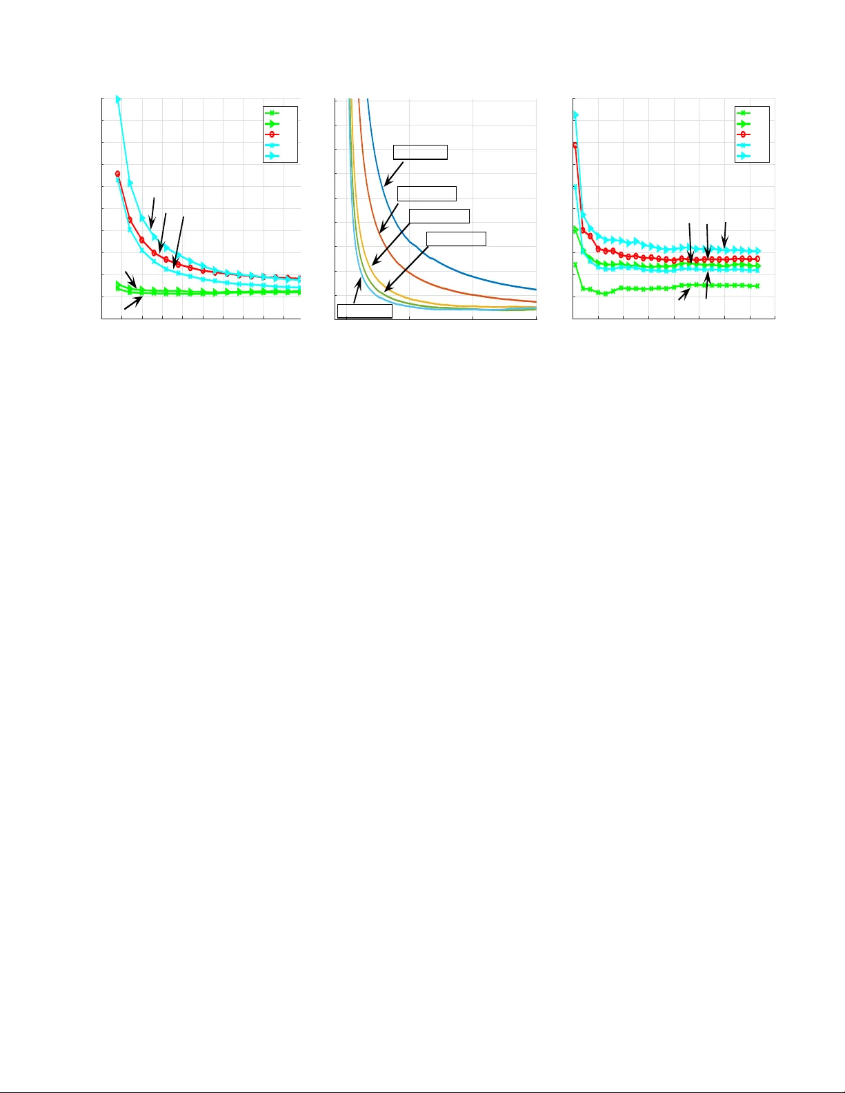
1 Online T raining of LSTM Networks in Distrib uted Systems for V ariable Length Data Sequences T olga Ergen and Suleyman S. K ozat Senior Member , IEEE Abstract —In this brief paper , we in vestigate online training of Long Short T erm Memory (LSTM) architectur es in a dis- tributed network of nodes, where each node employs an LSTM based structure f or online regr ession. In particular , each node sequentially recei ves a variable length data sequence with its label and can only exchange information with its neighbors to train the LSTM architecture. W e first provide a generic LSTM based r egression structure for each node. In order to train this structure, we put the LSTM equations in a nonlinear state space f orm f or each node and then intr oduce a highly effective and efficient Distributed Particle Filtering (DPF) based training algorithm. W e also introduce a Distributed Extended Kalman Filtering (DEKF) based training algorithm for comparison. Here, our DPF based training algorithm guarantees con vergence to the performance of the optimal LSTM coefficients in the mean squar e error (MSE) sense under certain conditions. W e achieve this performance with communication and computational complexity in the order of the first order gradient based methods. Through both simulated and real life examples, we illustrate significant performance impro vements with r espect to the state of the art methods. Index T erms —Distributed learning, online learning, particle filtering, extended Kalman filtering, LSTM networks. I . I N T R O D U C T I O N Neural networks provide enhanced performance for a wide range of engineering applications, e.g., prediction [1] and human behavior modeling [2], thanks to their highly strong nonlinear modeling capabilities. Among neural networks, es- pecially recurrent neural networks (RNNs) are used to model time series and temporal data due to their inherent memory storing the past information [3]. Howe ver , since simple RNNs lack control structures, the norm of gradient may grow or decay in a fast manner during training, i.e., the exploding and vanishing gradient issues [4]. Due to these problems, simple RNNs are insufficient to capture long and short term dependencies [4]. T o circumvent this issue, a novel RNN architecture with control structures, i.e., the Long Short T erm Memory (LSTM) network, is introduced [5]. Ho wev er , since LSTM networks ha ve additional nonlinear control structures with se veral parameters, they may also suf fer from training issues [5]. T o this end, in this brief paper , we consider online training of the parameters of an LSTM structure in a distributed network of nodes. Here, we ha ve a netw ork of nodes, where each node has a set of neighboring nodes and can only exchange information with these neighbors. In particular , each node sequentially recei ves a v ariable length data sequence This work is supported in part by TUBIT AK Contract No 115E917. The authors are with the Department of Electrical and Electron- ics Engineering, Bilkent Uni versity , Bilkent, Ankara 06800, T urkey , T el: +90 (312) 290-2336, Fax: +90 (312) 290-1223, (contact e-mail: { ergen, kozat } @ee.bilkent.edu.tr). with its label and trains the parameters of the LSTM network. Each node can also communicate with its neighbors to share information in order to enhance the training performance since the goal is to train one set of LSTM coefficients using all the av ailable data. As an example application, suppose that we hav e a database of labelled tweets and our aim is to train an emotion recognition engine based on an LSTM structure, where the training is performed in an online and distributed manner using se veral processing units. W ords in each tweet are represented by word2v ec vectors [6] and tweets are distributed to several processing units in an online manner . The LSTM architectures are usually trained in a batch setting in the literature, where all data instances are present and processed together [3]. Ho we ver , for applications in v olving big data, storage issues may arise due to keeping all the data in one place [7]. Additionally , in certain framew orks, all data instances are not av ailable beforehand since instances are re- ceiv ed in a sequential manner , which precludes batch training [7]. Hence, we consider online training, where we sequentially receiv e the data to train the LSTM architecture without storing the pre vious data instances. Note that ev en though we work in an online setting, we may still suf fer from computational power and storage issues due to large amount of data [8]. As an example, in tweet emotion recognition applications, the systems are usually trained using an enormous amount of data to achieve suf ficient performance, especially for agglutinativ e languages [6]. For such tasks distributed architectures are used. In this basic distrib uted architectures, commonly named as centralized approach [8], the whole data is distributed to dif ferent nodes and trained parameters are merged later at a central node [3]. Howe ver , this centralized approach requires high storage capacity and computational power at the central node [8]. Additionally , centralized strategies have a potential risk of failure at the central node. T o circumvent these issues, we distrib ute both the processing as well as the data to all the nodes and allo w communication only between neighboring nodes, hence, we remove the need for a central node. In particular , each node sequentially receiv es a variable length data sequence with its label and exchanges information only with its neighboring nodes to train the common LSTM parameters. For online training of the LSTM architecture in a distributed manner , one can emplo y one of the first order gradient based algorithms at each node due to their efficienc y [3] and exchange estimates among neighboring nodes as in [9]. How- ev er , since these training methods only exploit the first order gradient information, they suf fer from poor performance and con ver gence issues. As an example, the Stochastic Gradient Descent (SGD) based algorithms usually have slower con v er- gence compared to the second order methods [3], [9]. On the 2 other hand, the second order gradient based methods require much higher computational comple xity and communication load while providing superior performance compared to the first order methods [3]. Follo wing the distributed implementa- tion of the first order methods, one can implement the second order training methods in a distributed manner , where we share not only the estimates but also the Jacobian matrix, e.g., the Distributed Extended Kalman Filtering (DEKF) algorithm [10], [11]. Howe ver , as in the first order case, these sharing and combining the information at each node is adhoc, which does not provide the optimal training performance [10]. In this brief paper, to pro vide impro ved performance with respect to the second order methods while preserving both communica- tion and computational complexity similar to the first order methods, we introduce a highly ef fecti ve distributed online training method based on the particle filtering algorithm [12]. W e first propose an LSTM based model for variable length data regression. W e then put this model in a nonlinear state space form to train the model in an online and optimal manner . Our main contributions include: 1) W e introduce distrib uted LSTM training methods in an online setting for variable length data sequences. Our Distributed Particle Filtering (DPF) based training algorithm guarantees conv ergence to the optimal cen- tralized training performance in the mean square error (MSE) sense; 2) W e achieve this performance with a computational complexity and a communication load in the order of the first order gradient based methods; 3) Through simulations in volving real life and financial data, we illustrate significant performance improv ements with respect to the state of the art methods [13], [14]. The organization of this brief paper is as follows. In Section II, we first describe the v ariable length data re gression problem in a network of nodes and then introduce an LSTM based structure. Then, in Section III, we first put this structure in a nonlinear state space form and then introduce our training algorithms. In Section IV, we illustrate the merits of our algorithms through simulations. W e then finalize the brief paper with concluding remarks in Section V. I I . M O D E L A N D P RO B L E M D E S C R I P T I O N Here 1 , we consider a network of K nodes. In this network, we declare two nodes that can e xchange information as neighbors and denote the neighborhood of each node k as N k that also includes the node k , i.e., k ∈ N k . At each node k , we sequentially receiv e { d k,t } t ≥ 1 , d k,t ∈ R and matrices, { X k,t } t ≥ 1 , defined as X k,t = [ x (1) k,t x (2) k,t . . . x ( m t ) k,t ] , where x ( l ) k,t ∈ R p , ∀ l ∈ { 1 , 2 , . . . , m t } and m t ∈ Z + is the number of columns in X k,t , which can change with respect to t . In our network, each node k aims to learn a certain relation between the desired v alue d k,t and matrix X k,t . After observing X k,t and d k,t , each node k first updates its belief about the relation and then exchanges an updated information with its neighbors. After receiving X k,t +1 , each node k estimates the next signal d k,t +1 as ˆ d k,t +1 . Based on d k,t +1 , each node k suffers the 1 All column vectors (or matrices) are denoted by boldface lower (or uppercase) case letters. For a matrix A (or a vector a ), A T ( a T ) is its ordinary transpose. The time index is gi ven as subscript, e.g., u t is the vector at time t . Here, 1 (or 0 ) is a vector of all ones (or zeros) and I is the identity matrix, where the sizes of these notations are understood from the context. LS TM LS TM LS TM ...                 Mean P ool i ng                                    Mean P ool i ng                                          Fig. 1: Detailed schematic of each node k in our network. loss l ( d k,t +1 , ˆ d k,t +1 ) at time instance t + 1 . This frame work models a wide range of applications in the machine learning and signal processing literatures, e.g., sentiment analysis [6]. As an example, in tweet emotion recognition application [6], each X k,t corresponds to a tweet, i.e., the t th tweet at the node (processing unit) k . For the t th tweet at the node k , one can construct X k,t by finding word2v ec representation of each word, i.e., x ( l ) k,t for the l th word. After recei ving d k,t , i.e., the desired emotion label for the t th tweet at the node k , each node k first updates its belief about the relation between the tweet and its emotion label, and then exchanges information, e.g., the trained system parameters, with its neighboring units to estimate the next label. In this brief paper, each node k generates an estimate ˆ d k,t using the LSTM architecture. Although there exist different variants of LSTM, we use the most widely used v ariant [5], i.e., the LSTM architecture without peephole connections. The input X k,t is first fed to the LSTM architecture as illustrated in Fig. 1, where the internal equations are gi ven as [5]: i ( l ) k,t = σ ( W ( i ) k x ( l ) k,t + R ( i ) k y ( l − 1) k,t + b ( i ) k ) (1) f ( l ) k,t = σ ( W ( f ) k x ( l ) k,t + R ( f ) k y ( l − 1) k,t + b ( f ) k ) (2) c ( l ) k,t = i ( l ) k,t  g ( W ( z ) k x ( l ) k,t + R ( z ) k y ( l − 1) k,t + b ( z ) k ) + f ( l ) k,t  c ( l − 1) k,t (3) o ( l ) k,t = σ ( W ( o ) k x ( l ) k,t + R ( o ) k y ( l − 1) k,t + b ( o ) k ) (4) y ( l ) k,t = o ( l ) k,t  h ( c ( l ) k,t ) , (5) where x ( l ) k,t ∈ R p is the input vector , y ( l ) k,t ∈ R n is the output vector and c ( l ) k,t ∈ R n is the state vector for the l th LSTM unit. Moreov er , o ( l ) k,t , f ( l ) k,t and i ( l ) k,t represent the output, forget and input gates, respectively . g ( · ) and h ( · ) are set to the hyperbolic tangent function and apply vectors pointwise. Likewise, σ ( · ) is the pointwise sigmoid function. The operation  represents the elementwise multiplication of two vectors of the same size. As the coefficient matrices and the weight vectors of the LSTM architecture, we ha ve W ( . ) k , R ( . ) k and b ( . ) k , where the sizes are chosen according to the input and output vectors. Gi ven the outputs of LSTM for each column of X k,t as seen in Fig. 1, we generate the estimate for each node k as follo ws ˆ d k,t = w T k,t ¯ y k,t , (6) where w k,t ∈ R n is a vector of the regression coefficients and ¯ y k,t ∈ R n is a vector obtained by taking av erage of the LSTM outputs for each column of X k,t , i.e., known as the mean pooling method, as described in Fig. 1. 3 Remark 1: In (6), we use the mean pooling method to generate ¯ y k,t . One can also use the other pooling methods by changing the calculation of ¯ y k,t and then generate the estimate as in (6). As an example, for the max and last pooling methods, we use ¯ y k,t = max i y ( i ) k,t and ¯ y k,t = y ( m t ) k,t , respectively . All our deriv ations hold for these pooling methods and the other LSTM architectures. W e provide the required updates for different LSTM architectures in the next section. I I I . O N L I N E D I S T R I B U T E D T R A I N I N G A L G O R I T H M S In this section, we first gi ve the LSTM equations for each node in a nonlinear state space form. Based on this form, we then introduce our distrib uted algorithms to train the LSTM parameters in an online manner . Considering our model in Fig. 1 and the LSTM equations in (1), (2), (3), (4) and (5), we have the following nonlinear state space form for each node k ¯ c k,t = Ω( ¯ c k,t − 1 , X k,t , ¯ y k,t − 1 ) (7) ¯ y k,t = Θ( ¯ c k,t , X k,t , ¯ y k,t − 1 ) (8) θ k,t = θ k,t − 1 (9) d k,t = w T k,t ¯ y k,t + ε k,t , (10) where Ω( · ) and Θ( · ) represent the nonlinear mappings per- formed by the consecutive LSTM units and the mean pooling operation as illustrated in Fig. 1, and θ k,t ∈ R n θ is a param- eter vector consisting of { w k , W ( z ) k , R ( z ) k , b ( z ) k , W ( i ) k , R ( i ) k , b ( i ) k , W ( f ) k , R ( f ) k , b ( f ) k , W ( o ) k , R ( o ) k , b ( o ) k } , where n θ = 4 n ( n + p ) + 5 n . Since the LSTM parameters are the states of the network to be estimated, we also include the static equation (9) as our state. Furthermore, ε k,t represents the error in observ ations and it is a zero mean Gaussian random variable with v ariance R k,t . Remark 2: W e can also apply the introduced algorithms to different implementations of the LSTM architecture [5]. For this purpose, we modify the function Ω( · ) and Θ( · ) in (7) and (8) according to the chosen LSTM architecture. W e also alter θ k,t in (9) by adding or removing certain parameters according to the chosen LSTM architecture. A. Online T raining Using the DEKF Algorithm In this subsection, we first derive our training method based on the EKF algorithm, where each node trains its LSTM parameters without any communication with its neighbors. W e then introduce our training method based on the DEKF algorithm in order to train the LSTM architecture when we allow communication between the neighbors. The EKF algorithm is based on the assumption that the state distribution given the observations is Gaussian [11]. T o meet this assumption, we introduce Gaussian noise to (7), (8) and (9). By this, we ha ve the follo wing model for each node k   ¯ c k,t ¯ y k,t θ k,t   =   Ω( ¯ c k,t − 1 , X k,t , ¯ y k,t − 1 ) Θ( ¯ c k,t , X k,t , ¯ y k,t − 1 ) θ k,t − 1   +   e k,t  k,t υ k,t   (11) d k,t = w T k,t ¯ y k,t + ε k,t , (12) where [ e T k,t ,  T k,t , υ T k,t ] T is zero mean Gaussian process with cov ariance Q k,t . Here, each node k is able to observe only d k,t to estimate ¯ c k,t , ¯ y k,t and θ k,t . Hence, we group ¯ c k,t , ¯ y k,t and θ k,t together into a vector as the hidden states to be estimated. 1) Online T raining with the EKF Algorithm:: In this sub- section, we derive the online training method based on the EKF algorithm when we do not allow communication between the neighbors. Since the system in (11) and (12) is already in a nonlinear state space form, we can directly apply the EKF algorithm [11] as follows T ime Update: ¯ c k,t | t − 1 = Ω( ¯ c k,t − 1 | t − 1 , X k,t , ¯ y k,t − 1 | t − 1 ) (13) ¯ y k,t | t − 1 = Θ( ¯ c t | t − 1 , X k,t , ¯ y k,t − 1 | t − 1 ) (14) θ k,t | t − 1 = θ k,t − 1 | t − 1 (15) Σ k,t | t − 1 = F k,t − 1 Σ k,t − 1 | t − 1 F T k,t − 1 + Q k,t − 1 (16) Measurement Update: R = H T k,t Σ k,t | t − 1 H k,t + R k,t   ¯ c k,t | t ¯ y k,t | t θ k,t | t   =   ¯ c k,t | t − 1 ¯ y k,t | t − 1 θ k,t | t − 1   + Σ k,t | t − 1 H k,t R − 1 ( d k,t − ˆ d k,t ) Σ k,t | t = Σ k,t | t − 1 − Σ k,t | t − 1 H k,t R − 1 H T k,t Σ k,t | t − 1 , where Σ ∈ R (2 n + n θ ) × (2 n + n θ ) is the error covariance matrix, Q k,t ∈ R (2 n + n θ ) × (2 n + n θ ) is the state noise co variance and R k,t ∈ R is the measurement noise variance. Additionally , we assume that R k,t and Q k,t are known terms. W e compute H k,t and F k,t as follows H T k,t = h ∂ ˆ d k,t ∂ ¯ c ∂ ˆ d k,t ∂ ¯ y ∂ ˆ d k,t ∂ θ i    ¯ c = ¯ c k,t | t − 1 ¯ y = ¯ y k,t | t − 1 θ = θ k,t | t − 1 (17) and F k,t =     ∂ Ω( ¯ c , X k,t , ¯ y ) ∂ ¯ c ∂ Ω( ¯ c , X k,t , ¯ y ) ∂ ¯ y ∂ Ω( ¯ c , X k,t , ¯ y ) ∂ θ ∂ Θ( ¯ c , X k,t , ¯ y ) ∂ ¯ c ∂ Θ( ¯ c , X k,t , ¯ y ) ∂ ¯ y ∂ Θ( ¯ c , X k,t , ¯ y ) ∂ θ 0 0 I          ¯ c = ¯ c k,t | t ¯ y = ¯ y k,t | t θ = θ k,t | t , (18) where F k,t ∈ R (2 n + n θ ) × (2 n + n θ ) and H k,t ∈ R (2 n + n θ ) . 2) Online T raining with the DEKF Algorithm:: In this subsection, we introduce our online training method based on the DEKF algorithm for the network described by (11) and (12). In our network of K nodes, we denote the number of neighbors for the node k as η k , i.e., also called as the degree of the node k [10]. W ith this structure, the time update equations in (13), (14), (15) and (16) still hold for each node k . Howe v er , since we ha ve information exchange between the neighbors, the measurement update equations of each node k adopt the iterativ e scheme [10] as the following. For the node k at time t : φ k,t ← − [ ¯ c T k,t | t − 1 ¯ y T k,t | t − 1 θ T k,t | t − 1 ] T Φ k,t ← − Σ k,t | t − 1 For each l ∈ N k repeat: R ← − H T l,t Φ k,t H l,t + R l,t φ k,t ← − φ k,t + Φ k,t H l,t R − 1 ( d l,t − w T k,t | t − 1 ¯ y k,t | t − 1 ) Φ k,t ← − Φ k,t − Φ k,t H l,t R − 1 H T l,t Φ k,t . Now , we update the state and co variance matrix estimate as Σ k,t | t = Φ k,t [ ¯ c T k,t | t ¯ y T k,t | t θ T k,t | t ] T = X l ∈N k c ( k , l ) φ l,t , 4 where c ( k, l ) is the weight between the node k and l and we compute these weights using the Metropolis rule as follo ws c ( k , l ) =        1 / max( η k , η l ) if l ∈ N k /k 1 − P l ∈N k /k c ( k , l ) if k = l 0 if l / ∈ N k . (19) W ith these steps, we can update all the nodes in our network as illustrated in Algorithm 1. According to the procedure in Algorithm 1, the computa- tional complexity of our training method results in O ( η k ( n 8 + n 4 p 4 )) computations at each node k due to matrix and vector multiplications on lines 8 and 19 as shown in T able I. Algorithm 1 T raining based on the DEKF Algorithm 1: According to (17), compute H k,t , ∀ k ∈ { 1 , 2 , . . . , K } 2: for k = 1 : K do 3: φ k,t ← − [ ¯ c T k,t | t − 1 ¯ y T k,t | t − 1 θ T k,t | t − 1 ] T 4: Φ k,t ← − Σ k,t | t − 1 5: for l ∈ N k do 6: R ← − H T l,t Φ k,t H l,t + R l,t 7: φ k,t ← − φ k,t + Φ k,t H l,t R − 1 ( d l,t − w T k,t | t − 1 ¯ y k,t | t − 1 ) 8: Φ k,t ← − Φ k,t − Φ k,t H l,t R − 1 H T l,t Φ k,t 9: end for 10: end for 11: for k = 1 : K do 12: Using (19), calculate c ( k, l ) , ∀ l ∈ N k 13: [ ¯ c T k,t | t ¯ y T k,t | t θ T k,t | t ] T ← − P l ∈N k c ( k, l ) φ l,t 14: Σ k,t | t ← − Φ k,t 15: According to (18), compute F k,t 16: ¯ c k,t +1 | t ← − Ω( ¯ c k,t | t , X k,t , ¯ y k,t | t ) 17: ¯ y k,t +1 | t ← − Θ( ¯ c k,t +1 | t , X k,t , ¯ y k,t | t ) 18: θ k,t +1 | t ← − θ k,t | t 19: Σ k,t +1 | t ← − F k,t Σ k,t | t F T k,t + Q k,t 20: end for B. Online T raining Using the DPF Algorithm In this subsection, we first derive our training method based on the PF algorithm when we do not allow communication between the nodes. W e then introduce our online training method based on the DPF algorithm when the nodes share information with their neighbors. The PF algorithm only requires the independence of the noise samples in (11) and (12). Thus, we modify our system in (11) and (12) for the node k as follo ws a k,t = ϕ ( a k,t − 1 , X k,t ) + γ k,t (20) d k,t = w T k,t ¯ y k,t + ε k,t , (21) where γ k,t and ε k,t are independent state and measurement noise samples, respecti vely , ϕ ( · , · ) is the nonlinear mapping in (11) and a k,t , [ ¯ c T k,t ¯ y T k,t θ T k,t ] T . 1) Online T r aining with the PF Algorithm: : F or the system in (20) and (21), our aim is to obtain E [ a k,t | d k, 1: t ] , i.e., the optimal estimate for the hidden state in the MSE sense. T o achiev e this, we first obtain posterior distribution of the states, i.e., p ( a k,t | d k, 1: t ) . Based on the posterior density function, we then calculate the conditional mean estimate. In order to obtain the posterior distribution, we apply the PF algorithm [15]. In this algorithm, we hav e the samples and the correspond- ing weights of p ( a k,t | d k, 1: t ) , i.e., denoted as { a i k,t , ω i k,t } N i =1 . Based on the samples, we obtain the posterior distribution as T ABLE I: Comparison of the computational complexities of the introduced training algorithms for each node k . In this table, we also calculate the computational complexity of the SGD based algorithm by deriving exact gradient equations, howe ver , we omit these calculations due to page limit. Algorithm Computational Complexity SGD O ( n 4 + n 2 p 2 ) DEKF O ( η k ( n 8 + n 4 p 4 )) DPF O ( N ( k )( n 2 + np )) follows p ( a k,t | d k, 1: t ) ≈ N X i =1 ω i k,t δ ( a k,t − a i k,t ) . (22) Sampling from the desired distribution p ( a k,t | d k, 1: t ) is in- tractable in general so that we obtain the samples from q ( a k,t | d k, 1: t ) , which is called as importance function [15]. T o calculate the weights in (22), we use the follo wing formula w i k,t ∝ p ( a i k,t | d k, 1: t ) q ( a i k,t | d k, 1: t ) , where N X i =1 ω i k,t = 1 . (23) W e can factorize (23) such that we obtain the following recursiv e formula [15] ω i k,t ∝ p ( d k,t | a i k,t ) p ( a i k,t | a i k,t − 1 ) q ( a i k,t | a i k,t − 1 , d k,t ) ω i k,t − 1 . (24) In (24), we choose the importance function so that the v ariance of the weights is minimized. By this, we obtain particles that hav e nonnegligible weights and significantly contribute to (22) [15]. In this sense, since p ( a i k,t | a i k,t − 1 ) provides a small variance for the weights [15], we choose it as our importance function. With this choice, we alter (24) as follo ws ω i k,t ∝ p ( d k,t | a i k,t ) ω i k,t − 1 . (25) By (22) and (25), we obtain the state estimate as follo ws E [ a k,t | d k, 1: t ] = Z a k,t p ( a k,t | d k, 1: t ) d a k,t ≈ Z a k,t N X i =1 ω i k,t δ ( a k,t − a i k,t ) d a k,t = N X i =1 ω i k,t a i k,t . Although we choose the importance function to reduce the variance of the weights, the variance ine vitably increases ov er time [15]. Hence, we apply the resampling algorithm introduced in [15] such that we eliminate the particles with small weights and prevent the variance from increasing. 2) Online T r aining with the DPF Algorithm:: In this sub- section, we introduce our online training method based on the DPF algorithm when the nodes share information with their neighbors. W e employ the Markov Chain Distrib uted P article Filter (MCDPF) algorithm [12] to train our distributed system. In the MCDPF algorithm, particles mov e around the network according to the network topology . In ev ery step, each particle can randomly move to another node in the neighborhood of its current node. While randomly moving, the weight of each particle is updated using p ( d k,t | a k,t ) at the node k , hence, particles use the observations at dif ferent nodes. Suppose we consider our network as a graph G = ( V , E ) , where the v ertices V represent the nodes in our network and the edges E represent the connections between the nodes. In addition to this, we denote the number of visits to each node k in s steps by each particle i as M i ( k , s ) . Here, each particle moves to one of its neighboring nodes with a certain probability , where the mov ement probabilities of each node to 5 the other nodes are represented by the adjacency matrix, i.e., denoted as A . In this frame work, at each visit to each node k , each particle multiplies its weight with p ( d k,t | a k,t ) 2 | E ( G ) | sη k in a run of s steps [12], where | E ( G ) | is the number of edges in G and η k is the degree of the node k . From (25), we ha ve the following update for each particle i at the node k after s steps w i k,t = w i k,t − 1 K Y j =1 p ( d j,t | a i k,t ) 2 | E ( G ) | sη j M i ( j,s ) . (26) W e then calculate the posterior distribution at the node k as p ( a k,t | O k,t ) ≈ N X i =1 w i k,t δ ( a k,t − a i k,t ) , (27) where O k,t represents the observations seen by the particles at the node k until t and w i k,t is obtained from (26). After we obtain (27), we calculate our estimate for a k,t as follows E [ a k,t | O k,t ] = Z a k,t p ( a k,t | O k,t ) d a k,t ≈ Z a k,t N X i =1 ω i k,t δ ( a k,t − a i k,t ) d a k,t = N X i =1 ω i k,t a i k,t . (28) W e can obtain the estimate for each node using the same procedure as illustrated in Algorithm 2. In Algorithm 2, N ( j ) represents the number of particles at the node j and I i → j represents the indices of the particles that mov e from the node i to the node j . Thus, we obtain a distributed training algorithm that guarantees con ver gence to the optimal centralized parameter estimation as illustrated in Theorem 1. Theorem 1: F or each node k , let a k,t be the bounded state vector with a measur ement density function that satisfies the following inequality 0 < p 0 ≤ p ( d k,t | a k,t ) ≤ || p || ∞ < ∞ , (29) wher e p 0 is a constant and || p || ∞ = sup d k,t p ( d k,t | a k,t ) . Then, we have the following conver gence results in the MSE sense N X i =1 ω i k,t a i k,t → E [ a k,t |{ d j, 1: t } K j =1 ] as N → ∞ and k → ∞ . Pr oof of Theor em 1. Using (29), from [12], we obtain E  E [ π ( a t ) |{ d j, 1: t } K j =1 ] − N X i =1 ω i k,t π ( a i k,t )  2  ≤ || π || 2 ∞  C t p U ( s, υ ) + r ς t N  2 , (30) where π is a bounded function, υ is the second largest eigen- value modulus of A , ς t and C t are time dependent constants and U ( s, υ ) is a function of s as described in [12] such that U ( s, υ ) goes to zero as s goes to infinity . Since the state vector a k,t is bounded, we can choose π ( a k,t ) = a k,t . W ith this choice, ev aluating (30) as N and s go to infinity yields the results. This concludes our proof.  According to the update procedure illustrated in Algorithm 2, the computational complexity of our training method results in O ( N ( k )( n 2 + np )) computations at each node k due to matrix vector multiplications in (20) and (21) as sho wn in T able I. Algorithm 2 T raining based on the DPF Algorithm 1: Sample { a i j,t } N ( j ) i =1 from p ( a t |{ a i j,t − 1 } N ( j ) i =1 ) , ∀ j 2: Set { w i j,t } N ( j ) i =1 = 1 , ∀ j 3: for s steps do 4: Move the particles according to A 5: for j = 1 : K do 6: { a i j,t } N ( j ) i =1 ← S l ∈N j { a i l,t } i ∈I l → j 7: { w i j,t } N ( j ) i =1 ← S l ∈N j { w i l,t } i ∈I l → j 8: { w i j,t } N ( j ) i =1 ← { w i j,t } N ( j ) i =1 p ( d j,t |{ a i j,t } N ( j ) i =1 ) 2 | E ( G ) | sη j 9: end for 10: end for 11: for j=1:K do 12: Resample { a i j,t , w i j,t } N ( j ) i =1 13: Compute the estimate for node j using (28) 14: end for I V . S I M U L AT I O N S W e ev aluate the performance of the introduced algorithms on different benchmark real datasets. W e first consider the prediction performance on Hong Kong exchange rate dataset [16]. W e then e valuate the regression performance on emo- tion labelled sentence dataset [17]. For these experiments, to observe the effects of communication among nodes, we also consider the EKF and PF based algorithms without communication over a network of multiple nodes, where each node trains LSTM based on only its observations. Throughout this section, we denote the EKF and PF based algorithms without communication o ver a netw ork of multiple nodes as “EKF” and “PF”, respecti vely . W e also consider the SGD based algorithm without communication ov er a network of multiple nodes as a benchmark algorithm and denote it by “SGD”. W e first consider the Hong Kong exchange rate dataset [16]. For this dataset, we have the amount of Hong K ong dollars that can buy one United States dollar on certain days. Our aim is to estimate future exchange rate by using the values in the pre vious two days. In online applications, one can demand a small steady state error or fast conv ergence rate based on the requirements of application [18]. In this experiment, we ev aluate the con ver gence rates of the algorithms. For this purpose, we select the parameters such that the algorithms con ver ge to the same steady state error le vel. In this setup, we choose the parameters for each node k as follo ws. Since X k,t ∈ R 2 is our input, we set the output dimension as n = 2 . In addition to this, we consider a network of four nodes. F or the PF based algorithms, we choose N ( k ) = 80 as the number of particles. Additionally , we select γ k,t and ε k,t as zero mean Gaussian random v ariables with Co v[ γ k,t ] = 0 . 0004 I and V ar[ ε k,t ] = 0 . 01 , respecti vely . For the DPF based algorithm, we choose s = 3 and A = [0 1 2 0 1 2 ; 1 2 0 1 2 0; 0 1 2 0 1 2 ; 1 2 0 1 2 0] . For the EKF based algorithms, we select Σ k, 0 | 0 = 0 . 0004 I , Q k,t = 0 . 0004 I and R k,t = 0 . 01 . Moreover , according to (19), the weights between nodes are calculated as 1 / 3 . For the SGD based algorithm, we set the learning rate as µ = 0 . 1 . In Fig. 2a, we illustrate the prediction performance of the algorithms. Due to the highly nonlinear structure of our model, the EKF and DEKF based algorithms hav e slower con v ergence compared to the other algorithms. Moreover , due to only exploiting the first order gradient information, the SGD based 6 0 50 100 150 200 250 300 350 400 450 5 00 Data Length 0 0.01 0.02 0.03 0.04 0.05 0.06 0.07 0.08 0.09 0.1 Cumulative Error Financial Prediction Performance DPF PF SGD DEKF EKF DPF PF DEKF SGD EKF (a) 0 500 1000 150 0 Data Length 1 2 3 4 5 6 7 8 9 Cumulative Error × 10 -3 Comparison for the DPF Algorithm N=160,s=3,T=38.36 N=20,s=1,T=2.80 N=160,s=4,T=47.20 N=80,s=2,T=14.72 N=80,s=3,T=19.34 (b) 0 1000 2000 3000 4000 5000 6000 7000 8000 Data Length 0.08 0.09 0.1 0.11 0.12 0.13 0.14 0.15 0.16 0.17 0.18 Cumulative Error Label Prediction Performance DPF PF SGD DEKF EKF DPF DEKF PF SGD EKF (c) Fig. 2: Error performances (a) ov er the Hong K ong exchange rate dataset, (b) for different N and s combinations of the DPF based algorithm and (c) over the sentence dataset. In (b), we also provide computation times of the combinations (in seconds), i.e., denoted as T , where a computer with i5-6400 processor, 2.7 GHz CPU and 16 GB RAM is used. algorithm has also slo wer conv ergence compared to the PF based algorithms. Unlike the SGD and EKF based methods, the PF based algorithms perform parameter estimation through a high performance gradient free density estimation technique, hence, they con ver ge much faster to the final MSE lev el. Among the PF based methods, due to its distributed structure the DPF based algorithm has the fastest con ver gence rate. In order to demonstrate the ef fects of the number of particles N and the number of Markov steps s , we perform another experiment using the Hong Kong exchange rate dataset. In this experiment, we use the same setting with the previous case except Cov[ γ k,t ] = 0 . 0001 I , Σ k, 0 | 0 = 0 . 0001 I and Q k,t = 0 . 0001 I . In Fig. 2b, we observe that as s and N increase, the DPF based algorithm obtains a faster con ver gence rate and a lower final MSE v alue. Ho we ver , as s and N increase, the marginal performance improv ement becomes smaller with respect to the pre vious s and N values. Furthermore, the computation time of the algorithm increases with increasing s and N values. Thus, after a certain selection, a further increase does not worth the additional computational load. Therefore, we use N ( k ) = 80 and s = 3 in our pre vious simulation. Other than the Hong Kong exchange rate dataset, we consider the emotion labelled sentence dataset [17]. In this dataset, we have the v ector representation of each w ord in an emotion labelled sentence. In this e xperiment, we ev aluate the steady state error performance of the algorithms. Thus, we choose the parameters such that the con ver gence rate of the algorithms are similar . T o provide this setup, we select the parameters for each node k as follo ws. Since the number of words varies from sentence to sentence in this case, we hav e a variable length input regressor , i.e., defined as X k,t ∈ R 2 × m t , where m t represents the number of words in a sentence. For the other parameters, we use the same setting with the Hong K ong exchange rate dataset except N ( k ) = 50 , Cov[ γ k,t ] = (0 . 025) 2 I , Σ k, 0 | 0 = (0 . 025) 2 I , Q k,t = (0 . 025) 2 I and µ = 0 . 055 . In Fig. 2c, we illustrate the label prediction performance of the algorithms. Again due to the highly nonlinear structure of our model, the EKF based algorithm has the highest steady state error v alue. Additionally , the SGD based algorithm also has a high final MSE value compared to the other algorithms. Furthermore, the DEKF based algorithm achieves a lower final MSE value than the PF based method thanks to its distributed structure. Ho wev er , since the DPF based method utilizes a powerful gradient free density estimation method while ef fectiv ely sharing information between the neighboring nodes, it achie ves a much smaller steady state error value. V . C O N C L U D I N G R E M A R K S W e studied online training of the LSTM architecture in a distributed network of nodes for regression and introduced online distrib uted training algorithms for v ariable length data sequences. W e first proposed a generic LSTM based model for variable length data inputs. In order to train this model, we put the model equations in a nonlinear state space form. Based on this form, we introduced distributed extended Kalman and particle filtering based online training algorithms. In this way , we obtain effecti ve training algorithms for our LSTM based model. Here, our distributed particle filtering algorithm guarantees con ver gence to the optimal centralized parameter estimation in the MSE sense under certain conditions. W e achiev e this performance with communication and computa- tional complexity in the order of the first order methods [3]. Through simulations inv olving real life and financial data, we illustrate significant performance improvements with respect to the state of the art methods [13], [14]. R E F E R E N C E S [1] D. F . Specht, “ A general regression neural network, ” IEEE T ransactions on Neural Networks , vol. 2, no. 6, pp. 568–576, Nov 1991. [2] Y . Meng, Y . Jin, and J. Y in, “Modeling activity-dependent plasticity in bcm spiking neural networks with application to human behavior recognition, ” IEEE T ransactions on Neural Networks , vol. 22, no. 12, pp. 1952–1966, Dec 2011. [3] A. C. Tsoi, “Gradient based learning methods, ” in Adaptive pr ocessing of sequences and data structures . Springer , 1998, pp. 27–62. [4] Y . Bengio, P . Simard, and P . Frasconi, “Learning long-term dependen- cies with gradient descent is dif ficult, ” IEEE T ransactions on Neural Networks , vol. 5, no. 2, pp. 157–166, Mar 1994. [5] S. Hochreiter and J. Schmidhuber, “Long short-term memory , ” Neural Comput. , vol. 9, no. 8, pp. 1735–1780, Nov . 1997. 7 [6] S. V osoughi, P . V ijayaraghav an, and D. Ro y , “T weet2vec: Learning tweet embeddings using character-lev el CNN-LSTM encoder-decoder , ” CoRR , vol. abs/1607.07514, 2016. [7] D. Wilson and T . R. Martinez, “The general inef ficiency of batch training for gradient descent learning, ” Neural Networks , v ol. 16, no. 10, pp. 1429 – 1451, 2003. [8] X. W u et al. , “Data mining with big data, ” IEEE T ransactions on Knowledge and Data Engineering , vol. 26, no. 1, pp. 97–107, Jan 2014. [9] K. Y uan et al. , “On the conver gence of decentralized gradient descent, ” SIAM Journal on Optimization , vol. 26, no. 3, pp. 1835–1854, 2016. [10] F . S. Cattiv elli and A. H. Sayed, “Diffusion strategies for distributed kalman filtering and smoothing, ” IEEE Tr ansactions on Automatic Contr ol , vol. 55, no. 9, pp. 2069–2084, Sept 2010. [11] B. D. Anderson et al. , Optimal filtering . Courier Corporation, 2012. [12] S. H. Lee and M. W est, “Conv ergence of the markov chain distributed particle filter (MCDPF), ” IEEE Tr ansactions on Signal Processing , vol. 61, no. 4, pp. 801–812, Feb 2013. [13] J. A. P ´ erez-Ortiz et al. , “Kalman filters improve LSTM network per - formance in problems unsolv able by traditional recurrent nets, ” Neural Networks , vol. 16, no. 2, pp. 241–250, 2003. [14] A. W . Smith and D. Zipser , “Learning sequential structure with the real-time recurrent learning algorithm, ” International Journal of Neural Systems , vol. 1, no. 02, pp. 125–131, 1989. [15] P . M. Djuric et al. , “Particle filtering, ” IEEE Signal Processing Maga- zine , vol. 20, no. 5, pp. 19–38, 2003. [16] E. W . Frees, “Regression modelling with actuarial and financial applications. ” [Online]. A v ailable: http://instruction.b us.wisc.edu/jfrees/ jfreesbooks/Regression%20Modeling/BookW ebDec2010/data.html [17] M. Lichman, “UCI machine learning repository , ” 2013. [18] A. H. Sayed, Fundamentals of adaptive filtering . John W iley & Sons, 2003.