Delta-Ramp Encoder for Amplitude Sampling and its Interpretation as Time Encoding

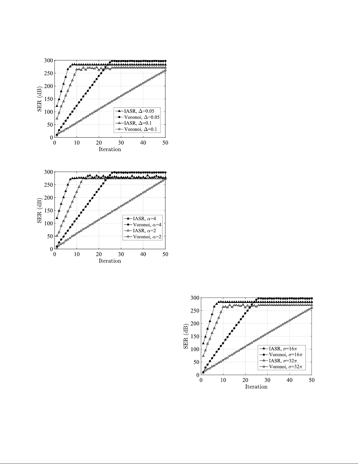
IEEE TRANSA CTIONS ON SIGNAL PR OCESSING 1 Delta-Ramp Encoder for Amplitude Sampling and its Interpretation as T ime Encoding Pablo Mart ´ ınez-Nue vo, Member , IEEE, Hsin-Y u Lai, Student Member , IEEE, and Alan V . Oppenheim, Life F ellow , IEEE Abstract —The theoretical basis f or con ventional acquisition of bandlimited signals typically relies on unif orm time sampling and assumes infinite-precision amplitude values. In this paper , we explore signal repr esentation and recovery based on uniform amplitude sampling with assumed infinite precision timing in- formation. The approach is based on the delta-ramp encoder which consists of applying a one-level lev el-crossing detector to the result of adding an appropriate sawtooth-like wavef orm to the input signal. The output samples are the time instants of these level crossings, thus repr esenting a time-encoded version of the input signal. For theoretical purposes, this system can be equivalently analyzed by re versibly transforming through ramp addition a nonmonotonic input signal into a monotonic one which is then uniformly sampled in amplitude. The monotonic function is then represented by the times at which the signal crosses a predefined and equally-spaced set of amplitude values. W e refer to this technique as amplitude sampling. The time sequence generated can be interpreted alternativ ely as nonunif orm time sampling of the original source signal. W e derive duality and frequency-domain properties for the functions involv ed in the transformation. Iterative algorithms are proposed and imple- mented for recov ery of the original source signal. As indicated in the simulations, the pr oposed iterative amplitude-sampling algorithm achiev es a faster conver gence rate than frame-based reconstruction for nonuniform sampling. The performance can also be improved by appropriate choice of the parameters while maintaining the same sampling density . Index T erms —Sampling theory , level-cr ossing sampling, nonuniform sampling and reconstruction, iterative algorithms. I . I N T R O D U C T I O N T HE theoretical foundation of con ventional time sampling typically relies on the sampling theorem for bandlimited signals [1]–[3], which states that bandlimited signals can be perfectly represented by infinite-precision amplitude values taken at equally-spaced time instants appropriately separated. c  2019 IEEE. Personal use of this material is permitted. Permission from IEEE must be obtained for all other uses, in any current or future media, including reprinting/republishing this material for advertising or promotional purposes, creating ne w collecti ve works, for resale or redistribution to servers or lists, or reuse of any copyrighted component of this work in other works. This work was supported in part by T exas Instruments Leadership Uni- versity Program. The work of P . Mart ´ ınez-Nuev o was also supported in part by Fundaci ´ on Rafael del Pino, Madrid, Spain. The work of H. Lai was also supported in part by the Jacobs Fellowship and the Siebel Fellowship. P . Mart ´ ınez-Nuev o was with the Department of Electrical Engineering and Computer Science, Massachusetts Institute of T echnology . He is now with the research department at Bang & Olufsen, 7600 Struer, Denmark (e-mail: pmnuev o@alum.mit.edu). H. Lai and A. V . Oppenheim are with the Department of Electrical Engineering and Computer Science, Massachusetts Institute of T echnology , Cambridge MA 02139 USA (e-mail: hsinyul@mit.edu; av o@mit.edu). Digital Object Identifier 10.1109/TSP .2019.2904027 In this paper, we propose a signal representation based on equally-spaced amplitude samples with infinite-precision tim- ing information. W e introduce the delta-ramp encoder that generates a time encoded version of the input signal and show how this sampling and reconstruction process can be theoret- ically analyzed based on the amplitude sampling concept also introduced in this paper . Signal representation based on discrete amplitudes and continuous time has pre viously been studied and utilized in a number of contexts. In [4] signal representation consists of the real and complex zeros of a bandlimited signal. Logan’ s theorem [5] characterizes a subclass of bandpass signals that can be completely represented, up to a scaling factor , by their zero crossings. Practical algorithms for recovery from zero crossings of periodic signals in this class hav e been proposed in [6]. Arbitrary bandlimited signals can also be implicitly described by the zero crossings of a function resulting from an in vertible transformation [7]–[9]—for e xample, the addition of a sinew ave [10, Theorem 1]. In principle, interpolation is possible through Hadamard’ s factorization [11, Chapter 5] although there are more ef ficient techniques in terms of con vergence rate [12]–[15]. Zero-crossings ha ve also been studied in relation to wavelet transforms [16]. In this case, stable reconstruction can be achiev ed by including additional information about the original signal. The extension from zero crossings to multiple levels, in the context of data compression, was in vestigated in [17]. In that work, a sample is generated whenever the source signal crosses a predefined set of threshold levels. The time instants of the crossings and the le vel-crossings directions were utilized to represent the signal although time was still quantized due to practical considerations. A practical continuous-time version of level-crossing sampling was later proposed in [18]. Asynchronous delta modulation [19] is, also, in some sense, a precursor of level-crossing sampling since it generates a positiv e or negativ e pulse at time instants when the change in signal amplitude surpasses a fixed quantity . In the context of asynchronous sigma-delta modulation systems, In the context of asynchronous sigma-delta modulation sys- tems, the connection between time-based representation and local averages of bandlimited signals was shown in [20] where frame-based reconstruction can be carried out [21, Theorem 7]. This sampling process can then be vie wed as a representation of a signal as a stream of pulses where processing can be performed directly in the pulse domain [22]. In this paper , we study the time encoding process of the IEEE TRANSA CTIONS ON SIGNAL PROCESSING 2 delta-ramp encoder (see Fig. 1) and reconstruction from the generated time sequence. W e show that this system can be analyzed theoretically based on the more general concept of amplitude sampling with the signal represented by the time sequence of equally-spaced level crossings of a monotonic transformation of the input signal as would be generated, for example, by an amplitude quantizer with equal step sizes. In principle, if a signal were monotonic, then the crossings of equally-spaced amplitude lev els would generate an ordered time sequence { t n } which could be considered as a rep- resentation of the signal. Under appropriate conditions, this corresponds to uniform sampling in amplitude with the signal information contained in the time sequence { t n } . Nonmono- tonic signals can be reversibly transformed into monotonic ones which are then uniformly sampled in amplitude. W e refer to this technique as amplitude sampling. As discussed in Section II where we introduce the delta- ramp encoder , when the reversible transformation consists of adding a ramp with appropriate slope, a practical implemen- tation to generate the identical ordered time sequence { t n } is the delta-ramp encoder shown in Fig. 1. The time sequence generated by the delta-ramp encoder and that obtained by uniform amplitude sampling after ramp addition are identical. For the theoretical analysis of the delta-ramp encoder in this paper , we utilize the interpretation of the time sequence { t n } as deriv ed from uniform amplitude sampling of the monotonic function obtained by ramp addition. Section III defines the general concept of amplitude sampling. In sections IV, V, and VI we deriv e duality as well as time- and frequency-domain properties relating the functions present in the transformation. The structure of these functions suggest an iterative recon- struction algorithm for numerical recovery of the source signal from the amplitude samples. This algorithm is discussed in Section VII with simulations and comparisons with frame- based reconstruction from nonuniform time samples. Throughout the paper , we refer to ˆ f as the Fourier transform of the function f gi ven by ˆ f ( ξ ) = Z R f ( t ) e − i 2 π ξt d t, ξ ∈ R . (1) The Fourier inv ersion formula then takes the following form f ( t ) = Z R ˆ f ( ξ ) e + i 2 π ξt d ξ , t ∈ R . (2) Note that the units for ξ can be interpreted to be Hz. W e say that a function f is of moderate decrease or moderate decay if it is continuous and there exists A > 0 such that | f ( t ) | ≤ A/ (1 + t 2 ) for all t ∈ R . I I . D E LT A - R A M P E N C O D E R The delta-ramp encoder is represented by the block diagram depicted in Fig. 1. The lev el detector produces an impulse at times at which the input signal reaches the value ∆ . For ease of illustration, assume the ramp-segment generator initiates a ramp with slope α > 0 that abruptly shifts down by ∆ in amplitude whenev er an impulse arriv es. Assume α is chosen such that ˜ g ( t ) is monotonic in each interv al between successi ve impulses. Fig. 1. Equiv alent representation of the amplitude sampling process. Fig. 2 shows an example of the signals in volved in the process. By construction, the ramp segments of the function r ( t ) present the same slope. This manifests itself in the presence of an continuous ramp of slope α separated by multiples of ∆ for each corresponding segment. Consequently , the function ˜ g ( t ) satisfies the following ˜ g ( t ) = f ( t ) + αt − k ∆ (3) for t ∈ ( t k , t k +1 ] and k ∈ Z . Thus, ˜ g ( t k +1 ) = ∆ = f ( t k +1 ) + αt k +1 − k ∆ (4) which giv es ( k + 1)∆ = g ( t k +1 ) for all k ∈ Z where g ( t ) = α t + f ( t ) . Consider now the time instants { t n } that satisfy g ( t n ) = n ∆ = αt n + f ( t n ) . As a result of the one-to-one correspondence between amplitude values and time instants due to the monotonicity of g ( t ) , it follows that { t k } = { t n } . Thus, the delta encoder generates impulses at the same time instants at which g ( t ) crosses the set of amplitude lev els { n ∆ } . In summary , the delta-ramp encoder produces a represen- tation of the input signal as a sequence of time instants, or time codes. This time encoding mechanism can be alterna- tiv ely viewed as lev el-crossing sampling of the function g ( t ) or nonuniform sampling of f ( t ) , i.e. f ( t n ) = n ∆ − αt n . Moreov er , the function g ( t ) , assuming appropriate regularity conditions, has an inv erse function t ( g ) which is effecti vely sampled uniformly in the amplitude domain with samples corresponding to these time instants. Therefore, the sampling process of the delta-ramp encoder can be interpreted as uni- formly sampling the function t ( g ) . In principle, it is possible to generalize this concept by considering any transformation that generates a monotonic function g ( t ) . W e formalize this concept in the next section. I I I . P R I N C I P L E O F A M P L I T U D E S A M P L I N G Amplitude sampling and reconstruction as dev eloped in this paper is then based on the principle of reversibly representing and then sampling a time function g ( t ) in the form t ( g ) and then sampling in g . This requires that g ( t ) be monotonic which means that if the source signal is nonmonotonic, it must first be re versibly transformed into a strictly monotonic function through a transformation φ . As illustrated in Fig. 3, the resulting function φ ( f ( t )) is then uniformly sampled. The time instants { t n } at which φ ( f ( t )) crosses the predefined set of amplitude values { n ∆ } implicitly represent the source signal, i.e. φ ( f ( t n )) = n ∆ where ∆ > 0 is the separation between IEEE TRANSA CTIONS ON SIGNAL PROCESSING 3 Fig. 2. Illustration of the different wav eforms inv olved in the system shown in Fig. 1. consecutiv e levels. Each of the time instants is paired exactly with one amplitude le vel. Thus, there exists a one-to-one correspondence between amplitude values and time instants. The sequence of time instants together with knowledge of ∆ is sufficient information to describe the sampling process. Thus, it can be interpreted as a form of time encoding. Amplitude sampling corresponds to signal-dependent nonuniform time sampling with the sampling density depen- dent on the source signal and the choice of the transformation φ . Fig. 3. Principle of amplitude sampling based on a transformation φ of the source signal f resulting in a monotonic function φ ( f ( t )) . W e have shown in Section II that, when a ramp of appro- priate slope is used, amplitude sampling is equi valent to the samples generated by a delta-ramp encoder . In fact, it can be shown that many delta-modulation systems can be interpreted as amplitude sampling. For a detailed analysis of the latter , the interested reader is referred to [23, Chapter 4]. I V . T R A N S F O R M AT I O N B Y R A M P A D D I T I O N There exist a myriad of transformations φ that can poten- tially generate a monotonic function from a giv en f . Among the simplest is the addition of a ramp with a sufficiently large slope. Suppose the original signal f is continuous, and it is possible to construct the strictly monotonic function g ( t ) = αt + f ( t ) for some α ∈ R . Then, the sampling process consists of the sequence of time instants { t n } satisfying g ( t n ) = αt n + f ( t n ) = n ∆ for some ∆ > 0 . As indicated earlier , for analysis purposes in this paper, it is con venient to interpret the time sequence { t n } as resulting from sampling uniformly in amplitude the monotonic function u = g ( t ) = αt + f ( t ) . In the context of this transformation, there exists an in verse function g − 1 ( u ) that we choose to express in the form g − 1 ( u ) = u/α + h ( u ) for some amplitude- time function h . This interpretation suggests that this trans- formation can also be vie wed as a mapping from f to the associated function h . A. Mapping between f and h The addition of a ramp represents a mapping, parametrized by the slope of the ramp, between the original signal and the function h . W e denote this mapping by M α , i.e. M α f = h which can be vie wed as the addition of the ramp to obtain the monotonic function g and, after inv erting g , subtracting the ramp u/α to obtain h . The re verse procedure to recov er f from h consists of adding a ramp of slope u/α to h and utilizing the inv ertibility of g − 1 as well as the correspondence between g and f . This in verse mapping is denoted by M α − 1 and satisfies M α − 1 h = f . Fig. 4 illustrates the one-to-one correspondence between f and h . These mappings are also summarized in equation form as [24] f ( t ) = − αh ( f ( t ) + α t ) , h ( u ) = − 1 α f ( h ( u ) + u α ) . (5) Fig. 4. Illustration of the in vertibility of the transformation between f and h when g ( t ) = αt + f ( t ) and g − 1 ( u ) = u/α + h ( u ) . As is evident from Fig. 4 and (5) there is a duality between M α and its in verse. It is possible to interpret (5) as a signal- dependent warping operation that obtains f from h and vice versa. The addition of a ramp in amplitude sampling also generates an underlying mapping, dependent on f or h , between time t and amplitude u . Both mappings can be easily seen from (5) in its matrix form and the corresponding inv erse matrix:  f ( t ) t  =  − α 0 1 1 /α   h ( u ) u  , (6) IEEE TRANSA CTIONS ON SIGNAL PROCESSING 4  h ( u ) u  =  − 1 /α 0 1 α   f ( t ) t  . (7) The duality implies that any properties of h inherited by assumptions made on f hold for f if the same assumptions are instead imposed on h . B. The Sampling Pr ocess Amplitude sampling produces a sequence of time instants corresponding to n ∆ = g ( t n ) = αt n + f ( t n ) where ∆ > 0 . This sampling process results then in g − 1 and h being uni- formly sampled in amplitude, i.e. g − 1 ( n ∆) = n ∆ /α + h ( n ∆) (8) and h ( n ∆) = t n − n ∆ /α. (9) C. Sampling Density As noted earlier , amplitude sampling in the form presented here can be vie wed as equi valent to nonuniform time sampling. In this setting, stable reconstruction algorithms typically im- pose conditions on the sequence of sampling instants as for example the Landau rate [25] for bandlimited signals. In order to gain insight into the time-sampling density inherent in our amplitude-sampling process, assume the source signal f has a bounded deri vati ve, i.e. | f 0 ( t ) | ≤ B for some B > 0 and that | α | > B so that the function g ( t ) = αt + f ( t ) is strictly monotonic. Then the time between successi ve samples satisfies the inequality ∆ | α | + B ≤ | t n +1 − t n | ≤ ∆ | α | − B . (10) where ∆ > 0 is the separation between consecutiv e amplitude lev els. The bounds in (10) are consistent with intuition. For exam- ple, assume that α is positiv e. The deriv ative of g is bounded by α + B which provides the minimum attainable time separa- tion between crossings. Similarly , the maximum separation is essentially limited by α − B . The quantization step ∆ repre- sents the change in amplitude necessary to produce a sample. Additionally , when α achiev es sufficiently large values, the bounds for time separation become closer , or equiv alently , the time sequence becomes more uniform. W e can observe this effect in (10) where amplitude is approximately a scaled version of the time axis. D. Iterative Algorithm for the Realization of M α In this section, we propose an iterativ e algorithm for the implementation of M α to generate h ( u ) from f ( t ) . By duality , an equi valent algorithm can be used for the implemention of M α − 1 to generate f ( t ) from h ( u ) . For ease of illustration, we consider a modified version of the transformation M α by considering ˜ h ( u ) = − αh ( αu ) . This transformation, which we denote by ˜ M α , is then giv en by: f ( t ) = ˜ h ( 1 α f ( t ) + t ) , ˜ h ( u ) = f ( − 1 α ˜ h ( u ) + u ) . (11) Equations (11) form the basis for the iterativ e algorithm formalized in the following theorem. Theor em 1: Let the function f be Lipschitz continuous with constant < α and suppose that sup t ∈ R | f ( t ) | ≤ A . Then, the function values ˜ h ( u ) = ( ˜ M α f )( u ) for u ∈ R can be obtained by the iteration ˜ h n +1 ( u ) = f ( u − 1 α ˜ h n ( u )) (12) for n ≥ 0 where ˜ h 0 ( u ) = f ( u ) and ˜ h n ( u ) → ˜ h ( u ) as n → ∞ . The detailed proof is carried out in Appendix A. Fig. 5. Illustration of the iteration described in Theorem 1 with the initialization t 0 = u 0 . As used in the preceding, the v alue of ˜ h ( u 0 ) can be obtained from the first equality in (11). In particular, ˜ h ( u 0 ) = f ( t ∗ ) where t ∗ is the v alue that satisfies u 0 = t ∗ + f ( t ∗ ) /α . The solution is unique since the slope of the ramp, in absolute value, is alw ays greater than the maximum v alue of the deriv ativ e of f . As sho wn in Fig. 5, t 0 is the time instant at which the ramp αt 0 − αt intersects the function f ( t ) . In the same way , the value of the ( n + 1) -th iteration can be viewed as the solution of αt − ( αu 0 − f ( t n )) = 0 . In other words, we iterativ ely construct a straight line passing through the point ( u 0 , f ( t n )) . The intersection with the horizontal axis then corresponds to the v alue of t n +1 . Note that the process for recov ering h from f is analogous to the one presented in Theorem 1, i.e. the iteration takes the form f n +1 ( t ) = ˜ h ( f n ( t ) /α + t ) . V . S P E C T R A L P R O P E RT I E S Assumptions made on the source signal f are naturally reflected in the structure of h . In this section, we assume that f is a bandlimited function and derive properties regarding the spectral content of the amplitude-time function h . The duality between f and h = M α f implies that similar conclusions can be made about f when h is assumed to be bandlimited. In exploring the spectral content of h we assume that f is bandlimited to σ rad/s with σ > 0 and bounded in amplitude, i.e. | f ( t ) | < A for some A . W e further assume that the decay of f ( t ) for t real satisfies | f ( t ) | ≤ A/ (1 + t 2 ) . In principle, the extension to square-integrable functions is straightforward. W ith our assumptions on f , Bernstein’ s inequality [26] pro- vides the bound | f 0 ( t ) | ≤ Aσ for all t ∈ R . This bound gurantees that the function u defined as u = g ( t ) = αt + f ( t ) . (13) IEEE TRANSA CTIONS ON SIGNAL PROCESSING 5 will be strictly monotonic whenev er | α | > Aσ . The function h is then giv en by h ( u ) = g − 1 ( u ) − u/α . From Theorem 2 below it follo ws that the decay of the Fourier transform of h , denoted by ˆ h ( ξ ) , satisfies ˆ h ( ξ ) = O ( e − 2 π | ξ | b ) as ξ → ∞ where b > 0 is determined by the dif ference | α | − Aσ . Theor em 2: Let f ( t ) : R → R be a continuous function bandlimited to σ > 0 rad/s. Assume further that | f ( t ) | ≤ A/ (1 + t 2 ) for all t ∈ R and some A > 0 . Construct the function u = g ( t ) = αt + f ( t ) (14) for | α | > Aσ . Then, there exists g − 1 ( u ) for all u ∈ R and a constant C > 0 such that the Fourier transform of h ( u ) = g − 1 ( t ) − u/α satisfies | ˆ h ( ξ ) | ≤ C e − 2 π | ξ | b for any 0 ≤ b < a such that a = | α | σ log  | α | Aσ  − | α | − Aσ σ . (15) and ξ ∈ R . The detailed proof is carried out in Appendix B. As anticipated, the rate of decay of the F ourier transform at infinity depends on | α | − Aσ . The difference is logarithmic in the first term and linear in the second one. The larger the difference the faster the decay at infinity . Note that a > 0 always holds since | α | > Aσ . Assuming α > 0 , this difference is precisely impacting the highest slope portions in h , or, equiv alently , the regions in which f 0 is smallest. The underlying reason being that the deriv ati ve of g − 1 is the reciprocal of g , i.e. ( g − 1 ( u )) 0 = 1 /g 0 ( g − 1 ( u )) for all u ∈ R . Informally , it is the tilted regions in the shape of h are responsible, to some extent, for the high-frequency content. It should be emphasized that any bandlimited function will naturally be in the class of signals whose spectrum exhibits at least exponential decay at infinity . Howe ver , Theorem 3 stated below asserts that f and h cannot be simultaneously bandlimited. The precise statement in the description of the theorem guarantees this property with the possible exception of, at most, one v alue of α . For practical purposes, we can ignore this isolated case. Theor em 3: Under the conditions of Theorem 2 and unless f is constant, the function h is nonbandlimited for e very α > Aσ with at most one exception. The detailed proof is carried out in Appendix C. In the singular case, in which f is a constant, it can be shown through the constructiv e process of M α by ramp addition that h is constant as well, specifically , for f = A , then h = − A/α . From another point of view , according to (5), the function f results, in general, from h with a nonlinear warping of the independent v ariable. When either of the two functions is constant, the warping is affine. Therefore, in this case, the bandlimited property is preserved [27]. In our context the conclusion follows directly from (5) that if either f or h is constant, the other must be also. More generally , if | α | increases significantly , the warping function becomes approximately linear since f ( t ) is negligible compared to αt , i.e. f ( t ) ≈ − αh ( αt ) . This is consistent with (15) where an increase of | α | produces a f aster decay at infinity of ˆ h . V I . T I M E - D O M A I N D E C AY P RO P E RT I E S In some sense, h inherits characteristics of f since it is a ”time-warped” version of f . In this section, we show the connections between the properties of f and h in the time domain with the relationship between f and h as specified in (5) which explicitly requires that the slope of the ramp added to f and the slope of the ramp subtracted to obtain h be exact in verses. Intuitiv ely , it is not surprising that the function h should present decay properties similar to those of f once the unbounded growth of the ramp component has been subtracted. In particular, when the slopes of the two ramps are reciprocals of each other , the decay of h will match that of f . Otherwise h does not decay appropriately on the real line (see Proposition 3 in Appendix D). The transformation M α also has an impact on the L p norms of the respectiv e functions with the parameter α playing a crucial role. It can be shown—refer to Proposition 4 in Appendix D—that the decay on the real line of both functions is related by || h || p = 1 α 1 − 1 p || f || p , p ∈ [1 , ∞ ] . (16) Not only does h belong to L p ( R ) if f does, but their respectiv e norms are also related by a scaling factor which is precisely α . Indeed, for very large values of | α | , the ramp approaches the vertical axis, thus reducing the range of h and decreasing the norm. In terms of a sense of distance, consider h 1 = M α f 1 and h 2 = M α f 2 . The transformation M α preserves the L 1 distance (see Proposition 5 in Appendix D), i.e. || h 1 − h 2 || 1 = || f 1 − f 2 || 1 . (17) By duality , these properties hold irrespecti ve of the role of each function as an input or output. V I I . R E C O N S T R U C T I O N F RO M D E LT A - R A M P E N C O D I N G The time encoding performed by the delta-ramp encoder can be seen, under the amplitude sampling perspective, as signal- dependent nonuniform time sampling of the source signal f based on uniform time sampling of the associated amplitude- time function h . If f is bandlimited, then as was shown in Section V h is not bandlimited and consequently cannot be exactly reconstructed through bandlimited interpolation. Our reconstruction approach begins by initially using sinc interpolation as an approximation. This is then extended to an iterativ e algorithm that achie ves accurate recovery . Throughout this entire section, we assume that the source signal f is bandlimited to σ rad/s, and | f ( t ) | ≤ A/ (1 + t 2 ) for A > 0 and all t ∈ R . A. Bandlimited Interpolation Algorithm (BIA) The approximate reconstruction of f based on sinc interpo- lation of h is depicted in Fig. 6. From this approximation to h an approximation to f is generated through M α − 1 which is then lowpass filtered since f is assumed to be bandlimited. In particular , the D/C system is defined by the relationship h ∆ ( u ) = X n ∈ Z h ( n ∆)sinc( u/ ∆ − n ) . (18) IEEE TRANSA CTIONS ON SIGNAL PROCESSING 6 Note that the samples of h are related to { t n } as h ( n ∆) = t n − n ∆ /α , n ∈ Z . The moti vation to perform bandlimited interpolation from the samples of h is based on the exponential decay of its spectrum. Since h is nonbandlimited, the alias- ing error can be characterized by the following bound (see Proposition 6 in Appendix E) || h − h ∆ || ∞ ≤ C 0 a e − π b ∆ (19) for any 0 ≤ b < a and some C 0 > 0 where a is giv en in (15). Then, the error in (19) is then controlled both by the difference | α | − Aσ and the quantization step size ∆ . As already discussed, increasing the difference | α | − Aσ produces, in some sense, a function h with a faster high-frequency spectral decay and therefore one that is more approximately bandlimited. Since the quantization step size ∆ also deter- mines the sampling density of h , by decreasing ∆ the aliasing error of the bandlimited interpolation is also reduced. By an appropriate combination of a sufficiently large α and/or a sufficiently small ∆ , the function h ∆ ( u ) + u/α can be assumed to be in vertible. W e then obtain f ∆ = M 1 /α h ∆ . The function f ∆ is nonbandlimited since h ∆ is bandlimited (see Theorem 3). Thus, we obtain the bandlimited interpolation ˜ f by passing f ∆ through a lowpass filter with cutof f frequency σ rad/s. Fig. 6. Approximate reconstruction procedure for a bandlimited source signal f such that h = M α f . The block D/C is a discrete-to-continuous operation in volving sinc interpolation with period ∆ . B. Iterative Amplitude Sampling Reconstruction (IASR) The bandlimited interpolation algorithm (BIA) forms the basis for an iterative algorithm which we refer to as the Iterativ e Amplitude Sampling Reconstruction (IASR) algo- rithm as detailed in Algorithm 1 and illustrated in Fig. 7. The time instants { t n } represent both samples of f and the associated function h . Similarly to BIA, the sample values { h ( n ∆) = t n − n ∆ /α } are the input to the algorithm assuming we also know the parameters α and ∆ in volv ed in the sampling process. Note that if the initialization satisfies h 0 ≡ 0 and f 0 ≡ 0 , the first iteration corresponds precisely to BIA, i.e. f 1 ( t ) = ˜ e 1 ( t ) = ˜ f ( t ) for all t ∈ R . Thus, the emphasis is placed on the reconstruction of h from its uniform amplitude samples and then the bandlimited constraint is imposed on the successiv e approximations to f with the objecti ve of iterativ ely reducing the error || ˜ e k ( t ) || 2 . C. Simulation Results In all of the simulations in this section, the source signal f is chosen as white noise bandlimited to σ rad/s and bounded by A > 0 . The quantization step size ∆ and the parameter Fig. 7. Block diagram representation of the iterativ e amplitude sampling reconstruction (IASR) algorithm. Algorithm 1 IASR algorithm 1: Input: { t n } , α , ∆ , and σ 2: { h ( n ∆) } ← { t n − n ∆ /α } 3: Initialize h 0 and f 0 4: do 5: { η n } ← { h ( n ∆) − h k ( n ∆) } 6: η ∆ ( u ) ← P n ∈ Z η n sinc( u/ ∆ − n ) 7: e ∆ ← M 1 /α η ∆ 8: ˜ e k ← LPF σ ( e ∆ )  LPF σ ( · ) represents a lowpass filtering operation with cutoff frequency σ rad/s. 9: f k +1 ← f k + ˜ e k 10: h k +1 ← M α f k +1 11: while 0 ≤ k < K or || ˜ e k || 2 >   K and  are parameters establishing the stopping criteria. 12: return f k α are chosen so that the sampling density is greater than or equal to the Landau rate [25], which, in our case, is given by π /σ . W e choose as a measure of approximation error the signal-to-error ratio (SER) giv en by SER = 10 log 10  || f || 2 2 || f − f k || 2 2  (20) where f k is the k -th iteration. Since amplitude sampling also implies nonuniform time sampling on the source signal f , we also directly apply a nonuniform reconstruction algorithm to recover f in order to illustrate the particular factors influencing the performance of IASR. Specifically , we compare IASR to the V oronoi method dev eloped in [21, Theorem 8.13] that presents the best tradeoff between conv ergence rate and approximation error among the frame-based methods described therein. W e chose the V oronoi method since it has been sho wn to present a con vergence rate approximately the same as reconstruction from local av erages which has been used in other time encoding techniques for bandlimited signals [20]. Based on the bounds in (10) for the time instants, it is straightforward to see that the sampling instants in an amplitude sampling setting satisfy the require- ments of the V oronoi method for an appropriate choice of the parameters. In particular, it can be shown that it is sufficient that ∆ | α | − Aσ > π σ . (21) IEEE TRANSA CTIONS ON SIGNAL PROCESSING 7 In initializing both algorithms, the 0 -th iteration in both IASR and the V oronoi method is assumed to be zero. (a) (b) Fig. 8. Performance comparison between IASR, A WM, and BIA, for a broadband input signal bandlimited and bounded; (a) ∆ is changed while α is fixed; (b) α is changed while ∆ is fixed. In Fig. 8, we hav e modified separately the parameters α and ∆ . In reducing the value of the quantization step size ∆ , the transformed function αt + f ( t ) will clearly cross more amplitude levels per unit of time. Similarly , when the slope of the ramp added to f is increased in absolute value, it also causes an increase in the lev el-crossing density . Thus, both ef fects result in an increase of the sampling density , and as shown in the figure, the rate of conv ergence improv es. Howe ver , it can be observed that the rate of con vergence is faster in the IASR case. The first iteration in IASR achiev es a better approximation than the V oronoi method although the rate of conv ergence appears to be highly insensitiv e to this change of parameters. On the other hand, the V oronoi method is significantly impacted by the change in sampling density . Moreov er , it requires sev eral iterations until it obtains the same approximation performance as the first iteration in IASR. As shown in Fig. 9 the same conclusions hold if we increase the ov ersampling ratio by considering signals with smaller bandwidths and, at the same time, keeping α and ∆ fixed. Thus far , we have focused on modifying the sampling density . Additionally , due to the structure of the sampling process in amplitude sampling, it is also possible to keep the sampling density fixed while changing both α and ∆ accordingly . The rate of con ver gence in the V oronoi method is determined by the maximal separation between consecutive sampling instants. W ith constant sampling density , the per- formance of the V oronoi method does not change, as shown in Fig. 10. Ho we ver , IASR presents an improv ement in the rate of con vergence. This is not surprising since the difference | α | − Aσ has increased, which likely results in a better approximation of the sinc interpolation in IASR. When the input signal is highly ov ersampled, we have empirically observed that the V oronoi method has a faster rate of conv ergence. Nev ertheless, when the sampling instants become increasingly sparse approaching the Landau rate, IASR performs significantly better . In summary , ov erall, IASR appears to hav e better per- formance than the V oronoi method in terms of speed of con vergence when the sampling density approaches the Lan- dau rate. Changes in the sampling density have a higher impact on the con ver gence in the V oronoi method than in IASR. Moreover , IASR performance can also be improved by increasing the difference | α | − Aσ while keeping the sampling density inv ariant. In [24], a scaling of the input signal also produces an increase in the speed of conv ergence. This performance improvement of IASR over the V oronoi method may be due to the characteristics of the sampling instants. Specifically the sampling instants in IASR inherently incorporate the amplitude sampling structure and therefore contain more information initially than more general nonuni- form sampling would. In some sense, this may suggest that IASR is designed to more effecti vely exploit the structure of this particular sampling process which implicitly is signal dependent and consequently signal information is implicitly embedded in both the sampling times and the sample values. Fig. 9. Performance comparison between IASR and the V oronoi method when the bandwidth σ is changed, and α and ∆ are fixed. D. Computational Complexity In the previous results, we have compared the performance of both algorithms in terms of con ver gence rate. Regarding IEEE TRANSA CTIONS ON SIGNAL PROCESSING 8 Fig. 10. Performance comparison between IASR and the V oronoi method when the sampling density is fixed and α and ∆ are changed. operations per iteration, the IASR algorithm consists mainly of bandlimited interpolation, a lowpass filtering operation, and the two transformations M α and M 1 /α . The bandlimited interpolation can be equiv alently seen as a lowpass filtering operation. From a theoretical perspective, both transformations M α and M 1 /α only entail the addition of a ramp where the in verse can be interpreted through a relabeling of the axes t and u = g ( t ) . Howe ver , in practice, we hav e considered in our simulations uniformly ov ersampled finite-length signals. Thus, in a practical setting, transformations of the form M α take uniform samples to nonuniform samples. Due to the over - sampling, we chose to perform linear interpolation to obtain an approximation to the corresponding uniform samples. The V oronoi method mainly consists of a zero-order hold and a lowpass filtering operation. Then, obtaining the function values at the nonuniform instants of time, i.e. f k ( t n ) , requires additional computation since they are not directly given by the first two operations. Fig. 11 shows a comparison of the reconstruction accuracy in terms of computation time for both methods. It is important to emphasize that these results depend on the software imple- mentation and the hardware platform. In this case, we used the MA TLAB en vironment. Among the se veral ways of simulating a lowpass filtering operation, we utilized the FFT and IFFT algorithms. From the simulations performed, we observe that the computation time per iteration is comparable. This suggests that the conclusions drawn above—i.e. when considering re- construction accurac y versus number of iterations—can also apply here. V I I I . C O N C L U S I O N W e presented the delta-ramp encoder , a form of time encod- ing where the time sequence generated is directly related to both uniform and nonuniform sampling of the corresponding associated signals. This sampling process can be analyzed theoretically as amplitude sampling which represents a signal with equally-spaced amplitude values and infinite-precision timing information by re versibly transforming the source sig- nal. This transformation provides the perspecti ve of viewing Fig. 11. Performance comparison between IASR and the V oronoi method based on computation time for a specific hardware and software imple- mentation. The solid markers represent the reconstruction accuracy of the corresponding iteration. amplitude sampling as uniform sampling of an associated amplitude-time function or equiv alently as nonuniform time sampling of the source signal. The properties of both func- tions are connected by a duality relationship. Similarly , an iterativ e algorithm for recovery was proposed and ev aluated that exploits the particular characteristics of the sampling instants in amplitude sampling. As opposed to more general nonuniform reconstruction algorithms, the con vergence rate can be improved while maintaining the sampling density constant. A P P E N D I X A P RO O F O F T H E O R E M 1 According to (11), obtaining ˜ h ( u 0 ) for some fixed u 0 ∈ R is equiv alent to finding some t ∗ ∈ R such that u 0 = t ∗ + f ( t ∗ ) /α since ˜ h ( u 0 ) = f ( t ∗ ) . Therefore, we have to find the roots of t = u 0 − 1 α f ( t ) , v u 0 ( t ) (22) for t ∈ R . It is easy to see that v u 0 ( t ) is Lipschitz continuous for some constant K < 1 . Furthermore, there alw ays e xists some  ≥ A/α such that v u o : I → I where I = [ u 0 − , u 0 +  ] . Thus, the Banach fixed-point theorem [28] guarantees the uniqueness and existence of a solution. Moreov er, it ensures con vergence with the follo wing bounds for the error | t n +1 − t ∗ | ≤ K | t n − t ∗ | (23) for n ≥ 0 where t 0 ∈ I and t n +1 = v u 0 ( t n ) . Then, the iteration can be equiv alently expressed in terms of the functional composition form as ˜ h n +1 ( u 0 ) = f ( u 0 − 1 α ˜ h n ( u 0 )) . (24) Since u 0 was chosen arbitrarily , the same conclusions hold for any u 0 ∈ R .  IEEE TRANSA CTIONS ON SIGNAL PROCESSING 9 A P P E N D I X B P RO O F O F T H E O R E M 2 For ease of notation, we will substitute the real variable t by x throughout the proof of the theorem (i.e. we will refer to f ( x ) instead of f ( t ) ). Then, the complex variable z ∈ C is expressed as z = x + iy for x, y ∈ R . W e will also use the complex variable w = u + iv for u, v ∈ R when appropriate. Define the open disk in the complex plane centered at z o and of radius r > 0 as D r ( z o ) = { z ∈ C : | z − z o | < r } (25) and use D r ( z o ) for its closure. Let us introduce some concepts that will be used throughout the proof. A function complex differentiable at ev ery point in a region Ω ⊆ C is said to be holomorphic in Ω . If the function is holomorphic ov er the whole complex plane, it is referred to as entire. An entire function f is of exponential type if there exists constants M , τ > 0 so that | f ( z ) | ≤ M e τ | z | for all z ∈ C . If σ = inf τ taken over all τ satisfying the latter inequality , it is said to be of exponential type σ . W e first introduce se veral results that will become useful in the proof of the theorem. Lemma 1: Let f be a holomorphic function in some region Ω ⊆ C with po wer series f ( z ) = P ∞ n =0 a n ( z − z o ) n at z o ∈ Ω . Consider a disk of radius R centered at z o such that Ω contains the disk and its closure. If a 1 6 = 0 and | a 1 | > ∞ X n =2 | a n | nR n − 1 , (26) then f is injectiv e in any open disk of radius r ≤ R . Pr oof 1: W ithout loss of generality assume z o = 0 , thus the power series expansion of f around the origin is gi ven by f ( z ) = P ∞ n =0 a n z n for all z ∈ Ω . T ake z 1 , z 2 ∈ D R (0) ⊂ Ω such that z 1 6 = z 2 and recall that for any z , w ∈ C the following identity holds ( z n − w n ) = ( z − w )( z n − 1 + z n − 2 w + . . . . . . + z w n − 2 + w n − 1 ) . (27) W e can write    f ( z 2 ) − f ( z 1 ) z 2 − z 1    =    a 1 + ∞ X n =2 a n z n 2 − z n 1 z 2 − z 1    =    a 1 + ∞ X n =2 a n ( z n − 1 2 + z n − 2 2 z 1 + . . . . . . + z 2 z n − 2 1 + z n − 1 1 )    ≥ | a 1 | − ∞ X n =2 | a n | nR n − 1 . where the last inequality follows from the rev erse triangle inequality and the fact that | z 1 | , | z 2 | ≤ R . Thus, if | a 1 | − P ∞ n =2 | a n | nR n − 1 > 0 , then f ( z 2 ) − f ( z 1 ) 6 = 0 and f ( z ) is injectiv e in D r ( z o ) for any r ≤ R .  Pr oposition 1: Let f : U → V be a bijective continuous function. Consider a set Ω such that its closure Ω is strictly contained in U , then f ( ∂ Ω) = ∂ f (Ω) . Pr oof 2: Consider x ∈ ∂ Ω , which is clearly a limit point of Ω . W e know there exist a con vergent sequence x n → x where x n 6 = x for n ≥ 1 and x n ∈ Ω . By continuity , f ( x n ) → f ( x ) is a con vergent sequence in V . As f is a bijection from U to V , f ( x n ) 6 = f ( x ) for all n ≥ 1 , thus f ( x ) ∈ f (Ω) . Moreover , f ( x ) 6 = f ( x 0 ) for all x 0 ∈ Ω , therefore f ( x ) ∈ ∂ f (Ω) for all x ∈ ∂ Ω . It follows that f ( ∂ Ω) ⊆ ∂ f (Ω) . Now , we claim that for e very y ∈ ∂ Ω there exists an x ∈ ∂ Ω such that y = f ( x ) . Imagine this is not true and there exists an x o ∈ U \ ∂ Ω such that y o = f ( x o ) . From our previous discussion, it is clear that x o cannot be in Ω , then imagine x o ∈ U \ Ω . Since f is continuous and bijectiv e, we can choose a suf ficiently small  > 0 such that f − 1 ( D  ( y o )) ⊂ D δ ( x o ) and D δ ( x o ) ∩ Ω = ∅ for some δ > 0 . Howe ver , as y o is a point in the boundary , it holds that D  ( y o ) ∩ f (Ω) 6 = ∅ . Thus, there exist an x 1 ∈ Ω such that f ( x 1 ) = y 0 for some y 0 ∈ D  ( y o ) . At the same time, there also exists an x 2 ∈ f − 1 ( D  ( y o )) such that f ( x 2 ) = y 0 , where x 1 6 = x 2 . This contradicts the bijectivity assumption, thus f ( ∂ Ω) ⊇ ∂ f (Ω) which together with f ( ∂ Ω) ⊆ ∂ f (Ω) gives f ( ∂ Ω) = ∂ f (Ω) .  Pr oposition 2: Suppose f ( z ) is an entire function of expo- nential type σ such that | f ( x ) | ≤ A/ (1 + x 2 ) for all x ∈ R . Then, the follo wing bound holds for all z ∈ C | f ( z ) | ≤ Ae σ | y | 1 + x 2 . (28) Pr oof 3: By assumption, | f ( z ) | ≤ Ae σ | z | for all z ∈ C . Construct the function F ( z ) = (1 / A )(1 + x 2 ) e iσ z f ( z ) , then F is bounded by 1 on the positiv e imaginary and positiv e real axis. If we consider the first quadrant Q = { z ∈ C : x > 0 , y > 0 } , it is clear that there exists constants C, c > 0 such that | F ( z ) | ≤ C e c | z | for z ∈ Q . W e conclude by the Phragm ´ en-Lindel ¨ of theorem [11, Chapter 4, Theorem 3.4] that | F ( z ) | ≤ 1 for all z in Q . This implies that | f ( z ) | ≤ Ae σ y / (1 + x 2 ) for z ∈ Q . Using the same argument, one can sho w that the same is true in the second quadrant. For the third and fourth quadrants we use instead the function F ( z ) = (1 / A )(1 + x 2 ) e − iσ z f ( z ) , which shows that (28) also holds for y ≤ 0 .  The function f is of moderate decrease and bandlimited to [ − σ , σ ] rad/s. By the Pale y-W iener theorem [11, Chapter 4, Theorem 3.3] [29, Theorem X], f is an entire function of exponential type σ . Then, using Bernstein’ s inequality [26], | f 0 ( x ) | ≤ σ A . Now , we can split the proof of the theorem in three steps. Step 1. W e claim that the function u = g ( x ) = α x + f ( x ) admits a real analytic in verse function whenever α > σ A . It is clear that g ( x ) is analytic for all x ∈ R since it is the sum of two analytic functions on the whole real line. Moreover , g ( x ) is a strictly increasing monotone function because | f 0 ( x ) | ≤ Aσ and α > Aσ , which implies g 0 ( x ) > 0 . The Real Analytic In verse Function theorem [30, Theorem 1.4.3] guarantees that for a point x o where g 0 ( x o ) 6 = 0 , there exists a neighborhood J o of x o and a real analytic function g − 1 defined on an open interval I o containing g ( x o ) satisfying ( g − 1 ◦ g )( x ) = x for x ∈ J o and ( g ◦ g − 1 )( u ) = u for y ∈ I o . Since g 0 ( x ) 6 = 0 for all real x , it is always possible for any giv en x 1 ∈ R to find an IEEE TRANSA CTIONS ON SIGNAL PROCESSING 10 x 2 / ∈ J 1 such that J 1 ∩ J 2 6 = ∅ . Thus, by analytic continuation, we conclude that g − 1 ( u ) is analytic on the whole real line. Step 2. W e show that the function g − 1 ( w ) is analytic in a region containing the horizontal strip S a = { w ∈ C : | Im( w ) | < a, where a = α σ log  α σ  − α − σ σ } . (29) The function g ( z ) = α z + f ( z ) is an entire function of exponential type σ and admits a po wer series e xpansion around x ∈ R g ( z ) = αz + ∞ X n =0 f ( n ) ( x ) n ! ( z − x ) n (30) for all z ∈ C . By Bernstein’ s inequality [26], the deriv atives of f are bounded on the real line by | f ( n ) ( x ) | ≤ Aσ n . W e now look for a region where g ( z ) is injectiv e. Using Lemma 1, g ( z ) is injecti ve in a disk of radius R > 0 whene ver | α + f 0 ( x ) | > A R ∞ X n =2 n ( σ R ) n n ! = Aσ ( e Rσ − 1) (31) or , equi valently R < 1 σ log  1 + | α + f 0 ( x ) | Aσ  . (32) The right-hand side of this e xpression is lo wer bounded by (1 /σ ) log (1 + ( α − Aσ ) / Aσ ) > 0 , since | f 0 ( x ) | ≤ Aσ < α for all x ∈ R . Thus, it is always possible to choose a disk of positiv e radius satisfying this lo wer bound such that g ( z ) is injectiv e. Let us fix an R satisfying this lower bound. Remember that holomorphic functions are open mappings, i.e. they map open sets to open sets. Thus, g ( z ) maps an open disk of radius R to the open set g ( D R ( x )) . By continuity , g ( D R ( x )) is also connected since D R ( x ) is connected. Therefore, the mapping g ( z ) : D R ( x ) → g ( D R ( x )) represents a holomorphic bijection, thus its in verse is also holomorphic. Moreov er, the in verse agrees with g − 1 ( u ) for real u ∈ g ( D R ( x )) . Thus, it represents the analytic continuation of g − 1 ( u ) on u ∈ g ( D R ( x )) . In fact, we can always choose a disk D R ( x 0 ) such that g ( D R ( x )) ∩ g ( D R ( x 0 )) 6 = ∅ , where the inv erse functions defined on their respectiv e images take the same value in the intersection for real u . Again, by analytic continuation, we can analytically extend g − 1 ( u ) to g ( D R ( x )) ∪ g ( D R ( x 0 )) . Repeating this process for all real x , we obtain the analytic continuation of g − 1 ( u ) in the open set Ω = ∪ x ∈ R g ( D R ( x )) . W e want to find an a > 0 such that S a ⊆ Ω . Using Lemma 1, the boundary of the disk ∂ D R ( x ) is mapped bijectively to ∂ g ( D R ( x )) . Therefore, the largest radius ρ for a disk centered at g ( x ) such that D ρ ( g ( x )) ⊆ g ( D R ( x )) for all x ∈ R is given by ρ = inf x ∈ R sup | z − x | = R {| g ( z ) − g ( x ) | : D | g ( z ) − g ( x ) | ( g ( x )) ⊆ g ( D R ( x )) } . (33) W e can use the power series expansion of g around x to find a lower bound for ρ in the following manner | g ( z ) − g ( x ) | = | α ( z − x ) + ∞ X n =1 a n ( z − x ) n | ≥ αR − ∞ X n =1 Aσ n n ! R n = αR − A ( e Rσ − 1) . for | z − x | = R . The right-hand side of the last expression represents a strictly concav e function of R , thus the maximum is achieved for R = 1 σ log  α Aσ  > 0 (34) which is positiv e as α > Aσ and satisfies the upper bound in (32). Setting the value of R as in (34), we can write | g ( z ) − g ( x ) | ≥ ρ ≥ α σ log  α Aσ  −  α − Aσ σ  (35) for all x ∈ R and | z − x | = R . This implies that S a ⊆ Ω for any a such that a ≤ α σ log  α Aσ  −  α − Aσ σ  . (36) Step 3. W e show that h ( w ) is of moderate decay on each horizontal line | Im( w ) | < a , uniformly in | y | < a . First, we note that since f is an entire function of exponential type σ and is of moderate decrease along the real line, by Proposition 2 | f ( z ) | ≤ Ae σ | y | 1 + x 2 (37) for all z ∈ C . Let us now fix an R satisfying (34), then we hav e a bijection from D R ( x 0 ) to g ( D R ( x 0 )) for some x 0 ∈ R . Therefore, z = g − 1 ( w ) , where w ∈ g ( D R ( x )) and z ∈ D R ( x 0 ) . Since | y | < R for z ∈ D R ( x 0 ) , we also have | f ( z ) | = | αz − g ( z ) | ≤ Ae σ R / (1 + x 2 ) , or equi v alently | w − αg − 1 ( w ) | ≤ Ae σ R 1 + ( g − 1 ( u )) 2 (38) whenev er w ∈ g ( D R ( x )) and z ∈ D R ( x 0 ) . Using the reverse triangle inequality in the previous expression for real w , we can also obtain | g − 1 ( u ) | ≥ | u | α − Ae σ R α . (39) which is true for all u ∈ R since x = g − 1 ( u ) holds for all real x and u as shown in the first step of the proof. Define the function for all real u ψ ( u ) = ( | u | /α − Ae σ R /α if | u | /α > Ae σ R /α 0 otherwise (40) which clearly satisfies | g − 1 ( u ) | ≥ | ψ ( u ) | . Make β = 1 /α and multiply both sides of (38) by 1 /α to see that | h ( w ) | = | w /α − g − 1 ( w ) | . Combining these expressions, we can then write for some A 0 > 0 and w ∈ g ( D R ( x 0 )) | h ( w ) | ≤ Ae σ R /α 1 + g − 1 ( u ) 2 ≤ Ae σ R /α 1 + ψ ( u ) 2 ≤ A 0 1 + u 2 (41) As our choice of x 0 was arbitrary , this is true for any x 0 ∈ R and | h ( u + iv ) | is of moderate decrease along horizontal lines. IEEE TRANSA CTIONS ON SIGNAL PROCESSING 11 Therefore, the function h ( w ) is analytic on the strip S a and it is of moderate decrease on each horizontal line | Im( w ) | = v , uniformly in | v | < a , as long as β = 1 /α . By [11, Chapter 4, Theorem 2.1], we conclude that there exists a constant C > 0 such that | ˆ h ( ξ ) | ≤ C e − 2 π bξ for any 0 ≤ b < a .  A P P E N D I X C P RO O F O F T H E O R E M 3 Construct the function g ( z ) = αz + f ( z ) where f is not constant. By Picard’ s little theorem [31, 16.22], there exists at most one value α > Aσ that f 0 ( z ) does not take. For the rest of them, there always exists a z o ∈ C such that g 0 ( z o ) = α + f 0 ( z o ) = 0 . Then, it is possible to write g ( z ) − a 0 = ( z − z o ) 2 [ a 2 + a 3 ( z − z o ) + a 4 ( z − z o ) 2 + . . . ] . (42) Therefore, the function g ( z ) − a o has a zero of order ≥ 2 at z o . By the Local Mapping Theorem [32, Chapter 3, Theorem 11], g is n -to-1 near z o for n ≥ 2 . Using the argument of analytic continuation of local biholomorphisms in the proof of Theorem 2, we conclude that the analytic extensions of h around g ( z o ) are multi valued. This excludes the possibility of h being entire, thus, the restriction of h to the real line cannot be bandlimited. If f ( z ) = C for some C > 0 , then h ( u ) = − C /α , which is bandlimited in the distrib utional sense.  A P P E N D I X D T I M E - D O M A I N D E C AY P R O P E RT I E S Pr oposition 3: Under the conditions of Theorem 2, construct h ( u ) = g − 1 ( u ) − β u for u ∈ R and some β ∈ R . Then, the function h is of moderate decrease if and only if β = 1 /α . Pr oof 4: The backward direction, i.e. assuming β = 1 /α , has been prov ed in Theorem 2. For the forward direction, assume on the contrary that β 6 = 1 /α . From (38), we have the following bound    | g − 1 ( u ) | − | u | /α    ≤ A/α. (43) Therefore, using the rev erse triangle inequality and the pre- vious expression, we arriv e at the follo wing for large enough u | h ( u ) | = | g − 1 ( u ) − β u | ≥    | g − 1 ( u ) | − β | u |    ≥    | u |    β − 1 α    − A α    . (44) Clearly , the right-hand side grows linearly without bound. Thus, | h ( u ) | is unbounded for β 6 = 1 /α and cannot be of moderate decrease.  Pr oposition 4: Under the conditions of Theorem 2, the following relationship holds || h || p = 1 α 1 − 1 p || f || p (45) whenev er 1 ≤ p < ∞ . Pr oof 5: Using (5) and the change of variables u = f ( t ) + αt , it is clear that for any e ven number p || h || p p = Z R h ( f ( t ) + αt ) p ( f 0 ( t ) + α )d t = 1 α p Z R f ( t ) p f 0 ( t )d t + 1 α p − 1 || f || p p . (46) W e now show that the first term on the right-hand side vanishes. First note that by the fundamental theorem of cal- culus, R R f 0 ( t )d t = 0 for any continuous function satisfying lim | t |→∞ f ( t ) = 0 . Thus, we arriv e at the following Z R f ( t ) p f 0 ( t )d t = 1 p + 1 Z R ( f ( t ) p +1 ) 0 d t = 0 (47) since f ( t ) p +1 is also of moderate decay . Therefore, || h || p = || f || p /α ( p − 1) /p . Now , for any number p ≥ 1 , we can choose a collection of intervals such that f ( t ) ≥ 0 for t ∈ ( a n , a n +1 ) and f ( t ) ≤ 0 for t ∈ ( b m , b m +1 ) for all m, n ∈ Z . Thus, we can write Z R | f ( t ) | p f 0 ( t )d t = X n ∈ Z Z a n +1 a n f ( t ) p f 0 ( t )d t − X m ∈ Z Z b m +1 b m f ( t ) p f 0 ( t )d t. (48) For each n ∈ Z , we then hav e that Z a n +1 a n f ( t ) p f 0 ( t )d t = f ( t ) p +1 p + 1    a n +1 a n = 0 (49) since f ( a n ) p +1 = 0 for all n ∈ Z . The same is true for the second term of the right-hand side of (48). Note that we allow to have intervals of the form ( c, ∞ ) or ( −∞ , d ) for any c, d ∈ R and the same holds true since lim | t |→∞ f ( t ) p +1 = 0 for p ≥ 1 . Therefore, Z R | f ( t ) | p f 0 ( t )d t = 0 (50) and || h || p = || f || p /α ( p − 1) /p for any number p ≥ 1 .  Pr oposition 5: Under the conditions of Theorem 2, the following relationship holds || h 1 − h 2 || 1 = || f 1 − f 2 || 1 (51) where h 1 = M α f 1 and h 2 = M α f 2 . Pr oof 6: Note that | h 1 ( u ) − h 2 ( u ) | = | g − 1 1 ( u ) − g − 1 2 ( u ) | and | f 1 ( t ) − f 2 ( t ) | = | g 1 ( t ) − g 2 ( t ) | , thus by Fubini’ s theorem [33, Theorem 4.1.6] we arri ve at the following || h 1 − h 2 || 1 = Z R | g − 1 1 ( u ) − g − 1 2 ( u ) | d u = Z R 2 1 Γ d t d u || f 1 − f 2 || 1 = Z R | g 1 ( t ) − g 2 ( t ) | d t = Z R 2 1 Λ d t d u where Γ = { ( t, u ) ∈ R 2 : t ∈ R , min { g 1 ( t ) , g 2 ( t ) } ≤ u ≤ max { g 1 ( t ) , g 2 ( t ) }} Λ = { ( t, u ) ∈ R 2 : u ∈ R , min { g − 1 1 ( u ) , g − 1 2 ( u ) } ≤ t ≤ max { g − 1 1 ( u ) , g − 1 2 ( u ) }} . IEEE TRANSA CTIONS ON SIGNAL PROCESSING 12 For an arbitrary ( t o , u o ) ∈ Γ , t o ≤ max { g − 1 1 ( u o ) , g − 1 2 ( u o ) } and t o ≥ min { g − 1 1 ( u o ) , g − 1 2 ( u o ) } since g 1 and g 2 are strictly increasing. This implies that Γ ⊇ Λ . Using the same reasoning, we obtain Γ ⊆ Λ which implies that Γ = Λ . Thus, the inte grals are the same.  A P P E N D I X E Pr oposition 6: If h ∆ is the bandlimited approximation to h , then there exists a C 0 > 0 such that || h − h ∆ || ∞ ≤ C 0 a e − π b ∆ (52) for any 0 ≤ b < a where a = α σ log( α Aσ ) − α − Aσ σ . Pr oof 7: Since h ( u ) is continuous and of moderate decrease, ˆ h ( ξ ) is also continuous. Moreover , we know from Theorem 2 that | ˆ h ( ξ ) | ≤ C e − b 2 π | ξ | for some C > 0 and 0 ≤ b < a where a is defined in (15). Clearly , ˆ h is Lebesgue measurable and absolutely integrable. Thus, by the generalized form of W eiss’ s theorem [34] we can bound the approximation error as | h ( u ) − h ∆ ( u ) | ≤ 2 Z | ξ | > 1 / 2∆ | ˆ h ( ξ ) | d ξ ≤ 4 C Z ξ> 1 / 2∆ e − 2 π ξb d ξ = 4 C 2 π b e − π b ∆ (53) for all u ∈ R .  R E F E R E N C E S [1] E. T . Whittaker, “XVIII.—On the functions which are represented by the expansions of the interpolation-theory , ” Proceedings of the Royal Society of Edinbur gh , vol. 35, pp. 181–194, 1915. [2] V . A. Kotelnikov , “On the carrying capacity of the ether and wire in telecommunications, ” in Material for the F irst All-Union Confer ence on Questions of Communication, Izd. Red. Upr . Svyazi RKKA, Moscow , 1933. [3] C. E. Shannon, “Communication in the presence of noise, ” Pr oceedings of the IRE , vol. 37, no. 1, pp. 10–21, 1949. [4] F . Bond and C. Cahn, “On sampling the zeros of bandwidth limited signals, ” IRE Tr ansactions on Information Theory , vol. 4, no. 3, pp. 110–113, 1958. [5] B. F . Logan, “Information in the zero crossings of bandpass signals, ” Bell System T echnical Journal , vol. 56, no. 4, pp. 487–510, 1977. [6] S. Roweis, S. Mahajan, and J. Hopfield, “Signal reconstruction from zero-crossings, ” August 1998, draft (accessed May 2016) https://www .cs.nyu.edu/ roweis/papers/log an.ps. [7] S. J. Haavik, “The conv ersion of the zeros of noise, ” Master’s thesis, Univ ersity of Rochester, Rochester, NY , 1966. [8] I. Bar-Da vid, “ An implicit sampling theorem for bounded bandlimited functions, ” Information and Control , vol. 24, no. 1, pp. 36–44, 1974. [9] R. Kumaresan and Y . W ang, “ A new real-zero conv ersion algorithm, ” in Pr oceedings 2000 IEEE International Conference on Acoustics, Speech, and Signal Processing . , vol. 1, 2000, pp. 313–316 vol.1. [10] R. J. Duf fin and A. C. Schaef fer, “Some properties of functions of exponential type, ” Bulletin of the American Mathematical Society , vol. 44, no. 4, pp. 236–240, 1938. [11] E. M. Stein and R. Shakarchi, Complex analysis , ser. Princeton Lectures in Analysis, II. Princeton Univ ersity Press, Princeton, NJ, 2003. [12] J. Selva, “Efficient sampling of band-limited signals from sine wav e crossings, ” IEEE Tr ans. Signal Processing , vol. 60, no. 1, pp. 503–508, 2012. [13] S. Kay and R. Sudhaker , “ A zero crossing-based spectrum analyzer, ” IEEE T ransactions on Acoustics, Speech and Signal Processing , vol. 34, no. 1, pp. 96–104, 1986. [14] T . V . Sreenivas and R. J. Niederjohn, “Zero-crossing based spectral analysis and svd spectral analysis for formant frequency estimation in noise, ” IEEE T ransactions on Signal Pr ocessing , vol. 40, no. 2, pp. 282– 293, 1992. [15] R. Kumaresan and N. Panchal, “Encoding bandpass signals using zero/lev el crossings: a model-based approach, ” Audio, Speech, and Language Pr ocessing, IEEE T ransactions on , vol. 18, no. 1, pp. 17– 33, 2010. [16] S. Mallat, “Zero-crossings of a wavelet transform, ” IEEE T ransactions on Information Theory , vol. 37, no. 4, pp. 1019–1033, 1991. [17] J. W . Mark and T . D. T odd, “ A nonuniform sampling approach to data compression, ” IEEE T rans. Commun. , vol. 29, no. 1, pp. 24–32, 1981. [18] Y . Tsividis, “Continuous-time digital signal processing, ” Electron. Lett. , vol. 39, no. 21, pp. 1551–1552, 2003. [19] H. Inose, T . Aoki, and K. W atanabe, “ Asynchronous delta-modulation system, ” Electr on. Lett. , vol. 2, no. 3, pp. 95–96, 1966. [20] A. A. Lazar and L. T . T ´ oth, “T ime encoding and perfect recov ery of bandlimited signals, ” in Acoustics, Speech, and Signal Pr ocessing, 2003. Pr oceedings.(ICASSP’03). 2003 IEEE International Conference on , vol. 6. IEEE, 2003, pp. VI–709. [21] H. G. Feichtinger and K. Gr ¨ ochenig, “Theory and practice of irregular sampling, ” W avelets: mathematics and applications , pp. 305–363, 1994. [22] M. McCormick, “Digital pulse processing, ” Master’ s thesis, Mas- sachusetts Institute of T echnology , September 2012. [23] P . Mart ´ ınez-Nuev o, “ Amplitude sampling for signal representation, ” Ph.D. dissertation, Massachusetts Institute of T echnology , 2016. [24] H. Lai, “Reconstruction methods for level-crossing sampling, ” Master’s Thesis, EECS, MIT , June 2016. [25] H. J. Landau, “Necessary density conditions for sampling and interpo- lation of certain entire functions, ” Acta Mathematica , vol. 117, no. 1, pp. 37–52, July 1967. [26] S. N. Bernstein, Lec ¸ ons sur les pr opri ´ et ´ es extr ´ emales et la meilleure appr oximation des fonctions analytiques d’une variable r ´ eelle . Paris, 1926. [27] S. Azizi, D. Cochran, and J. McDonald, “On the preservation of bandlimitedness under non-affine time warping, ” in Proc. Int. W orkshop on Sampling Theory and Applications , 1999. [28] S. Banach, “Sur les op ´ erations dans les ensembles abstraits et leur application aux ´ equations int ´ egrales, ” Fund. Math , vol. 3, no. 1, pp. 133–181, 1922. [29] R. E. A. C. Pale y and N. W iener , F ourier transforms in the complex domain . American Mathematical Soc., 1934, vol. 19. [30] S. G. Krantz and H. R. Parks, A primer of real analytic functions . Springer Science & Business Media, 2002. [31] W . Rudin, Real and complex analysis , 3rd ed. McGraw-Hill Education, 1986. [32] L. V . Ahlfors, Complex analysis: an introduction to the theory of analytic functions of one complex variable , 2nd ed. McGra w-Hill Book Company , 1966. [33] D. W . Stroock, Essentials of inte gration theory for analysis . Springer Science & Business Media, 2011, vol. 262. [34] J. L. Brown, Jr ., “On the error in reconstructing a non-bandlimited function by means of the bandpass sampling theorem, ” J. Math. Anal. Appl. , vol. 18, pp. 75–84, 1967.