How Entropic Regression Beats the Outliers Problem in Nonlinear System Identification

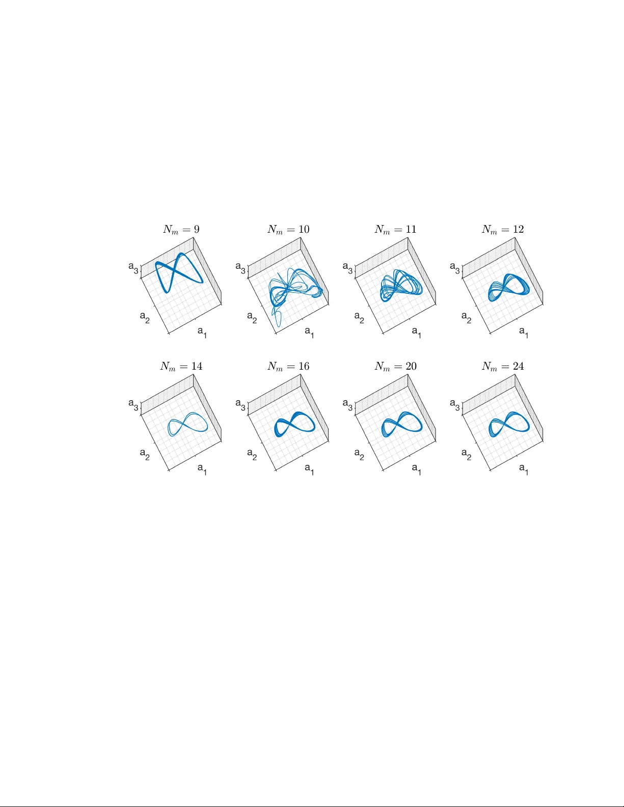
Ho w En tropic Regression Beats the Outliers Problem in Nonlinear System Iden tiﬁcation Ab d AlRahman R. AlMomani 1,2 , Jie Sun 3 , and Erik Bollt 1,2 1 Clarkson Cen ter for Complex Systems Science ( C 3 S 2 ), P otsdam, NY, 13699, USA. 2 Electrical and Computer Engineering, Clarkson Univ ersity , P otsdam, NY, 13699, USA. 3 Theory Lab, Hong Kong Researc h Centre of Hua wei T ec h, Hong Kong, 852, China. Abstract In this w ork, w e developed a nonlinear System Identiﬁcation (SID) method that we called En tropic Regression. Our method adopts an information-theoretic measure for the data-driv en discov ery of the underlying dynamics. Our metho d shows robustness tow ard noise and outliers and it outp erforms many of the curren t state-of-the-art metho ds. Moreo ver, the method of Entropic Regression ov ercomes many of the ma jor limitations of the current metho ds such as sloppy parameters, diverse scale, and SID in high dimensional systems such as complex netw orks. The use of information-theoretic measures in en- tropic regression p oses unique adv an tages, due to the Asymptotic Equipartition Prop ert y (AEP) of probabilit y distributions, that outliers and other lo w-o ccurrence even ts are con venien tly and intrinsically de-emphasized as not-t ypical, b y deﬁnition. W e pro vide a numerical comparison with the current state- of-the-art metho ds in sparse regression, and we apply the methods to diﬀerent c haotic systems such as the Lorenz System, the Kuramoto-Siv ashinsky equations, and the Double W ell P otential. Keyw ords: System Identiﬁcation, Sparse Regression, Data-Driven Modeling, En tropy , Conditional Mu- tual Information, Asymptotic Equipartition Prop erty , Nonlinear dynamics, Complex Systems. System iden tiﬁcation (SID) is a cen tral concept in science and engineering applications whereb y a general mo del form is assumed, but active terms and parameters must b e inferred from observ ations. Most metho ds for SID rely on optimi zing some metric-based cost function that describ es ho w a mo del ﬁts observ ational data. A commonly used cost function emplo ys a Euclidean metric and leads to a least squares estimate, whereas recently it has become p opular to also account for mo del sparsity such as in compressed sensing and Lasso. While the eﬀectiv eness of these metho ds has b een demonstrated in previous studies including in cases where outliers exist in sparse samples, SID remains particularly diﬃcult under more realistic scenarios where each observ ation is sub ject to non-negligible noise, and sometimes ev en contaminated b y large noise outliers. Here w e rep ort that existing sparsit y-fo cused metho ds such as compressiv e sensing, when applied in suc h scenarios, can result in “ov er sparse” solutions that are brittle to outliers. In fact, metric-based metho ds are prone to outliers b ecause outliers by nature hav e an unprop ortionally large inﬂuence. T o mitigate suc h issues of large noise and outliers, we dev elop an en tropic regression approac h for nonlinear SID, whereby true mo del structures are identiﬁed based on an information theoretic criterion describing relev ance in terms of reducing information ﬂow uncertain ty , versus not necessarily (just) sparsit y . The use of information-theoretic measures in entropic regression p oses unique adv an tages, due to the asymptotic equipartition prop erty of probabilit y distributions, that 1 outliers and other lo w-o ccurrence ev ents are con venien tly and intrinsically de-emphasized as not-t ypical, b y deﬁnition. A basic and fundamental problem in science and engineering is to collect data as observ ations from an exp erimen t, and then to attempt to explain the exp eriment b y summarizing data in terms of a mo del. When dealing with a dynamical process, a common scenario is to describe the underlying pro cess as a dynamical system, which ma y b e in the form of a diﬀeren tial equation (DE). T raditionally this means “understanding the underlying physics,” in a manner that allows one to write a DE from ﬁrst principles, including those terms to capture the delicate but imp ortant (physical) eﬀects. V alidation of the mo del ma y come from comparing outputs from the mo del to those from exp eriments, where outputs are typically represen ted as m ultiv ariate time-series. Building a DE mo del based on fundamen tal laws and principles requires strong assumptions, which might b e ev aluated b y ho w the mo del ﬁts data. W eigenbend and Gershenfeld made a distinction betw een w eak mo deling (data rich and theory p o or) and strong mo deling (data p o or and theory ric h), and suggest that it is related to “...the distinction b et ween memorization and generalization...” [ 15 ]. The problem of learning a (dynamical) system from observ ational data is kno wn as system identiﬁc ation (SID), and often times in volv es the underlying assumption that the structur al form of the DE is kno wn (which kinds of terms to include in the functional description of the equation), but only the underlying parameters are not known. F or example, supp ose we observe the dynamics of a simple dissipativ e linear spring, then we ma y express the mo del as m ¨ x + γ ˙ x + k x = 0 based on Hooke’s la w. Ho wev er, the parameters m, γ , and k migh t be unkno wn and need to be estimated in order to completely sp ecify the mo del for purposes suc h as prediction and con trol. One may directly measure those parameters b y static testing (e.g., w eighing the mass on a scale). Alternativ ely , here we are in terested in utilizing the observ ational data generated by the system without ha ving to design and p erform additional exp eriments, to estimate the parameters corresp onding to the mo del that b est ﬁts empirical observ ations, which is a standard viewp oint in SID. In this though t exp erimen t, the SID pro cess is p erformed with the underlying physics understo o d (the form of the Ho ok e spring equation). In general it can b e applied in the scenario where v ery little information is previously kno wn ab out the system, in a blac k b ox manner. Supp ose that observ ations { z ( t ) } come from a general (multidimensional, coupled) DE, represen ted by ˙ z = F ( z ) , (1) where z = [ z 1 , . . . , z N ] T ∈ R N is the (multiv ariate) state v ariable of the system and F = [ F 1 , . . . , F N ] > : R N → R N is the v ector ﬁeld. Each comp onent function F i ( z ) can b e represented using a series expansion (for example a p o wer series or a F ourier series), writing generally , ˙ z i = F i ( z ) = ∞ X k =0 a ik φ k ( z ) , (2) for a linear combination of basis functions { φ k } ∞ k =0 . The basis functions do not need to b e m utually orthog- onal, and the series can ev en include m ultiple bases, for example to con tain b oth a p olynomial basis and a F ourier basis [ 5 ]. The co eﬃcien ts { a ik } are to b e determined by contrasting simulations to exp erimental measuremen ts, in an optimization process whose details of how error is measured distinguishes the v arious metho ds w e discuss here. This w as the main theme in previous approaches on nonlinear SID, with diﬀeren t metho ds diﬀer mainly on how a mo del’s ﬁt is quantiﬁed. The diﬀerent approac hes include using standard squared error measures [ 53 , 9 ], s parsit y-promoting metho ds [ 26 , 5 , 52 , 51 ] as well as using en tropy-based cost functions [ 19 ]. Among those, sparsit y-promoting methods ha ve prov en particularly useful b ecause they tend to av oid the issue of o verﬁtting, thus allowing a large num b er of basis functions to b e included to capture p ossibly ric h dynamical b ehavior [ 26 , 26 , 5 , 52 ]. Regardless of the particular metho d or system, most previous work on nonlinear SID fo cused on the lo w-noise regime and demonstrated success only when there is a suﬃcient amount of clean observ ational data. In practice, an observ ation process can be sub ject to external disturbances in unpredictable w ays. Consequen tly , the eﬀectiv e noise can b e quite large and even with frequently o ccurring “outliers” both of whic h ma y contaminate the otherwise p erfect data. Can SID still w ork under the presence of large noise 2 and outliers? At a glance, the answer should b e yes, given that several recent SID metho ds for nonlinear systems are readily deploy able in the presence of noise. F or example, compressive sensing can handle noise b y relaxing the constraint set whereas least squares and Lasso can b e applied oﬀ the shelf—the imp ortan t question ho wev er is whether the qualit y of solution is compromised or not, and to what exten t. Recently T ran and W ard considered the nonlinear SID problem under the presence of outliers in observ ational data and sho wed that so long as there the outliers are “sparse” leaving suﬃcient amount of “clean” data av ailable, existing tec hniques suc h as SINDy can b e extended to reconstruct the exact form of a system with high probabilit y [ 49 ]. In the curren t w ork, we are interested in the more realistic scenario where eﬀectiv e noise is presen t ev erywhere and th us al l data points are contaminated b y non-negligible noise and sometimes outliers. These features eﬀectiv ely creates a “high noise and low data amount” regime, where we found that existing nonlinear SID metho ds including recent ones that sp ecialize in promoting sparsity , fall short. In this work w e depart from most standard approaches for nonlinear SID. W e identify the error quan- tiﬁcation via me tric-based cost functions as a ro ot cause of existing metho ds to fail under large noise and outliers b ecause outliers tend to deviate from the rest of sample data as measured by metric distance; thus trying to “ﬁt” the outliers almost inevitably causes the model to put (muc h) less weigh ts on the “goo d” data points. T o resolve this imp ortant issue, we prop ose to infer the (sparsit y) structure of a general model together with its parameters using a no vel information the or etic r e gr ession approac h that we call Entropic Regression (ER). As we will show, while standard metric-based metho ds emphasize the data in w ays as designed by the chosen metric, the prop osed ER approach is robust with regards to the presence of noise and outliers in the data. Instead of searc hing for the sparsest mo del and thus risk forcing a wrong sparse mo del, ER is emphasizing “information relev ance” according to a mo del-free, entropic criterion. Basis terms will b e included in the mo del only because they are relev an t and not (necessarily) because they together mak e up the sparsest mo del. W e demonstrate the eﬀectiveness of ER in sev eral examples, including c haotic Lorenz systems, Kuramoto-Siv ashinsky equations, and a double well p oten tial, where in eac h case the ob- serv ed data contains relativ ely large noise and outliers. W e also remark on the computational complexity and con vergence in small-data regime, as w ell as discuss open problems and future directions. Results Nonlinear System Identiﬁcation: Problem Statement and F ormulation F ollowing the standard routine in nonlinear SID [ 34 ], the starting point is to recast the nonlinear SID problem in to a computational inv erse problem, by considering an appropriate set of basis functions that span the space of functions including the system of interest [ 53 , 51 ]. A common c hoice is the standard p olynomial b asis φ = [ φ 0 ( z ) , φ 1 ( z ) , φ 2 ( z ) , . . . ] = [1 , z 1 , z 2 , . . . , z N , z 1 z 2 , z 1 z 3 , . . . , z N − 1 z N , . . . ] (3) where each term is a monomial. Using a set of basis functions, one can represent the individual component functions of F as a series as in ( 2 ). The sp eciﬁcation of the location of nonzero parameters are referred to as the structur e of the mo del. Consider time series data { z ( t ) = [ z 1 ( t ) , . . . , z m ( t )] > } t = t 0 ,...,t ` and corresponding { F ( z ( t ) } t = t 0 ,...,t ` gen- erated from a nonlinear, high-dimensional dynamical system ( 1 ), p ossibly sub ject to observ ational noise. F rom z ( t ), one can estimate the deriv atives by an y of the standard Newton-Cotes metho ds, explicit Euler’s metho d of course b eing the simplest, giving F i ( z ( t k )) = z i ( t k +1 ) − z i ( t k ) τ k + O (( t k +1 − t k )), or cen tral diﬀerence whic h has improv ed accuracy: F i ( z ( t k )) = z i ( t k +1 ) − z i ( t k − 1 ) t k +1 − t k − 1 + O (( t k +1 − t k − 1 ) 2 ). The problem of nonlinear system identiﬁcation is to reconstruct the functional form as w ell as parameters of the underlying system, that is, to infer the nonlinear function F . Under the basis representation ( 2 ), the identiﬁcation of F b ecomes equiv alent to estimating all the parameters { a ik } . In practice, the empirically observed state v ariable is sub ject to noise: ˆ z ( t ) = z ( t ) + η ( t ) with η ( t ) representing the (multiv ariate) noise and ˆ F i denoting the appro ximated v alue of F i . F or noisy observ ations ˆ z ( t ), the diﬀerence betw een ˆ F i ( ˆ z ( t )) and F i ( ˆ z ( t )) originates from several sources: the 3 inﬁnite series is truncated and the deriv ativ es are estimated numerically and b y using appro ximate states. Nev ertheless, w e can represent the aggregated error as an eﬀectiv e noise ξ ( t ) term and express the forward mo del as ˆ F i ( ˆ z ( t )) = K X k =0 a ik φ k ( ˆ z ( t )) + ξ i ( t ) , ( t = t 0 , . . . , t ` ; i = 1 , . . . , N ) . (4) Note that b ecause of the combined and accumulated eﬀects of observ ational noise, approximation error and truncation, even if the observ ational noise of the states η i ( t ) are iid, this is not necessarily true for the eﬀectiv e noise ξ i ( t ). In matrix form, the forward model ( 4 ) has the appro ximate expression   | | | ˙ z 1 ( t i ) . . . ˙ z N ( t i ) | | |   ≈   | | | | φ 0 ( t i ) φ 1 ( t i ) . . . φ K ( t i ) | | | |      a 00 a 01 . . . a 0 N . . . . . . . . . . . . a K 0 a K 1 . . . a K N    . (5) Figure 1 shows the structure of the Lorenz system under standard p olynomial basis up to quadratic terms. Figure 1: (Left) Lorenz system as a dynamical system and its standard graph representation. (Right) Linear com bination of nonlinear basis functions, with coupling co eﬃcien ts { a ik } forming the structure of the system (b ottom right). Here eac h directed edges represent the presence of basis terms on the individual v ariables of the system. In v ector form, under a choice of basis and truncation, the nonlinear system iden tiﬁcation problem can b e recast in to the form of a linear in verse problem f ( i ) = Φ a ( i ) + ξ ( i ) , (6) where f ( i ) = [ ˆ F i ( ˆ z ( t 1 )) , . . . , ˆ F i ( ˆ z ( t ` ))] > ∈ R ` × 1 represen ts the i -th component of the estimated v ector ﬁeld from the observ ational data, Φ = [ φ (1) , . . . , φ ( K ) ] ∈ R ` × K (with φ ( k ) = [ φ k ( ˆ z ( t 1 )) , . . . , φ k ( ˆ z ( t ` ))] ∈ R ` × 1 ) 4 represen t sampled data for the basis functions, ξ ( i ) = [ ξ i ( t 1 ) , . . . , ξ i ( t ` )] > ∈ R ` × 1 represen ts noise, and a ( i ) = [ a i 1 , . . . , a iK ] > ∈ R K × 1 is the vector of parameters whic h is to b e determined. Note that the form of the equation ( 6 ) is the same for eac h i , and solving eac h a ( i ) can be done separately and indep enden tly for each i . In what follows we omit the index when discussing the general metho dology , and consider the follo wing linear inv erse problem f = Φ a + ξ , (7) where f ∈ R ` × 1 and Φ ∈ R ` × K are given, with the goal to estimate a ∈ R K × 1 . This general problem is in the form of an inv erse problem and is typically solved under v arious assumptions of noise by methods suc h as least squares, orthogonal least squares, lasso, compressed sensing, to name a few. Eac h of these metho ds, in addition to the recen t approach of SINDy and its generalization, is men tioned in the Results section and review ed in the Metho ds section. In what follows we dev elop a unique information-theoretic approach called en tropic regression, which w e demonstrate has signiﬁcant adv an tages. En tropic Regression T o ov ercome the competing c hallenges of potential ov erﬁtting, eﬃciency when limited data p oints are given, and robustness with resp ect to noise and in particular outliers in observ ations, we prop ose a nov el frame- w ork that combines the adv an tage of information-theoretic measures and iterativ e regression metho ds. The framew ork, which w e term entr opic r e gr ession (ER), is mo del-free, noise-resilient, and eﬃcient in discov ering a “minimally suﬃcient” mo del to represent data. The key idea is that, for given set of basis functions, a mo del should be considered minimally suﬃcient if no basis function that is not already included in the model can help increase the information relev ance b et ween the mo del outputs and observed data. In other words, the residual betw een the model ﬁt and observ ational data is statistically independent from any basis function that is not included in the model—b ecause otherwise the dependence can b e harv ested to reduce the discrep- ancy by including suc h a basis function in the mo del. W e emphasize that, although the idea seems related to classical mo del selection principles suc h as AIC [ 1 ], ours combines mo del construction with selection. In ad- dition, even though it is not uncommon for entrop y measures to be adopted in system identiﬁcation [ 19 , 37 ], the prop osed method is unique as it fuses entrop y optimization with regression in a principled manner that enables scalable computation and eﬃcien t estimation in reconstruction nonlinear dynamics under noisy data. As w e shall see b elo w, the prop osed ER method is applicable even in the small-sampling regime (b y adopting appropriately deﬁned entrop y measures and eﬃcient estimators) and naturally allo ws for a computationally eﬃcien t procedure to build up a mo del from scratc h. In particular, we use (conditional) mutual information as an information-theoretic criterion and iterativ ely select relev an t basis functions, analogous to the optimal causation entrop y algorithm previously developed for causal netw ork inference [ 47 , 48 ] but here including an additional regression comp onent in eac h step. Th us, ER can b e thought of as an information-theoretic extension of the orthogonal least squares regression, or as a regression version of optimal causation entrop y . W e no w present the details of ER. The ER metho d con tains t wo stages (also see Algorithm 1 for the pseudo code): forward ER and backw ard ER. In b oth stages, selection and elimination are based on an entrop y criterion and parameters are up dated in each iteration using a standard regression (e.g., least squares). Consider the inv erse problem ( 7 ). F or an index set S ⊂ N ∪ { 0 } , the estimated parameters can b e thought of as a mapping from the join t space of Φ, f and S to a vector denoted as ˆ a = R (Φ , f , S ). F or instance, under a least-squares criterion the mapping is given b y R (Φ , f , S ) S = Φ † S f (Φ S denotes the columns of matrix Φ indexed by S ) and R (Φ , f , S ) i = 0 for all i / ∈ S . Using the estimated parameters, the recov ered signal can b e computed as Φ R (Φ , f , S ). In the ER algorithm, we start b y selecting a basis function φ k 1 that maximizes its mutual information with f , compute the corresp onding parameter a k 1 using the least squares metho d, and obtain the corresp onding regression mo del output z 1 according to      k 1 = arg max k I (Φ R (Φ , f , { k } ); f ) , ˆ a = R (Φ , f , k 1 ) , z 1 = Φ R (Φ , f , k 1 ) . (8) 5 Here I ( x ; y ) denotes mutual information b etw een x and y , which is a mo del-free measure of the statistical dep endence b etw een tw o distributions (that is, x and y are indep endent if and only if their m utual informa- tion equals zero) [ 12 ]. Next, in each iteration of the forw ard stage, w e p erform the following computations and up dates, for i = 2 , 3 , . . . ,      k i = arg max k / ∈{ k 1 ,...,k i − 1 } I (Φ R (Φ , f , { k } ); f | z i − 1 ) , ˆ a = R (Φ , f , { k 1 , . . . , k i } ) , z i = Φ R (Φ , f , { k 1 , . . . , k i } ) (9) The process terminates when max k I (Φ R (Φ , f , k ); f | z i − 1 ) ≈ 0 (or when all basis functions are exhausted), indicating that none of the remaining basis function is r elevant given the current mo del, in an information- theoretic sense. The result of the forward ER is a set of indices S = { k 1 , . . . , k m } together with the corresp onding parameters a k 1 , . . . , a k m ( a j = 0 for j / ∈ S ) and mo del f ≈ a k 1 φ k 1 + · · · + a k i φ k i . Finally , we turn to the backw ard stage, where the terms that had previously b een included are re-examined for their information-theoretic relev ance and these that are redundant will b e remov ed. In particular, w e sequentially c heck for eac h j = k i ∈ S to determine if the basis term φ j is redundan t by computing ( ˆ a = R (Φ , f , { k 1 , . . . , k i } / { k i } ) , ¯ z j = Φ R (Φ , f , { k 1 , . . . , k i } / { k i } ) , (10) and up dating S → S/ { j } (that is, remov e j from the set S ) if I (Φ R (Φ , f , S ); f | ¯ z j ) ≈ 0. The result of the bac kward ER is the reduced set of indices S = { ` 1 , . . . , ` n } with n ≤ m , together with the corresp onding parameters a ` 1 , . . . , a ` n ( a j = 0 for j 6∈ S ) computed as a = R (Φ , f , S ), and accordingly the recov ered mo del f ≈ φa = φ S a S = a ` 1 φ ` 1 + · · · + a ` n φ ` n . In practice, mutual information and conditional mutual information need to b e estimated from data, and whether or not the estimated v alues should b e regarded as zero is typically done via (approximate) signiﬁcance testing, the details of which are provided in Metho ds (also see Sec. SI.3 ). Numerical Exp eriments: Outliers, Expansion Order, and the Parado x of Sparsity T o demonstrate the utility of ER for nonlinear system iden tiﬁcation under noisy observ ations, w e b enchmark its p erformance against existing metho ds including least squares (LS), orthogonal least squares (OLS), Lasso, as w ell as SINDy and its extension by T ran and W ard (TW). The details of the existing approac hes are describ ed in the Metho ds Section. The examples we consider represent diﬀeren t types of systems and scenarios, including b oth ODEs and PDEs. In addition, we consider diﬀerent noise mo dels and esp ecially the presence of outliers in order to ev aluate the robustness of the resp ective metho ds. F or eac h example system, we sample the state of each v ariable at a uniform rate of ∆ t to obtain a m ultiv ariate time series { z ( t i ) } k =1 ,...,N ; i =1 ,...,` where z = [ z 1 , . . . , z d ] > ∈ R d ; then we add noise to each state v ariable and obtain the noisy empirical time series denoted by { ˆ z ( t i ) } , where ˆ z k ( t i ) = z k ( t i ) + η ki , (11) with η ki represen ting state observ ational noise. The v ector ﬁeld F is estimated using central diﬀerence on the noisy time series { ˆ z ( t ) } . Example 1. Chaotic Lorenz system. Our ﬁrst detailed example data set was generated by noisy observ ations from a chaotic Lorenz system, which is represented by a three-dimensional ODE which is a protot yp e system as a minimal mo del for thermal con vection obtained by a low-ordered mo dal truncation of the Saltzman PDE [ 41 ], and for man y parameter combinations exhibits c haotic b ehavior [ 35 ]. In our standard notation, we hav e z = [ z 1 , z 2 , z 3 ] > and      ˙ z 1 = F 1 ( z ) = σ ( z 2 − z 1 ) , ˙ z 2 = F 2 ( z ) = z 1 ( ρ − z 3 ) − z 2 , ˙ z 3 = F 3 ( z ) = z 1 z 2 − β z 3 , 6 Algorithm 1 Entropic Regression 1: pro cedure Initializa tion: ( f , Φ ) 2: T olerance ( tol ) Estimation. 3: F or a set of index S , deﬁne the function R (Φ , f , S ) = Φ † S f 4: end pro cedure 5: pro cedure For w ard ER: ( f , Φ , tol ) 6: S f = ∅ , p = ∅ , v = ∞ , z = ∅ 7: while v > tol do 8: S f ← p 9: I est j := I (Φ R (Φ , f , { S f , j } ); f | z ). for all j / ∈ S f 10: v , p := max j I est j 11: ˆ a := R (Φ , f , { S f , p } )) 12: z := Φ ˆ a 13: end while 14: return S f 15: end pro cedure 16: pro cedure Backw ard ER: ( f , Φ , tol , S f ) 17: S b = S f , p = ∅ , v = −∞ 18: while v < tol do 19: S b := { S b } − { p } 20: for all j ∈ S b do 21: ˆ a := R (Φ , f , { S b } − { j } )) 22: z := Φ ˆ a 23: I est j := I (Φ R (Φ , f , S b ); f | z ), 24: end for 25: v , p := min j ( I est j ) 26: end while 27: return S b 28: end pro cedure 29: return S = S b . 7 Figure 2: Lorenz system. W e p erform 100 runs for the comparison, no outliers, 0.0005 step size, and w e considered the median result out of 100 runs. The ﬁgure shows the error in the parameter estimation for a Lorenz system but sub ject to noisy measuremen ts by Gaussian noise, with  = 10 − 4 , and using a 5 th -order p olynomial expansion. W e see that ER and OLS has an o verall superior p erformance compared to others standard methods. W e see that SINDy , and TW are less successful (under large span of tuning parameters, see Fig.( SI.13 )) at this num b er of measurements ev en with low noise levels. with default parameter v alues σ = 10, ρ = 28 and β = 8 / 3 unless otherwise speciﬁed. W e consider a standard p olynomial basis as in Eq. ( 3 ). Ov er recen t y ears, the Lorenz system has become a fav orable and standard example for testing SID metho ds and typically requires tens of thousands of measuremen ts for accurate reconstruction [ 49 , 5 ]. First, w e compare sev eral nonlinear SID metho ds in reconstructing the Lorenz system when the state observ ational noise is dra wn indep enden tly from a Gaussian distribution, η ∼ N (0 ,  2 ). As w e discussed b efore, this translates in to eﬀectiv e noise that is not necessarily Gaussian or ev en indep endent. Fig. 2 sho ws the error in the estimated parameters where, err or = k a true − a estimated k 2 . As shown in Fig. 2 , even with observ ational noise as low as  = 10 − 4 , ER and OLS outperform all other metho ds. In this low noise regime, SINDy required more measurements (around 4 times) to reach similar accuracy as ER. In comparison, as noted in [ 49 , 5 ] and in the implemen tation pro vided b y the authors, for SINDy and TW metho ds to yield accurate reconstruction the num ber of measuremen ts is at the order of 10 4 . Next, to explore the p erformance of SID metho ds under the presence of outliers, we conduct additional n umerical exp erimen ts. The extent to whic h outliers presen t is con trolled b y a single parameter p : each observ ation is sub ject to an added noise η , where η ∼ N (0 ,  2 1 ) with probabilit y 1 − p and η ∼ N (0 ,  2 1 +  2 2 ) with probability p . Here w e use  1 = 10 − 5 ,  2 = 0 . 2 and p = 0 . 2. The results of SID are shown in Fig. 3 . Compared to Fig.( 2 ), w e see that with p > 0 OLS p erformance drops due to the increasing o ccurrence of large noise and outliers whereas ER remains its capacit y of accurately identifying the underlying system. As an example, in each of the side panels of Fig. 3 , we show the tra jectory of the identiﬁed dynamics using the median solution of each metho d. It is clear that under suc h noisy chaotic dynamics and at a relatively under-sampled regime, ER metho d successfully reco vers the system dynamic. As an ample amount of data b ecomes av ailable, we note that TW metho d starts to pro duce excellent reconstruction whic h is consisten t with recen t ﬁndings rep orted in Ref. [ 49 ]. Giv en that a ma jor theme of mo dern SID is to seek for sp arse representations, and the Lorenz system under standard p olynomial basis is indeed sparse, it is worth asking: what are the resp ective structure iden tiﬁed by the diﬀerent metho ds? In Fig. 4 we compare the structure of the iden tiﬁed mo del using diﬀeren t metho ds across a range of parameter v alues for ρ . In this case, under the presence of large noise and outliers ( p = 0 . 2), none of the metho ds examined here, including recently prop osed sparsit y-promoting (CS, SINDy) and outlier-resilien t (TW) metho ds, is able to identify the correct structure. The prop osed ER metho d, 8 Figure 3: SID for the Lorenz system when the observ ations are corrupted b y outliers. Contrast to Fig. 2 . As b efore, we sp ecify a lev el of p ersistent Gaussian observ ation noise, η ∼ N (0 ,  1 )(1 − B er ( p )), but now furthermore we allo w for an “outlier noise”, as “occasional” bursts of muc h larger p erturbations, η ∼ N (0 ,  1 +  2 ) B er ( p ), where B er ( p ) is the standard Bernoulli random v ariable (0 or 1 with probability ratio p , and 0 ≤ p ≤ 1). (Middle) Error in estimated parameters for Lorenz system given in Eq. 12 with noise,  1 = 10 − 5 ,  2 = 0 . 2, 5 th -Order p olynomial expansion, and p = 0 . 2. Lorenz system dynamics is sho wn in the upp er right corner. W e see that ER has fast conv ergence at a lo w num b er of m easuremen ts, follow ed by TW whic h required twice num b er of measuremen ts. Diﬀerent from TW, in our ER metho d we fo cus in detecting the true sparse structure with the presence of outliers, without any attempts to neglect outliers based on some w eight function to ac hiev e higher accuracy which is the case in TW method. This p oint clearly app ears in Fig.( SI.14 where we see that although TW achiv ed higher accuracy , it has lo w exact recov ery probability , while ER reac hed exact recov ery probability more than 90%. A detailed statistics b o x-plot (quartiles, median,...,etc) ov er the 100 runs with 1500 measurements is sho wn in Fig. ( SI.15 ). (Side panels) T ypical tra jectories generated by the reconstructed dynamical systems, where for each method we sho w results using the “median” solution, that is, recov ered system whose corresp onding parameter estimation error is at the median ov er a large num b er of indep endent sim ulation runs. In each such simulation, 1500 samples are used. Comparing with the true Lorenz attractor (upp er right corner in the main panel), we see that the only reasonable reconstruction in this case was pro duced by ER. 9 Figure 4: Sparse representation of the solution found by solv ers using 1500 measurements, and p = 0 . 2 on Fig.( 3 ). The upp er left corner sho ws the true solution of Lorenz system. The b ottom column sho ws the bifurcation diagram on z dimension of Lorenz system with ρ ∈ [5 , 30] as bifurcation parameter, created using 5000 initial conditions evolv ed according the reco vered solution. ho wev er, do es iden tify the correct structure. It is worth p ointing out that, often times when expressed in the right basis, a mo del will app ears to b e sparse, the conv erse is not true: just b ecause a metho d return a sparse solution do es not suggest (at all) the suc h a solution gives a reasonable approximation of the true mo del structure. Interestingly , as we show in Fig. SI.1 and Fig. SI.2 , for the same system and data, as more basis functions are used–that is, when the true dynamics b ecomes sparser–the reconstructed dynamics using existing metho ds (suc h as CS) can become worse. Example 2. Kuramoto-Siv ashinsky equations. T o further demonstrate the p o wer of ER, w e consider a nonlinear PDE, namely the Kuramoto-Siv ashinsky (KS) equation [ 32 , 31 , 45 , 22 , 33 ], which arises as a description of ﬂame fron t ﬂutter of gas burning in a cylindrically symmetric burner. It has b ecome a p opular example of a PDE that exhibits chaotic b ehavior, in particular spatiotemporal chaos [ 11 , 21 ]. W e will consider Kuramoto-Siv ashinsky system in the follo wing form, u t = − ν u xxxx − u xx + 2 uu x , ( t, x ) ∈ [0 , ∞ ) × (0 , L ) (12) in p erio dic domain, u ( t, x ) = u ( t, x + L ), and w e restrict our solution to the subspace of o dd solutions u ( t, − x ) = − u ( t, x ). The viscosity parameter ν con trols the suppression of solutions with fast spatial v ariations, and is set to ν = 0 . 029910 under which the system exhibit c haotic b ehavior [ 11 ]. Since a PDE corresponds to an inﬁnite-dimensional dynamical system, in practice we fo cus on an ap- pro ximate ﬁnite-dimensional representation of the system, for example, by Galerkin-pro jection onto basis 10 functions as inﬁnitely many ODE’s in the corresp onding Banach space. T o develop the Galerkin pro jection, we follow the pro cedure as presented in [ 13 ], to expand a p eriodic solution u ( x, t ) using a discrete spatial F ourier series, u ( x, t ) = ∞ X −∞ b k ( t ) e ikq x , where q = 2 π L . (13) Notice that we hav e written this F ourier series of basis elements e ikq x in terms of time v arying combinations of basis elemen ts. F or simplicity , consider L = 2 π , then q = 1 for the follo wing analysis. This is typical [ 40 ] with the representation of a PDE as inﬁnitely man y ODE’s in the Banach space, where orbits of these co eﬃcien ts therefore b ecome time v arying patterns b y Eq. ( 13 ). Substituting Eq. ( 13 ) in to Eq. ( 12 ), we pro duce the inﬁnitely man y evolution equations for the F ourier co eﬃcients, ˙ b k = ( k 2 − ν k 4 ) b k + ik ∞ X m = −∞ b m b k − m (14) In general, the coeﬃcients b k are complex functions of time t . How ev er, by symmetry , we can reduce to a subspace by considering the sp ecial symmetry case that b k is pure imaginary , b k = ia k and a k ∈ R . Then, ˙ a k = ( k 2 − ν k 4 ) a k − k ∞ X m = −∞ a m a k − m . (15) where k = 1 , .., N m . How ev er, the assumption that there is a slo w manifold (slow modes as an inertial manifold [ 40 , 24 , 38 , 25 ]) suggests the practical matter that a ﬁnite truncation of the series Eq. ( 13 ), and corresp ondingly the a reduction to ﬁnitely man y ODEs will suﬃce. Therefore w e choose a suﬃcien tly large n umber of mo des N m . Then we solve the resulting N m -dimensional ODE ( 15 ) to pro duce the estimated solution of u ( x, t ) by ( 13 ), and use suc h data for the purpose of SID, hav e meaning to estimate the structure and parameters of the ODE mo del ( 15 ). Fig. 5 sho ws the ﬁrst three dimensions plot under diﬀerent num b er of mo des. W e see that using just a few n umber of mo des ( N m = 8 , ..., 11) is insuﬃcient to capture the true dynamical b eha vior of the system whereas too large a num b er of mo des ( N m = 20 , 24) ma y b e unnecessary . In this example, an adequate but not excessiv e num b er of modes seems to b e around N m = 16, as no signiﬁcan t information is gained by increasing N m . Fig. 6 shows the sparse structure of the recov ered solution b y diﬀeren t metho ds. Here w e men tion that the true non-zero parameters of KSE using N m = 16 are 200 parameters that v ary in the magnitude from 0.9701 to 1705. With the second order expansion, our basis matrix will ha ve 153 candidate functions, and it will b e nearly singular with condition n umber 4 × 10 7 . Likely due to such high condition n umber, neither TW nor SINDy gives reasonable reconstruction. In particular, w e note that the solution of SINDy is already optimized by selecting the threshold v alue λ that is sligh tly abov e λ ∗ where here λ ∗ ≈ 0 . 1731 is the smallest magnitude of the true nonzero parameter of the full least squares solution. A larger v alue of λ only worsens the reconstruction, as we found numerically . The OLS metho d ov ercomes the disadv an tage of LS by iterativ ely ﬁnding the most relev ant “feature” v ariables, where relev ance is measured in terms of (squared) mo del error; but it comes at a price: similar to LS, the OLS is sensitiv e to outliers in the data and suc h sensitivity seems to b e even more ampliﬁed due to the smaller n umber of terms typically included in OLS as compared to LS, which cause the high false negativ e rate in the OLS solution. Although ER solution has few false negatives, but was completely able to reco ver the ov erall dynamic of the system as shown in Fig.( 7 ), while all other solutions div erges and failed to reco ver u ( x, t ). Example 3. Double W ell Poten tial. Finally , in order to gain further insights into wh y standard methods fail under the presence of outliers, we consider a relativ ely simple double-well system, with f ( x ) = x 4 − x 2 . (16) 11 Figure 5: The ﬁrst three mo des of the ODE Eq.( 15 ) solution. W e sho w the mo des a 1 , a 2 and a 3 for selected n umber of modes. F or clear view, we ﬁxed the axis limits to b e a 1 ∈ [ − 1 . 21 , 1 . 06] , a 2 ∈ [ − 0 . 75 , 0 . 98] and a 3 ∈ [ − 1 . 1 , 1 . 12] for all plots. W e found that there was no signiﬁcan t addition to the dynamic with 16 < N m . (meaning that N m = 16 w as enough to describe the system). 12 Figure 6: In analogy to Fig. 4 , sparse representation of KSE solution by diﬀeren t metho ds. CS, LASSO hav e b een excluded for their high computation complexity . Supp ose that we measure x and f , can w e iden tify the function f ( x )? W e sample 61 equally spaced mea- suremen ts for x ∈ [ − 1 . 2 , 1 . 2], and we construct Φ using the 10 th order p olynomial expansion with K = 11 is the num b er of candidate functions. Then, w e consider a single ﬁxed v alue corrupted measurement to b e f (0 . 6) = 0 . 2. Fig. 8 shows the results the double-well SID under a single outlier in the observ ation. W e see the robustness of ER solution to the outliers while CS failed in detecting the system sparse structure. F or the sak e of clearness, Fig. 8 shows the results for CS and ER. The results for each solv er and details are provided in Sec. ( SI.4.1 ) in addition to more numerical examples. Discussion The main theme of the pap er is on nonlinear system identiﬁcation (SID) under noisy observ ations, whic h is to learn the functional form and parameters of a nonlinear system based on observ ations of its states under the presence of noise and outliers. W e recast the problem in to the form of an inv erse problem using a basis expansion of the nonlinear functions. Such basis expansion, ho wev er, renders the resulting problem inherently high dimensional even for lo w-dimensional systems. In practice, the need for ﬁnite-order truncation as well as the presence of noise causes additional c hallenges. F or instance, even under iid Gaussian observ ational noise for the state v ariables, the eﬀectiv e noise in the in verse problem is not necessarily so. As we demonstrate using several example systems, including the chaotic Lorenz system and the Kuramoto-Siv ashinsky equations, existing SID metho ds are prone to noise, and can b e quite sensitiv e to the presence of outliers. W e identify the ro ot cause of suc h non-robustness b eing the metric nature of the existing metho ds, as they quantify error based on metric distance, and th us a handful of data p oin ts that are “corrupted” b y large noise can dominate the model ﬁt. Eac h of the existing methods we considered has this property , which includes the least squares, compressiv e sensing, and Lasso. F rom a mathematical p oint of view, eac h metho d can b e interpreted as a functional that maps input data to a mo del, through some optimization pro cess. In a noisy setting, the output mo del should ideally change smo othly with resp ect to the input data, not just con tinuously . Our results suggest that these p opular metho ds in fact do suﬀer from a sensitive dep endence on outliers, as a few corrupted data can already pro duce very p o or mo del estimates. Alarmingly , the now-popular CS metho d, whic h is based on sparse regression, can force to select a completely wrong sparse mo del under noisy input data, and this o ccurs even when there is just a single outlier. This is by no means contradicting previous ﬁndings of the success of CS in SID, as in suc h work noise is t ypically v ery small, and here we are considering 13 Figure 7: u ( x, t ) constructed b y the true solution (left) and the ER solution (right) using Eq.( 13 ). OLS and TW w as not able to re-produce the dynamic and they div erge after few iterations. w e see that the reconstructed dynamic using ER solution is iden tical to the true solution with a minor diﬀerence in the transien t time, although there w as a false negativ e in the ER solution. ER detected the stiﬀ parameters that dominate the ov erall dynamic. Sloppiness of some KSE parameters mak e there inﬂuence practically negligible to the ov erall dynamic. 14 Figure 8: Double well potential giv en by Eq. ( 16 ) data ﬁtting using ER and CS. CS solution found as the solution with minimum residual from 100 log-spaced v alues of  ∈ [10 − 9 , 10 2 ]. a p erhaps more realistic scenario with larger noise. T o ﬁll the v acancy of SID metho ds that can o vercome outliers, we dev elop an information-theoretic regression technique, called entropic regression (ER), that combines en tropy measures with an iterative optimization for nonlinear SID. W e sho w that ER is robust to noise and outliers, in the otherwise very c hallenging circumstances of ﬁnding a mo del that explains data from dynamical sto c hastic pro cesses. The k ey to ER’s success is its abilit y to recov er the correct and true sparsit y structure of a nonlinear system under basis expansions, despite either relatively large noise, or alternatively ev en relatively man y even larger outliers. In this sense ER is sup erior to an y other metho d that we know of for suc h settings. Note that in the ER algorithm, least squares is used to estimate the parameters of those basis functions that are deemed relev an t where relev ance is detected using an information-theoretic measure that is insensitiv e to noise and outliers. The choice of least squares in the regression step in ER is not necessarily an optimal choice and can b e potentially replaced by more adv anced metho ds (e.g., those developed in robust regression). In the current implementation of ER we adopted least squares mainly due to its computational adv an tage o ver alternativ e metho ds. On a more fundamen tal level, ER’s robustness against outliers ma y likely be attributed to an important principle in information theory called the asymptotic equipartition prop erty (AEP) [ 12 ]. The outcome of this principle is that sampled data can b e partitioned in to “t ypical” samples and “atypical” samples, with the rare atypical samples end up inﬂuencing the estimated entrop y relatively w eakly . Since ER measures relev ance by entrop y instead of metric distance, a few outliers, no matter how far aw a y they are from the rest of the data p oints, tend to hav e minimal impact on the mo del identiﬁcation process. So the general in terpretion we make here is that outliers observ ations are likely at ypical, but not part of the core of data that carry the ma jor estimation of the en tropy . This foundational concept of information theory is lik ely the ma jor source of robustness of our ER method to system iden tiﬁcation. 15 Metho ds Existing metric-based metho ds for system identiﬁcation Recall (from the main text) that we recast the nonlinear system iden tiﬁcation problem here. Giv en a truncated basis representation of each component of the v ector ﬁeld F , expressed as F i ( z ) = K X k =0 a ik φ k ( z ) , (17) w e consider sampled data ˆ z and the estimated vector ﬁeld ˆ F , from which the co eﬃcients (parameters) { a ik } are to b e determined. In general, we use subscript “ t ” to index the sampled data, and thus the t -th sample satisﬁes the equation ˆ F i ( ˆ z ( t )) = K X k =0 a ik φ k ( ˆ z ( t )) + ξ i ( t ) , ( t = 1 , . . . , T ; i = 1 , . . . , n ) . (18) Here ξ i ( t ) is the eﬀectiv e noise that represents the accum ulative impact of truncation error, state observ a- tional noise as w ell as approximation error in the estimation of deriv ativ es. Consequen tly , an iid Gaussian noise additiv e to the states z i ( t ) can translate into correlated non-Gaussian eﬀective noise for ξ i ( t ). Ha ving transformed a system identiﬁcation problem into an parameter estimation problem (or inv erse problem) in the form of f ( i ) = Φ a ( i ) + ξ ( i ) , (19) where f ( i ) = [ ˆ F i ( ˆ z (1)) , . . . , ˆ F i ( ˆ z ( T ))] > ∈ R T × 1 represen ts the estimated function F i ( i -th comp onent of the v ector ﬁeld F ), Φ = [ φ (1) , . . . , φ ( K ) ] ∈ R T × K (with φ ( k ) = [ φ k ( ˆ z (1)) , . . . , φ k ( ˆ z ( T ))] ∈ R T × 1 ) represen t sampled data for the basis functions, ξ ( i ) = [ ξ i (1) , . . . , ξ i ( T )] > ∈ R T × 1 represen ts eﬀective noise, and a ( i ) = [ a i 1 , . . . , a iK ] > ∈ R K × 1 is the vector of parameters which is to b e determined. Since the form of the equation ( 19 ) is the same for eac h i , w e omit the index when discussing the general metho dology , and consider the following linear inv erse problem f = Φ a + ξ , (20) where f ∈ R T × 1 and Φ ∈ R T × K are given, with the goal is to estimate a ∈ R K × 1 when the eﬀective noise is not necessarily from indep endent multiv ariate Gaussian distribution. Least Squares (LS) The most commonly used approach to estimate a in Eq. ( 20 ) is to use the least squares criterion, which ﬁnds a b y solving the follo wing least squares minimization problem: min a ∈ R K k Φ a − f k 2 . (21) The solution can b e explicitly computed, giving a (LS) = Φ † f , (22) where Φ † denotes the pseudoin verse of the matrix Φ [ 16 ]. Note that in the sp ecial case where the minimum is zero (which is unlikely under the presence of noise), the minimizer is not unique and the “least-squares” solution typically refers to a vector a that has the minimal 2-norm and solves the equation Φ a = f . The LS metho d has sev eral adv antages: it is analytically traceable and easy to solve computationally using standard linear algebra routines (e.g., SVD). How ever, a main disadv an tage of the LS approac h in system iden tiﬁcation, as we discuss in the main text, is that it generally pro duces a “dense” solution, where most (if not all) components of a are nonzero, which is a severe ov erﬁtting of the actual mo del. This (undesired) feature also makes the metho d sensitive to noise, especially in the under-sampling regime. 16 Orthogonal Least Squares (OLS) In orthogonal least squares (OLS) [ 9 , 50 , 29 ], the idea is to iteratively select the columns of Φ that minimize the (2-norm) mo del error, which corresp onds to iterative assigning nonzero v alues to the comp onents of a . In particular, the ﬁrst step is to select basis φ k 1 and compute the corresp onding parameter a k 1 and residual r 1 according to ( ( k 1 , a k 1 ) = arg min k,c k f − c φ k k 2 , r 1 = f − φ k 1 a k 1 . (23) Then, one iterativ ely selects additional basis functions (un til stopping cretia is met) and compute the corre- sp onding parameter v alue and residual, as ( ( k ` +1 , a k ` +1 ) = arg min k,c k r ` − c φ k k 2 , r ` +1 = r ` − φ k ` +1 a k ` +1 . (24) As for stopping criteria, there are several c hoices including AIC and BIC. In this w ork, in the absence of kno wledge of the error distribution, w e adopt a commonly used criterion where the iterations terminate when the norm of the residual is b elo w a prescrib ed threshold. T o determine the threshold, we consider 50 log-spaced candidate v alues in the in terv al [10 − 6 , 100] and select the best using 5-fold cross v alidation. Lasso A principled wa y to imp ose sparsity on the mo del structure is to explicitly penalize solution vectors that are non-sparse, b y formulating a regularized optimization problem: min a ∈ R K  k Φ a − f k 2 2 + λ k a k 1  , (25) where the parameter λ ≥ 0 con trols the extent to whic h sparsit y is desired: as λ → ∞ the second term dominates and the only solution is a vector of all zeros, whereas at the other extreme λ = 0 and the problem b ecomes identical to a least squares problem whic h generally yields a full (non-sparse) solution. V alues of λ in betw een then balances the “model ﬁt” quantiﬁed by the 2-norm and the sparsit y of the solution c haracterized by the 1-norm. F or a given problem, the parameter λ needs to b e tuned in order to sp ecify a particular solution. A common wa y to select λ is via cross v alidation [ 20 ]. In our numerical exp erimen ts, w e c ho ose λ span according to [ 20 ], with 5-F olds cross v alidation and 10 v alues λ span. W e adopt the CVX solv er [ 18 ], and from all the solutions found for eac h λ we select the solution with minimum residual. Compressed sensing (CS) Originally developed in the signal pro cessing literature [ 8 , 7 , 14 ], the idea of compressed sensing (CS) has b een adopted in several recent work in nonlinear system iden tiﬁcation [ 52 , 51 ] Under the CS framew ork, one solv es the following constrained optimization problem, ( arg min a k a k 1 , sub ject to k Φ a − f k ≤ , (26) where the parameter  ≥ 0 is used to relax the otherwise strict constraint Φ a = f , to allow for the presence of noise in data. In our n umerical exp eriments, we choose 10 log-spaced v alues for  ∈ [10 − 6 , 100], and 5-F olds cross v alidation. W e adopt the CVX solver [ 18 ], and from all the solutions found for eac h  we select the solution with minimum residual. 17 SINDy In their recent con tribution, Brun ton, Pro ctor and Kutz introduced SINDy (Sparse Iden tiﬁcation of Nonlinear Dynamics) as a wa y to perform nonlinear system iden tiﬁcation [ 5 ]. Their main idea is, after form ulating the inv erse problem ( 20 ), to seek a sp arse solution. In particular, given that Lasso can b e computationally costly , they prop osed to use sequential least squares with (hard) thresholding as an alternative. F or a (prec hosen) threshold λ , the metho d starts from a least squares solution and abandons all basis functions whose corresp onding parameter in the solution has absolute v alue smaller than λ ; then the same is rep eated for the data matrix asso ciated with the remaining basis functions, and so on and so forth, until no more basis function (and the corresp onding parameter) is remov ed. F or fairness of comparison, we present results of SINDy according to the b est threshold parameter λ manually c hosen so that no active basis function is remo ved in the very ﬁrst step (see KSE example); for the Lorenz system example, we choose λ = 0 . 02 as used in a similar example as in Ref. [ 5 ]. T ran-W ard (TW) In their recent pap er [ 49 ] T ran and W ard considered the SID problem where certain fraction of data p oints are corrupted, and prop osed a metho d to simultaneously identify these corrupted data and reconstruct the system assuming that the corrupted data o ccurs in sparse and isolated time interv als. In addition to an initial guess of the solution and corresp onding residual, which can b e assigned using standard least squares, the TW approac h requires a pre-determiniation of three additional parameters: a tolerance v alue to set the stopping criterion, threshold v alue λ used in each iteration to set those parameters whose absolute v alues are b elow λ to be zero, and another parameter µ to con trol the exten t to which data p oin ts that do not (appro ximately) satisfy the prescribed mo del are to b e considered as “corrupted data” and remov ed. F or the Lorenz system example, we used the same parameters as in Ref. [ 49 ] whereas for the KSE example, we ﬁx µ = 0 . 0125 (the same used in Ref. [ 49 ] and select λ similarly as for the implementation of SINDy . Implemen tation Details of Entropic Regression (ER) As describ ed in the main text, and as shown in details in Algorithm ( 1 ), a key quantit y to compute in ER is the conditional mutual information I ( X ; Y | Z ) among three (p ossibly m ultiv ariate) random v ariables X , Y and Z via samples from these v ariables, denoted by ( x t , y t , z t ) t =1 ,...,T . Since the distribution of the v ariables and their dep endences are generally unkno wn, w e adopt a nonparametric estimator for I ( X ; Y | Z ) which is based on statistics of k nearest neighbors [ 30 ]. W e ﬁx k = 2 in all of the rep orted numerical exp erimen ts; w e ha ve found that the results change quite minimally when k is v aried from this ﬁxed v alue, suggesting relativ e robustness of the method. Another important issue in practice is the determination of threshold under which the conditional m utual information I ( X ; Y | Z ) should b e regarded zero. In theory I ( X ; Y | Z ) is alwa ys nonnegative and equals zero if and only if X and Y are statistically indep endent giv en Z , but such absolute criterion needs to b e softened in practice b ecause the estimated v alue of I ( X ; Y | Z ) is generally nonzero even when X and Y are indeed indep enden t given Z . A common wa y to determine whether I ( X ; Y | Z ) = 0 or I ( X ; Y | Z ) > 0 is to compare the estimated v alue of I ( X ; Y | Z ) against some threshold. See Sec. ( SI.3 ) for details of robust estimation of the threshold in the context of SID. Supplemen tary Material See supplemen tary material for more details in information theory measures, and additional n umerical results for the double-well p otential, Lorenz system, and a coupled net work of the logistic map. 18 Ac kno wledgemen ts This work w as funded in part by the Simons F oundation Grant No. 318812, the Army Researc h Oﬃce Grant No. W911NF-16-1-0081, the Oﬃce of Nav al Research Gran t No. N00014-15-1-2093, and also D ARP A. References [1] Hirotogu Ak aike. A new lo ok at the statistical mo del iden tiﬁcation. IEEE T r ansactions on Automatic Contr ol , 19(6):716–723, 1974. [2] Celia Anteneodo, An tonio Marcos Batista, and Ricardo L. Viana. Synchronization threshold in coupled logistic map lattices. Physic a D: Nonline ar Phenomena , 223(2):270 – 275, 2006. [3] Erik Bollt. A ttractor Mo deling and Empirical Nonlinear Mo del Reduction of Dissipative Dynamical Systems. International Journal Of Bifur c ation A nd Chaos , 17(4):1199–1219, 2007. [4] Steve Brun ton. Kutz Research Group W ebsite. Op en source co de. Matlab Co de for SINDy as of F eb 28, 2018. https://facult y .washington.edu/sbrun ton/sparsedynamics.zip. [5] Steven L. Brunton, Josh ua L. Pro ctor, and J. Nathan Kutz. Disco vering gov erning equations from data b y sparse identiﬁcation of nonlinear dynamical systems. Pr o c e e dings of the National A c ademy of Scienc es , 113(15):3932–3937, 2016. [6] Steven L. Brunton, Joshua L. Pro ctor, Jonathan H. T u, and Nathan Kutz. Compressed sensing and dynamic mo de decomp osition. Journal of Computational Dynamics , 2(2158 2491 2015 2 165):165, 2015. [7] Emmanuel J. Cand ` es, Justin Romberg, and T erence T ao. Robust uncertaint y principles: Exact sig- nal reconstruction from highly incomplete frequency information. IEEE T r ansactions on Information The ory , 52(2):489–509, 2006. [8] Emmanuel J. Cand ` es, Justin K. Romberg, and T erence T ao. Stable signal reco very from incomplete and inaccurate measuremen ts. Communic ations on Pur e and Applie d Mathematics , 59(8):1207–1223, 2006. [9] Sheng Chen, Stephen A. Billings, and W an Luo. Orthogonal least squares metho ds and their application to non-linear system identiﬁcation. International Journal of Contr ol , 50(5):1873–1896, 1989. [10] Y u-Zhong Chen and Ying-Cheng Lai. Sparse dynamical b oltzmann machine for reconstructing complex net works with binary dynamics. Physic al R eview E , 97:032317, Mar 2018. [11] F reddy Christiansen, Predrag Cvitanovic, and V akhtang Putk aradze. Spatiotemporal c haos in terms of unstable recurren t patterns. Nonline arity , 10(1):55, 1997. [12] Thomas M. Co ver and Jo y A. Thomas. Elements of Information The ory . Hoboken, NJ Wiley- In terscience, 2005. [13] Predrag Cvitanovic, Rob erto Artuso, Ronnie Mainieri, Gregor T anner, G´ ab or V atta y , Niall Whelan, and Andreas Wirzba. Chaos: classical and quan tum. ChaosBo ok. or g (Niels Bohr Institute, Cop enhagen 2005) , 69, 2005. [14] David L. Donoho. Compressed sensing. IEEE T r ansactions on Information The ory , 52(4):1289–1306, April 2006. [15] Neil A. Gershenfeld and Andreas S. W eigend. The futur e of time series. Time Series Pr e diction: F or e- c asting the F utur e and Understanding the Past . Addison-W esley , 1993. [16] Gene H. Golub and Charles F. V an Loan. Matrix Computations (4th Ed.) . Johns Hopkins Univ ersity Press, Baltimore, MD, USA, 2013. ISBN: 1-4214-0859-7. 19 [17] Clive Granger. In vestigating Causal Relations by Econometric Mo dels and Cross-sp ectral Methods. Ec onometric a , 37(3):424–438, 1969. [18] Michael Grant and Stephen Bo yd. CVX: Matlab soft ware for disciplined conv ex programming, 2008. [19] Ling-zhong Guo, Stephen A Billings, and DQ Zhu. An extended orthogonal forward regression algorithm for system identiﬁcation using entrop y . International Journal of Contr ol , 81(4):690–699, 2008. [20] T revor Hastie, Rob ert Tibshirani, and Martin W ainwrigh t. Statistic al le arning with sp arsity: The lasso and gener alizations . CR C Press, 2015. [21] Pierre Hohen b erg and Boris Shraiman I. Chaotic b ehavior of an extended system. Physic a D: Nonline ar Phenomena , 1989. [22] James M. Hyman and Basil Nicolaenko. The kuramoto-siv ashinsky equation: A bridge betw een p de’s and dynamical systems. Physic a D: Nonline ar Phenomena , 18(1):113 – 126, 1986. [23] Sarik a Jalan, RE Amritk ar, and Chin-Kun Hu. Sync hronized clusters in coupled map net works. i. n umerical studies. Physic al R eview E , 72(1):016211, 2005. [24] Michael S. Jolly , Ioannis Kevrekidis, and Edriss S. Titi. Appro ximate inertial manifolds for the Kuramoto-Siv ashinsky equation: analysis and computations. Physic a D: Nonline ar Phenomena , 44(1- 2):38–60, 1990. [25] Michael S. Jolly , Ricardo M. S. Rosa, and Roger M. T emam. Accurate computations on inertial mani- folds. Physics L etters A , 131:433–436, 2001. [26] Nicholas Kalouptsidis, Gerasimos Mileounis, Beh tash Babadi, and V ahid T arokh. Adaptiv e algorithms for sparse system identiﬁcation. Signal Pr o c essing , 91(8):1910 – 1919, 2011. [27] Kunihiko Kanek o. Overview of coupled map lattices. Chaos: A n Inter disciplinary Journal of Nonline ar Scienc e , 2(3):279–282, 1992. [28] F Kaspar and HG Sch uster. Easily calculable measure for the complexit y of spatiotemp oral patterns. Physic al R eview A , 36(2):842, 1987. [29] Michael Korenberg, Stephen A. Billings, Huanzhao Liu, and P .J. McIlroy . Orthogonal parameter es- timation algorithm for non-linear sto c hastic systems. International Journal of Contr ol , 48(1):193–210, 1988. [30] Alexander Krask o v, Harald St¨ ogbauer, and P eter Grassb erger. Estimating mutual information. Physic al R eview E , 69:066–138, Jun 2004. [31] Y oshiki Kuramoto. Diﬀusion-Induced Chaos in Reaction Systems. Pr o gr ess of The or etic al Physics Supplement , 64:346–367, 02 1978. [32] Y oshiki Kuramoto and T oshio Tsuzuki. Persisten t Propagation of Concentration W av es in Dissipative Media F ar from Thermal Equilibrium. Pr o gr ess of The or etic al Physics , 55(2):356–369, 02 1976. [33] Y ueheng Lan and Predrag Cvitanovi ´ c. Unstable recurren t patterns in kuramoto-siv ashinsky dynamics. Physic al R eview E , 78:026208, Aug 2008. [34] Lennart Ljung. System identiﬁcation. Wiley Encyclop e dia of Ele ctric al and Ele ctr onics Engine ering , pages 1–19, 1999. [35] Edward N. Lorenz. Deterministic nonp erio dic ﬂow. Journal of the Atmospheric Scienc es , 20(2):130–141, 1963. 20 [36] Cristina Masoller, Italo Herb ert Lucena Cav alcante, and Jose Rob erto Rios Leite. Dela yed coupling of logistic maps. Physic al R eview E , 64(3):037202, 2001. [37] Giulia Prando, Alessandro Chiuso, and Gianluigi Pillonetto. Maximum en tropy v ector kernels for mimo system iden tiﬁcation. A utomatic a , 79:326–339, 2017. [38] Soﬁane Ramdani, Bruno Rossetto, Leon O Ch ua, and Ren´ e Lozi. Slow manifolds of some chaotic systems with applications to laser systems. International Journal of Bifur c ation and Chaos , 10(12):2729–2744, 2000. [39] James C. Robinson. Inertial manifolds for the kuramoto-siv ashinsky equation. Physics L etters A , 184(2):190 – 193, 1994. [40] James C. Robinson. Inﬁnite-Dimensional Dynamic al Systems: An Intr o duction to Dissip ative Par ab olic PDEs and the The ory of Glob al A ttr actors . Cam bridge T exts in Applied Mathematics. Cambridge Univ ersity Press, 2001. ISBN: 9780521635646. [41] Barry Saltzman. Finite Amplitude F ree Conv ection as an Initial V alue Problem − I. Journal of the A tmospheric Scienc es , 19(4):329–341, 1962. [42] Hiroki Say ama. Intr o duction to the Mo deling and A nalysis of Complex Systems . SUNY Bingham ton. SUNY Op en T extb o oks, 2015. ISBN: 9781942341062. [43] Thomas Schreiber. Measuring information transfer. Physic al r eview letters , 85(2):461–4, 2000. [44] Claude E. Shannon. A mathematical theory of comm unication. The Bel l System T e chnic al Journal , 27(July 1928):379–423, 1948. [45] Gregory I. Siv ashinsky . Nonlinear analysis of hydrodynamic instability in laminar ﬂames − I. Deriv ation of basic equations. A cta Astr onautic a , 4(11):1177 – 1206, 1977. [46] Jie Sun and Erik M. Bollt. Causation entrop y identiﬁes indirect inﬂuences, dominance of neigh b ors and an ticipatory couplings. Physic a D: Nonline ar Phenomena , 267:49–57, 2014. [47] Jie Sun, Carlo Cafaro, and Erik M. Bollt. Iden tifying the coupling structure in complex systems through the optimal causation entrop y principle. Entr opy , 16:3416–3433, 2014. [48] Jie Sun, Dane T aylor, and Erik Bollt. Causal netw ork inference by optimal causation en tropy . SIAM Journal on Applie d Dynamic al Systems , 14(1):73–106, 2015. [49] Giang T ran and Rachel W ard. Exact recov ery of chaotic systems from highly corrupted data. Multisc ale Mo deling & Simulation , 15:1108–1129, 2017. [50] Liang W ang and Reza Langari. Building Sugeno-T yp e Models Using F uzzy Discretization and Orthog- onal P arameter Estimation T ec hniques. IEEE T r ansactions on F uzzy Systems , 3(4):454–458, 1995. [51] W en-Xu W ang, Ying-Cheng Lai, and Celso Greb ogi. Data based identiﬁcation and prediction of non- linear and complex dynamical systems. Physics R ep orts , 644:1–76, 2016. [52] W en-Xu W ang, Rui Y ang, Ying-Cheng Lai, V assilios Ko v anis, and Celso Greb ogi. Predicting catastro- phes in nonlinear dynamical systems by compressive sensing. Physic al R eview L etters , 106(15), 2011. [53] Chen Y ao and Erik M. Bollt. Modeling and nonlinear parameter estimation with kronec ker pro duct represen tation for coupled oscillators and spatiotemporal systems. Physic a D , 1(227):78–99, 2007. 21 Ho w En tropic Regression Beats the Outliers Problem in Nonlinear System Iden tiﬁcation Supplementary Information (SI) Ab d AlRahman R. AlMomani 1,2 , Jie Sun 3 , and Erik Bollt 1,2 1 Clarkson Center for Complex Systems Science ( C 3 S 2 ), Potsdam, NY, 13699, USA. 2 Electrical and Computer Engineering, Clarkson Universit y , Potsdam, NY, 13699, USA. 3 Theory Lab, Hong Kong Research Centre of Hua wei T ec h, Hong Kong, 852, China. Con ten ts SI.1 Gov erning Dynamics, Over-sparsit y , and Sensitivity for Expansion Order SI.1 SI.2 Information Theory SI.4 SI.2.1 Entrop y . . . . . . . . . . . . . . . . . . . . . . . . . . . . . . . . . . . . . . . . . . . . . . . SI.4 SI.2.2 Mutual Information . . . . . . . . . . . . . . . . . . . . . . . . . . . . . . . . . . . . . . . . SI.5 SI.2.3 T ransfer Entrop y and Causation Entrop y . . . . . . . . . . . . . . . . . . . . . . . . . . . . SI.7 SI.3 Entropic Regression SI.8 SI.4 Additional Numerical Results SI.8 SI.4.1 Double W ell Poten tial . . . . . . . . . . . . . . . . . . . . . . . . . . . . . . . . . . . . . . . SI.9 SI.4.2 Lorenz system. . . . . . . . . . . . . . . . . . . . . . . . . . . . . . . . . . . . . . . . . . . . SI.14 SI.4.3 Coupled Netw ork of Logistic map . . . . . . . . . . . . . . . . . . . . . . . . . . . . . . . . SI.16 SI.1 Go v erning Dynamics, Over-sparsit y , and Sensitivit y for Ex- pansion Order In the main text we brieﬂy discussed the eﬀects of p olynomial expansion order c hoses to construct the basis matrix Φ, and in this section we provide results from n umerical exp eriments to supplemen t these claims. Recall from our main text Eq.(26), in Compressive Sensing (CS) framework we solv es the constrained optimization problem: ( arg min a k a k 1 , sub ject to k Φ a − f k ≤ , (SI.1) where the parameter  ≥ 0 is used to relax the otherwise strict constraint Φ a = f , to allow for the presence of noise in data. Fig. SI.1 shows the reconstructed mo del by CS for the ﬁrst equation of Lorenz system regarding ˙ x . W e observ e sensitivity on expansion order and how CS yields ov er-sparse solution at the 7 th order expansion. SI.1 This result w as obtained using 300 measurements. T o extend the in v estigation we repeat the same numerical exp erimen t with doubled num b er of measuremen ts, and Fig. SI.2 shows that CS still o v er-sparse the solution. This sho ws the relative sensitivit y of CS with resp ect to the expansion order of basis functions. Figure SI.1: CS reconstructed model for the ﬁrst equation of Lorenz system regarding ˙ x . The Solution shown in log 10 -scale in the y -axis for the parameters magnitude. F rom left to right, we see the reco vered solution using the 3 rd , 5 th and 7 th expansion order resp ectively . W e used 300 noise free measuremen t, (  1 =  2 = 0). W e see that with the 3 rd order p olynomial expansion, CS recov ered the solution with high accuracy , and it the same case with 5 th order p olynomial expansion although the accuracy is slightly reduced, but we can still see the accurate sparse structure clearly . With the 7 th order p olynomial expansion which pro duce 120 basis, w e see a complete failure of CS where it ov er sparse the solution to hav e k a cs k 1 = 0 . 005. In order to construct a second example that clearly shows the ov ersparse mechanism in CS, consider the three-dimensional linear system:   6 3 2 2 1 1 1 2 1   a =   6 2 4   . (SI.2) It is easy to ﬁnd that the solution for the abov e system is a =  0 2 0  T . Now, supp ose that the third “measuremen t” is missing, and w e hav e the under-determined system  6 3 2 2 1 1  a =  6 2  (SI.3) then w e hav e inﬁnitely many solutions lies on the line of in tersection of the tw o planes: ( 6 x + 3 y + 2 z = 6 2 x + y + z = 2 SI.2 Figure SI.2: CS Recov ered solution for the ﬁrst term ˙ x of Lorenz system using 600 noise free measurement, (  1 =  2 = 0). W e see that even when we doubled the measurements, the CS is still ov er-sparse, although w e hav e a go od ﬁtting curv e, but the recov ered system is wrong. In the other hand, the CS performs p o or in recov ering such dynamic with the presence of noise even with considering a low expansion order. Clic k here for a sim ulation of CS results of the same current example with considering the 3 rd order polynomial expansion and the presence of noise. Figure SI.3 sho ws this simple example, where the solution for a lies on the intersection of the tw o planes sho wn, and w e see the true solution, the LS solution and CS solution on the solution line. W e see how the least square solution is far from the true solution with a high margin of error, but w e also see that it only in vest in x and y direction where the line of in tersections of the t wo plans lies, then, LS ignore the z direction and try to inv est in all feasible directions to reach the b est residual. CS hav e diﬀerent mechanism, since within all feasible solutions, it tends to select the one with minimum k a k 1 , even if there is another solution with the same num b er of sparse that hav e a residual k A a − b k 2 = 0, and it is the case in our example where k A  0 2 0  T − b k 2 = 0, while the CS solution has the residual k A a C S − b k 2 = 2 . 5 × 10 − 5 . In other words, for the system A a = b , if there exist tw o solutions such that k a 1 k 1 < k a 2 k 1 and k A a 2 − b k 2 < k A a 1 − b k 2 ≤  , where  is the tolerance for CS optimization, then CS will select a 1 as a solution, even it has higher residual, and regardless of the structure of the sparse or the information ﬂo w b etw een the basis functions and the observ ations. Numerically , assume the system in Eq. SI.3 to b e:  (6 + 1 e − 10 ) 3 2 2 (1 + 1 e − 16 ) 1  a =  6 2  (SI.4) and consider a reasonable tolerance for CS solv er to b e  = 1 e − 9 , then CS will alwa ys pick [1 0 0] as a solution ev en it hav e higher residual. F or many applications..., it is accepted to hav e such solution since it lies on the solution line and suc h residual diﬀerence will hav e negligible eﬀect on the ﬁnal result, But in discov ering the go verning equations SI.3 Figure SI.3: Oversparsit y: The line of intersection of the tw o planes (triangles) shows the solution plane. W e see that compressed sensing solution is o versparsed. of dynamical systems, such solution can often lead to a completely wrong structure of the system. SI.2 Information Theory In this section we review some basic concepts in information theory that underlie the developmen t of en- tropic regression. These include classical concepts such as entrop y and mutual information as w ell as recent dev elopments of transfer en tropy and causation en tropy . SI.2.1 En tropy En tropy is ﬁrstly known as an extensive property of a thermodynamic system. The entrop y of a ther- mo dynamic system is a function of the microscopic states consistent with the macroscopic quantities that c haracterize the system. Assuming equal probabilit y of the microscopic states, the en tropy is giv en by: S = k B ln( W ) (SI.5) where W is the num b er of microscopic states and k B is Boltzmann constant named after Ludwig Eduard Boltzmann where the Eq. SI.5 curv ed on his gra vestone. Boltzmann sa w entrop y as a measure of statistical disorder in the system. An analog to thermo dynamic en tropy is information en tropy introduced by Claude Shannon in 1948 as “measures of information, choice, and uncertaint y”. T o describ e Shannon’s en tropy , consider a discrete random v ariable X whose probability mass function is denoted b y p ( x ) = P r ob ( X = x ). One can calculate SI.4 its en tropy as [ 12 , 44 ], H ( X ) = − K X x p ( x ) log p ( x ) , (SI.6) where K is positive constant, and H ( X ) is a measure of the uncertain ty or unpredictability of X . Note that if w e assume uniform probability distribution for the states of X , then we ha ve p ( x ) = 1 N , where N is the n umber of states, and then Eq. SI.6 can b e written as H ( X ) = K log ( N ) similar to Boltzmann’s entrop y under the same assumption of equal probability of the states. The constant K , as Shannon sates, is merely amoun ts to a c hoice of a unit of measurement, and we consider K = 1 for the rest of this do cument for simplicit y . Fig. SI.4 sho ws the entrop y function for a random even t with diﬀerent probability . Figure SI.4: En tropy of the ev ent A . Here we assume the states to be the o ccurrence and non-o ccurrence of the ev ent A , and P ( A ) represent the probabilit y of the o ccurrence state. This ﬁgure show the uncertain ty ab out the even t A o ccurrence. In x -axis we hav e the probability P ( A ) = p that the ev ent A o ccurs, then by Eq. SI.6 and considering the log to base 2, H ( A ) = − p log( p ) − (1 − p ) log(1 − p ) is the measure of uncertaint y of the even t A , where (1 − p ) is the probability that the even t A will not o ccur. Starting from P ( A ) = 1, meaning that the even t A is alwa ys o ccurs or it is the only even t we hav e, then H ( A ) = 0, meaning that there is no uncertaint y and w e are sure of the even t A o ccurrence. As the probability decrease, the en tropy (uncertain ty) increase to reach its maximum at P ( A ) = 0 . 5. Contin uing decreasing P ( A ) will reduce the en tropy again, since we become more certain that the ev ent A will not o ccur, until w e b ecome completely certain that A will not o ccur with H ( A ) = 0 at P ( A ) = 0. Shannon’s work provided extended and generalized view and understanding for the entrop y , and one of the extended persp ectives of Shannon’s en tropy is dealing with the con tinuous random v ariables, and it tak es the form: H ( X ) = Z ∞ −∞ f X ( x ) log ( f X ( x )) dx, (SI.7) where f X ( x ) is the probabilit y density function. The en tropy shown in Eq. ( SI.7 ) is referred to the diﬀer ential entr opy . SI.2.2 Mutual Information The entrop y deﬁned in Eq. ( SI.6 ) naturally extends to the case of multiple random v ariables. F or example, the join t en tropy H ( X, Y ), and conditional en tropy H ( X | Y ) of t wo random v ariables X and Y is given, SI.5 resp ectiv ely , by [ 12 , 44 ], H ( X , Y ) = − X x,y p ( x, y ) log p ( x, y ) (SI.8) H ( X | Y ) = − X y p ( y ) H ( Y | X = x ) = − X x,y p ( x, y ) log p ( x | y ) , (SI.9) where p ( x, y ) is the joint probability distribution, and H ( X | Y ) (read as entrop y of X given Y ) is the measure of the uncertaint y in X if Y is kno wn. Some of the main prop erties of the en tropy , joint en tropy , and conditional entrop y can b e summarize as follo ws: • The entrop y of a discrete v ariable X is p ositive ( H ( X ) ≥ 0), while the diﬀerential en tropy do es not satisfy this prop ert y . • F or tw o indep endent random v ariables X and Y , H ( X , Y ) = H ( X ) + H ( Y ). • The chain rule: H ( X , Y ) = H ( X ) + H ( Y | X ). • One imp ortant prop erty is that for a random v ariable X , the conditional entrop y of X giv en any other v ariable Y will reduce the en tropy of X , meaning that H ( X ) ≥ H ( X | Y ). The equality holds when X and Y are indep enden t with H ( X , Y ) = 0. This prop erty tells that the information comes from Y reduces the uncertaint y ab out X , and when Y = X , that means w e ha ve given all the information ab out X , and then we become completely certain about X , and that gives H ( X | X ) = 0. The joint and conditional en tropies can lead to a measures that detect the statistical dependence or indep endence betw een random v ariables. Suc h measure is called the mutual information b et ween X and Y , and it is given by [ 12 , 44 ], I ( X ; Y ) = H ( X ) − H ( X | Y ) = H ( Y ) − H ( Y | X ) = H ( X ) + H ( Y ) − H ( X , Y ) , (SI.10) where the mutual information I ( X ; Y ) (reads as m utual information betw een X and Y ) is a measure of the m utual dep endence b etw een the t wo v ariables. In terms of joint probabilit y distribution, mutual information can b e written as, I ( X ; Y ) = X y ∈ Y X x ∈ X p ( x, y ) log  p ( x, y ) p ( x ) p ( y )  , (SI.11) and in its contin uous form, I ( X ; Y ) = Z Y Z X f X,Y ( x, y ) log  f X,Y ( x, y ) f X ( x ) f Y ( y )  , (SI.12) where f X,Y ( x, y ) is the joint probability density function for the tw o con tinuous random v ariables X and Y . In case of indep endence of the tw o random v ariables, w e hav e p ( x, y ) = p ( x ) p ( y ) , (SI.13) and then we hav e log  p ( x, y ) p ( x ) p ( y )  = log(1) = 0 = ⇒ I ( X ; Y ) = 0 . (SI.14) The same principle holds for the contin uous v ariables in Eq. ( SI.12 ), while I ( X ; Y ) satisfy the inequalit y I ( X ; Y ) 6 min [ H ( X ) , H ( Y )] only in the discrete v ariables case. SI.6 SI.2.3 T ransfer En trop y and Causation En trop y F or t wo sto c hastic processes X t and Y t , the reduction of uncertaint y ab out X t +1 due to the information of the past τ Y states of Y , represen ted by Y ( τ Y ) = ( Y t , Y t − 1 , ..., Y t − τ Y +1 ) , in addition to the information of the past τ X states of X , represen ted by X ( τ X ) = ( X t , X t − 1 , ..., X t − τ X +1 ) , this reduction of uncertaint y ab out X t +1 is measured by “T ransfer Entrop y” which given b y [ 12 , 46 ], T Y → X = H ( X t +1 | X t τ X ) − H ( X t +1 | X t τ X , Y τ Y t ) . (SI.15) The traditional approach of inferring causalit y b etw een t w o stochastic pro cesses is to perform the Granger causalit y test [ 17 ]. The main limitation of this test is that it can only provide information ab out linear dep endence b etw een tw o pro cesses, and therefore fails to capture intrinsic nonlinearities that are common in real-w orld systems. T o ov ercome this diﬃculty , Schreiber developed the concept of transfer en tropy b et ween t wo pro cesses [ 43 ]. T ransfer entrop y measures the uncertaint y reduction in inferring the future state of a pro cess b y learning the (current and past) states of another pro cess. In our w ork [ 46 , 48 ], we show ed by several examples that causal relationship inferred by transfer entrop y are often misleading when the underlying system contains indirect connections, a dominance of neighboring dynamics, or an ticipatory couplings. F or example, referring to the main text and the equation f = Φ a , we see that the approac hes that consider the transfer en tropy in order to ﬁnd the weak terms in Φ that has no inﬂuence on ˙ X to construct the sparse matrix a , these approaches neglect a simple and clear idea that the terms of Φ has an indirect inﬂuence on f through the other terms of Φ. T o account for these eﬀects, w e dev elop ed a measure called Causation Entr opy (CSE) [ 46 , 48 ], and sho w that its appropriate application rev eals true coupling structures of the underlying dynamics. Consider a sto c hastic netw ork of N pro cesses (no des) denoted by: X t = { X (1) t , X (2) t , . . . , X ( N ) t } (SI.16) where X ( i ) t ∈ R d is a random v ariable represen ting the state of pro cess (or no de) i at time t , and i ∈ V = { 1 , 2 , . . . , N } , and let I , J , and K b e a subsets of V , then w e can deﬁne the causation entrop y as the follo wing: Deﬁnition 1 [ 48 ]: The causation en tropy from the set of pro cesses J to the set of pro cesses I conditioning on the set of pro cesses K is deﬁned as C J → I | K = H ( X ( I ) t +1 | X ( K ) t ) − H ( X ( I ) t +1 | X ( K ) t , X ( J ) t ) . (SI.17) The Causation entrop y is a natural generalization of transfer en tropy from measuring pairwise causal relationships to netw ork relationships of man y v ariables. In particular, we can list the main prop erties for the causation entrop y , noting that if J = { j } and I = { i } , we simplify the notation as C j → i | K : • If j ∈ K , then the causation en tropy C j → i | K = 0, as j do es not carry extra information (compared to that of K ). • If K = { i } , then the causation entrop y recov ers the transfer entrop y C j → i | i = T j → i whic h is given b y T j → i = H ( X ( i ) t +1 | X ( i ) t ) − H ( X ( i ) t +1 | X ( i ) t , X ( j ) t ) .. In [ 48 ], we introduced the principle of optimal Causation Entrop y (oCSE) in a netw ork of N pro cesses to ﬁnd the minimum subset that maximizes the causation entrop y . This minimal subset can b e seen as the dominan t subset of a netw ork of N processes, and they rule the underlying dynamic of the net work. and in the same principle, we are lo oking for the dominant terms of the basis function Φ on the system dynamic f . See (main text Fig.1) for visualization of the reformulation of Lorenz system in a net work of processes. SI.7 SI.3 En tropic Regression In our main text we discussed the En tropic Regression metho d and provided its Algorithm (main text Algorithm 1). In this section we discuss the tolerance estimation and its eﬀect on the p erformance of ER. In our previous w ork [ 48 ] we introduced a standard shuﬄe test, with a “conﬁdence” parameter α ∈ [0 , 1] for tolerance estimation. The shuﬄe test requires randomly sh uﬄing of one of the time series n s times, to build a test statistic. In particular, for the i -th random sh uﬄe, a random p ermutation π ( i ) : [ T ] → [ T ] is generated to shuﬄe one of the time series, say , ( y t ), which pro duces a new time series ( ˜ y ( i ) t ) where ˜ y ( i ) t = y π ( i ) ( t ) ; ( x t ) is kept the same. Then, we estimate the mutual information I ( X ; ˜ Y ( i ) ) using the (partially) p ermuted time series ( x t , ˜ y ( i ) t ), for each i = 1 , . . . , n s . F or given α , we then compute a threshold v alue I α ( X ; Y ) as the α -percentile from the v alues of I ( X ; ˜ Y ( i ) ). If I ( X ; Y ) > I α ( X ; Y ), we determine X and Y as dep enden t; otherwise indep endent. W e sho wed in [ 48 ], the robustness of shuﬄing test for optimal causation en tropy calculations sp ecially in complex dynamics, although it is computationally expensive. F or more eﬃcient computations complexity , we considered t wo diﬀeren t approach for tolerance estimation with the conﬁdence parameter α ; the Dynamic, and the Static approaches. In the Dynamic tolerance estimation, we start the forw ard step pro cedure (See main text Algorithm ( 1 )) with initial tolerance tol = 0, and we up date the tolerance v alue at the end of the forward step pro cedure b y the shuﬄe test sho wn in Algorithm ( 2 ) b elo w. Giv en the conﬁdence parameter α , w e up date the tol- erance to be the outcome of the sh uﬄe test on the conditional m utual information of the forw ard step I (Φ R (Φ , f , { S f , j } ); f | Φ R (Φ , f , { S f } )), with j indicates the index of maximum mutual information found b y the current forw ard step. The Static approach is more computationally eﬃcien t, where we apply the shuﬄe test to the mutual information I ( f ; f ) with the conﬁdence parameter α , and we assign the outcome of the shuﬄe test to the tolerance at the b eginning of the forward step with no updates follows. Algorithm 2 Shuﬄe T est 1: pro cedure Shuffle Test ( f , Φ , S f , j , α, n s ) 2: i = 1, I = ∅ 3: while i ≤ n s do 4: ˆ I ← I (Φ R (Φ , f , { S f , j } ); f π i | Φ R (Φ , f , { S f } )), 5: i := i + 1, 6: end while 7: return ˆ I 8: I ← ˆ I s.t. I j ≤ I j +1 , j = 1 , . . . , n s − 1 9: tol = I k , where k = d αn s e . 10: end pro cedure 11: return tol SI.4 Additional Numerical Results T o demonstrate the utility of ER for nonlinear system identiﬁcation under noisy observ ations, we compare its p erformance against existing metho ds including the standard least squares (LS), orthogonal least squares (OLS), Lasso, and compressed sensing (CS). The details of the existing approac hes are described in the Metho ds Section. The examples we consider represent diﬀerent types of systems and scenarios, including b oth ODEs and PDEs, diﬀeren tial and diﬀerence equations, and netw ork-coupled dynamics. In addition, w e consider diﬀerent noise mo dels and esp ecially the presence of outliers in order to ev aluate the robustness of the resp ectiv e metho ds. SI.8 F or eac h example system, we sample the state of each v ariable at a uniform rate of ∆ t to obtain a m ultiv ariate time series { z k ( t i ) } k =1 ,...,N ; i =1 ,...,` ; then we add noise to eac h data point and obtain the observ ed time series denoted by { ˆ z k ( t i ) } , where ˆ z k ( t i ) = z k ( t i ) + η ki , (SI.18) with η ki represen ts noise. SI.4.1 Double W ell Poten tial In analogy to the example in our main text, we consider the equation f ( x ) = x 4 − x 2 . (SI.19) and we sample 61 equally spaced measurements for x ∈ [ − 1 . 2 , 1 . 2], and we construct Φ using the 10 t h order p olynomial expansion with K = 11 is the n umber of candidate functions. Then, we consider a single ﬁxed v alue corrupted measuremen t to b e f (0 . 52) = 0 . 5. In this example, we see that the true solution will hav e a residual δ equal to outliers deviation from its true p osition, δ = p ( f (0 . 52) − 0 . 5) 2 = 0 . 6973 (SI.20) Fig. SI.5 sho ws the result for LS. The LS with its BLUE property (Best Linear Un biased Estimator), succeed to minimize the residual to hav e b etter ﬁtting residual than the true solution, but it is clear that the residual v alue do es not reﬂect reliable solution. Practically , when the true solution gives a ﬁtting residual δ , then any other solution deviates in its residual from δ will ha ve a reduction in the solution accuracy , no matter the direction of deviation from δ . In Fig. SI.6 , w e see the result of OLS. W e see that the results with the b est residual of OLS is almost identical to LS result. Here it worth to say a detailed review for the 1000 OLS solutions under diﬀeren t threshold sho wed us a small interv al that gives solutions closer in structure to the true solution more than the minim um residual solution is shown, which is if treated with suitable trade-oﬀ strategy can give a b etter solution. Fig. SI.7 sho ws the result for CS, where it failed to ﬁnd any feasible solution for all v alues of  < δ . Suc h outliers mak es it hard to ﬁnd a parameter v ector a that can ﬁt the data including the outliers point, and even with considering high resolution for  span, so, CS as discussed b efore tends to select the solution with minimum k a k 1 within the b est feasible residuals. CS solution simulation for diﬀerent outliers v alues is provided on our Y ouT ube channel here. Fig. SI.8 shows the result for LASSO, and it sho ws the sparse solution with wrong structure of LASSO. W e considered the bounds of λ to b e λ ∈  k ΦΦ † f − f k , k f k  , where λ = k ΦΦ † f − f k is the p enalty on the solution with all entries are non-sparse and λ = k f k is the p enalt y on the solution with all en tries are sparse. F or this example, diﬀeren t from others (see Methods section), and b ecause of its small dimensions, we considered very large span (1000 v alues) of the tununing parameter v alue for OLS, LASSO and CS to inv estigate the b est exp ected outcomes of the metho ds. Fig. SI.9 shows the accurate structure found by ER. Even with a slight diﬀerence in the magnitude of the parameters, we see how ER recov ers the true basis functions. The residual of ER was 0 . 865, which is higher more than most other metho ds, but the ER fo cuses on the information ﬂow b et ween the basis and dynamic and not the residual of solution magnitudes. SI.9 Figure SI.5: The LS solution for the data given by Eq. SI.19 . This result shows how the LS inv est in all a v ailable parameters to reach the b est p ossible ﬁtting. In fact, the residual of the least square solution w as low er than the residual of the true solution, 0 . 6535 = k ΦΦ † f − f k < k Φ a tr ue − f k = 0 . 6973, and in sparse regression literature, this initiate the need for dev eloping trade oﬀ algorithms that considers diﬀerent measures suc h as k a k 1 and k a k 0 . Figure SI.6: The OLS solution with 1000 log-spaced span for the threshold v alue  ∈ [10 − 6 , 10 2 ]. W e see that the OLS failed to ﬁnd solution b etter than the LS and they are almost iden tical. SI.10 Figure SI.7: The CS solution, with 1000 log-spaced span for  ∈ [10 − 6 , 10 2 ]. The solution with minimum residual is shown to the righ t. As exp ected, the CVX solver failed to ﬁnd any feasible solution for all v alues of  < 0 . 69, and that was the reason to consider 10 2 as the upp er b ound of epsilon although it represen t a high v alue for tolerance. Figure SI.8: The LASSO solution, with 1000 equally-spaced span for λ ∈  k ΦΦ † f − f k , k f k  . The solution with minim um residual is sho wn to the right and it found at λ = 0 . 818. SI.11 Figure SI.9: The ER solution. W e see that ER reco vered the true solution, No trade-oﬀ, No-tuning parameter and large span with exp ensive computations. Figure SI.10: SINDy solution. W e choose the threshold v alue of SINDy to b e λ = 0 . 42, which is the optimal v alue (chosen manu ally since there is no unsup ervised metho d for such choice) that preven t SINDy from o versparse the true parameters. SI.12 Figure SI.11: TW solution. Under the default v alues for TW metho d, µ = 0 . 0125 and λ = 0 . 1, the results w as very po or, and that was surprising since the problem setting match the exact assumptions of av ailabilit y of “exact” measurement, and here we assume only one outlier p oint. So, in analogy to Fig. SI.13 and for the fair comparison, we explored TW results under v arying tuning parameters and the results are shown in Fig. SI.12 . Figure SI.12: Double W ell p otential example. Error in reco vered solution by TW under diﬀerent v alues of λ and µ for the example shown in Fig.( SI.11 ). Although the problem measurements are ﬁxed, TW is also dep ended in random num b er generator seed, so, we av eraged the results ov er 100 runs. W e see that TW has o verall failed in recov ering the parameters. Although it has some degree of success in the very narrow lo wer-righ t corner with error = 0.1 SI.13 Figure SI.13: Contour plot of the error in reco vered solution of Lorenz system (Fig.( 2 )) b y TW metho d for a grid of µ and λ v alues and using 2000 measurements, 5 th order p olynomial expansion, lo w noise with  1 = 10 − 5 and no corrupted data. The color bar indicates the v alue of log 10 ( er ror ) in the recov ered solution, and it shows large error at all levels of tuning parameters. SI.4.2 Lorenz system. SI.14 Figure SI.14: Probabilit y of exact reco very for Lorenz system. F or the same results shown in main text Fig.( 3 ), P exact here represent the n umber of runs in which a metho d recov ered the exact sparse structure o ver the total num b er of runs. W e see that although TW reached high accuracy at a high num b er of measuremen ts, its exact recov ery probability remains lo w. Figure SI.15: Boxplot for Lorenz. Referes to main text Fig.( 3 ) at 1500 measurements, this ﬁgure sho ws the results of the all 100 runs. SI.15 SI.4.3 Coupled Net w ork of Logistic map Our third example is a netw ork of coupled logistic maps whic h is a generalization of coupled map lattices [ 27 ] and also cellular automata [ 28 ]. This scenario of high dimensional and complex systems that ha ve b ecome the thrust of recent analysis including in the sync hronization literature [ 36 , 2 , 23 ]. In this example, we assume that not only the go verning dynamics are unknown, but so is the structure of the netw ork that mo derates the coupling b et ween individual chaotic elements; b oth of these must b e (simultaneously) identiﬁed from observ ed dynamic data alone. In Fig. SI.16 , we compare the results of several system identiﬁcation methods, including the proposed ER approach. W e now oﬀer here a rough description of why this dramatic diﬀerence in p erformance, in the setting particular here of noisy data sub ject to outliers; a more detailed mathematical analysis will b e the sub ject of our future work. Consider that each of these other metho ds we review ed inv olves minimizing a functional J ( a ) of the data a , and that when a is sub ject to noise, that the functionals are each con tinuous with resp ect to their argumen t. W e assume that the underlying system is, f ( x ) = ax (1 − x ) , (SI.21) describing the individual elemen ts as Logistic maps, but, the coupled netw ork of N such oscillators is of the form, F ( x i ) = f ( x i ) + k N X j =1 A ij ( f ( x j ) − f ( x i )) (SI.22) where i, j = 1 , ..., N , A is the adjacency matrix of the coupled netw ork, k is the global coupling strength, and f ( x i ) is the image of the p oint x i under the logistic map given in Eq. SI.21 . T o present a sp eciﬁc example, let N = 50, we construct the adjacency matrix A to hav e simple coupling suc h that: 1 < D ii ≤ 4 (SI.23) where D is the degree matrix of A , and the coupling adjacency matrix A constructed randomly such that the ab o ve inequalit y holds. Fig. ( SI.17 ) show the graph of the coupled netw ork. Then if we consider only the second order expansion (where the basis matrix Φ is the second order expansion of the 50 time-series of all no des) w e will ha ve 1326 terms in our expansion matrix. W e fo cus on this example on solving the underde- termined system by considering 2000 measurements as maximum av ailable measurements. So, exclude OLS whic h only solve ov erdetermined systems and cannot b e inv estigated at a num b er of measurements less than 1326, and we exclude LASSO and CS for their high computation complexity . Fig. SI.16 shows the error in reco vered parameters for this example. F or simplicit y and the computation complexity , we p erformed the exp erimen t to ﬁnd the parameters for one single dimension, and results are a veraged o ver 50 runs. This example sho ws the robustness of ER in recov ering the coupling structure in complex coupled net- w orks. The computations complexity in such problem can b e highly reduced by considering basic and trivial assumptions. F or example, we can consider each node N i as a default inﬂuence source for itself, and then instead of starting the forward step in ER from the empty set, we may initialize the index set with the terms that purely includes N i . Fig.( SI.18 ) shows the sparse representation of the Logistic map discussed with n umber of no des N = 20. SI.16 Figure SI.16: Coupled Logistic map example. The error in recov ered parameters with noise  = 10 − 3 , second order expansion. As discussed in the Metho ds section in our main text, w e see that TW could not conserve SINDy error level and it div erge to higher error levels until SINDy starts to sligh tly con verge (but still with high error) to the solution with 1500 measurements. While we see that 1500 measurements were enough for the ER to recov er the exact sparse structure with high accuracy . SI.17 Figure SI.17: Graph representation of the coupled netw ork of logistic map example. (Left) The 50-no des net work in the directed graph representation. (Righ t) F or a selected no de, w e see that it is basically inﬂuenced b y few other no des. SI.18 Figure SI.18: ER solution sparse representation for the coupled Logistic map created by Eqs. ( SI.21 - SI.23 ), with  1 = 0 . 001,  2 = 0, and using 2000 measuremen ts and num b er of nodes N = 20. The true solution con tained 192 non-zero entries (out of 4620, the total n umber of parameters) and all of them detected accurately (green dots) with Zero false negative rate, and we see that there was few false p ositives in ER solution whic h hav e 226 total non-zero entries. SI.19

How Entropic Regression Beats the Outliers Problem in Nonlinear System Identification

Original Paper

Comments & Academic Discussion

Leave a Comment

Original Paper

Related Papers

Comments & Academic Discussion

Leave a Comment