Introducing SPAIN (SParse Audio INpainter)

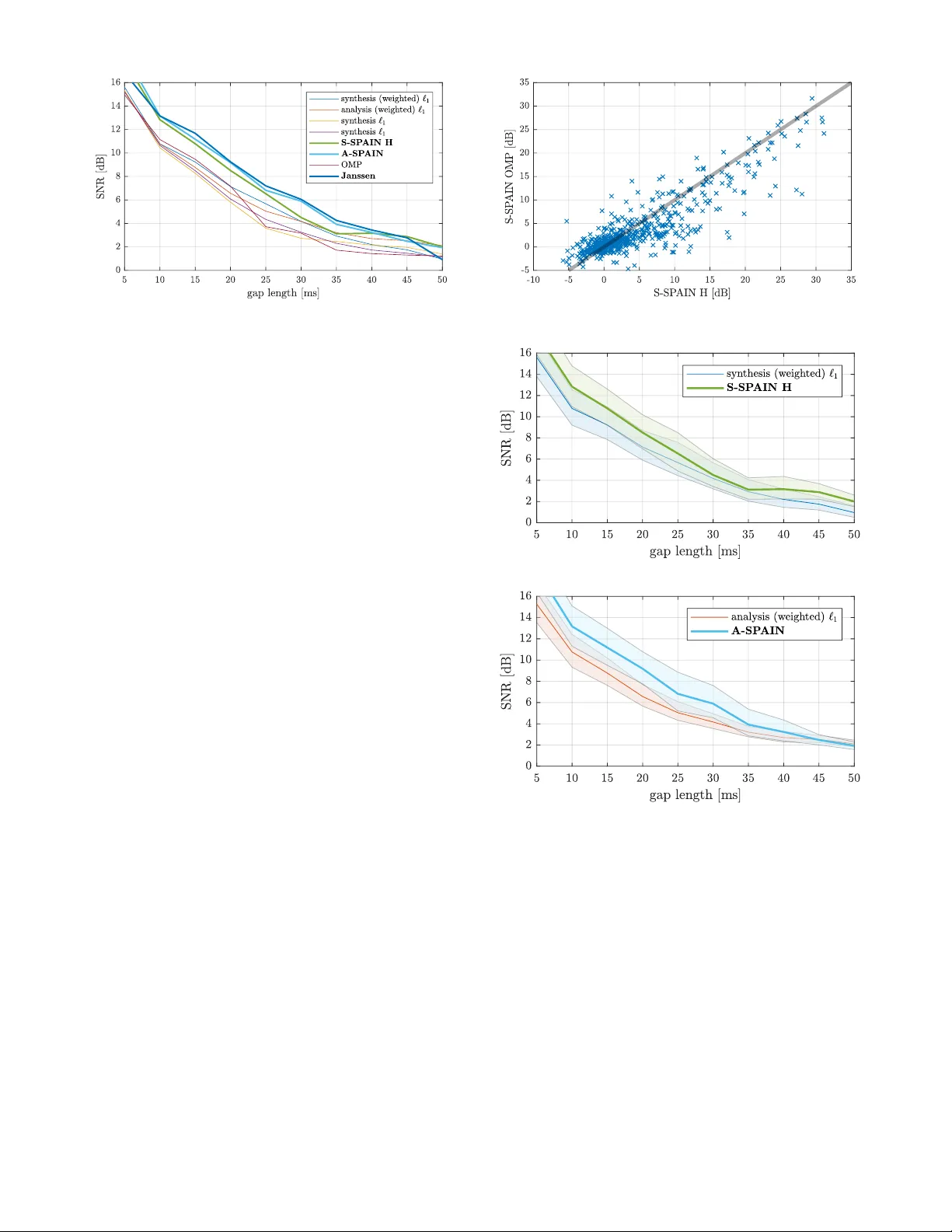
Introducing SP AIN (SP arse Audio INpainter) Ond ˇ rej Mokrý ?, † P avel Záviška ? P avel Rajmic ? Vít ˇ ezslav V eselý † ? Signal Processing Laboratory , Brno Univ ersity of T echnology , Brno, Czech Republic † Faculty of Mechanical Engineering, Brno Uni versity of T echnology , Brno, Czech Republic Email: {170583, xzavis01, rajmic, vitezsla v .vesely}@vutbr .cz Abstract —A novel sparsity-based algorithm for audio inpaint- ing is proposed. It is an adaptation of the SP ADE algorithm by Kiti ´ c et al., originally developed for audio declipping, to the task of audio inpainting. The new SP AIN (SParse A udio INpainter) comes in synthesis and analysis variants. Experiments show that both A-SP AIN and S-SP AIN outperform other sparsity-based inpainting algorithms. Moreov er , A-SP AIN performs on a par with the state-of-the-art method based on linear prediction in terms of the SNR, and, for lar ger gaps, SP AIN is ev en slightly better in terms of the PEMO-Q psychoacoustic criterion. Index T erms —Inpainting, Sparse, Cosparse, Synthesis, Analysis I . I N T RO D U C T I O N The term “inpainting” has spread to the audio processing community from the image processing field, when a paper by Adler et al. was published, entitled simply “ Audio inpainting” [1]. The goal of so termed restoration task is to fill degraded or missing parts of data, based on its reliable part, and preferably in an unobtrusi ve way . Although the term “inpainting” is rather new in this context, the problem itself is much older and different approaches hav e been proposed to deal with it in past decades. One of the first successful approaches was the time-domain interpolation of the missing audio samples. An adapti ve in- terpolation method was presented by Janssen et al. in [2], which was built on modeling the signal as an autoregressiv e (AR) process. The method can be roughly described as the minimization of a suitable functional, which includes as the variables both the estimates of the missing samples and the AR coefficients of the restored signal. Although the algorithm is designed as iterati ve, only a single iteration w as consid- ered in [2]. On today’ s hardware, nonetheless, hundreds of iterations can be computed in a reasonably short time. Doing this improves the results substantially and keeps the Janssen algorithm the state-of-the-art in audio inpainting in terms of the SNR. Note, howe ver , that when applied to compact gaps, the AR-modeling suggests that this method is successful for sounds that contain harmonics which do not e volve within the gap. As such, this approach is beneficial for gaps of up to ca 45 milliseconds, which can be observed also from the experiments described belo w . V arious prediction methods were also presented in [3]. The work was supported by the joint project of the FWF and the Czech Sci- ence Foundation (GA ˇ CR): numbers I 3067-N30 and 17-33798L, respectiv ely . Research described in this paper was financed by the National Sustainability Program under grant LO1401. Infrastructure of the SIX Center was used. A different approach is the sparsity-based audio inpainting, reported more recently in [1]. It benefits from the observation that the energy of an audio signal is often concentrated in a relatively small number of coefficients, with respect to a suitable, redundant time-frequency transform. The goal is to find a signal that has sparse representation under a transform such as the STFT (Short-Time Fourier T ransform, aka the Discrete Gabor Transform, DGT), while it belongs to the set of feasible solutions; for audio inpainting, a solution is feasible if it is identical to the reliable parts of the signal. The above requirements can be formulated as an optimiza- tion task. Its solution cannot be attained in practice due to the NP-hardness, but the solution can be reasonably approximated, for example using the Orthogonal Matching Pursuit (OMP) as in [1]. Another kind of approximation uses the ` 1 norm, which leads to a conv enient con vex minimization [4]. One of the modern approaches is also to search for sparsity in a non- local w ay [5], or using statistical prior information about the sparse representation [6]. Further methods hav e been developed to deal with long missing segments of audio signal. Stationary signals can be restored using sinusoidal modeling [7] or via model-based interpolation schemes [8]. In repetitiv e signals such as rock and pop music, there is usually an intact part sufficiently similar to the distorted part; this fact is utilized for filling the missing data in [9]. A dif ferent method, still based on self-similarity , was introduced in [10], aiming originally at the packet loss concealment. One of the latest methods employs a deep neural network for the task of audio inpainting [11]. The algorithm presented in the paper is inspired by the state-of-the-art among sparsity-based approaches to audio de- clipping, the so-called SParse Audio DEclipper (SP ADE) [12], [13] and it is in line with the universal framew ork presented in [14]. W e benefit from the close relation between the sparsity- based inpainting and declipping problems. W e formulate the two v ariants of the inpainting problem as the optimization tasks min x , z k z k 0 s. t. x ∈ Γ and k A x − z k 2 ≤ ε, (1a) min x , z k z k 0 s. t. x ∈ Γ and k x − D z k 2 ≤ ε, (1b) where (1a) and (1b) present the formulation referred to as the analysis and the synthesis v ariant, respectiv ely . In both formulations, Γ = Γ( y ) ⊂ C N is the set of feasible solutions (i.e. the set of time-domain signals that are equal to the observed signal y in its reliable parts), A : C N → C P is the analysis operator of a Parse v al tight frame and D = A ∗ is its synthesis counterpart, with P ≥ N [15]. The formulation (1) reflects the goal to find a signal from Γ with the highest- sparsity representation, as was informally stated abov e. The intention is to make use of the Alternating Direction Method of Multipliers (ADMM) for the optimization of the abov e non-con vex problems, as was the case in the original SP ADE paper [12]. For this purpose, a more appropriate formulation is needed. W e introduce the (unknown) sparsity k , which is to be minimized, and indicator functions 1 of two sets: the set of feasible solutions Γ and the set of k -sparse vectors, the latter denoted ` 0 ≤ k for short. This leads to min x , z ,k { ι Γ ( x ) + ι ` 0 ≤ k ( z ) } s.t. ( A x − z = 0 , x − D z = 0 . (2) Note that in (2), a more conservati ve constraint binding the variables x and z is used compared to (1). The reason is that such a constraint falls within the general ADMM scheme [17]. Such an alteration is ne vertheless legitimate, since in the resulting iterati ve algorithm presented below , the stopping criterion will in ef fect relax the constraint into the form of (1). I I . S P A I N ( S PA R S E A U D I O I N PA I N T E R ) In [12], the SP ADE algorithm was introduced to tackle (2). It is built on the idea that for a fixed k , problem (2) can be approximately solved by the ADMM. The SP ADE increases the value of k during the iterations of ADMM (starting from a sufficiently small value), until the condition k A x − z k 2 ≤ ε (analysis approach, A-SP ADE) or k x − D z k 2 ≤ ε (synthesis approach, S-SP ADE) is met for the chosen tolerance ε > 0 . This ensures k -sparsity of the signal coefficients during itera- tions and the algorithm thus provides an approximation of the solution to (1). Section II-A shows that A-SP AIN can be deri ved from A-SP ADE. In Subsection II-B, on the other hand, S-SP AIN is introduced as a brand ne w inpainting algorithm. The deriv ation is in line with the new variant of S-SP ADE for declipping, proposed in [18]. A. A-SP AIN derived fr om A-SP ADE The A-SP ADE algorithm (Alg. 1) was originally designed for the declipping task, where the set of feasible solutions Γ is the (conv ex) set of time-domain signals whose samples are identical to the observed ones in the reliable part, while the restored samples are required to lie abov e or below the upper or the lower clipping thresholds, respectiv ely; see [12] or [13] for more details. The key observ ation leading to SP AIN is that the for- mulations of inpainting and declipping differ only by the definition of the set of feasible solutions Γ , which is actually less restrictive for inpainting, since it does not in volve any requirements on the samples at unreliable positions. Alg. 1 is 1 The indicator function of a set Ω , denoted ι Ω ( x ) , attains the value 0 for x ∈ Ω and ∞ otherwise [16]. formulated general enough to cov er both the A-SP ADE and the new A-SP AIN. In effect, the actual task being solved is a matter of the projection on line 3 of the algorithm. The operator H k used in the algorithm denotes hard thresh- olding, which sets all but k largest elements of the argument to zero. Note that in our implementation, the structures of D and A and the fact that a real signal is being processed are taken into account, leading to thresholding complex-conjugate pairs of coefficients at a time instead of thresholding of a single vector element. Although the analysis version of the SP ADE algorithm was deriv ed from ADMM in [12] based on the formulation (2), the synthesis variant was surprisingly built on a dif ferent basis (see the technical report [19] for further explanation). A more consistent approach is to deri ve the synthesis variant in analogy to the analysis variant. Thus, in the follo wing subsection, the novel deriv ation of S-SP AIN from ADMM is briefly described. B. S-SP AIN derived fr om ADMM The ADMM is a scheme to solve optimization problems of the form min z f ( z ) + g ( D z ) , (3) where D is a linear operator . The functions f , g are assumed to be real and conv ex. Problem (3) can be reformulated by introducing a slack variable x such that x = D z , leading to min z , x f ( z ) + g ( x ) s.t. x − D z = 0 , (4) which corresponds to the synthesis variant of (2). Next, the Augmented Lagrangian is formed as L ρ ( x , z , λ ) = f ( x ) + g ( z ) + λ > ( x − D z ) + ρ 2 k x − D z k 2 2 , (5) where ρ > 0 is called the penalty parameter and λ ∈ R N is the dual v ariable. The general scheme of ADMM then consists of three steps—minimization of L ρ ov er z , minimization of L ρ ov er x and the update of the dual variable λ . For the purpose of audio inpainting, we set f ( z ) = ι ` 0 ≤ k ( z ) and g ( x ) = ι Γ ( x ) . Note that such a function f is not conv ex, therefore the conditions of ADMM are not met. Ne vertheless, ADMM may con verge e ven in such a case and the e xperiments show that it provides reasonable results for audio inpainting. It is conv enient to introduce the so-called scaled dual v ari- able u = λ /ρ at this moment. After this, it is straightforward to arriv e at the ADMM steps for S-SP AIN in the follo wing form: z ( i +1) = arg min z k D z − x ( i ) + u ( i ) k 2 2 s.t. k z k 0 ≤ k , (6a) x ( i +1) = arg min x k D z ( i +1) − x + u ( i ) k 2 2 s.t. x ∈ Γ , (6b) u ( i +1) = u ( i ) + D z ( i +1) − x ( i +1) . (6c) In the con ve x case, the minimizations over x and over z can be switched without affecting the conv ergence of ADMM [17]. W e assume that the con vergence will not be violated in the non-con vex case either . Algorithm 1: A-SP ADE / A-SP AIN, depending on the particular choice of Γ Require: A, y , Γ , s, r , ε 1 ˆ x (0) = y , u (0) = 0 , i = 0 , k = s 2 ¯ z ( i +1) = H k  A ˆ x ( i ) + u ( i )  3 ˆ x ( i +1) = arg min x k A x − ¯ z ( i +1) + u ( i ) k 2 2 s.t. x ∈ Γ 4 if k A ˆ x ( i +1) − ¯ z ( i +1) k 2 ≤ ε then 5 terminate 6 else 7 u ( i +1) = u ( i ) + A ˆ x ( i +1) − ¯ z ( i +1) 8 i ← i + 1 9 if i mod r = 0 then 10 k ← k + s 11 end 12 go to 2 13 end 14 retur n ˆ x = ˆ x ( i +1) The solution to the subproblem (6b) is the projection of ( D z ( i +1) + u ( i ) ) onto Γ , which is easy to compute in the time domain. The subproblem (6a) is more challenging—it corresponds to the sparse synthesis approximation, where the goal is to get as close as possible to the signal ( x ( i ) − u ( i ) ) by synthesis using D in such a way that the e xpansion coefficients are k -sparse. Such a problem is NP-hard due to the non- orthogonality of D in practice; therefore approximate solutions are enforced. One possibility is to utilize hard thresholding and compute z ( i +1) ≈ H k  D ∗ ( x ( i ) − u ( i ) )  . (7) In [19] we show that such an approximation is reasonably close to the solution of (6a). Note that in A-SP AIN, on the contrary , the thresholding step provides an exact solution of the corresponding ADMM subproblem. Alternativ ely , z ( i +1) can be approximated using k iterations of OMP [20], which was not considered neither in the original SP ADE [12] nor the nov el synthesis version [18]. Such an approach is, howe ver , computationally much more demanding than the thresholding (since each iteration of OMP employs one synthesis and one analysis) and the e xperiments sho w that although it pro vides a better approximation for the solution of (6a), it surprisingly does not lead to a better result of the whole S-SP AIN algo- rithm. The S-SP AIN algorithm is presented in Alg. 2. In the fol- lowing section, the S-SP AIN variants using hard thresholding and OMP as an approximation of step 2 of the algorithm will be denoted as S-SP AIN H and S-SP AIN OMP, respectiv ely . I I I . E X P E R I M E N T S A N D R E S U LT S A. Evaluation based on signal-to-noise ratio (SNR) For the experiment, ten music recordings sampled at 16 kHz or 44.1 kHz were used, co vering different degrees of sparsity of the STFT coefficients. The main source was the signals that were examined in the papers [1], [12], [21]. Algorithm 2: S-SP AIN, task in step 2 is to be approxi- mated either by the hard thresholding or OMP Require: D , y , Γ , s, r , ε 1 ˆ x (0) = D ∗ y , u (0) = 0 , i = 0 , k = s 2 ¯ z ( i +1) = arg min z k D z − ˆ x ( i ) + u ( i ) k 2 2 s.t. k z k 0 ≤ k 3 ˆ x ( i +1) = arg min x k D ¯ z ( i +1) − x + u ( i ) k 2 2 s.t. x ∈ Γ 4 if k D ¯ z ( i +1) − ˆ x ( i +1) k 2 ≤ ε then 5 terminate 6 else 7 u ( i +1) = u ( i ) + D ¯ z ( i +1) − ˆ x ( i +1) 8 i ← i + 1 9 if i mod r = 0 then 10 k ← k + s 11 end 12 go to 2 13 end 14 retur n ˆ x = ˆ x ( i +1) In each test instance, the objecti ve was to recover a signal containing six g aps, starting at random points in the signal such that the gaps do not ov erlap and are not too close to affect the restoration [22]. The gap length was chosen from the set of 10 a vailable lengths, distributed between 5 and 50 ms. As the competitors of SP AIN, we used the Janssen al- gorithm, the OMP and both the synthesis and the analysis approaches of the ` 1 relaxation. 2 In OMP and SP AIN, we used the ov ercomplete DFT with redundancy of the transform set to 2 (meaning that the number of frequency channels is twice the number of signal samples). All algorithms were applied frame-wise: the signal was windowed using the Hann window 64 ms long with a shift of 16 ms (i.e. 75% ov erlap), and the restored blocks were combined using the overlap-add scheme. F or the ` 1 relaxation, the DGT was used with the same window parameters and with number of frequency channels corresponding to length of the transform window in samples. Besides this, weighted ` 1 relaxation was also employed. 3 As the performance measure, we used the signal-to-noise ratio (SNR), defined SNR ( x , ˆ x ) = 10 log 10 k x k 2 2 k x − ˆ x k 2 2 [dB] , (8) where ˆ x stands for the recov ered gap and x denotes the corresponding segment of the uncorrupted signal [1]. Fig. 1 shows the overall results; for each gap length and each algorithm, the average value of SNR was computed from all the signals and all positions of the gap. It is clear that for 2 Implementation of the Janssen algorithm was taken from the Audio In- painting T oolbox [1]. OMP was implemented using the Sparsify T oolbox [23]. For the synthesis and the analysis ` 1 relaxations, our own implementations of the Douglas-Rachford and the Chambolle-Pock algorithms were used, respectiv ely . 3 In weighted ` 1 relaxation, the objective function is k W · k 1 . The diagonal matrix W allows us to fav or chosen coefficients of the STFT when searching for the restored signal. The same weighting, i.e. according to ` 2 norm of truncated atoms, was proposed in [1] for OMP . Fig. 1: Inpainting results in terms of the SNR. gaps of up to 40 ms, Janssen and A-SP AIN outperform all other methods and that these two algorithms behave almost identically in terms of the SNR (the biggest difference is for the longest gaps greater than 45 ms, where the performance of Janssen drops). Regarding S-SP AIN, the performance is comparable with A-SP AIN and Janssen for shorter gaps (up to 25 ms), and it outperforms the OMP and the ` 1 -relaxation methods e ven for the longer gaps. A possible e xplanation of the superiority of A-SP AIN ov er S-SP AIN is that the ADMM subproblems in the analysis v ariant are solved exactly , whereas in the synthesis one, the thresholding operator provides just an approximation of (6a). Note that in Fig. 1, results of S-SP AIN OMP are not presented. The reason is the compu- tational complexity of this approach (a single test instance takes up to a few days!). The scatter plot in Fig. 2 sho ws detailed comparison of S-SP AIN H with S-SP AIN OMP. Due to the computational time consumed by the S-SP AIN OMP, a shortened exper- iment was performed with both the gap lengths and the window length shortened to their quarter compared to the first experiment (i.e. windo w length 16 ms, overlap 4 ms, gap lengths ranging from 1.25 to 12.5 ms). Each cross in Fig. 2 corresponds to one test instance and its coordinates are SNR for S-SP AIN H and S-SP AIN OMP. The diagonal line in the plot divides the areas in which S-SP AIN H (under the line) or S-SP AIN OMP (abov e the line) perform better . It is clear that except for a small area corresponding to a very low SNR, S-SP AIN H outperforms S-SP AIN OMP in majority (approx. 58 %) of cases. Also the single-tailed Wilcoxon signed rank test 4 suggests that the median of results of S-SP AIN H is greater than in case of S-SP AIN OMP with significance lev el 0.05. This result is quite surprising since the OMP is supposed to solve the optimization subproblem (6a) better than the simpler hard thresholding does. For a more thorough analysis of the results, Fig. 3 provides comparison of S-SP AIN H and A-SP AIN with corresponding con vex approaches, sho wing the bootstrap 95% confidence intervals [24] for the mean value of SNR. It can be seen from the width of the confidence intervals that the comparison with 4 Performed using function signrank in MA TLAB. Fig. 2: Comparison of S-SP AIN H and S-SP AIN OMP. (a) synthesis model (b) analysis model Fig. 3: Bootstrap 95% confidence intervals for the mean value of SNR for chosen curv es from Fig. 1. The estimates with significance lev el 0.05 was computed using bootstrapping [24] with 10 000 random draws from the population for each combination of algorithm and gap length. Janssen w ould not be statistically significant, while, on the other hand, SP AIN clearly outperforms the ` 1 methods in most cases. B. Evaluation based on PEMO-Q For further comparison of SP AIN with Janssen, we per- formed a second experiment, aiming at a more profound ev al- uation using PEMO-Q [25]. In order to correctly ev aluate the restored signals with PEMO-Q, only sound excerpts sampled (a) gap length 20 ms (b) gap length 30 ms (c) gap length 40 ms (d) gap length 50 ms Fig. 4: A verage ODG values. Showing results for the ob- served, degraded signal (anchor , An) and the reconstruction by A-SP AIN (A), S-SP AIN H (S) and Janssen (J). at 44.1 kHz from the pre vious e xperiment had to be used (which makes six test signals in total). W e also considered only the gaps with lengths from the set of { 20 , 30 , 40 , 50 } ms. The measured quantity w as the objective differ ence grade (ODG) which simulates the human perception, comparing the restored signal to the reference (original, not degraded signal). The ODG ranges from 0 to − 4 and rates the audio degradation as: 0 . 0 Imperceptible − 1 . 0 Perceptible, but not annoying − 2 . 0 Slightly annoying − 3 . 0 Annoying − 4 . 0 V ery annoying The results in terms of ODG are presented in Fig. 4. Each plot sho ws av erage v alues o ver the six audio samples, given the gap length. As expected, the plots indicate that the longer the gap, the worse the reconstruction. Nevertheless, the remarkable result here is that besides the gap length of 20 ms, A-SP AIN slightly outperforms both S-SP AIN H and Janssen. I V . S O F T W A R E A N D DAT A The MA TLAB codes for SP AIN and the sound excerpts are av ailable at https://bit.ly/2zdhbpp. V . C O N C L U S I O N The paper presented a novel inpainting algorithm (SP AIN) dev eloped by an adaptation of successful declipping method, SP ADE, to the context of inpainting. It was shown that the analysis variant of SP AIN performs the best in terms of SNR among sparsity-based methods. Furthermore, A-SP AIN was demonstrated to reach results on a par with the state-of-the- art Janssen algorithm for audio inpainting in terms of SNR. Finally , the objecti ve test using PEMO-Q, which takes into account the human perception of sound, showed that A-SP AIN ev en slightly outperforms Janssen for larger gap sizes. R E F E R E N C E S [1] A. Adler, V . Emiya, M. Jafari, M. Elad, R. Gribon val, and M. Plumbley , “ Audio Inpainting, ” IEEE Tr ansactions on Audio, Speech, and Language Pr ocessing , vol. 20, no. 3, pp. 922–932, 2012. [2] A. J. E. M. Janssen, R. N. J. V eldhuis, and L. B. Vries, “ Adaptive interpolation of discrete-time signals that can be modeled as autoregres- siv e processes, ” IEEE Trans. Acoustics, Speech and Signal Pr ocessing , vol. 34, no. 2, pp. 317–330, 1986. [3] M. Fink, M. Holters, and U. Zölzer, “Comparison of various predictors for audio extrapolation, ” in Proc. of the 16th Int. Conference on Digital Audio Effects (D AFx-13) , Maynooth, 2013, pp. 1–7. [4] F . Lieb and H.-G. Stark, “ Audio inpainting: Ev aluation of time-frequency representations and structured sparsity approaches, ” Signal Pr ocessing , vol. 153, pp. 291–299, 2018. [5] I. T oumi and V . Emiya, “Sparse non-local similarity modeling for audio inpainting, ” in 2018 ICASSP . IEEE, 2018. [6] A. Adler, “Covariance-assisted matching pursuit, ” IEEE Signal Process- ing Letters , vol. 23, no. 1, pp. 149–153, 2016. [7] M. Lagrange, S. Marchand, and J.-B. Rault, “Long interpolation of audio signals using linear prediction in sinusoidal modeling, ” J. Audio Eng. Soc , vol. 53, no. 10, pp. 891–905, 2005. [8] P . A. A. Esquef, V . Välimäki, K. Roth, and I. Kauppinen, “Interpolation of long gaps in audio signals using the warped Burg’ s method, ” in Pr oceedings of the 6th Int. Conference on Digital Audio Effects (DAFx- 03), 2003. [9] N. Perraudin, N. Holighaus, P . Majdak, and P . Balazs, “Inpainting of long audio segments with similarity graphs, ” IEEE/ACM T ransactions on Audio, Speech, and Language Pr ocessing , pp. 1–1, 2018. [10] Y . Bahat, Y . Y . Schechner, and M. Elad, “Self-content-based audio inpainting, ” Signal Pr ocessing , vol. 111, no. 0, pp. 61–72, 2015. [11] A. Marafioti, N. Perraudin, N. Holighaus, and P . Majdak, “ A context encoder for audio inpainting, ” 2018. [Online]. A vailable: https: //arxiv .org/pdf/1810.12138.pdf [12] S. Kiti ´ c, N. Bertin, and R. Gribon val, “Sparsity and cosparsity for audio declipping: A flexible non-conv ex approach, ” in L V A/ICA 2015 , Liberec, 2015. [13] P . Záviška, P . Rajmic, Z. Pr ˚ uša, and V . V eselý, “Revisiting synthesis model in sparse audio declipper, ” in Latent V ariable Analysis and Signal Separation . Cham: Springer International Publishing, 2018, pp. 429– 445. [14] C. Gaultier , N. Bertin, S. Kiti ´ c, and R. Gribonv al, “ A modeling and algorithmic framew ork for (non)social (co)sparse audio restoration, ” 2017. [Online]. A vailable: https://arxiv .org/abs/1711.11259 [15] O. Christensen, F rames and Bases, An Introductory Course , Birkhäuser: Boston, 2008. [16] P . Combettes and J. Pesquet, “Proximal splitting methods in signal processing, ” F ixed-P oint Algorithms for Inverse Pr oblems in Science and Engineering , pp. 185–212, 2011. [17] S. P . Boyd, N. Parikh, E. Chu, B. Peleato, and J. Eckstein, “Distributed optimization and statistical learning via the alternating direction method of multipliers. ” F oundations and T r ends in Machine Learning , vol. 3, no. 1, pp. 1–122, 2011. [18] P . Záviška, P . Rajmic, O. Mokrý, and Z. Pr ˚ uša, “ A proper version of synthesis-based sparse audio declipper, ” in 2019 ICASSP , Brighton, 2019, pp. 591–595. [19] P . Záviška, O. Mokrý, and P . Rajmic, “S-SP ADE done right: Detailed study of the Sparse Audio Declipper algorithms, ” Brno Univ ersity of T echnology , techreport, 2018. [Online]. A vailable: https://arxiv .org/pdf/1809.09847.pdf [20] M. Elad, Sparse and redundant r epresentations: F rom theory to appli- cations in signal and image pr ocessing . Springer , 2010. [21] K. Siedenburg and M. Dörfler, “Structured sparsity for audio signals, ” in D AFx-11 , 2011, pp. 23–26. [22] P . Rajmic, H. Bartlo vá, Z. Pr ˚ uša, and N. Holighaus, “ Acceleration of audio inpainting by support restriction, ” in 2015 ICUMT , 2015. [23] T . Blumensath, “Sparsify toolbox”. [Online]. A vailable: https://www . southampton.ac.uk/engineering/about/staff/tb1m08.page#softw are [24] B. Efron and R. J. Tibshirani, An introduction to the bootstrap . New Y ork: Chapmann & Hall, 1994. [25] R. Huber and B. K ollmeier, “PEMO-Q—A new method for objectiv e audio quality assessment using a model of auditory perception, ” IEEE T rans. Audio Speech Language Proc. , vol. 14, no. 6, pp. 1902–1911, 2006.