Poly-time universality and limitations of deep learning

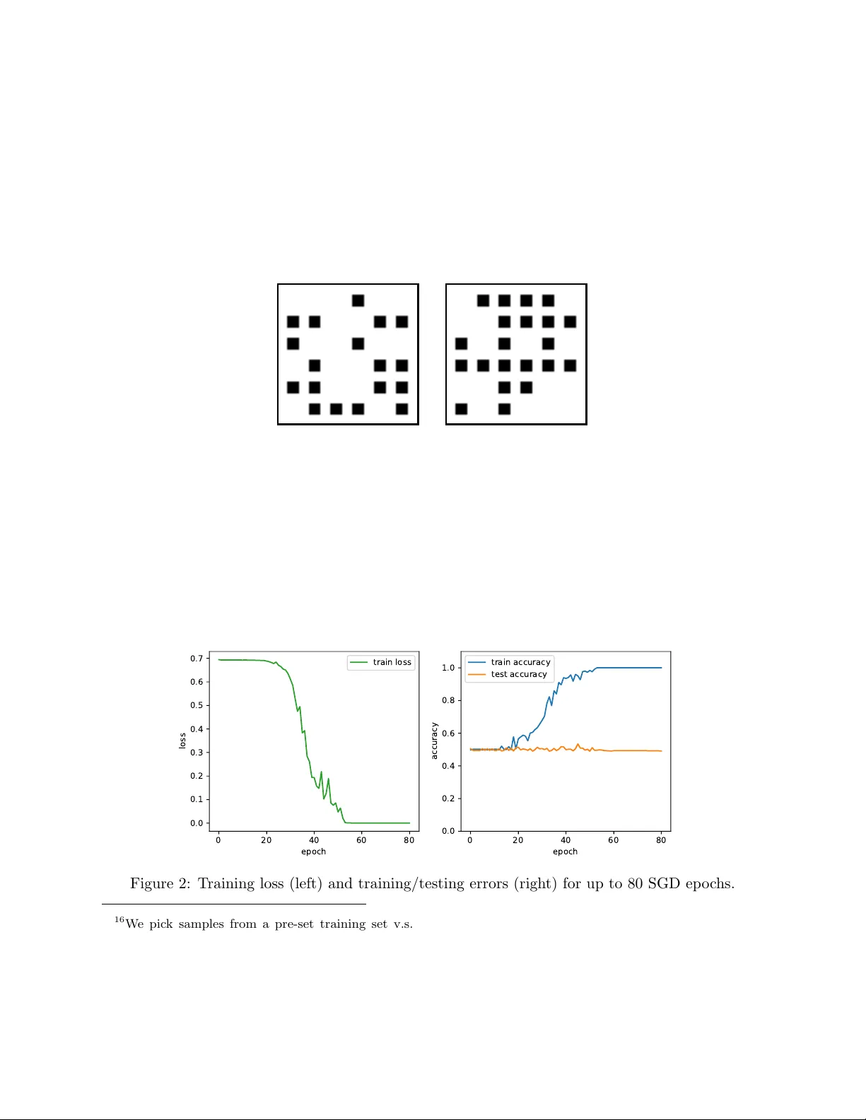
P oly-time univ ersalit y and limitations of deep learning Emman uel Abb e EPFL Colin Sandon MIT Abstract The goal of this pap er is to c haracterize function distributions that deep learning can or cannot learn in p oly-time. A univ ersality result is pro ved for SGD-based deep learning and a non-univ ersality result is pro v ed for GD-based deep learning; this also giv es a separation b et ween SGD-based deep learning and statistical query algorithms: (1) De ep le arning with SGD is efficiently universal. Any function distribution that can be learned from samples in p oly-time can also b e learned by a p oly-size neural net trained with SGD on a p oly-time initialization with p oly-steps, p oly-rate and p ossibly p oly-noise. Therefore deep learning provides a univ ersal learning paradigm: it was known that the appro ximation and estimation errors could b e controlled with p oly-size neural nets, using ERM that is NP-hard; this new result sho ws that the optimization error can also b e controlled with SGD in p oly-time. The picture changes for GD with large enough batches: (2) R esult (1) do es not hold for GD: Neural nets of poly-size trained with GD (full gradients or large enough batches) on an y initialization with p oly-steps, p oly-range and at least poly-noise cannot learn any function distribution that has sup er-p olynomial cr oss-pr e dictability, where the cross-predictabilit y gives a measure of “av erage” function correlation – relations and distinctions to the statistical dimension are discussed. In particular, GD with these constraints can learn efficien tly monomials of degree k if and only if k is constan t. Th us (1) and (2) p oint to an interesting contrast: SGD is universal even with some p oly-noise while full GD or SQ algorithms are not (e.g., parities). This thus gives a separation b etw een SGD-based deep learning and SQ algorithms. Finally , w e complete these by sho wing that the cross-predictabilit y also imp edes SGD once larger amounts of noise are added on the initialization and gradients, or when sufficiently few weigh t are up dating p er time step (as in co ordinate descen t). 1 Con ten ts 1 In tro duction 3 1.1 Con text and this paper . . . . . . . . . . . . . . . . . . . . . . . . . . . . . . . . . . 3 1.2 Problem form ulations and learning ob jectiv es . . . . . . . . . . . . . . . . . . . . . . 4 1.3 Informal results: Cross-predictabilit y , junk-flow and universalit y . . . . . . . . . . . 6 2 Results 8 2.1 Definitions and models . . . . . . . . . . . . . . . . . . . . . . . . . . . . . . . . . . . 8 2.2 P ositive results . . . . . . . . . . . . . . . . . . . . . . . . . . . . . . . . . . . . . . . 9 2.3 Negativ e results . . . . . . . . . . . . . . . . . . . . . . . . . . . . . . . . . . . . . . . 10 2.3.1 GD with noise . . . . . . . . . . . . . . . . . . . . . . . . . . . . . . . . . . . 10 2.3.2 SGD with memory constraint . . . . . . . . . . . . . . . . . . . . . . . . . . . 12 2.3.3 SGD with additional randomness . . . . . . . . . . . . . . . . . . . . . . . . . 13 2.4 Pro of tec hniques: undistinguishabilit y , em ulation and sequen tial learning algorithms 14 3 Related literature 16 3.1 Minsky and P ap ert . . . . . . . . . . . . . . . . . . . . . . . . . . . . . . . . . . . . . 16 3.2 Statistical querry algorithms . . . . . . . . . . . . . . . . . . . . . . . . . . . . . . . . 17 3.3 Memory-sample trade-offs . . . . . . . . . . . . . . . . . . . . . . . . . . . . . . . . . 18 3.4 Gradien t concen tration . . . . . . . . . . . . . . . . . . . . . . . . . . . . . . . . . . . 19 4 Some challenging functions 20 4.1 P arities . . . . . . . . . . . . . . . . . . . . . . . . . . . . . . . . . . . . . . . . . . . 20 4.2 Comm unity detection and connectivit y . . . . . . . . . . . . . . . . . . . . . . . . . . 22 4.3 Arithmetic learning . . . . . . . . . . . . . . . . . . . . . . . . . . . . . . . . . . . . . 22 4.4 Bey ond lo w cross-predictability . . . . . . . . . . . . . . . . . . . . . . . . . . . . . . 23 5 Pro ofs of negativ e results 25 5.1 Pro of of Theorem 3 . . . . . . . . . . . . . . . . . . . . . . . . . . . . . . . . . . . . . 25 5.1.1 Pro of of Theorem 4 . . . . . . . . . . . . . . . . . . . . . . . . . . . . . . . . 28 5.2 Pro of of Theorem 5 . . . . . . . . . . . . . . . . . . . . . . . . . . . . . . . . . . . . . 29 5.2.1 Learning from a bit . . . . . . . . . . . . . . . . . . . . . . . . . . . . . . . . 29 5.2.2 Distinguishing with SLAs . . . . . . . . . . . . . . . . . . . . . . . . . . . . . 32 5.2.3 Application to SGD . . . . . . . . . . . . . . . . . . . . . . . . . . . . . . . . 37 5.3 Pro of of Theorem 6 . . . . . . . . . . . . . . . . . . . . . . . . . . . . . . . . . . . . . 38 5.3.1 Uniform noise and SLAs . . . . . . . . . . . . . . . . . . . . . . . . . . . . . . 39 5.3.2 Gaussian noise, noise accumulation, and blurring . . . . . . . . . . . . . . . . 40 5.3.3 Means, SLAs, and Gaussian distributions . . . . . . . . . . . . . . . . . . . . 45 6 Pro ofs of p ositiv e results: univ ersality of deep learning 51 6.1 Em ulation of arbitrary algorithms . . . . . . . . . . . . . . . . . . . . . . . . . . . . 52 6.2 Noisy em ulation of arbitrary algorithms . . . . . . . . . . . . . . . . . . . . . . . . . 62 6.3 Additional commen ts on the emulation . . . . . . . . . . . . . . . . . . . . . . . . . . 70 2 1 In tro duction 1.1 Con text and this pap er It is kno wn that the class of neural netw orks (NNs) with p olynomial netw ork size can express an y function that can b e implemented in a giv en p olynomial time [ P ar94 , Sip06 ], and that their sample complexit y scales p olynomially with the netw ork size [ AB09 ]. Th us NNs hav e fav orable appro ximation and estimation errors. The main challenge is with the optimization error, as there is no kno wn efficien t training algorithm for NNs with pro v able guaran tees, in particular, it is NP-hard to implemen t the ERM rule [ KS09 , DSS16 ]. The success behind deep learning is to train de ep NNs with stochastic gradien t descent or the lik e; this giv es record p erformances 1 in image [ KSH12 ], sp eech [ HD Y + 12 ], document recognitions [ LBBH98 ] and increasingly more applications [ LBH15 , GBC16 ]. This raises the question of whether SGD complements neural net works to a univ ersal learning paradigm [ SSBD14 ], i.e., capable of learning efficiently any efficiently learnable function distribution. (i) This pap er answ ers this question in the affirmative. It is sho wn that training poly-size neural nets with SGD in poly-steps allows one to learn any function distribution that is learnable by some algorithm running in p oly-time with p oly-man y samples. This part is resolved using a sp ecific non-random net initialization that is implemented in p oly-time and not dependent on the function to be learned, and that allows to emulate any efficien t learning algorithm under SGD training. (ii) W e further sho w that this p ositiv e result is ac hieved with some robustness to noise: p olynomial noise can b e added to the gradients and w eights can b e of polynomial precision and the result still holds. Therefore, in a computational theoretic sense, deep learning giv es a univ ersal learning framew ork. (iii) This p ositive result is also put in contrast with the following one: the same univ ersality result do es not hold when using full gradien t descen t or large enough batches 2 , due to the existence of efficien tly learnable function distribution ha ving lo w cross-predictabilit y (see definitions b elow). This also creates a separation betw een deep learning and statistical query (SQ) algorithms, whic h cannot afford suc h noise-robustness on function classes having high statistical (see more b elow). In a practical setting, there may b e no obvious reason to use the SGD replacemen t to a general learning algorithm, but this universalit y result sho ws that negativ e results about deep learning cannot be obtained without further constraints. T o obtain negative results ab out GD, we sho w that GD cannot learn in p oly-steps and with p oly-noise certain function distributions that hav e a low cross-predictability (a measure of a verage function correlation defined in Section 1.3 ). This is similar to the type of negativ e results that SQ algorithms pro vide, except for the differences that our results apply to statistical noise, to a w eaker learning requiremen t that focuses on an av erage-case rather than worst-case guarantee on the function class, and to p ossibly non-statistical queries as in SGD (with an accoun t giv en on the batc h size dep endencies). W e refer to Section 3.2 for further discussions on SQ algorithms and statistical dimension, as w ell as to [ Boi19 ] for further comparisons. Note that the dependency on the batc h size is particularly imp ortan t: with batch-size 1, w e sho w that SGD is univ ersal, and this breaks do wn as the batch size gets p olynomial. Therefore, while SGD can be view ed as a surrogate to GD that is computationally less expensive (but less effective in con vex settings), SGD turns out to b e universal while GD is not. Note the 1 While deep learning op erates in an ov erparametrized regime, and while SGD optimizes a highly non-con vex ob jective function, the training by SGD giv es astonishingly low generalization errors for these types of signals. 2 Some of the negative results presen ted here app eared in a preliminary version of the pap er [ AS18 ]; a few changes are obtained in the current version, with in particular the dep endency in the batch size for the negative result on GD. This allows to show that as the GD queries b ecome more random (smaller batches), the negative result breaks down. 3 sto c hasticity of SGD has already been advocated in differen t contexts, such as stabilit y , implicit regularization or to av oid bad critical points [ HRS16 , ZBH + 16 , PP17 , KL Y18 ]. As men tioned earlier, the amount of noise under whic h SGD can still learn in our p ositiv e result is large enough to break down not only GD, but more generally SQ algorithms. F or example, our p ositiv e result sho ws that SGD can learn efficiently parities with some p oly-noise, while GD or SQ algorithms break do wn in suc h cases. Note that parities w ere also kno wn to b e hard as far back as Minsky and P ap ert for the perceptron [ MP87 ], and our positive result requires indeed more than a single hidden la yer to succeed. Th us deep nets trained with SGD can b e more p o werful for generalization than deep nets trained with GD or than SQ algorithms. T o complement the story , w e also obtain negative results ab out SGD under low cross-predictabilit y if additional constraints are added on the num b er of weigh ts that can b e updated p er time steps (as in coordinate descent), or when larger amoun ts of noise are added on the initialization and on the gradien ts. Informal results are discussed in Section 1.3 and formal definitions and results are given in Section 2 . 1.2 Problem form ulations and learning ob jectiv es W e fo cus on Boolean functions to simplify the setting. Since it is known that any Boolean function that can be computed in time O ( T ( n )) can also be expressed b y a neural net work of size O ( T ( n ) 2 ) [ P ar94 , Sip06 ], it is not meaningful to ask whether an y suc h function f 0 can b e learned with a p oly-size NN and a descent algorithm that has degree of freedom on the initialization and knowledge of f 0 ; one can simply pre-set the net to express f 0 . Tw o more meaningful questions that one can ask are: 1. Can one learn a giv en function with an agnostic/random 3 initialization? 2. Can one learn an unknown function from a class or distribution with some choice of the initialization? F or the second question, one is not giv e a specific function f 0 but a class of functions, or more generally , a distribution on functions. W e fo cus here mainly on question 2, which gives a more general framew ork than restricting the initialization to b e random. Moreov er, in the case of symmetric function distributions, suc h as the parities discussed below, failure at 2 implies failure at 1. Namely , if we cannot learn a parit y function for a random selection of the supp ort S (see definitions below), w e cannot learn any given parit y function on a typical supp ort S 0 with a random initialization of the net, b ecause the latter is symmetrical. Nonetheless, question 1 may also b e in teresting for applications, as random (or random-lik e) initializations ma y b e used in practice. W e discuss in Section 1.3 how w e exp ect that our results and the notion of cross-predictabilit y exp ort to the setting of question 1. W e th us ha ve the following setting: • Let D = { +1 , − 1 } and X = D n b e the data domain and let Y = { +1 , − 1 } b e the lab el domain. W e w ork with binary v ectors and binary lab els for conv enience (sev eral of the results extend b ey ond this setting with appropriate reformulation of definitions). 3 A random initialization means i.i.d. w eights as discussed in Section 1.3 . 4 • Let P X b e a probabilit y distribution on the data domain X and P F b e a probabilit y distribution on Y X (the set of functions from X to Y ). W e also assume for conv enience that these distributions lead to balanced classes, i.e., that P ( F ( X ) = 1) = 1 / 2 + o n (1) when ( X , F ) ∼ P X × P F (non-balanced cases require adjustments of the definitions). • Our goal is to learn a function F dra wn under P F b y observing lab elled examples ( X , Y ) with X ∼ P X , Y = F ( X ). • In order to learn F w e can train our algorithm on lab elled examples with a descen t algorithm starting with an initialization f (0) and running for a n umber of steps T = T ( n ) (other parameters of the algorithm suc h as the learning rate are also sp ecified). In the case of GD, eac h step accesses the full distribution of lab elled examples, while for SGD, it only accesses a single labelled example p er step (see definitions b elo w). In all cases, after the training with ( f (0) , T ), the algorithm pro duces an estimator ˆ F f (0) ,T of F . In order to study negativ e results, w e will set what is arguably the least demanding learning requirement: w e say that ‘t ypical-weak learning’ is solv able in T time steps for the considered ( P X , P F ), if a net with initialization f (0) can be constructed suc h that: T ypic al-we ak le arning: P ( ˆ F f (0) ,S ( X ) = F ( X )) = 1 / 2 + Ω n (1) , (1) where the ab ov e probabilit y is o ver ( X , F ) ∼ ( P X × P F ) and any randomness p otentially used b y the algorithm. In other words, after training the algorithm on some initialization, w e can predict the lab el of a new fresh sample from P X with accuracy strictly b etter than random guessing, and this takes place when the unkno wn function is drawn under P F . F ailing at typical-w eak learning implies failing at most other learning requirements. F or example, failing at typical w eak learning for a uniform distribution on a certain class of functions implies failing at P AC learning that class of functions. How ever, for our p ositiv e results with SGD, we will not only show that one can typically weakly learn efficiently any function distribution that is t ypically w eakly learnable, but that we can in fact reproduce whatever accuracy an algorithm can ac hieve for the considered distribution. T o b e complete w e need to define accuracy and typical weak learning for m ore general algorithms: Definition 1. L et n > 0 , P X b e a pr ob ability distribution on X = D n for some set D , and P F b e a pr ob ability distribution on the set of functions fr om X to { +1 , − 1 } . Assume that these distributions le ad to b alanc e d classes, i.e., P ( F ( X ) = 1) = 1 / 2 + o n (1) when ( X , F ) ∼ P X × P F . Consider an algorithm A that, given ac c ess to an or acle that uses P X and F ∼ P F (e.g., samples under P X lab el le d by F ), outputs a function ˆ F . Then A le arns ( P F , P X ) with ac cur acy α if P { ˆ F ( X ) = F ( X ) } ≥ α , wher e the pr evious pr ob ability is taken over ( X , F ) ∼ P X × P F and any r andomness p otential ly use d by ˆ F . In p articular, we say that A (typic al ly-we akly) le arns ( P F , P X ) if it le arns ( P F , P X ) with ac cur acy 1 / 2 + Ω n (1) . F rom no w on w e often shorten ‘t ypical-w eak learning’ to simply ‘learning’. W e also talk ab out learning a ‘function distribution’ or a ‘distribution’ when referring to learning a pair ( P X , P F ). Example. The problem of learning parities corresponds normally to P X b eing uniform on { +1 , − 1 } n and P F b eing uniform on the set of parity functions defined b y P = { p s : s ⊆ [ n ] } , where p s : { +1 , − 1 } n → { +1 , − 1 } is suc h that p s ( x ) = Q i ∈ s x i . So nature pic ks S uniformly at random in 2 [ n ] , and with kno wledge of P but not S , the problem is to learn whic h set S w as pic ked from samples ( X, p S ( X )). 5 1.3 Informal results: Cross-predictabilit y , junk-flow and univ ersality Definition 2. F or a p ositive inte ger m , a pr ob ability me asur e P X on the data domain X , and a pr ob ability me asur e P F on the class of functions F fr om X to Y = { +1 , − 1 } , we define the cr oss-pr e dictability by CP m ( P X , P F ) := E ( X m ,F,F 0 ) ∼ P m X × P F × P F ( E X ∼ P X m F ( X ) F 0 ( X )) 2 , (2) wher e X m = ( X 1 , . . . , X m ) has i.i.d. c omp onents under P X , F , F 0 ar e indep endent of X m and i.i.d. under P F , and X is dr awn indep endently of ( F , F 0 ) under the empiric al me asur e of X m , i.e., P X m = 1 m P m i =1 δ X i . Note the follo wing equiv alent representations: CP m ( P X , P F ) = 1 m +  1 − 1 m  CP ∞ ( P X , P F ) , (3) where CP ∞ ( P X , P F ) := E F,F 0 ∼ P F ( E X ∼ P X F ( X ) F 0 ( X )) 2 (4) = E X,X 0 ∼ P X ( E F ∼ P F F ( X ) F ( X 0 )) 2 (5) = k E F F ( F ) ⊗ 2 k 2 2 (6) and F ( F ) is the F ourier-W alsh transform of F with resp ect to the measure P X . This measures ho w predictable a sampled function is from another one on a typical data p oint, or equiv alently , how predictable a sampled data lab el is from another one on a typical function. The data point is dra wn either from the true distribution or the empirical one dep ending on whether m is infinit y or not, and m will refer to the batch-size in the GD con text (i.e., ho w man y samples are used to compute gradien ts). Equiv alently , this measures the t ypical correlation among functions. F or example, if P X is a delta function, then CP ∞ ac hieves the largest possible v alue of 1, and for purely random input and purely random functions, CP ∞ is 2 − n , the lo west p ossible v alue. Our negativ e results primarily exploit a lo w cross-predictabilit y (CP). W e obtain the following lo wer b ound on the generalization error 4 of the output of GD with noise σ and batch-size m , gen ≥ 1 2 − 1 σ · JF ·  1 m + CP ∞  1 / 4 (7) where JF is the junk flow, a quantit y that do es not dep end on F and P F but that dep ends on the net initialization, and that consists of the accumulation of gradient norm when GD is run on randomly labelled data (i.e., junk lab els; see Definition 6 ): JF := T X i =1 γ t k E X i ,Z i ∇ L W ( i ) ( X i , Z i ) k 2 (8) In particular, no matter what the initialization is, JF and 1 /σ are p olynomial if the neural net, the GD h yp er-parameters (including the range of deriv ativ es) and the time steps are all polynomial. Th us, if the batc h-size is sup er-p olynomial (or a large enough p olynomial) and the CP is in verse-super- p olynomial (or a lo w enough polynomial), no matter what the net initialization and architecture 4 Here gen is 1 minus the probability of guessing the right lab el, i.e., the complement of ( 1 ). 6 are, w e do not generalize. This implies that full gradient does not learn, but SGD ma y still learn as the righ t hand side of ( 7 ) do es no longer tend to 1 / 2 when m = 1. In fact, this is no coincidence as w e next sho w that SGD is indeed univ ersal. Namely , for an y distribution that can b e learned by some algorithm in p oly-time, with p oly-many samples and with accuracy α , there exists an initialization (whic h means a neural net architecture with an initial assignment of the weigh ts) that is constructed in p oly-time and agnostic to the function to be learned, suc h that training this neural net with SGD and p ossibly p oly-noise learns this distribution in poly-steps with accuracy α − o (1). Again, this doe s not tak e place once SGD is replaced b y full gradient descent (or with large enough poly batches), or once SQ algorithms are used. Example. F or random degree- k monomials and uniform inputs, C P ∞   n k  − 1 . Th us, GD with the ab ov e constraints can learn random degree k monomials if and only if k = O (1). The same outcome tak es place for SQ algorithms. Other examples dealing with connectivit y of graphs and comm unity detection are discussed in Section 4 . The main insight for the negativ e results is that all of the deep learning algorithms that we consider essen tially take a neural net, attempt to compute ho w w ell the functions computed b y the net and sligh tly p erturb ed v ersions of the net correlate with the target function, and adjust the net in the direction of higher correlation. If none of these functions ha ve significan t correlation with the target function, this will generally mak e little or no progress. More precisely , if the target function is randomly dra wn from a class with negligible cross-predictability , and if one cannot operate with noiseless GD, then no function is significan tly correlated with the target function with nonnegligible probabilit y and a descent algorithm will generally fail to learn the function in a p olynomial time horizon. F ailures for random initializations. Consider the function f s ( x ) = Q i ∈ s x i for a sp ecific subset s of [ n ]. One can use our negativ e result for function distributions on any initialization, to obtain a negativ e result for that sp ecific function f s on a r andom initialization. F or this, construct the ‘orbit’ of f s , { f S : S ⊆ [ n ] } ; put a measure on subsets S suc h that s b elongs to the typical set for that measure, i.e., the i.i.d. Ber( p ) measure suc h that np = | s | . Then, if one cannot learn under this distribution with an y initialization, one cannot learn a t ypical function suc h as f s with a random i.i.d. initialization due to the symmetry of the mo del. W e also conjecture that the cross-predictability measure can be used to understand when a giv en function h cannot b e learned in poly-time with GD/SGD on p oly-size nets that are randomly initialized, without requiring the stronger negative result for all initializations and the argumen t of previous paragraph. Namely , define the cross-predictability b etw een a target function and a random neural net as Pred( P X , h, µ N N ) = E G ( E X h ( X )ev al G,f ( X )) 2 , (9) where ( G, f ) is a random neural net under the distribution µ N N , i.e., f is a fixed non-linearity , G is a random graph that consists of complete bipartite 5 graphs b etw een consecutiv e lay ers of a p oly-size NN, with weigh ts i.i.d. centered Gaussian of v ariance equal to one ov er the width of the previous la yer, and X ∼ P X is indep endent of G . W e then conjecture that if such a cross-predictability deca ys sup er-p olynomially , training suc h a random neural net with a p olynomial num b er of steps of GD or SGD will fail at learning even without noise or memory c onstr aints . Again, as men tioned ab o ve, if the target function is p ermutation inv arian t, it cannot b e learned with a random initialization and noisy GD with small random noise. So the claim is that the random initialization giv es already enough randomness in one step to co ver all the added randomness from noisy GD. 5 One could consider other types of graphs but a certain amoun t of randomness has to b e present in the mo del. 7 2 Results 2.1 Definitions and mo dels In this pap er w e will b e using a fairly generic notion of neural nets, simply w eighted directed acyclic graphs with a special set of vertices for the inputs, a sp ecial v ertex for the output, and a non-linearit y at the other vertices. The formal definition is as follo ws. Definition 3. A neur al net is a p air of a function f : R → R and a weighte d dir e cte d gr aph G with some sp e cial vertic es and the fol lowing pr op erties. First of al l, G do es not c ontain any cycle. Se c ond ly, ther e exists n > 0 such that G has exactly n + 1 vertic es that have no e dges ending at them, v 0 , v 1 ,..., v n . We wil l r efer to n as the input size, v 0 as the c onstant vertex and v 1 , v 2 ,..., v n as the input vertic es. Final ly, ther e exists a vertex v out such that for any other vertex v 0 , ther e is a p ath fr om v 0 to v out in G . We also denote by w ( G ) the weights on the e dges of G . Definition 4. Given a neur al net ( f , G ) with input size n , and x ∈ R n , the evaluation of ( f , G ) at x , written as ev al ( f ,G ) ( x ) (or ev al ( G ) ( x ) if f is implicit), is the sc alar c ompute d by me ans of the fol lowing pr o c e dur e: (1) Define y ∈ R | G | wher e | G | is the numb er of vertic es in G , set y v 0 = 1 , and set y v i = x i for e ach i ; (2) Find an or dering v 0 1 , ..., v 0 m of the vertic es in G other than the c onstant vertex and input vertic es such that for al l j > i , ther e is not an e dge fr om v 0 j to v 0 i ; (3) F or e ach 1 ≤ i ≤ m , set y v 0 i = f  P v :( v ,v 0 i ) ∈ E ( G ) w v ,v 0 i y v  ; (4) R eturn y v out . W e will also sometimes use a shortcut notation for the ev al function; for a neural net G with a set of w eights W , w e will sometimes use 6 W ( x ) for ev al G ( x ). The trademark of deep learning is to do this b y defining a loss function in terms of ho w muc h the net work’s outputs differ from the desired outputs, and then using a descen t algorithm to try to adjust the weigh ts based on some initialization. More formally , if our loss function is L , the function w e are trying to learn is h , and our net is ( f , G ), then the net’s loss at a given input x is L ( h ( x ) − ev al ( f ,G ) ( x )) (or more generally L ( h ( x ) , ev al ( f ,G ) ( x ))). Given a probability distribution for the function’s inputs, w e also define the net’s exp ected loss as E [ L ( h ( X ) − ev al ( f ,G ) ( X ))]. W e will fo cus in this pap er on GD, SGD, and for one part on blo c k-co ordinate descent, i.e., up dating not all the w eights at once but only a subset based on some rule (e.g., steep est descent). W e will also consider noisy v ersions of some of these algorithms. This would b e the same as the noise-free v ersion, except that in eac h time step, the algorithm independently draws a noise term for eac h edge from some probabilit y distribution and adds it to that edge’s weigh t. Adding noise is sometimes advocated to help a v oiding getting stuck in lo cal minima or regions where the deriv atives are small [ GHJY15 ], how ever it can also dro wn out information pro vided by the gradient. Remark 1. As we have define d them, neur al nets gener al ly give outputs in R r ather than { 0 , 1 } . As such, when talking ab out whether tr aining a neur al net by some metho d le arns a given Bo ole an function, we wil l implicitly b e assuming that the output of the net on the final input is thr esholde d at some pr e define d value or the like. None of our r esults dep end on exactly how we de al with this p art (one c ould have alternatively worke d with the mutual information b etwe en the true lab el and the r e al-value d output of the net). W e w an t to answ er the question of whether or not training a neural net with these algorithms is a univ ersal metho d of learning, in the sense that it can learn an ything that is reasonably learnable. W e next recall what this means. 6 There is an abuse of notation b et ween W ( G ) and W ( X ) but the type of input in W () makes the interpretation clear. 8 Definition 5. L et n > 0 ,  > 0 , P X b e a pr ob ability distribution on { 0 , 1 } n , and P F b e a pr ob ability distribution on the set of functions fr om { 0 , 1 } n to { 0 , 1 } . Also, let X 0 , X 1 , ... b e indep endently dr awn fr om P X and F ∼ P F . An algorithm le arns ( P F , P X ) with ac cur acy 1 / 2 +  in T time steps if the algorithm is given the value of ( X i , F ( X i )) for e ach i < T and, when given the value of X T ∼ P X indep endent of F , it r eturns Y T such that P [ F ( X T ) = Y T ] ≥ 1 / 2 +  . Algorithms such as SGD (or Gaussian elimination from s amples) fit under this definition. F or SGD, the algorithm starts with an initialization W (0) of the neural net w eights, and up- dates it sequentially with each sample ( X i , F ( X i )) as W ( i ) = g ( X i , F ( X i ) , W ( i − 1) ) := W ( i − 1) − γ ∇ L (ev al W ( i − 1) ( X i ) , F ( X i )), i ∈ [ T − 1]. It then outputs Y T = ev al W ( T − 1) ( X T ). F or GD how ever, in the idealized case where the gradient is av eraged o ver the en tire sample set, or more formally , when one has access to the exact exp ected gradient under P X , w e are not accessing samples as in the previous definition. W e then talk about learning a distribution with an algorithm lik e GD under the following more general setup. Definition 6. L et n > 0 ,  > 0 , P X b e a pr ob ability distribution on { 0 , 1 } n , and P F b e a pr ob ability distribution on the set of functions fr om { 0 , 1 } n to { 0 , 1 } . A n algorithm le arns ( P F , P X ) with ac cur acy 1 / 2 +  , if given the value of X ∼ P X indep endent of F , it r eturns Y such that P [ F ( X ) = Y ] ≥ 1 / 2 +  . Ob viously the algorithm must access some information ab out the function F to be learned. In particular, GD pro ceeds successiv ely with the follo wing ( F , P X )-dep enden t updates W ( i ) = E X ∼ P X g ( X , F ( X ) , W ( i − 1) ) for i ∈ [ T − 1] for the same function g as in SGD. Recall also that we talk ab out “learning parities” in the case where P F pic ks a parit y function uniformly at random and P X is uniform on { +1 , − 1 } n , as defined in Section 4.1 . Definition 7. F or e ach n > 0 , let 7 P X b e a pr ob ability distribution on { 0 , 1 } n , and P F b e a pr ob ability distribution on the set of functions fr om { 0 , 1 } n to { 0 , 1 } . We say that ( P F , P X ) is efficiently le arnable if ther e exists  > 0 , N > 0 , and an algorithm with running time p olynomial in n such that for al l n ≥ N , the algorithm le arns ( P F , P X ) with ac cur acy 1 / 2 +  . In the setting of Definition 5 , we further say that the algorithm takes a p olynomial numb er of samples (or has p olynomial sample c omplexity) if the algorithm le arns ( P F , P X ) and T is p olynomial in n . Note that an algorithm that le arns in p oly-time using samples as in Definition 5 must have a p olynomial sample c omplexity as wel l as p olynomial memory. 2.2 P ositive results W e sho w that if SGD is initialized prop erly and run with enough resources, it is in fact p ossible to learn efficien tly and with p olynomial sample complexit y an y efficien tly learnable distribution that has polynomial sample complexit y . Theorem 1. F or e ach n > 0 , let P X b e a pr ob ability me asur e on { 0 , 1 } n , and P F b e a pr ob ability me asur e on the set of functions fr om { 0 , 1 } n to { 0 , 1 } . Also, let B er (1 / 2) b e the uniform distribution on { 0 , 1 } . Next, define α = α n such that ther e is some algorithm that takes a p olynomial numb er of samples ( X i , F ( X i )) wher e the X i ar e i.i.d. under P X , runs in p olynomial time, and le arns ( P F , P X ) with ac cur acy α . Then ther e exists γ = o (1) , a p olynomial-size d neur al net ( G n , φ ) , and a p olynomial T n such that using sto chastic gr adient desc ent with le arning r ate γ to tr ain ( G n , φ ) on T n samples (( X i , R i , R 0 i ) , F ( X i )) wher e ( X i , R i , R 0 i ) ∼ P X × B er (1 / 2) 2 le arns ( P F , P X ) with ac cur acy α − o (1) . 7 Note that these are formally sequences of distributions. 9 Remark 2. One c an c onstruct in p olynomial time in n a neur al net ( φ, g ) that has p olynomial size in n such that for a le arning r ate γ that is at most p olynomial in n and an inte ger T that is at most p olynomial in n , ( φ, g ) tr aine d by SGD with le arning r ate γ and T time steps le arns p arities with ac cur acy 1 − o (1) . In other wor ds, r andom bits ar e not ne e de d for p arities, b e c ause p arities c an b e le arne d fr om a deterministic algorithms which c an use only samples that ar e lab el le d 1 without pr o ducing bias. F urther, previous result can be extended when sufficiently low amounts of inv erse-p olynomial noise are added to the w eight of each edge in each time step. More formally , w e ha ve the following result. Theorem 2. F or e ach n > 0 , let P X b e a pr ob ability me asur e on { 0 , 1 } n , and P F b e a pr ob ability me asur e on the set of functions fr om { 0 , 1 } n to { 0 , 1 } . A lso, let B 1 / 2 b e the uniform distribution on { 0 , 1 } , t n b e p olynomial in n , and δ ∈ [ − 1 /n 2 t n , 1 /n 2 t n ] t n ×| E ( G n ) | , x ( i ) ∈ { 0 , 1 } n . Next, define α n such that ther e is some algorithm that takes t n samples ( x i , F ( x i )) wher e the x i ar e indep endently dr awn fr om P X and F ∼ P F , runs in p olynomial time, and le arns ( P F , P X ) with ac cur acy α . Then ther e exists γ = Θ(1) , and a p olynomial-size d neur al net ( G n , f ) such that using p erturb e d sto chastic gr adient desc ent with noise δ , le arning r ate γ , and loss function L ( x ) = x 2 to tr ain ( G n , f ) on t n samples 8 ((2 x i − 1 , 2 r i − 1) , 2 F ( x i ) − 1) wher e ( x i , r i ) ∼ P X × B 1 / 2 le arns ( P F , P X ) with ac cur acy α − o (1) . While the learning algorithm used do es not put a b ound on ho w high the edge weigh ts can get during the learning pro cess, we can do this in suc h a w ay that there is a constan t that the weigh ts will nev er exceed. F urthermore, instead of em ulating an algorithm chosen for a sp ecific distribution, w e could, for any c > 0, emulate a metaalgorithm that learns any distribution that is learnable b y an algorithm working with an upp er b ound n c on the num b er of samples and the time needed p er sample. Th us w e could ha v e an initialization of the net that is polynomial and agnostic to the sp ecific distribution ( P F , P X ) (and not only the actual function drawn from P F ) as long as this one is learnable with the ab ov e n c constrain ts, and SGD run in poly-time with p oly-man y samples and p ossibly in v erse-p oly noise will succeed in learning. This is further explained in Remark 16 . 2.3 Negativ e results W e sa w that training neural nets with SGD and p olynomial parameters is universal in that it can learn an y efficiently learnable distribution. W e no w sho w that this universalit y is broken once full gradien t descent is used, or once larger noise on the initialization and gradients are used, or once fewer w eights are up dated as in co ordinate descent. F or this purp ose, w e lo ok for function distributions that are efficiently learnable by some algorithm but not b y the considered deep learning algorithms. 2.3.1 GD with noise Definition 8 (Noisy GD with batc hes) . F or e ach n > 0 , take a neur al net of size | E ( n ) | , with any differ entiable 9 non-line arity and any initialization of the weights W (0) , and tr ain it with gr adient desc ent with le arning r ate γ t , any differ entiable loss function, gr adients c ompute d at e ach step fr om 8 The samples are conv erted to take v alues in ± 1 for consistency with other sections. 9 One merely needs to hav e gradients w ell-defined. 10 m fr esh samples fr om the distribution P X with lab els fr om F , a derivative r ange 10 of A , additive Gaussian noise of varianc e σ 2 , and T steps, i.e., W ( t ) = W ( t − 1) − γ t E X ∼ P S ( t ) h ∇ L ( W ( t − 1) ( X ) , F ( X )) i A + Z ( t ) , t = 1 , . . . , T , (10) wher e { Z ( t ) } t ∈ [ T ] ar e i.i.d. N (0 , σ 2 ) (indep endent of other r andom variables) and { S ( t ) } t ∈ [ T ] ar e i.i.d. wher e S ( t ) = ( X ( t ) 1 , . . . , X ( t ) m ) has i.i.d. c omp onents under P X . Definition 9 (Junk Flo w) . Using the notation in pr evious definition, define the junk flow of an initialization W (0) with data distribution P X , T steps and le arning r ate { γ t } t ∈ [ T ] by JF = JF( W (0) , P X , T , { γ t } t ∈ [ T ] ) := T X t =1 γ t k E X,Y [ ∇ L ( W ( t − 1) ? ( X ) , Y )] A k 2 . (11) wher e ( X , Y ) ∼ P X × U Y , W (0) ? = W (0) and W ( t ) ? = W ( t − 1) ? − γ t E X,Y h ∇ L ( W ( t − 1) ? ( X ) , Y ) i A + Z ( t ) , t ∈ [ T ] . That is, the junk flow is the p ower series over al l time steps of the norm of the exp e cte d gr adient when running noisy GD on junk samples, i.e., ( X , Y ) wher e X is a r andom input under P X and Y is a (junk) lab el that is indep endent of X and uniform. Theorem 3. L et P X with X = D n for some finite set D and P F such that the output distribution is b alanc e d, 11 i.e., P { F ( X ) = 0 } = P { F ( X ) = 1 } + o n (1) when ( X , F ) ∼ P X × P F . R e c al l the definitions of cr oss-pr e dictability CP m = C P ( m, P X , P F ) and junk-flow JF T = JF ( W (0) , P X , S, { γ t } t ∈ [ T ] ) . Then, P { W ( T ) ( X ) = F ( X ) } ≤ 1 / 2 + 1 σ · JF T · CP 1 / 4 m (12) ≤ 1 / 2 + 1 σ · JF T · (1 /m + CP ∞ ) 1 / 4 (13) Corollary 1. If the derivatives of the gr adient have an overflow r ange of A and if the le arning r ate is c onstant at γ , then JF T ≤ γ T p | E | A, and a de ep le arning system as in pr evious the or em with M := max ( γ , 1 σ , A, | E | , T ) p olynomial in n c annot le arn under ( P X , P F ) if CP m de c ays sup er-p olynomial ly in n (or mor e pr e cisely if CP − 1 / 4 m is a lar ger p olynomial than M ). Corollary 2. A de ep le arning system as in pr evious the or em with max ( γ , 1 σ , A, | E | , T ) p olynomial in n c an le arn a r andom de gr e e- k monomial with ful l GD if and only if k = O (1) . The positive statement in the previous corollary uses the fact that it is easy to learn random degree- k parities with neural nets and GD when k is finite, see for example [ Bam19 ] for a sp ecific implemen tation. 10 W e call the range or the ov erflow range of a function to be A if any v alue of the function p oten tially exceeding A (or − A ) is rounded at A (or − A ). 11 Non-balanced cases can b e handled by mo difying definitions appropriately . 11 Remark 3. We now ar gue that in the r esults ab ove, al l c onstr aints ar e qualitatively ne e de d. Namely, the r e quir ement that the cr oss pr e dictability is low is ne c essary b e c ause otherwise we c ould use an e asily le arnable function. Without b ounds on | E | we c ould build a net with se ctions designe d for every p ossible value of F , and without a b ound on T we might b e able to simply let the net change haphazar d ly until it stumbles up on a c onfigur ation similar to the tar get function. If we wer e al lowe d to set an arbitr arily lar ge value of γ we c ould use that to offset the smal l size of the function ’s effe ct on the gr adient, and if ther e was no noise we c ould initialize p arts of the net in lo c al maxima so that whatever changes GD c ause d e arly on would get amplifie d over time. Without a b ound on A we c ould design the net so that some e dge weights had very lar ge imp acts on the net’s b ehavior in or der to functional ly incr e ase the value of γ . In the following, we apply our pro of tec hnique from Theorem 3 to the specific case of parities, with a tigh ter b ound obtained that results in the term C P 1 / 2 rather than C P 1 / 4 . The follo wing follo ws from this tigh ter version. Theorem 4. F or e ach n > 0 , let ( f , g ) b e a neur al net of p olynomial size in n . R un gr adient desc ent on ( f , g ) with less than 2 n/ 10 time steps, a le arning r ate of at most 2 n/ 10 , Gaussian noise with varianc e at le ast 2 − n/ 10 and overflow r ange of at most 2 n/ 10 . F or al l sufficiently lar ge n , this algorithm fails at le arning p arities with ac cur acy 1 / 2 + 2 − n/ 10 . See Section 3.2 for more details on ho w the ab ov e compares to [ Kea98 ]. In particular, an application of [ Kea98 ] w ould not giv e the same exp onen ts for the reasons explained in 3.2 . More generally , Theorem 3 applies to low cross-predictabilit y functions which do not necessarily hav e large statistical dimension — see Section 3 for examples and further details. In the other cases the SQ framew ork giv es the relev ant qualitativ e b ounds. Remark 4. Note first that having GD run with a little noise is not e quivalent to having noisy lab els for which le arning p arities c an b e har d irr esp e ctive of the algorithm use d [ BKW03 , R e g05 ]. In addition, the amount of noise ne e de d for GD in the ab ove the or em c an b e exp onential ly smal l, and if such amount of noise wer e adde d to the sample lab els themselves, then the noise would essential ly b e ineffe ctive (e.g., Gaussian elimination would stil l work with r ounding, or if the noise wer e Bo ole an with such varianc e, no flip would take plac e with high pr ob ability). The failur e is thus due to the natur e of the GD algorithm. Remark 5. Note that the p ositive r esults show that we c ould le arn a r andom p arity function using sto chastic gr adient desc ent under these c onditions. The r e ason for the differ enc e is that SGD lets us get the details of single samples, while GD aver ages al l p ossible samples to gether. In the latter c ase, the aver aging mixes to gether information pr ovide d by differ ent samples in a way that makes it har der to le arn ab out the function. 2.3.2 SGD with memory constraint Theorem 5. L et  > 0 , and P F b e a pr ob ability distribution over functions with a cr oss-pr e dictability of c p = o (1) . F or e ach n > 0 , let ( f , g ) b e a neur al net of p olynomial size in n such that e ach e dge weight is r e c or de d using O ( log ( n )) bits of memory. Run sto chastic gr adient desc ent on ( f , g ) with at most c p − 1 / 24 time steps and with o ( | log ( c p ) | / log ( n )) e dge weights up date d p er time step. F or al l sufficiently lar ge n , this algorithm fails at le arning functions dr awn fr om P F with ac cur acy 1 / 2 +  . Corollary 3. Blo ck-c o or dinate desc ent with a p olynomial numb er of steps and pr e cision and o ( n/ log( n )) e dge up dates p er step fails at le arning p arities with non-trivial ac cur acy. 12 Remark 6. Sp e cializing the pr evious r esult to the c ase of p arities, one obtains the fol lowing. L et  > 0 . F or e ach n > 0 , let ( f , g ) b e a neur al net of p olynomial size in n such that e ach e dge weight is r e c or de d using O ( log ( n )) bits of memory. Run sto chastic gr adient desc ent on ( f , g ) with at most 2 n/ 24 time steps and with o ( n/ log ( n )) e dge weights up date d p er time step. F or al l sufficiently lar ge n , this algorithm fails at le arning p arities with ac cur acy 1 / 2 +  . As discusse d in Se ction 3 , one c ould obtain the sp e cial c ase of The or em 5 for p arities using [ SVW15 ] with the fol lowing ar gument. If b ounde d-memory SGD c ould le arn a r andom p arity function with nontrivial ac cur acy, then we c ould run it a lar ge numb er of times, che ck to se e which iter ations le arne d it r e asonably suc c essful ly, and c ombine the outputs in or der to c ompute the p arity function with an ac cur acy that exc e e de d that al lowe d by Cor ol lary 4 in [ SVW15 ]. However, in or der to obtain a gener alization of this ar gument to low cr oss-pr e dictability functions, one would ne e d to addr ess the p oints made in Se ction 3 r e gar ding statistic al dimension and cr oss-pr e dictability. Remark 7. In the c ase of p arities, the emulation ar gument al lows us to show that one c an le arn a r andom p arity function using SGD that up dates O ( n ) e dge weights p er time step. With some mor e effort we c ould have made the memory c omp onent enc o de multiple bits p er e dge. This would have al lowe d it to le arn p arity if it was r estricte d to up dating O ( n/m ) e dges of our choic e p er step, wher e m is the maximum numb er of bits e ach e dge weight is r e c or de d using. 2.3.3 SGD with additional randomness In the case of full gradien t descent and lo w cross-predictability , the gradients of the losses with resp ect to different inputs mostly cancel out, so an exponentially small amount of noise is enough to dro wn out whatever is left. With sto chastic gradient descent, that do es not happen, and w e ha ve the follo wing instead. Definition 10. L et ( f , g ) b e a NN, and r e c al l that w ( g ) denotes the set of weights on the e dges of g . Define the τ -neighb orho o d of ( f , g ) as N τ ( f , g ) = { ( f , g 0 ) : E ( g 0 ) = E ( g ) , | w u,v ( g ) − w u,v ( g 0 ) | ≤ τ , ∀ ( u, v ) ∈ E ( g ) } . (14) Theorem 6. F or e ach n > 0 , let ( f , g ) b e a neur al net with size m p olynomial in n , and let B , γ , T > 0 . Ther e exist σ = O ( m 2 γ 2 B 2 /n 2 ) and σ 0 = O ( m 3 γ 3 B 3 /n 2 ) such that the fol lowing holds. Perturb the weight of every e dge in the net by a Gaussian distribution of varianc e σ and then tr ain it with a noisy sto chastic gr adient desc ent algorithm with le arning r ate γ , T time steps, and Gaussian noise with varianc e σ 0 . Also, let p b e the pr ob ability that at some p oint in the algorithm, ther e is a neur al net ( f , g 0 ) in N τ ( f , g ) , τ = O ( m 2 γ B /n ) , such that at le ast one of the first thr e e derivatives of the loss function on the curr ent sample with r esp e ct to some e dge weight(s) of ( f , g 0 ) has absolute value gr e ater than B . Then this algorithm fails to le arn p arities with an ac cur acy gr e ater than 1 / 2 + 2 p + O ( T m 4 B 2 γ 2 /n ) + O ( T [ e/ 4] n/ 4 ) . Remark 8. Normal ly, we would exp e ct that if tr aining a neur al net by me ans of SGD works, then the net wil l impr ove at a r ate pr op ortional to the le arning r ate, as long as the le arning r ate is smal l enough. As such, we would exp e ct that the numb er of time steps ne e de d to le arn a function would b e inversely pr o p ortional to the le arning r ate. This the or em shows that if we set T = c/γ for any c onstant c and slow ly de cr e ase γ , then the ac cur acy wil l appr o ach 1 / 2 + 2 p or less. If we also let B slow ly incr e ase, we would exp e ct that p wil l go to 0 , so the ac cur acy wil l go to 1 / 2 . It is also worth noting that as γ de cr e ases, the typic al size of the noise terms wil l sc ale as γ 3 / 2 . So, for sufficiently smal l values of γ , the noise terms that ar e adde d to e dge weights wil l gener al ly b e much smal ler than the signal terms. 13 Remark 9. The b ound on the derivatives of the loss function is essential ly a r e quir ement that the b ehavior of the net b e stable under smal l changes to the weights. It is ne c essary b e c ause otherwise one c ould effe ctively multiply the le arning r ate by an arbitr arily lar ge factor simply by ensuring that the derivative is very lar ge. Alternately, exc essively lar ge derivatives c ould c ause the pr ob ability distribution of the e dge weights to change in ways that disrupt our attempts to appr oximate this pr ob ability distribution using Gaussian distributions. F or any given initial value of the neur al net, any given smo oth activation function, and any given M > 0 , ther e must exists some B such that as long as none of the e dge weights b e c ome lar ger than M this wil l always hold. However, that B c ould b e very lar ge, esp e cial ly if the net has many layers. Remark 10. The p ositive r esults show that it is p ossible to le arn a r andom p arity function using a p olynomial size d neur al net tr aine d by sto chastic gr adient desc ent with inverse-p olynomial noise for a p olynomial numb er of time steps. F urthermor e, this c an b e done with a c onstant le arning r ate, a c onstant upp er b ound on al l e dge weights, a c onstant τ , and B p olynomial in n such that none of the first thr e e derivatives of the loss function of any net within τ of ours ar e gr e ater than B at any p oint. So, this r esult would not c ontinue to hold for al l choic es of exp onents. 2.4 Proof tec hniques: undistinguishabilit y , emulation and sequen tial learning algorithms Negativ e results. Our main approac h to showing the failure of an algorithm (e.g., noisy GD) using data from a mo del (e.g, parities) for a desired task (e.g., typical weak learning), will b e to sho w that under limited resources (e.g., limited num b er of time steps), the output of the algorithm trained on the true model is statistic al ly indistinguishable from the output of the algorithm trained on a null mo del, where the null mo del fails to provide the desired performance for trivial reasons. This forces the true mo del to fail as well. The indistinguishability to null condition (INC) is obtained by manipulating information measures, b ounding the total v ariation distance of the t w o p osterior measures b et ween the test and n ull mo dels. The failure of ac hieving the desired algorithmic p erformance on the test mo del is then a consequence of the INC, either b y conv erse arguments – if one could ac hieve the claimed performance, one would b e able to use the p erformance gap to distinguish the null and test mo dels and thus con tradict the INC – or directly using the total v ariation distance b et ween the t wo probabilit y distributions to b ound the difference in the probabilities that the nets drawn from those distributions compute the function correctly (and w e kno w that it fails to do so on the null mo del). An example with more details: • Let D 1 b e the distribution of the data for the parit y learning model, i.e., i.i.d. samples with lab els from the parity mo del in dimension n ; • Let R = ( R 1 , R 2 ) b e the resource in question, i.e., the num b er R 1 of edge weigh ts of p oly- memory that are up dated and the n umber of steps R 2 of the algorithm; • Let A b e the coordinate descent algorithm used with a constraint C on the resource R ; • Let T b e the task, i.e, achieving an accuracy of 1 / 2 + Ω n (1) on a random input. Our program then runs as follo ws: 1. Chose D 0 as the n ull distribution that generates i.i.d. pure noise lab els, suc h that the task T is ob viously not ac hiev able for D 0 . 14 2. Find a INC on R , i.e., a constraint C on R suc h that the trace of the algorithm A is indistinguishable under D 1 and D 0 ; to sho w this, (a) sho w that the total v ariation distance b et ween the p osterior distribution of the trace of A under D 0 and D 1 v anishes if the INC holds; (b) to obtain this, it is sufficient to show that any f -m utual information b etw een the algorithm’s trace and the mo del h yp otheses D 0 or D 1 (c hosen equiprobably) v anishes. 3. Conclude that the INC on R prohibits the achiev ement of T on the test mo del D 0 , either b y contradiction as one could use T to distinguish b etw een D 1 and D 0 if only the latter fails at T or using the fact that for any even t Success and an y random v ariables Y ( D i ) that dep end on data drawn from D i (and represen t for example the algorithms outputs), we hav e P { Y ( D 1 ) ∈ Success } ≤ P { Y ( D 0 ) ∈ Success } + T V ( D 0 , D 1 ) = 1 / 2 + T V ( D 0 , D 1 ). Most of the w ork then lies in part 2(a)-(b), whic h consist in manipulating information measures to obtain the desired conclusion. In particular, the Chi-squared mutual information will b e con venien t for us, as its “quadratic” form will allo w us to bring the cross-predictability as an upper-b ound, whic h is then “easier” to ev aluate. This is carried out in Section 2.3.1 in the context of GD and in Section 5.2 in the con text of so-called “sequen tial learning algorithms”. In the case of noisy GD (Theorems 4 and 3 ), the program is more direct from step 2, and runs with the follo wing sp ecifications. When computing the full gradient, the losses with resp ect to differen t inputs mostly cancel out, whic h mak es the gradient up dates reasonably small, and a small amoun t of noise suffices to cov er it. W e then sho w a subadditivity prop erty of the TV using the data pro cessing inequalit y , b ound the one step total v ariation distance with the KL distance (Pinsk er’s inequalit y), whic h in the Gaussian case giv es the ` 2 distance, and then use a change of measure argumen t to bring do wn the cross-predictabilit y (using v arious generic inequalities). In the case of the failure of SGD under noisy initialization and up dates (Theorem 6 ), w e rely on a more sophisticated version of the ab ov e program. W e use again a step used for GD that consists in showing that the av erage v alue of an y function on samples generated by a random parit y function will b e appro ximately the same as the a verage v alue of the function on true random samples. 12 This is essen tially a consequence of the low cross-predictability . Most of the w ork then is using this to sho w that if we draw a set of weigh ts in R m from a sufficiently noisy probabilit y distribution and then p erturb it sligh tly in a manner dependent on a sample generated by a random parity function, the probabilit y distribution of the result is essentially indistinguishable from what it w ould b e if the samples were truly random. Then, w e argue that if w e do this rep eatedly and add in some extra noise after eac h step, the probability distribution stays noisy enough that the previous result con tinues to apply . After that, we show that the probability distribution of the w eights in a neural net trained by noisy sto c hastic gradien t descen t on a random parit y function is indistinguishable from the the probabilit y distribution of the weigh ts in a neural net trained by noisy SGD on random samples, whic h represen ts most of the work. Sequen tial Learning algorithms. Our negativ e results exploit the sequen tial nature of descen t algorithms suc h as gradien t, sto c hastic gradient or co ordinate descen t. That is, the fact that these algorithms proceed b y querying some function on some samples (typically the gradien t function), then update the memory structure according to some rule (t ypically the neural net w eights using a descent algorithm step), and then forget ab out these samples. W e next formalize this class of algorithms using the notion of sequen tial learning algorithms (SLA). 12 This gives also a v ariant of a result in [ SSS17 ] applying to the sp ecial case of 1-Lipsch itz loss function. 15 Definition 11. A se quential le arning algorithm A on ( Z , W ) is an algorithm that for an input of the form ( Z, ( W 1 , ..., W t − 1 )) in Z × W t − 1 pr o duc es an output A ( Z, ( W 1 , ..., W t − 1 )) value d in W . Given a pr ob ability distribution D on Z , a se quential le arning algorithm A on ( Z , W ) , and T ≥ 1 , a T -tr ac e of A for D is a series of p airs (( Z 1 , W 1 ) , ..., ( Z T , W T )) such that for e ach i ∈ [ T ] , Z i ∼ D indep endently of ( Z 1 , Z 2 , ..., Z i − 1 ) and W i = A ( Z i , ( W 1 , W 2 , ..., W i − 1 )) . Note that Z ma y represen t a single sample with its lab el (and D the corresponding distribution) as for SGD, or a collection of m i.i.d. samples as for mini-batch GD. Our negativ e result for SGD in Theorem 6 will apply more generally to suc h algorithms, with constraints added on the n umber of w eights that can be up dated p er time step. F or Theorems 3 and 6 , w e use further assumption on ho w the memory (w eights) are up dated, i.e., via the subtraction of gradien ts. These corresp ond to sp ecial cases of SLAs where the follo wing memory up date rules are used: W ( t ) = W ( t − 1) − E X ∼ ˆ P S ( t ) m G t − 1 ( W ( t − 1) ( X ) , F ( X )) + Z ( t ) , t = 1 , . . . , T (15) where G t is some function v alued in some b ounded range (like the query function in statistical query algorithms) and ˆ P S ( t ) m = 1 m P m i =1 δ X ( t ) i is the empirical distribution of m samples (with m = 1 for SGD and larger m for GD). P ositiv e result. F or the p ositive result, we emulate any learning algorithm using p oly-many samples and running in p oly-time with p oly-size neural nets trained by p oly-step SGD. This requires em ulating any p oly-size circuit implemen tation with free access to reading and writing in memory using a particular computational mo del that computes, reads and writes memory solely via SGD steps on a fixed neural net. In particular, this requires designing subnets that p erform arbitrary efficien t computations in suc h a w ay that SGD does not alter them and subnet structures that cause SGD to change sp ecific edge w eigh ts in a manner that w e can con trol. One difficult y encoun tered with such an SGD implementation is that no up date of the weigh ts will tak e place when given a sample that is correctly predicted by the net. If one do es not mitigate this, the net ma y end up being trained on a sample distribution that is mismatc hed to the original one, whic h can ha v e unexp ected consequences. A randomization mechanism is thus used to circumv en t this issue. 13 See Section 6 for further details. 3 Related literature 3.1 Minsky and P ap ert The difficulty of learning functions lik e parities with NNs is not new. T ogether with the connectivit y case, the difficulty with parities was in fact one of the central fo cus in the p erceptron b o ok of Minksy and Papert [ MP87 ], which resulted in one of the main cause of skepticism regarding neural net works in the 70s [ Bot19 ]. The sensitivit y of parities is also w ell-studied in the theoretical computer science literature, with the relation to circuit complexit y , in particular the computational limitations of small-depth circuit [ H ˚ as87 , All96 ]. The seminal pap er of Kearns on statistical query learning algorithms [ Kea98 ] brings up the difficulties in learning parities with suc h algorithms, as discussed next. 13 This mechanism is not necessary for cases like parities. 16 3.2 Statistical querry algorithms The lack of correlations b et ween t wo parity functions and its implication in learning parities is extensiv ely studied in the context of statistical query learning algorithms [ Kea98 ]. These algorithms ha ve access to an oracle that gives estimates on the exp ected v alue of some query function o ver the underlying data distribution. The main result of [ Kea98 , BFJ + 94 ] giv es a tradeoff for learning a function class in terms of (i) the statistical dimension (SD) that captures the largest p ossible n umber of functions in the class that are w eakly correlated, (ii) the precision range τ , that con trols the error added b y the oracle to eac h query v alued in the range of [ − 1 , 1], (iii) the num b er of queries made to the oracle. In particular, parities hav e exp onential SD and thus for a p olynomial error τ , an exp onential num b er of queries are needed to learn them. Gradien t-based algorithms with appro ximate oracle access are realizable as statistical query algorithms, since the gradient tak es an exp ectation of some function (the deriv ativ e of the loss). In particular, [ Kea98 ] implies that the class of parity functions cannot b e learned by suc h algorithms, which implies a result similar in nature to our Theorem 4 as further discussed below. The result from [ Kea98 ] and its generalization in [ BKW03 ] ha ve ho wev er a few differences from those presen ted here. First these pap ers define successful learning for al l function in a class of functions, whereas we w ork here with typic al functions from a function distribution, i.e., succeeding with non-trivial probabilit y according to some function distribution that may not b e a uniform distribution. Second these papers require the noise to be adv ersarial, while we use here statistical noise, i.e., a less p ow erful adversary . W e also fo cus on guessing the lab el with a b etter c hance than random guessing; this can also obtained for the SQ algorithms but the classical definition of SD is typically not designed for this case. Finally the proof tec hniques are differen t, mainly based on F ourier analysis in [ BKW03 ] and on h yp othesis testing and information theory here. Nonetheless, our Theorem 4 admits a quantitativ e counter-part in the SQ framework [ Kea98 ]. T ec hnically [ Kea98 ] only sa ys that a SQ algorithm with a p olynomial n um b er of queries and inv erse p olynomial noise cannot learn a parit y function, but the pro of would still w ork with appropriately c hosen exp onential parameters. T o further con vert this to the setting with statistical noise, one could use an argument sa ying that the Gaussian noise is large enough to mostly drown out the adv ersarial noise if the latter is small enough, but the resulting b ounds w ould be sligh tly lo oser than ours because that w ould force one to mak e trade offs b etw een making the amount of adv ersarial noise in the SQ result low and minimizing the probability that one of the queries do es provide meaningful information. Alternately , one could probably rewrite their proof using Gaussian noise instead of b ounded adversarial noise and b ound sums of L 1 differences b et ween the probability distributions corresponding to different functions instead of arguing that with high probability the b ound on the noise quan tity is high enough to allow the adversary to give a generic resp onse to the query . T o see ho w Theorem 3 departs from the setting of [ BKW03 ] b ey ond the statistical noise discussed ab o ve, note that the cross-predictabilit y captures the expected inner product h F 1 , F 2 i P X o ver tw o i.i.d. functions F 1 , F 2 under P F , whereas the statistical dimension defined in [ BKW03 ] is the largest n umber d of functions f i ∈ F that are nearly orthogonal, i.e, |h f i , f j i P X | ≤ 1 /d 3 , 1 ≤ i < j ≤ d . Therefore, while the cross-predictability and statistical dimension tend to b e negatively correlated, one can construct a family F that con tains man y almost orthogonal functions, y et with little mass under P F on these so that the distribution has a high cross-predictability . F or example, tak e a class con taining t wo types of functions, hard and easy , suc h as parities on sets of components and almost-dictatorships whic h agree with the first input bit on all but n of the inputs. The parit y functions are orthogonal, so the union con tains a set of size 2 n that is pairwise orthogonal. How ever, there are ab out 2 n of the former and 2 n 2 of the latter, so if one picks a function uniformly at random 17 on the union, it will b elong to the latter group with high probability , and the cross-predictabilit y will be 1 − o (1). So one can build examples of function classes where it is p ossible to learn with a mo derate cross-predictabilit y while the statistical dimension is large and learning fails in the sense of [ BKW03 ]. There ha v e b een man y follo w-up w orks and extensions of the statistical dimension and SQ mo dels. W e refer to [ Boi19 ] for a more in-depth discussion and comparison b etw een these and the results in this paper. In particular, [ F GR + 17 ] allo ws for a probability measure on the functions as w ell. The statistical dimension as defined in Definition 2.6 of [ F GR + 17 ] measures the maximum probability sub distribution with a sufficiently high correlation among its mem b ers (note that this defined in view of studying exact rather than w eak learning). As a result, an y probability distribution with a low cross predictabilit y m ust hav e a high statistical dimension in that sense. Ho w ever, a distribution of functions that are all mo derately correlated with each other could hav e an arbitrarily high statistical dimension despite having a reasonably high cross-predictabilit y . F or example, using definition 2.6 of [ F GR + 17 ] with constan t ¯ γ on the collection of functions from { 0 , 1 } n → { 0 , 1 } that are either 1 on 1 / 2 + √ γ / 4 of the p ossible inputs or 1 on 1 / 2 − √ γ / 4 of the inputs, giv es a statistical dimension with a verage correlation γ that is doubly exp onential in n . Ho wev er, this has a cross predictabilit y of γ 2 / 16. In addition, queries in the SQ framework typically output the exact expected v alue with some error, but do not provide the tradeoff that o ccur b y taking a n umber of samples and using these to estimate the exp ectation, as pro vided with the v ariable m in Theorem 3 . In particular, as m gets lo w, one can no longer obtain negativ e results as sho wn with Theorem 1 . Regarding Theorem 5 , one could imagine a wa y to obtain it using prior SQ works by proving the follo wing: (a) generalize the pap er of [ SVW15 ] that establishes a result similar to our Theorem 5 for the special case of parities to the class of lo w cross-predictabilit y functions, (b) show that this class has the righ t notion of statistical dimension that is high. How ever, the distinction betw een lo w cross-predictabilit y and high statistical dimension would kic k in at this p oint. If we tak e the example men tioned in the previous paragraph, the version of SGD used in Theorem 5 could learn to compute a function dra wn from this distribution with expected accuracy 1 / 2 + √ γ / 8 giv en O (1 /γ ) samples, so the statistical dimension of the distribution is not limiting its learnability by such algorithms in an ob vious wa y . One might b e able to argue that a lo w cross-predictabilit y implies a high statistical dimension with a v alue of γ that v anishes sufficien tly quic kly and then w ork from there. Ho wev er, it is not clear exactly how one w ould do that, or why it would give a preferred approac h. P ap er [ F GV17 ] also shows that gradien t-based algorithms with approximate oracle access are realizable as statistical query algorithms, ho w ever, [ F GV17 ] makes a con vexit y assumption that is not satisfied b y non-trivial neural nets. SQ low er b ounds for learning with data generated by neural net w orks is also inv estigated in [ SVWX17 ] and for neural net work mo dels with one hidden nonlinear activ ation la y er in [ VW18 ]. Finally , the current SQ framework do es not apply to noisy SGD (ev en for adversarial noise). One ma y consider instead 1-ST A T oracles, that pro vide a query from random sample, but we did not find res ults comparable to our Theorem 6 in the literature. In fact, w e show that it is p ossible to learn parities with b etter noise-tolerance and complexity than an y SQ algorithm will do (see Section 2.2 ), so the v ariance in the random queries of SGD is crucial to mak e it a univ ersal algorithm as opp osed to GD or any SQ algorithm. 3.3 Memory-sample trade-offs In [ Raz16 ], it is shown that one needs either quadratic memory or an exp onential n umber of samples in order to learn parities, settling a conjecture from [ SVW15 ]. This giv es a non-trivial lo wer bound 18 on the num b er of samples needed for a learning problem and a complete negativ e result in this con text, with applications to b ounded-storage cryptography [ Raz16 ]. Other w orks hav e extended the results of [ Raz16 ]; in particular [ KR T17 ] applies to k-sparse sources, [ Raz17 ] to other functions than parities, and [ GR T18 ] exploits prop erties of t wo-source extractors to obtain comparable memory v.s. sample complexit y trade-offs, with similar results obtained in [ BO Y17 ]. The cross-predictabilit y has also similarity with notions of almost orthogonal matrices used in L 2 -extractors for t wo indep endent sources [ CG88 , GR T18 ]. In con trast to this line of w orks (i.e., [ Raz16 ] and follow-up pap ers), our Theorem 5 (when sp ecialized to the case of parities) sho ws that one needs exp onen tially many samples to learn parities if less than n/ 24 pre-assigned bits of memory are used p er sample . These are th us different mo dels and results. Our result do es not sa y an ything interesting ab out our ability to learn parities with an algorithm that has free access to memory , while the result of [ Raz16 ] sa ys that it would need to ha ve Ω( n 2 ) total memory or an exponential num b er of samples. On the flip side, our result sho ws that an algorithm with unlimited amounts of memory will still be unable to learn a random parit y function from a subexp onential n um b er of samples if there are sufficien tly tight limits on how m uch it can edit the memory while lo oking at eac h sample, whic h cannot b e concluded from [ Raz16 ]. The latter is relev ant to study SGD with a b ounded num b er of weigh t up dates p er time step as discussed in this paper. Note also that for the special case of parities, one could aim for Theorem 5 using [ SVW15 ] with the following argument. If bounded-memory SGD could learn a random parit y function with non trivial accuracy , then we could run it a large num b er of times, c heck to see whic h iterations learned it reasonably successfully , and com bine the outputs in order to compute the parit y function with an accuracy that exceeded that allow ed by Corollary 4 in [ SVW15 ]. How ever, in order to obtain a generalization of this argument to lo w cross-predictabilit y functions, one would need to address the points made previously regarding Theorem 5 and [ SVW15 ] (namely points (a) and (b) in the previous subsection). 3.4 Gradien t concentration Finally , [ SSS17 ], with an earlier v ersion in [ Sha18 ] from the first author, also give strong supp ort to the imp ossibilit y of learning parities. In particular the latter discusses whether sp ecific assumptions on the “niceness” of the input distribution or the target function (for example based on notions of smo othness, non-degeneracy , incoherence or random c hoice of parameters), are sufficien t to guaran tee learnability using gradient-based metho ds, and evidences are pro vided that neither class of assumptions alone is sufficient. [ SSS17 ] giv es further theoretical insights and practical exp erimen ts on the failure of learning parities in suc h context. More sp ecifically , it pro ves that the gradient of the loss function of a neural net work will be essentially indep endent of the parit y function used. This is ac hieved b y a v ariant of our Lemma 1 below with the requiremen t in [ SSS17 ] that the loss function is 1-Lipsc hitz 14 . This pro vides a strong in tuition of wh y one should not b e able to learn a random parity function using gradien t descent or one of its v arian ts, and this is back ed up with theoretical and exp erimental evidence. How ever, it is not prov ed that one cannot learn parit y using SGD, batc h-SGD or the lik e. The implication is far from trivial, as with the righ t algorithm, it is indeed p ossible to reconstruct the parit y function from the gradients of the loss function on a list of random inputs. In fact, w e show here that it is p ossible to learn parities in p olynomial time by SGD with small enough batc hes and a careful p oly-time initialization of the net (that is agnostic to the parit y function).Thus, 14 The pro ofs are both simple but slightly different, in particular our Lemma 1 does not mak e regularity assumptions. 19 obtaining formal negativ e results requires more specific assumptions and elaborate pro ofs, already for GD and particularly for SGD. 4 Some challenging functions 4.1 P arities The problem of learning parities corresp onds to P X b eing uniform on { +1 , − 1 } n and P F b eing uniform on the set of parit y functions defined b y P = { p s : s ⊆ [ n ] } , where p s : { +1 , − 1 } n → { +1 , − 1 } is suc h that p s ( x ) = Y i ∈ s x i . So nature picks S uniformly at random in 2 [ n ] , and with access to P but not to S , the problem is to learn whic h set S was chosen from samples ( X, p S ( X )) as defined in previous section. Note that without noise, this is not a hard problem. Ev en exact learning of the set S (with high probabilit y) can b e ac hieved if we do not restrict ourselves to using a NN trained with a descen t algorithm. One can simply tak e an algorithm that builds a basis from enough samples (e.g., n + Ω(log( n ))) and solv es the resulting system of linear equations to reconstruct S . This seems ho wev er far from how deep learning pro ceeds. F or instance, descen t algorithms are “memoryless” in that they up date the w eights of the NN at eac h step but do not a priori explicitly remem b er the previous steps. Since each sample (say for SGD) giv es v ery little information ab out the true S , it thus seems unlik ely for SGD to make any progress on a p olynomial time horizon. Ho wev er, it is far from trivial to argue this formally if we allow the NN to b e arbitrarily large and with arbitrary initialization (alb eit of p olynomial complexit y), and in particular insp ecting the gradien t will t ypically not suffice. In fact, we will show that this is wrong, and SGD c an learn the parity function with a proper initialization — See Sections 2.2 and 6 . W e will then sho w that using GD with small amoun ts of noise, as sometimes advocated in differen t forms [ GHJY15 , WT11 , RR T17 ], or using (blo c k-)co ordinate descen t or more generally bounded-memory up date rules, it is in fact not possible to learn parities with deep learning in p oly-time steps. Parities corresp onds in fact to an extreme instance of a distribution with lo w cross-predictabilit y , to which failures apply , and whic h is related to statistical dimension in statistical query algorithms; see Section 3 . An imp ortant p oint is is that that the amount of noise that we will add is smaller than the amoun t of noise 15 needed to make parities hard to learn [ BKW03 , Reg05 ]. The amount of noise needed for GD to fail can b e exponentially small, which w ould effectively represent no noise if that noise w as added on the labels itself as in learning with errors (L WE); e.g., Gaussian elimination w ould still w ork in suc h regimes. As discussed in Section 1.3 , in the case of parities, our negative result for an y initialization can b e con verted into a negativ e result for random initialization. W e b elieve how ever that the randomness in a random initalization w ould actually b e enough to account for any small randomness added subsequen tly in the algorithm steps. Namely , that one cannot learn parities with GD/SGD in poly-time with a random initialization. T o illustrate the phenomenon, w e consider the following data set and n umerical experiment in PyT orc h [ PGC + 17 ]. The elemen ts in X are images with a white background and either an ev en or o dd n umber of blac k dots, with the parit y of the dots determining the lab el — see Figure 1 . The 15 Note also that having GD run with little noise is not exactly equiv alent to having noisy lab els. 20 dots are dra wn b y building a k × k grid with white bac kground and activ ating eac h square with probabilit y 1 / 2. W e then train a neural netw ork to learn the parit y lab el of these images with a random initalization. The arc hitecture is a 3 hidden linear la yer perceptron with 128 units and ReLU non linearities trained using binary cross en trop y . The training 16 and testing dataset are comp osed of 1000 images of grid-size k = 13. W e used PyT orch implementation of SGD with step size 0.1 and i.i.d. rescaled uniform weigh t initialization [ HZRS15 ]. Figure 1: Two images of 13 2 = 169 squares colored black with probability 1 / 2. The left (right) image has an ev en (o dd) num b er of black squares. The experiment illustrates the incapabilit y of deep learning to learn the parit y . Figure 2 sho w the ev olution of the training loss, testing and training errors. As can be seen, the net can learn the training set but do es not generalize better than random guessing. 0 20 40 60 80 epoch 0.0 0.1 0.2 0.3 0.4 0.5 0.6 0.7 loss train loss 0 20 40 60 80 epoch 0.0 0.2 0.4 0.6 0.8 1.0 accuracy train accuracy test accuracy Figure 2: T raining loss (left) and training/testing errors (right) for up to 80 SGD ep o chs. 16 W e pick samples from a pre-set training set v.s. sampling fresh samples; these are not exp ected to b ehav e differen tly . 21 4.2 Comm unity detection and connectivit y P arities are not the most common t yp e of functions used to generate real signals, but they are cen tral to the construction of go o d codes (in particular the most important class of co des, i.e., linear co des, that rely hea vily on parities). W e mention now a few sp ecific examples of functions that w e b elieve w ould b e also difficult to learn with deep learning. Connectivity is another notorious example discussed in the Perceptron b o ok of Minsky-P ap ert [ MP87 ]. In that v ain, we provide here a differen t and concrete question related to connectivity and comm unity detection. W e then giv e another example of low cross-predictability distribution in arithmetic learning. Consider the problem of determining whether or not some graphs are connected. This could b e difficult because it is a global prop erty of the graph, and there is not necessarily an y function of a small n um b er of edges that is correlated with it. Of course, that depends on ho w the graphs are generated. In order to mak e it difficult, w e define the follo wing probability distribution for random graphs. Definition 12. Given n, m, r > 0 , let AE R ( n, m, r ) b e the pr ob ability distribution of n -vertex gr aphs gener ate d by the fol lowing pr o c e dur e. First of al l, indep endently add an e dge b etwe en e ach p air of vertic es with pr ob ability m/n (i.e., start with an Er d˝ os-R ´ enyi r andom gr aph). Then, r andomly sele ct a cycle of length less than r and delete one of its e dges at r andom. R ep e at this until ther e ar e no longer any cycles of length less than r . No w, we believe that deep learning with a random initialization will not b e able to learn to distinguish a graph dra wn from AE R ( n, 10 ln ( n ) , p ln( n ) ) from a pair of graphs dra wn from AE R ( n/ 2 , 10 ln( n ) , p ln( n )), pro vided the v ertices are randomly relab eled in the latter case. That is, deep learning will not distinguish b etw een a patc hing of t wo such random graphs (on half of the v ertices) v ersus a single such graph (on all v ertices). Note that a simple depth-first searc h algorithm w ould learn the function in p oly-time. More generally , we b elieve that deep learning w ould not solve comm unity detection on suc h v ariants of random graph models 17 (with edges allo wed betw een the clusters as in a sto chastic block mo del with similar lo op pruning), as connectivity v.s. disconnectivity is an extreme case of comm unity detection. The k ey issue is that no subgraph induced b y few er than p ln( n ) v ertices pro vides significan t information on whic h of these cases apply . Generally , the function computed b y a node in the net can be expressed as a linear com bination of some expressions in small n um b ers of inputs and an expression that is indep endent of all small sets of inputs. The former cannot p ossibly b e significan tly correlated with the desired output, while the later will tend to b e uncorrelated with an y sp ecified function with high probability . As suc h, we b elieve that the neural net would fail to ha v e an y no des that w ere meaningfully correlated with the output, or an y edges that would significantly alter its accuracy if their weigh ts were changed. Th us, the net would hav e no clear wa y to impro ve. 4.3 Arithmetic learning Consider trying to teach a neural net arithmetic. More precisely , consider trying to teac h it the follo wing function. The function tak es as input a list of n n umbers that are written in base n and are n digits long, combined with a num b er that is n + 1 digits long and has all but one digit replaced b y question marks, where the remaining digit is not the first. Then, it returns whether or not the sum of the first n n umbers matches the remaining digit of the final num b er. So, it w ould essentially 17 It would b e interesting to inv estigate the approach of [ CLB17 ] on such mo dels. 22 tak e expressions lik e the follo wing, and c heck whether there is a w a y to replace the question marks with digits suc h that the expression is true. 120 +112 +121 =??0? Here, we can define a class of functions b y defining a separate function for every p ossible ordering of the digits. If w e select inputs randomly and map the outputs to R in suc h a w a y that the a verage correct output is 0, then this class will hav e a low cross predictability . Obviously , we could still initialize a neural net to enco de the function with the correct ordering of digits. How ever, if the net is initialized in a wa y that do es not encode the digit’s meanings, then deep learning will ha ve difficulties learning this function comparable to its problems learning parit y . Note that one can sort out whic h digit is which by taking enough samples where the expression is correct and the last digit of the sum is left, using them to deriv e linear equation in the digits ( mo d n ), and solving for the digits. W e believe that if the input con tained the en tire alleged sum, then deep learning with a random initialization w ould also b e unable to learn to determine whether or not the sum was correct. Ho wev er, in order to train it, one would hav e to give it correct expressions far more often than w ould arise if it was given random inputs dra wn from a probability distribution that w as indep enden t of the digits’ meanings. As such, our notion of cross predictability do es not apply in this case, and the tec hniques w e use in this pap er do not work for the version where the en tire alleged sum is provided. The tec hniques instead apply to the ab o ve version. 4.4 Bey ond low cross-predictabilit y W e sho wed in this paper that SGD can learn efficien tly any efficien tly learnable distribution despite some polyn-noise. One may wonder when this tak es place for GD. In the case of random degree k monomials, i.e., parity functions on a uniform subset S of size k with uniform inputs, w e show ed that GD fails at learning under memory or noise constraints as so on as k = ω (1). This is because the cross-predictability scales as  n k  − 1 , which is already sup er-p olynomial when k = ω (1). On the flip side, if k is constan t, it is not hard to sho w that GD can learn this function distribution b y inputting all the  n k  monomials in the first lay er (and for example the cosine non-linearit y to compute the parit y in one hidden la y er). F urther, one can run this in a robust-to-noise fashion, say with exponentially lo w noise, b y implemen ting AND or OR gates prop erly [ Bam19 ]. Therefore, for random degree k monomials, deep learning can learn effic ien tly and robustly if and only if k = O (1). Th us one can only learn low-degree functions in that class. W e b elieve that small cross-predictabilit y does not tak e place for typical lab elling functions concerned with images or sounds, where many of the functions we w ould wan t to learn are correlated b oth with eac h other and with functions a random neural net is reasonably likely to compute. F or instance, the ob jects in an image will correlate with whether the image is outside, which will in turn correlate with whether the top left pixel is sky blue. A randomly initialized neural net is lik ely to compute a function that is nontrivially correlated with the last of these, and some perturbations of it will correlate with it more, whic h means the net work is in p osition to start learning the functions in question. 23 In tuitively , this is due to the fact that images and image classes hav e more comp ositional structures (i.e., their lab els are well explained b y combining ‘local’ features). Instead, parity functions of large supp ort size, i.e., not constan t size but gro wing size, are not w ell explained b y the comp osition of local features of the v ectors, and require more global op erations on the input. As a result, using more samples for the gradien ts may never hurt in such cases. Another question is whether or not GD with noise can successfully le arn a random function dra wn from an y distribution with a cross- predictabilit y that is at least the in verse of a p olynomial. The first obstacle to learning such a function is that some functions cannot b e computed to a reasonable approximation by an y neural net of p olynomial size. A probability distribution that alw ays yields the same function has a cross-predictabilit y of 1, but if that function cannot b e computed with non trivial accuracy by an y polynomial-sized neural net, then any metho d of training suc h a net will fail to learn it. No w, assume that every function dra wn from P F can be accurately computed b y a neural net with p olynomial size. If P F has an inv erse-p olynomial cross-predictabilit y , then tw o random functions dra wn from the distribution will ha ve an in verse-polynomial correlation on av erage. In particular, there exists a function f 0 and a constan t c suc h that if F ∼ P F then E F ( E X F ( X ) f 0 ( X )) 2 = Ω( n − c ). No w, consider a neural net ( G, φ ) that computes f 0 . Next, let ( G 0 , φ ) be the neural net formed by starting with ( G, φ ) then adding a new output v ertex v and an intermediate vertex v 0 . Also, add an edge of v ery lo w w eight from the original output v ertex to v 0 and an edge of v ery high w eight from v 0 to v . This ensures that c hanging the weigh t of the edge to v 0 will ha ve a very large effect on the behavior of the net, and thus that SGD will tend to primarily alter its w eight. That would result in a net that computes some multiple of f 0 . If we set the loss function equal to the square of the difference b et ween the actual output and the desired output, then the multiple of f 0 that has the lo west exp ected loss when trying to compute F is E X [ f 0 ( X ) F ( X )] f 0 , with an expected loss of 1 − E 2 X ( f 0 ( X ) F ( X )). W e would expect that training ( G 0 , φ ) on F w ould do at least this w ell, and th us hav e an exp ected loss ov er all F and X of at most 1 − E F ( E X F ( X ) f 0 ( X )) 2 = 1 − Ω( n − c ). That means that it will compute the desired function with an av erage accuracy of 1 / 2 + Ω( n − c ). Therefore, if the cross- predictabilit y is polynomial, one can indeed learn with at least a p olynomial accuracy . Ho wev er, we cannot do m uch b etter than this. T o demonstrate that, consider a probability distribution ov er functions that returns the function that alw a ys outputs 1 with probabilit y 1 / ln ( n ), the function that alw ays outputs − 1 with probability 1 / ln ( n ), and a random function otherwise. This distribution has a cross-predictabilit y of θ (1 / ln 2 ( n )). How ever, a function dra wn from this distribution is only efficiently learnable if it is one of the constan t functions. As suc h, any metho d of attempting to learn a function dra wn from this distribution that uses a subexp onential n umber of samples will fail with probability 1 − O (1 / ln ( n )). In particular, this t yp e of example demonstrates that for an y g = o (1), there exists a probability distribution of functions with a cross-predictability of at least g ( n ) such that no efficient algorithm can learn this distribution with an accuracy of 1 / 2 + Ω(1). Ho wev er, one can likely prov e that a neural net trained b y noisy GD or noisy SGD can learn P F if it satisfies the follo wing prope rt y . Let m b e p olynomial in n , and assume that there exists a set of functions g 1 , ..., g m suc h that each of these functions is computable b y a p olynomial-sized neural net and the pro jection of a random function dra wn from P F on to the vector space spanned b y g 1 , ..., g m has an a verage magnitude of Ω(1). In order to learn P F , we start with a neural net that has a comp onen t that computes g i for eac h i , and edges linking the outputs of all of these comp onents to its output. Then, the training pro cess can determine how to com bine the information pro vided b y these components to compute the function with an adv antage that is within a constan t factor of the magnitude of its pro jection onto the subspace they define. That yields an a v erage accuracy 24 of 1 / 2 + Ω(1). How ever, w e do not think that this is a necessary condition to b e able to learn a distribution using a neural net trained b y noisy SGD or the like. 5 Pro ofs of negativ e results 5.1 Proof of Theorem 3 Consider SGD with mini-batch of size m , i.e., for a sample set S ( t ) m = { X ( t ) 1 , . . . , X ( t ) m } define ˆ P S ( t ) m = 1 m m X i =1 δ X ( t ) i (16) and W ( t ) = W ( t − 1) − E X ∼ ˆ P S ( t ) m G t − 1 ( W ( t − 1) ( X ) , F ( X )) + Z ( t ) , t = 1 , . . . , T (17) where G t = γ t [ ∇ L ] A . Theorem 3 holds for any sequential algorithm that edits its memory using ( 17 ) for some function G t that is v alued in [ − γ t A, γ t A ]. In particular, if one has access to a statistical query algorithm as in [ Kea98 ] with a tolerance of τ , one can ‘em ulate’ suc h an algorithm with a constan t γ b y using m = ∞ and σ/ ( γ A ) = τ ; this is how ever for a w orst-case rather than statistical noise mo del. Pr o of of The or em 3 . Consider the same algorithm run on either true data lab elled with F or junk data labelled with random labels, i.e., W ( t ) H = W ( t − 1) H − E ( X,Y ) ∼ D ( t ) H,m G t − 1 ( W ( t − 1) ( X ) , Y ) + Z ( t ) , t = 1 , . . . , T , (18) where D ( t ) H,m ( x, y ) = ( P S ( t ) m ( x )(1 / 2) if H = ?, P S ( t ) m ( x ) δ F ( X ) ( y ) if H = F . (19) Denote b y Q ( t ) H the probabilit y distribution of W ( t ) H and let S t m := ( S (1) m , . . . , S ( t ) m ). W e then hav e the follo wing. P { W ( T ) F ( X ) = F ( X ) } ≤ P { W ( T ) ? ( X ) = F ( X ) } + E F,S T m d ( Q ( T ) F , Q ( T ) ? | F , S T m ) T V (20) ≤ 1 / 2 + E F,S T m d ( Q ( T ) F , Q ( T ) ? | F , S T m ) T V . (21) F or t ∈ [ T + 1] H , h ∈ { F , ? } , define W ( t − 1) H,h = W ( t − 1) H −  E ( X,Y ) ∼ D ( t ) h,m G t − 1 ( W ( t − 1) H ( X ) , Y )  + Z ( t ) , (22) and denote b y Q ( t − 1) H,h the distribution of W ( t − 1) H,h . 25 Using the triangular and Data-Pro cessing inequalities, w e hav e d ( Q ( t ) F , Q ( t ) ? | F , S t m ) T V (23) ≤ d ( Q ( t − 1) F,F , Q ( t − 1) ?,F | F , S t m ) T V + d ( Q ( t − 1) ?,F , Q ( t − 1) ?,? | F , S t m ) T V (24) ≤ d ( Q ( t − 1) F , Q ( t − 1) ? | F , S t − 1 m ) T V + d ( Q ( t − 1) ?,F , Q ( t − 1) ?,? | F , S t m ) T V (25) = d ( Q ( t − 1) F , Q ( t − 1) ? | F , S t − 1 m ) T V (26) + T V ( E ( X,Y ) ∼ D ( t ) m,F G t − 1 ( W ( t − 1) ? ( X ) , Y ) + Z ( t ) , E ( X,Y ) ∼ D ( t ) m,? G t − 1 ( W ( t − 1) ? ( X ) , Y ) + Z ( t ) | F , S t m ) . (27) Let t fixed, Z = ( X , Y ), g ( Z ) := G t − 1 ( W ( t − 1) ? ( X ) , Y ), D · = D ( t ) · . By Pinsk er’s inequalit y 18 , T V ( E Z ∼ D m,F g ( Z ) + Z ( t ) , E Z ∼ D m,? g ( Z ) + Z ( t ) | F , S t m ) ≤ 1 2 σ k E Z ∼ D m,F g ( Z ) − E Z ∼ D m,? g ( Z ) k 2 (28) and b y Cauc hy-Sc hw arz, E F T V ( E Z ∼ D m,F g ( Z ) + Z ( t − 1) , E Z ∼ D m,? g ( Z ) + Z ( t − 1) | F , S t m ) (29) ≤ 1 2 σ ( E F k E Z ∼ D m,F g ( Z ) − E Z ∼ D m,? g ( Z ) k 2 2 ) 1 / 2 . (30) W e no w in vestigate a single comp onen t e ∈ E ( G ) app earing in the norm, E F ( E Z ∼ D m,F g e ( Z ) − E Z ∼ D m,? g e ( Z )) 2 = E F ( E Z ∼ D m,? g e ( Z )(1 − D m,F ( Z ) /D m,? ( Z ))) 2 (31) = E F h g e , (1 − D m,F /D m,? ) i 2 D m,? (32) = E F h g ⊗ 2 e , (1 − D m,F /D m,? ) ⊗ 2 i D 2 m,? (33) = h g ⊗ 2 e , E F (1 − D m,F /D m,? ) ⊗ 2 i D 2 m,? (34) ≤ [( E Z ∼ D m,? g e ( Z ) 2 ) k E F (1 − D m,F /D m,? ) ⊗ 2 k D 2 m,? ] (35) = ( E Z ∼ D m,? g e ( Z ) 2 )( E F,F 0 [ E Z ∼ D m,? (1 − D m,F ( Z ) /D m,? ( Z ))(1 − D F 0 ,m ( Z ) /D m,? ( Z ))] 2 ) 1 / 2 (36) = ( E Z ∼ D m,? g e ( Z ) 2 ) C P ( m, t ) 1 / 2 (37) where ( 33 ) uses a tensor lifting to bring the expectation o ver F on the second component b efore using the Cauc h y-Sch w arz inequalit y , and where ( 36 ) uses replicates, i.e., ( E Z ) 2 = E Z 1 Z 2 for Z, Z 1 , Z 2 i.i.d., with C P ( m, t ) := E F,F 0 [ E Z ∼ D ( t ) m,? (1 − 2 δ F ( X ) ( Y ))(1 − 2 δ F 0 ( X ) ( Y ))] 2 (38) = E F,F 0 [ E X ∼ P S ( t ) m F ( X ) F 0 ( X )] 2 (39) Therefore, E F T V ( E ( X,Y ) ∼ D ( t ) m,F G t − 1 ( W ( t − 1) ? ( X ) , Y ) + Z ( t ) , E ( X,Y ) ∼ D ( t ) m,? G t − 1 ( W ( t − 1) ? ( X ) , Y ) + Z ( t ) | F , S t m ) (40) ≤ 1 2 σ ( E Z ∼ D ( t ) m,? k G ( W ( t − 1) ? ( X ) , Y ) k 2 ) C P ( m, t ) 1 / 4 (41) 18 One can get an additional 1 /π factor by exploiting the Gaussian distribution more tightly . 26 and E F,S t m T V ( E ( X,Y ) ∼ D ( t ) m,F G t − 1 ( W ( t − 1) ? ( X ) , Y ) + Z ( t ) , E ( X,Y ) ∼ D ( t ) m,? G t − 1 ( W ( t − 1) ? ( X ) , Y ) + Z ( t ) | F , S t m ) (42) ≤ 1 2 σ E S t m ( E Z ∼ D ( t ) m,? k G t − 1 ( W ( t − 1) ? ( X ) , Y ) k 2 ) C P ( m, t ) 1 / 4 . (43) Defining the gradien t norm as GN ( m, t ) := E Z ∼ D ( t ) m,? k G t − 1 ( W ( t − 1) ? ( X ) , Y ) k 2 . (44) w e get E F,S T m d ( Q ( T ) F , Q ( T ) ? | F , S T m ) T V ≤ 1 σ · T X t =1 E S t m ( GN ( m, t ) · C P ( m, t ) 1 / 4 ) (45) ≤ 1 σ · T X t =1 ( E S t m GN ( m, t ) 2 ) 1 / 2 · ( E S t m C P ( m, t ) 1 / 2 ) 1 / 2 (46) = 1 σ · T X t =1 ( E S t m GN ( m, t ) 2 ) 1 / 2 · ( E S m C P ( m, 1) 1 / 2 ) 1 / 2 (47) and th us E F,S T m d ( Q ( T ) F , Q ( T ) ? | F , S T m ) T V ≤ 1 σ · T X t =1 ( E S t m ( E Z ∼ D ( t ) m,? k G t − 1 ( W ( t ) ? ( X ) , Y ) k 2 ) 2 ) 1 / 2 · C P 1 / 4 m (48) ≤ 1 σ · T X t =1 ( E S t m E Z ∼ D ( t ) m,? k G t − 1 ( W ( t ) ? ( X ) , Y ) k 2 2 ) 1 / 2 · C P 1 / 4 m (49) = 1 σ · T X t =1 ( E X,Y ∼ P X (1 / 2) k G t − 1 ( W ( t ) ? ( X ) , Y ) k 2 2 ) 1 / 2 · C P 1 / 4 m (50) Finally note that E X,Y ∼ P X (1 / 2) k G t − 1 ( W ( t ) ? ( X ) , Y ) k 2 2 = k E X,Y ∼ P X (1 / 2) G t − 1 ( W ( t ) ? ( X ) , Y ) k 2 2 , (51) C P m = E F,F 0 E S m [ E X ∼ P S m F ( X ) F 0 ( X )] 2 = 1 /m + (1 − 1 /m ) C P ∞ . (52) Pr o of of Cor ol lary 1 . GN is trivially b ounded b y AE 1 / 2 , so E F,S T m d ( Q ( T ) F , Q ( T ) ? | F , S T m ) T V ≤ A σ E 1 / 2 T (1 /m + (1 − 1 /m ) C P ∞ ) 1 / 4 . (53) 27 5.1.1 Pro of of Theorem 4 W e first need the following basic inequalities. Lemma 1. L et n > 0 and f : B n +1 → R . Also, let X b e a r andom element of B n and Y b e a r andom element of B indep endent of X . Then X s ⊆ [ n ] ( E f ( X, Y ) − E f ( X , p s ( X ))) 2 ≤ E f 2 ( X , Y ) Pr o of. F or eac h x ∈ B n , let g ( x ) = f ( x, 1) − f ( x, 0). X s ⊆ [ n ] ( E [ f ( X, Y )] − E [ f ( X , p s ( X ))]) 2 (54) = X s ⊆ [ n ] 2 − n − 1 X x ∈ B n ( f ( x, 0) + f ( x, 1) − 2 f ( x, p s ( x ))) ! 2 (55) = X s ⊆ [ n ] 2 − n − 1 X x ∈ B n g ( x )( − 1) p s ( x ) ! 2 (56) = 2 − 2 n − 2 X x 1 ,x 2 ∈ B n ,s ⊆ [ n ] g ( x 1 )( − 1) p s ( x 1 ) · g ( x 2 )( − 1) p s ( x 2 ) (57) = 2 − 2 n − 2 X x 1 ,x 2 ∈ B n g ( x 1 ) g ( x 2 ) X s ⊆ [ n ] ( − 1) p s ( x 1 ) ( − 1) p s ( x 2 ) (58) = 2 − 2 n − 2 X x ∈ B n 2 n g 2 ( x ) (59) = 2 − n − 2 X x ∈ B n [ f ( x, 1) − f ( x, 0)] 2 (60) ≤ 2 − n − 1 X x ∈ B n f 2 ( x, 1) + f 2 ( x, 0) (61) = E [ f 2 ( X , Y )] (62) where w e note that the equalit y from ( 56 ) to ( 59 ) is P arserv al’s identit y for the F ourier-W alsh basis (here w e used Boolean outputs for the parity functions). Note that b y the triangular inequalit y the abov e implies V ar F E X f ( X, F ( X )) ≤ 2 − n E X,Y f 2 ( X , Y ) . (63) As men tioned earlier, this is similar to Theorem 1 in [ SSS17 ] that requires in addition the function to be the gradien t of a 1-Lipsc hitz loss function. W e also men tion the following corollary of Lemma 1 that results from Cauc hy-Sc h warz. Corollary 4. L et n > 0 and f : B n +1 → R . Also, let X b e a r andom element of B n and Y b e a r andom element of B indep endent of X . Then X s ⊆ [ n ] | E [ f (( X , Y ))] − E [ f (( X , p s ( X )))] | ≤ 2 n/ 2 p E [ f 2 (( X , Y ))] . 28 In other words, the exp ected v alue of any function on an input generated b y a random parit y function is appro ximately the same as the exp ected v alue of the function on a true random input. Pr o of of The or em 4 . W e follo w the proof of Theorem 3 un til ( 31 ) , where w e use instead Lemma 1 , to write (for m = ∞ ) E F ( E Z ∼ D m,F g e ( Z ) − E Z ∼ D m,? g e ( Z )) 2 ≤ 2 − n E Z ∼ D m,? g 2 e ( Z ) (64) where 2 − n is the CP for parities. Th us in the case of parities, w e can remov e a factor of 1 / 2 on the exp onen t of the CP . F urther, the Cauch y-Sch wartz inequality in ( 46 ) is no longer needed, and the junk flo w can be defined in terms of the sum of gradient norms, rather than taking norms squared and having a root on the sum; this do es not how ev er c hange the scaling of the junk flo w. The theorem follo ws b y c ho osing the . 5.2 Proof of Theorem 5 5.2.1 Learning from a bit W e no w consider the following setup: ( X , F ) ∼ P X × P F (65) Y = F ( X ) (denote b y P Y the marginal of Y ) (66) W = g ( X , Y ) where g : X × Y → B (67) ( ˜ X , ˜ Y ) ∼ P X × U Y (indep enden t of ( X, F )) (68) That is, a random input X and a random h yp othesis F are dra wn from the working mo del, leading to an output lab el Y . W e store a bit W after observing the lab elled pair ( X , Y ). W e are in terested in estimating ho w m uch information can this bit contain ab out F , no matter ho w “go od” the function g is. W e start b y measuring the information using the v ariance of the MSE or Chi-squared mutual information 19 , i.e., I 2 ( W ; F ) = V ar E ( W | F ) (69) whic h giv es a measure on ho w random W is giv en F . W e pro vide b elo w a bound in terms of the cross-predictabilit y of P F with respect to P X , and the marginal probability that g tak es v alue 1 on t wo indep endent inputs, which is a “inheren t bias” of g . The Chi-squared is con venien t to analyze and is stronger than the classical mutual information, whic h is itself stronger than the squared total-v ariation distance b y Pinsk er’s inequalit y . More precisely 20 , for an equiprobable W , T V ( W ; F ) . I ( W ; F ) 1 / 2 ≤ I 2 ( W ; F ) 1 / 2 . (70) Here w e will need to obtain such inequalities for arbitrary marginal distributions of W and in a self-con tain series of lemmas. W e then b ound the latter with the cross-predictabilit y which allows us to bound the error probabilit y of the h yp othesis test deciding whether W is dependent on F or not, whic h w e later use in a more general framew ork where W relates to the up dated w eights of the descen t algorithm. W e will next derive the b ounds that are needed. 21 19 The Chi-squared mutual information should normalize this expression with resp ect to the v ariance of W for non equiprobable random v ariables. 20 See for example [ AB18 ] for details on these inequalities. 21 These b ounds could b e slightly tightened but are largely sufficient for our purp ose. 29 Lemma 2. V ar E ( g ( X , Y ) | F ) ≤ E F ( P X ( g ( X , F ( X )) = 1) − P ˜ X , ˜ Y ( g ( ˜ X , ˜ Y ) = 1)) 2 (71) ≤ min i ∈{ 0 , 1 } P { g ( ˜ X , ˜ Y ) = i } p Pred( P X , P F ) (72) Pr o of. Note that V ar E ( W | F ) = E F ( P { W = 1 | F } − P { W = 1 } ) 2 (73) ≤ E F ( P { W = 1 | F } − c ) 2 (74) for an y c ∈ R . Moreo ver, P { W = 1 | F = f } = X x P { W = 1 | F = f , X = x } P X ( x ) (75) = X x,y P { W = 1 | X = x, Y = y } P X ( x ) 1 ( f ( x ) = y ) . (76) Pic k no w c := X x,y P { W = 1 | X = x, Y = y } P X ( x ) U Y ( y ) (77) Therefore, P { W = 1 | F = f } − c = X x,y A g ( x, y ) B f ( x, y ) =: h A g , B f i (78) where A g ( x, y ) : = P { W = 1 | X = x, Y = y } p P X ( x ) U Y ( y ) (79) = P { g ( X , Y ) = 1 | X = x, Y = y } p P X ( x ) U Y ( y ) (80) B f ( x, y ) : = 1 ( f ( x ) = y ) − U Y ( y ) U Y ( y ) p P X ( x ) U Y ( y ) . (81) W e ha ve h A g , B F i 2 = h A g , B F ih B F , A g i = h A ⊗ 2 g , B ⊗ 2 F i (82) and therefore E F h A g , B F i 2 = h A ⊗ 2 g , E F B ⊗ 2 F i (83) ≤ k A ⊗ 2 g k 2 k E F B ⊗ 2 F k 2 . (84) Moreo ver, k A ⊗ 2 g k 2 = k A g k 2 2 (85) = X x,y P { W = 1 | X = x, Y = y } 2 P X ( x ) U Y ( y ) (86) ≤ X x,y P { W = 1 | X = x, Y = y } P X ( x ) U Y ( y ) (87) = P { W ( ˜ X , ˜ Y ) = 1 } (88) 30 and k E F B ⊗ 2 F k 2 =   X x,y ,x 0 ,y 0 ( X f B f ( x, y ) B f ( x 0 , y 0 ) P F ( f )) 2   1 / 2 (89) =  E F,F 0 h B F , B F 0 i 2  1 / 2 . (90) Moreo ver, h B f , B f 0 i = X x,y 1 ( f ( x ) = y ) − U Y ( y ) U Y ( y ) 1 ( f 0 ( x ) = y ) − U Y ( y ) U Y ( y ) P X ( x ) U Y ( y ) (91) = (1 / 2) X x,y (2 1 ( f ( x ) = y ) − 1)(2 1 ( f 0 ( x ) = y ) − 1) P X ( x ) (92) = E X f ( X ) f 0 ( X ) . (93) Therefore, V ar P { W = 1 | F } ≤ P { ˜ W = 1 } p Pred( P X , P F ) . (94) The same expansion holds with V ar P { W = 1 | F } = V ar P { W = 0 | F } ≤ P { ˜ W = 0 } p Pred( P X , P F ) . Consider no w the new setup where g is v alued in [ m ] instead of { 0 , 1 } : ( X , F ) ∼ P X × P F (95) Y = F ( X ) (96) W = g ( X , Y ) where g : B n × Y → [ m ] . (97) W e ha ve the follo wing theorem. Theorem 7. E F k P W | F − P W k 2 2 ≤ p Pred( P X , P F ) Pr o of. F rom Lemma 2 , for an y i ∈ [ m ], V ar P { W = i | F } ≤ P { g ( ˜ X , ˜ Y ) = i } p Pred( P X , P F ) , (98) therefore, E F k P W | F − P W k 2 2 = X i ∈ [ m ] X f ∈ F P { F = f } ( P { W = i | F = f } − P { W = i } ) 2 (99) ≤ X i ∈ [ m ] P { g ( ˜ X , ˜ Y ) = i } p Pred( P X , P F ) (100) = p Pred( P X , P F ) . (101) Corollary 5. k P W,F − P W P F k 2 2 ≤ k P F k ∞ p Pred( P X , P F ) . (102) 31 W e next specialize the b ound in Theorem 5 to the case of uniform parity functions on uniform inputs, adding a b ound on the L 1 norm due to Cauch y-Sch warz. Corollary 6. L et m, n > 0 . If we c onsider the setup of ( 95 ) , ( 96 ) , ( 97 ) for the c ase wher e P F = P n , the uniform pr ob ability me asur e on p arity functions, and P X = U n , the uniform pr ob ability me asur e on B n , then k P W,F − P W P F k 2 2 ≤ 2 − (3 / 2) n , (103) k P W,F − P W P F k 1 ≤ √ m 2 − n/ 4 . (104) In short, the v alue of W will not provide significant amounts of information on F unless its n umber of pos sible v alues m is exponentially large. Corollary 7. Consider the same setup as in pr evious c or ol lary, with in addition ( ˜ X , ˜ Y ) indep endent of ( X , F ) such that ( ˜ X , ˜ Y ) ∼ P X × U Y wher e U Y is the uniform distribution on Y , and ˜ W = g ( ˜ X , ˜ Y ) . Then, X i ∈ [ m ] X s ⊆ [ n ] ( P [ W = i | f = p s ] − P [ ˜ W = i ]) 2 ≤ 2 n/ 2 . Pr o of. In the case where P F = P n , taking the previous corollary and multiplying both sides by 2 2 n yields X i ∈ [ m ] X s ⊆ [ n ] ( P [ W = i | f = p s ] − P [ W = i ]) 2 ≤ 2 n/ 2 . F urthermore, the probabilit y distribution of ( X , Y ) and the probability distribution of ( ˜ X , ˜ Y ) are b oth U n +1 so P [ ˜ W = i ] = P [ W = i ] for all i . Th us, X i ∈ [ m ] X s ⊆ [ n ] ( P [ W = i | f = p s ] − P [ ˜ W = i ]) 2 ≤ 2 n/ 2 . (105) Notice that for fixed v alues of P X and g , c hanging the v alue of P F do es not c hange the v alue of P [ W = i | f = p s ] for an y i and s . Therefore, inequalit y ( 105 ) holds for an y choice of P F , and w e also ha v e the follo wing. Corollary 8. Consider the gener al setup of ( 95 ) , ( 96 ) , ( 97 ) with P X = U n , and ( ˜ X , ˜ Y ) indep endent of ( X , F ) such that ( ˜ X , ˜ Y ) ∼ P X × U Y , ˜ W = g ( ˜ X , ˜ Y ) . Then, X i ∈ [ m ] X s ⊆ [ n ] ( P [ W = i | f = p s ] − P [ ˜ W = i ]) 2 ≤ 2 n/ 2 . 5.2.2 Distinguishing with SLAs Next, w e w ould like to analyze the effectiveness of an algorithm that rep eatedly receiv es an ordered pair, ( X , F ( X )), records some amount of information ab out that pair, and then forgets it. W e recall the definition of an SLA that formalizes this. Definition 13. A se quential le arning algorithm A on ( Z , W ) is an algorithm that for an input of the form ( Z, ( W 1 , ..., W t − 1 )) in Z × W t − 1 pr o duc es an output A ( Z, ( W 1 , ..., W t − 1 )) value d in W . Given a pr ob ability distribution D on Z , a se quential le arning algorithm A on ( Z , W ) , and T ≥ 1 , a T -tr ac e of A for D is a series of p airs (( Z 1 , W 1 ) , ..., ( Z T , W T )) such that for e ach i ∈ [ T ] , Z i ∼ D indep endently of ( Z 1 , Z 2 , ..., Z i − 1 ) and W i = A ( Z i , ( W 1 , W 2 , ..., W i − 1 )) . 32 If |W | is sufficien tly small relative to Pred ( P X , P F ), then a sequen tial learning algorithm that outputs elemen ts of W will be unable to effectiv ely distinguish b et ween a random function from P F and a true random function in the following sense. Theorem 8. L et n > 0 , A b e a se quential le arning algorithm on ( B n +1 , W ) , P X b e the uniform distribution on B n , and P F b e a pr ob ability distribution on functions fr om B n to B . L et ? b e the pr ob ability distribution of ( X , F ( X )) when F ∼ P F and X ∼ P X . A lso, for e ach f : B n → B , let let ρ f b e the pr ob ability distribution of ( X , f ( X )) when X ∼ P X . Next, let P Z b e a pr ob ability distribution on B n +1 that is chosen by me ans of the fol lowing pr o c e dur e: with pr ob ability 1 / 2 , set P Z = ? , otherwise dr aw F ∼ P F and set P Z = ρ F . If |W | ≤ 1 / 24 p Pred( P X , P F ) , m is a p ositive inte ger with m < 1 / 24 p Pred( P X , P F ) , and (( Z 1 , W 1 ) , ..., ( Z m , W m )) is a m -tr ac e of A for P Z , then k P W m | P Z = ? − P W m | P Z 6 = ? k 1 = O ( 24 p Pred( P X , P F )) . (106) Pr o of. First of all, let q = 24 p Pred( P X , P F ) and F 0 ∼ P F . Note that by the triangular inequality , k P W m | P Z = ? − P W m | P Z 6 = ? k 1 = X w 1 ,...,w m ∈W | P [ W m = w m | P Z 6 = ? ] − P [ W m = w m | P Z = ? ] | ≤ X f : B n → B P [ F = f ] X w m ∈W m | P [ W m = w m | P Z = ρ s ] − P [ W m = w m | P Z = ? ] | and w e will bound the last term by O ( q ). W e need to prov e that P [ W m = w m | P Z = ρ f ] ≈ P [ W m = w m | P Z = ? ] most of the time. In order to do that, w e will use the fact that P [ W m = w m | P Z = ρ f ] P [ W m = w m | P Z = ? ] = m Y i =1 P [ W i = w i | W i − 1 = w i − 1 , P Z = ρ f ] P [ W i = w i | W i − 1 = w i − 1 , P Z = ? ] So, as long as P [ W i = w i | W i − 1 = w i − 1 , P Z = ρ f ] ≈ P [ W i = w i | W i − 1 = w i − 1 , P Z = ? ] and P [ W i = w i | W i − 1 = w i − 1 , P Z = ? ] is reasonably large for all i , this must hold for the v alues of w m and f in question. As such, we plan to define a go o d v alue for ( w m , f ) to b e one for whic h this holds, and then prov e that the set of go o d v alues has high probabilit y measure. First, call a sequence w m ∈ W m typic al if for eac h 1 ≤ i ≤ m , we hav e that t ( w i ) := P [ W i = w i | W i − 1 = w i − 1 , P Z = ? ] ≥ q 3 , and denote b y T the set of typical s equences T := { w m : ∀ i ∈ [ m ] , t ( w i ) ≥ q 3 } . (107) W e ha ve 1 = P { W m ∈ T | P Z = ? } + P { W m / ∈ T | P Z = ? } (108) ≤ P { W m ∈ T | P Z = ? } + m X i =1 P { t ( W i ) < q 3 | P Z = ? } (109) ≤ P { W m ∈ T | P Z = ? } + mq 3 |W | . (110) 33 Th us P { W m ∈ T | P Z = ? } ≥ 1 − mq 3 |W | ≥ 1 − q . (111) Next, call an ordered pair of a sequence w m ∈ W m and an f : B n → B go o d if w m is t ypical and     P [ W i = w i | W i − 1 = w i − 1 , P Z = ρ f ] P [ W i = w i | W i − 1 = w i − 1 , P Z = ? ] − 1     ≤ q 2 , ∀ i ∈ [ m ] , (112) and denote b y G the set of go o d pairs. A pair which is not go o d is called bad. Note that for an y i and an y w 1 , ..., w i − 1 ∈ W , there exists a function g w 1 ,...,w i − 1 suc h that W i = g w 1 ,...,w i − 1 ( Z i ). So, theorem 7 implies that X w i ∈W X f : B n → B P [ F 0 = f ]( P [ W i = w i | W i − 1 = w i − 1 , P Z = ρ f ] − P [ W i = w i | W i − 1 = w i − 1 , P Z = ? ]) 2 (113) = X w i ∈W X f : B n → B P [ F 0 = f ]( P [ g w 1 ,...,w i − 1 ( Z i ) = w i | P Z = ρ f ] − P [ g w 1 ,...,w i − 1 ( Z i ) = w i | P Z = ? ]) 2 (114) ≤ q 12 (115) Also, giv en an y w m and f : B n → B suc h that w m is t ypical but w m and f are not go o d, there m ust exist 1 ≤ i ≤ m suc h that r ( w i , f ) := | P [ W i = w i | W i − 1 = w i − 1 , P Z = ρ f ] − P [ W i = w i | W i − 1 = w i − 1 , P Z = ? ] | (116) ≥ q 5 . (117) Th us, for w m ∈ T X f :( w m ,f ) / ∈G P [ F 0 = f ] = P { ( w m , F 0 ) / ∈ G } (118) ≤ P {∃ i ∈ [ m ] : r ( w i , F 0 ) ≥ q 5 } (119) ≤ m X i =1 X f : r ( w i ,f ) ≥ q 5 P [ F 0 = f ] (120) ≤ q − 10 m X i =1 X f : B n → B P [ F 0 = f ] · r ( w i , f ) 2 (121) ≤ q − 10 m X i =1 X w 0 i ∈W X f : B n → B P [ F 0 = f ] · r (( w 0 i , w i − 1 ) , f ) 2 (122) ≤ q − 10 m · q 12 (123) (124) This means that for a giv en t ypical w m , the probability that w m and F 0 are not go o d is at most mq 2 ≤ q . 34 Therefore, if P Z = ? , the probabilit y that W m is t ypical but W m and F 0 is not goo d is at most q ; in fact: P { W m ∈ T , ( W m , F 0 ) / ∈ G | P Z = ? } (125) = X f ,w m ∈T :( w m ,s ) / ∈G P { F 0 = f } · P { W m = w m | P Z = ? } (126) = X w m ∈T P { W m = w m | P Z = ? } X f :( w m ,s ) / ∈G P { F 0 = f } (127) ≤ q X w m ∈T P { W m = w m | P Z = ? } (128) ≤ q . (129) W e already knew that W m is t ypical with probabilit y 1 − q under these circumstances, so W m and S is go o d with probability at least 1 − 2 q since 1 − q ≤ P { W m ∈ T | P Z = ? } (130) = P { W m ∈ T , ( W m , F 0 ) ∈ G | P Z = ? } + P { W m ∈ T , ( W m , F 0 ) / ∈ G | P Z = ? } (131) ≤ P { ( W m , F 0 ) ∈ G | P Z = ? } + q . (132) Next, recall that P [ W m = w m | P Z = ρ f ] P [ W m = w m | P Z = ? ] = m Y i =1 P [ W i = w i | W i − 1 = w i − 1 , P Z = ρ f ] P [ W i = w i | W i − 1 = w i − 1 , P Z = ? ] So, if w m and f is go o d (and th us eac h term in the ab ov e product is within q 2 of 1), w e hav e     P [ W m = w m | P Z = ρ f ] P [ W m = w m | P Z = ? ] − 1     ≤ e q − 1 = O ( q ) . (133) That implies that X ( w m ,f ) ∈G P [ F 0 = f ] · | P [ W m = w m | P Z = ρ f ] − P [ W m = w m | P Z = ? ] | ≤ X ( w m ,f ) ∈G P [ F 0 = f ] · O ( q ) · P [ W m = w m | P Z = ? ] ≤ X w m O ( q ) · P [ W m = w m | P Z = ? ] = O ( q ) . Also, X ( w m ,f ) / ∈G P [ F 0 = f ] · ( P [ W m = w m | P Z = ρ f ] − P [ W m = w m | P Z = ? ]) = P [( W m , F 0 ) / ∈ G | P Z 6 = ? ] − P [( W m , F 0 ) / ∈ G | P Z = ? ] = P [( W m , F 0 ) ∈ G | P Z = ? ] − P [ W m , F 0 ) ∈ G | P Z 6 = ? ] = X ( w m ,f ) ∈G P [ F 0 = f ] · ( P [ W m = w m | P Z = ? ] − P [ W m = w m | P Z = ρ f ]) ≤ X ( w m ,f ) ∈G P [ F 0 = f ] · | P [ W m = w m | P Z = ? ] − P [ W m = w m | P Z = ρ f ] | = O ( q ) . 35 That means that X ( w m ,f ) / ∈G P [ F 0 = f ] · | P [ W m = w m | P Z = ρ f ] − P [ W m = w m | P Z = ? ] | ≤ X ( w m ,f ) / ∈G P [ F 0 = f ] · ( P [ W m = w m | P Z = ρ f ] + P [ W m = w m | P Z = ? ]) = X ( w m ,f ) / ∈G P [ F 0 = f ] · 2 P [ W m = w m | P Z = ? ] + X ( w m ,f ) / ∈G P [ F 0 = f ] · ( P [ W m = w m | P Z = ρ f ] − P [ W m = w m | P Z = ? ]) = O ( q ) . Therefore, X f : B n → B X w m ∈W P [ F 0 = f ] · | P [ W m = w m | P Z = ρ s ] − P [ W m = w m | P Z = ? ] | = O ( q ) , (134) whic h giv es the desired bound. Corollary 9. Consider a data structur e with a p olynomial amount of memory that is divide d into variables that ar e e ach O ( log n ) bits long, and define m , Z , ? , and P Z the same way as in The or em 8 . Also, let A b e an algorithm that takes the data structur e’s curr ent value and an element of B n +1 as inputs and changes the values of at most o ( − log ( Pred ( P X , P F )) / log ( n )) of the variables. If we dr aw Z 1 , ..., Z m indep endently fr om P Z and then run the algorithm on e ach of them in se quenc e, then no matter how the data structur e is initialize d, it is imp ossible to determine whether or not P Z = ? fr om the data structur e’s final value with ac cur acy gr e ater than 1 / 2 + O ( 24 p Pred( P X , P F ) ) . Pr o of. Let q = 1 / 24 p Pred( P X , P F ) . Let W 0 b e the initial state of the data structure’s memory , and let W i = A ( W i − 1 , Z i ) for each 0 < i ≤ m . Next, for eac h suc h i , let W 0 i b e the list of all v ariables that ha ve different v alues in W i than in W i − 1 , and their v alues in W i . There are only polynomially man y v ariables in memory , so it tak es O ( log ( n )) bits to specify one and O ( log ( n )) bits to specify a v alue for that v ariable. A only c hanges the v alues of o ( log ( q ) / log ( n )) v ariables at eac h timestep, so W 0 i will only ev er list o ( log ( q ) / log ( n )) v ariables. That means that W 0 i can b e specified with o ( log ( q )) bits, and in particular that there exists some set W suc h that W 0 i will alw ays b e in W and |W | = 2 o (log( q )) . Also, note that w e can determine the v alue of W i from the v alues of W i − 1 and W 0 i , so w e can reconstruct the v alue of W i from the v alues of W 0 1 , W 0 2 , ..., W 0 i . No w, let A 0 b e the algorithm that takes ( Z t , ( W 0 1 , ..., W 0 t − 1 )) as input and do es the following. First, it reconstructs W t − 1 from ( W 0 1 , ..., W 0 t − 1 ). Then, it computes W t b y running A on W t − 1 and Z t . Finally , it determines the v alue of W 0 t b y comparing W t to W t − 1 and returns it. This is an SLA, and (( Z 1 , W 0 1 ) , ..., ( Z m , W 0 m )) is an m -trace of A 0 for P Z . So, b y the theorem X w 1 ,...,w m | P [ W 0 1 = w 1 , ..., W 0 m = w m | P Z 6 = ? ] − P [ W 0 1 = w 1 , ..., W 0 m = w m | P Z = ? ] | (135) = O (1 /q ) (136) F urthermore, since W m can be reconstructed from ( W 0 1 , ..., W 0 m ), this implies that X w | P [ W m = w | P Z 6 = ? ] − P [ W m = w | P Z = ? ] | = O (1 /q ) . (137) 36 Finally , the probabilit y of deciding correctly b etw een the h yp othesis P Z = ? and P Z 6 = ? giv en the observ ation W m is at most 1 − 1 2 X w ∈W P [ W m = w | P Z = ? ] ∧ P [ W m = w | P Z 6 = ? ] (138) = 1 2 + 1 4 X w ∈W | P [ W m = w | P Z 6 = ? ] − P [ W m = w | P Z = ? ] | (139) = 1 2 + O (1 /q ) , (140) whic h implies the conclusion. Remark 11. The the or em and its se c ond c or ol lary state that the algorithm c an not determine whether or not P Z = ? . However, one c ould e asily tr ansform them into r esults showing that the algorithm c an not effe ctively le arn to c ompute f . Mor e pr e cisely, after running on q / 2 p airs ( x, p f ( x )) , the algorithm wil l not b e able to c ompute p s ( x ) with ac cur acy 1 / 2 + ω (1 / √ q ) with a pr ob ability of ω (1 /q ) . If it c ould, then we c ould just tr ain it on the first m/ 2 of the Z i and c ount how many of the next m/ 2 Z i it pr e dicts the last bit of c orr e ctly. If P Z = ? , e ach of those pr e dictions wil l b e indep endently c orr e ct with pr ob ability 1 / 2 , so the total numb er it is right on wil l differ fr om m/ 4 by O ( √ m ) with high pr ob ability. However, if P Z = ρ f and the algorithm le arns to c ompute ρ f with ac cur acy 1 / 2 + ω (1 / √ q ) , then it wil l pr e dict m/ 4 + ω ( √ m ) of the last m/ 2 c orr e ctly with high pr ob ability. So, we c ould determine whether or not P Z = ? with gr e ater ac cur acy than the the or em al lows by tr acking the ac cur acy of the algorithm’s pr e dictions. 5.2.3 Application to SGD One possible v ariant of this is to only adjust a few w eights at each time step, suc h as the k that w ould c hange the most or a random subset. Ho wev er, an y suc h algorithm cannot learn a random parit y function in the following sense. Theorem 9. L et n > 0 , k = o ( n/ log ( n )) , and ( f , g ) b e a neur al net of size p olynomial in n in which e ach e dge weight is r e c or de d using O ( log n ) bits. Also, let ? b e the uniform distribution on B n +1 , and for e ach s ⊆ [ n ] , let ρ s b e the pr ob ability distribution of ( X , p s ( X )) when X is chosen r andomly fr om B n . Next, let P Z b e a pr ob ability distribution on B n +1 that is chosen by me ans of the fol lowing pr o c e dur e. First, with pr ob ability 1 / 2 , set P Z = ? . Otherwise, sele ct a r andom S ⊆ [ n ] and set P Z = ρ S . Then, let A b e an algorithm that dr aws a r andom element fr om P Z in e ach time step and changes at most k of the weights of g in r esp onse to the sample and its curr ent values. If A is run for less than 2 n/ 24 time steps, then it is imp ossible to determine whether or not P Z = ? fr om the r esulting neur al net with ac cur acy gr e ater than 1 / 2 + O (2 − n/ 24 ) . Pr o of. This follows immediately from corollary 9 . Remark 12. The the or em state that one c annot determine whether or not P Z = ? fr om the final network. However, if we use d a variant of c or ol lary 9 we c ould get a r esult showing that the final network wil l not c ompute p s ac cur ately. Mor e pr e cisely, after tr aining the network on 2 n/ 24 − 1 p airs ( x, p s ( x )) , the network wil l not b e able to c ompute p s ( x ) with ac cur acy 1 / 2 + ω (2 − n/ 48 ) with a pr ob ability of ω (2 − n/ 24 ) . W e can also use this reasoning to pro ve theorem 5 , which is restated below. 37 Theorem 10. L et  > 0 , and P F b e a pr ob ability distribution over functions with a cr oss- pr e dictability of c p = o (1) . F or e ach n > 0 , let ( f , g ) b e a neur al net of p olynomial size in n such that e ach e dge weight is r e c or de d using O ( log ( n )) bits of memory. R un sto chastic gr adient desc ent on ( f , g ) with at most c p − 1 / 24 time steps and with o ( | log ( c p ) | / log ( n )) e dge weights up date d p er time step. F or al l sufficiently lar ge n , this algorithm fails at le arning functions dr awn fr om P F with ac cur acy 1 / 2 +  . Pr o of. Consider a data structure that consists of a neural net ( f , g 0 ) and a b o olean v alue b . No w, consider training ( f , g ) with an y suc h co ordinate descen t algorithm while using the data structure to store the curren t v alue of the net. Also, in each time step, set b to T r ue if the net computed the output corresponding to the sampled input correctly and F al se otherwise. This constitutes a data structure with a polynomial amount of memory that is divided into v ariables that are O ( log n ) bits long, suc h that o ( | log ( c p ) | / log ( n )) v ariables c hange v alue in eac h time step. As such, b y corollary 9 , one cannot determine whether the samples are actually generated by a random parit y function or whether they are simply random elemen ts of B n +1 from the data structure’s final v alue with accuracy 1 / 2 + ω ( c p 1 / 24 ). In particular, one cannot determine whic h case holds from the final v alue of b . If the samples were generated randomly , it w ould compute the final output correctly with probabilit y 1 / 2, so b w ould b e equally likely to b e T r ue or F al se . So, when it is trained on a random parity function, the probabilit y that b ends up being T r ue m ust be at most 1 / 2 + O ( c p 1 / 24 ). Therefore, it m ust compute the final output correctly with probabilit y 1 / 2 + O (c p 1 / 24 ). 5.3 Proof of Theorem 6 Our next goal is to mak e a similar argumen t for sto c hastic gradien t descen t. W e argue that if we use noisy SGD to train a neural net on a random parit y function, the probabilit y distribution of the resulting net is similar to the probabilit y distribution of the net w e would get if w e trained it on random v alues in B n +1 . This will be significantly harder to pro ve than in the case of noisy gradien t descen t, b ecause while the difference in the exp ected gradien ts is exponentially small, the gradien t at a given sample ma y not be. As suc h, dro wning out the signal will require muc h more noise. Ho wev er, b efore we get in to the details, we will need to formally define a noisy v ersion of SGD, whic h is as follows. NoisySampleGr adientDesc entStep(f, G, Y , X , L, γ , B, δ ) : 1. F or each ( v, v 0 ) ∈ E ( G ): (a) Set w 0 v ,v 0 = w v ,v 0 − γ ∂ L ( eval ( f ,G ) ( X ) − Y ) ∂ w v ,v 0 + δ v ,v 0 (b) If w 0 v ,v 0 < − B , set w 0 v ,v 0 = − B . (c) If w 0 v ,v 0 > B , set w 0 v ,v 0 = B . 2. Return the graph that is identical to G except that its edge weigh t are giv en b y the w 0 . NoisySto chasticGr adientDesc entAlgorithm(f, G, P Z , L, γ , B, ∆ , t) : 1. Set G 0 = G . 38 2. If any of the edge w eights in G 0 are less than − B , set all suc h weigh ts to − B . 3. If any of the edge w eights in G 0 are greater than B , set all suc h weigh ts to B . 4. F or each 0 ≤ i < t : (a) Dra w ( X i , Y i ) ∼ P Z , independently of all previous v alues. (b) Generate δ ( i ) b y indep enden tly drawing δ ( i ) v ,v 0 from ∆ for each ( v , v 0 ) ∈ E ( G ). (c) Set G i +1 = N oisy S ampleGr adientD escentS tep ( f , G i , Y i , X i , L, γ , B , δ ( i ) ) 5. Return G t . Perturb e dSto chasticGr adientDesc entAlgorithm(f, G, P Z , L, γ , δ , t) : 1. Set G 0 = G . 2. F or each 0 ≤ i < t : (a) Dra w ( X i , Y i ) ∼ P Z , independently of all previous v alues. (b) Set G i +1 = N oisy S ampleGr adientD escentS tep ( f , G i , Y i , X i , L, γ , ∞ , δ i ) 3. Return G t . 5.3.1 Uniform noise and SLAs The simplest w a y to add noise in order to imp ede learning a parit y function would b e to add noise dra wn from a uniform distribution in order to dro wn out the information pro vided by the changes in edge w eigh ts. More precisely , consider setting ∆ equal to the uniform distribution on [ − C, C ]. If the change in each edge weigh t prior to including the noise alw ays has an absolute v alue less than D for some D < C , then with probabilit y C − D C , the c hange in a giv en edge w eight including noise will b e in [ − ( C − D ) , C − D ]. F urthermore, an y v alue in this range is equally likely to o ccur regardless of what the change in weigh t w as prior to the noise term, which means that the edge’s new w eigh t pro vides no information on the sample used in that step. If D /C = o ( nE ( G ) / ln ( n )) then this will result in there b eing o ( n/ log ( n )) c hanges in weigh t that provide any relev ant information in eac h timestep. So, the resulting algorithm will not b e able to learn the parit y function b y an extension of corollary 9 . This leads to the follo wing result: Theorem 11. L et n > 0 , γ > 0 , D > 0 , t = 2 o ( n ) , ( f , G ) b e a normal 22 neur al net of size p olynomial in n , and L : R → R b e a smo oth, c onvex, symmetric function with L (0) = 0 . Also, let ∆ b e the uniform pr ob ability distribution on [ − D | E ( G ) | , D | E ( G ) | ] . Now, let S b e a r andom subset of [ n ] and P Z b e the pr ob ability distribution ( X , p S ( X )) when X is dr awn r andomly fr om B n . Then when NoisySto chasticGr adientDesc entAlgorithm(f, G, P Z , L, γ , ∞ , ∆ , t) is run on a c omputer that uses O ( log ( n )) bits to stor e e ach e dge’s weight, with pr ob ability 1 − o (1) either ther e is at le ast one step when the adjustment to one of the weights prior to the noise term has absolute value gr e ater than D or the r esulting neur al net fails to c ompute p S with nontrivial ac cur acy. 22 W e say that ( f , G ) is normal if f is a smo oth function, the deriv ative of f is p ositiv e everywhere, the deriv ative of f is b ounded, lim x →−∞ f ( x ) = 0, lim x →∞ f ( x ) = 1, and G has an edge from the constant vertex to every other v ertex except the input vertices. 39 This is a side result and w e provide a concise pro of. Pr o of. Consider the following attempt to simulate NoisySto chasticGradien tDescentAlgorithm(f, G, P Z , L, γ , ∞ , ∆, t) with a sequential learning algorithm. First, indep endently draw b t 0 v ,v 0 from the uniform probabilit y distribution on [ − D | E ( G ) | + D , D | E ( G ) | − D ] for eac h ( v , v 0 ) ∈ E ( G ) and t 0 ≤ t . Next, simulate NoisySto c hasticGradientDescen tAlgorithm(f, G, P Z , L, γ , ∞ , ∆, t) with the following mo difications. If there is e v er a step where one of the adjustmen ts to the weigh ts b efore the noise term is added in is greater than D , record “failure” and give up. If there is ever a step where more than n/ ln 2 ( n ) of the weigh ts c hange by more than D | E ( G ) | − D after including the noise record ”failure” and giv e up. Otherwise, record a list of whic h w eigh ts changed by more than D | E ( G ) | − D and exactly what they c hanged b y . In all subsequen t steps, assume that W v ,v 0 increased b y b t 0 v ,v 0 in step t 0 unless the amoun t it c hanged b y in that step is recorded. First, note that if the v alues of b are computed in adv ance, the rest of this algorithm is a sequen tial learning algorithm that records O ( n/ log ( n )) bits of information p er step and runs for a sub exp onen tial num b er of steps. As such, any attempt to compute p S ( X ) based on the information pro vided by its records will hav e accuracy 1 / 2 + o (1) with probability 1 − o (1). Next, observ e that in a given step in which all of the adjustmen ts to weigh ts b efore the noise is added in are at most D , each weigh t has a probability of c hanging b y more than D | E ( G ) | − D of at most 1 / | E ( G ) | and these probabilities are independent. As suc h, with probabilit y 1 − o (1), the algorithm will not record ”failure” as a result of more than n/ ln 2 ( n ) of the w eights changing by more than D | E ( G ) | − D . F urthermore, the probabilit y distribution of the change in the w eight of a giv en v ertex conditioned on the assumption that said change is at most D | E ( G ) | − D and a fixed v alue of said c hange prior to the inclusion of the noise te rm that has an absolute v alue of at most D is the uniform probabilit y distribution on [ − D | E ( G ) | + D , D | E ( G ) | − D ]. As such, substituting the v alues of b t 0 v ,v 0 for the actual changes in w eights that c hange b y less than D | E ( G ) | − D has no effect on the probabilit y distribution of the resulting graph. As suc h, the probability distribution of the net work resulting from NoisyStochasticGradien tDescen tAlgorithm(f, G, P Z , L, γ , ∞ , ∆, t) if none of the weigh ts c hange by more than D b efore noise is factored in differs from the probabiliy distribution of the net work generated b y this algorithm if it suceeds b y o (1). Th us, the fact that the SLA cannot generate a net work that computed p S with non trivial accuracy implies that NoisySto c hasticGradientDescen tAlgorithm(f, G, P Z , L, γ , ∞ , ∆, t) also fails to generate a net work that computes p S with non trivial accuracy . Remark 13. A t first glanc e, the amount of noise r e quir e d by this the o r em is ridiculously lar ge, as it wil l almost always b e the dominant c ontribution to the change in any weight in any given step. However, sinc e the noise is r andom it wil l tend to lar gely c anc el out over a longer p erio d of time. As such, the r esult of this noisy version of sto chastic gr adient desc ent wil l tend to b e similar to the r esult of r e gular sto chastic gr adient desc ent if the le arning r ate is smal l enough. In p articular, this form of noisy gr adient desc ent wil l b e able to le arn to c ompute most r e asonable functions with nontrivial ac cur acy for most sets of starting weights, and it wil l b e able to le arn to c ompute some functions with ne arly optimal ac cur acy. A dmitte d ly, it stil l r e quir es a le arning r ate that is smal ler than anything p e ople ar e likely to use in pr actic e. W e next mo v e to handling lo wer lev els of noise. 5.3.2 Gaussian noise, noise accumulation, and blurring While the previous result w orks, it requires more noise than w e w ould really lik e. The biggest problem with it is that it ultimately argues that ev en given a complete list of the changes in all 40 edge w eights at each time step, there is no w ay to determine the parit y function with nontrivial accuracy , and this requires a lot of noise. Ho wev er, in order to pro ve that a neural net optimized b y noisy SGD (NSGD) cannot learn to compute the parit y function, it suffices to prov e that one cannot determine the parity function from the edge weigh ts at a single time step. F urthermore, in order to prov e this, w e can use the fact that noise accumulates ov er m ultiple time steps and argue that the amoun t of accumulated noise is large enough to drown out the information on the function pro vided b y each input. More formally , w e plan to do the follo wing. First of all, we will b e running NSGD with a small amoun t of Gaussian noise added to eac h weigh t in each time step, and a larger amoun t of Gaussian noise added to the initial w eights. Under these circumstances, the probabilit y distribution of the edge weigh ts resulting from running NSGD on truly random input for a given num b er of steps will be appro ximately equal to the con volution of a multiv ariable Gaussian distribution with something else. As suc h, it would b e possible to construct an oracle approximating the edge w eights suc h that the probability distribution of the edge weigh ts giv en the oracle’s output is essen tially a m ultiv ariable Gaussian distribution. Next, w e show that given any function on B n +1 , the expected v alue of the function on an input generated by a random parity function is approximately equal to its expected v alue on a true random input. Then, w e use that to sho w that giv en a sligh t p erturbation of a Gaussian distribution for eac h z ∈ B n +1 , the distribution resulting from av eraging togetherthe perturb ed distributions generated by a random parit y function is approximately the same as the distribution resulting from av eraging together all of the p erturb ed distributions. Finally , w e conclude that the probability distribution of the edge weigh ts after this time step is essen tially the same when the input is generated by a random parit y function is it is when the input is truly random. Our first order of business is to establish that the probability distribution of the weigh ts will b e appro ximately equal to the con volution of a multiv ariable Gaussian distribution with something else, and to do that w e will need the following definition. Definition 14. F or σ,  ≥ 0 and a pr ob ability distribution b P , a pr ob ability distribution P over R m is a ( σ,  ) -blurring of b P if || P − b P ∗ N (0 , σ I ) || 1 ≤ 2  In this situation we also say that P is a ( σ,  ) -blurring. If σ ≤ 0 we c onsider every pr ob ability distribution as b eing a ( σ,  ) -blurring for al l  . The follo wing are ob vious consequences of this definition: Lemma 3. L et P b e a c ol le ction of ( σ,  ) -blurrings for some given σ and  . Now, sele ct P ∼ P ac c or ding to some pr ob ability distribution, and then r andomly sele ct x ∼ P . The pr ob ability distribution of x is also a ( σ,  ) -blurring. Lemma 4. L et P b e a ( σ,  ) -blurring and σ 0 > 0 . Then P ∗ N (0 , σ 0 I ) is a ( σ + σ 0 ,  ) -blurring W e w ant to pro ve that if the probabilit y distribution of the weigh ts at one time step is a blurring, then the probability distribution of the w eights at the next time step is also a blurring. In order to do that, w e need to prov e that a slight distortion of a blurring is still a bluring. The first step to wards that pro of is the following lemma: Lemma 5. L et σ, B > 0 , m b e a p ositive inte ger, m p 2 σ /π < r ≤ 1 / ( mB ) , and f : R m → R m such that f (0) = 0 , | ∂ f i ∂ x j (0) | = 0 for al l i and j , and | ∂ 2 f i ∂ x j ∂ x j 0 ( x ) | ≤ B for al l i , j , j 0 , and al l x with || x || 1 < r . Next, let P b e the pr ob ability distribution of X + f ( X ) when X ∼ N (0 , σ I ) . Then P is a ( σ,  ) -blurring for  = 4( m +2) m 2 B √ 2 σ /π +3 m 5 B 2 σ 8 + (1 − B mr ) e − ( r/ 2 √ σ − m/ √ 2 π ) 2 /m . 41 Pr o of. First, note that for any x with || x || 1 < r and an y i and j , it must b e the case that | ∂ f i ∂ x j ( x ) | ≤ B || x || 1 < B r . That in turn means that for any x, x 0 with | x || 1 , || x 0 || 1 < r and an y i , it m ust be the case that | f ( x ) i − f ( x 0 ) i | ≤ B r || x − x 0 || 1 with equality only if x = x 0 . In particular, this means that for an y such x, x 0 , it must b e the case that || f ( x ) − f ( x 0 ) || 1 ≤ mB r || x − x 0 || 1 ≤ || x − x 0 || 1 with equalit y only if x = x 0 . Th us, x + f ( x ) 6 = x 0 + f ( x 0 ) unless x = x 0 . Also, note that the b ound on the second deriv ativ es of f implies that | f i ( x ) | ≤ B || x || 2 1 / 2 for all || x || 1 < r and all i . This means that || P − N (0 , σ I ) || 1 ≤ 2 − 2 Z x : || x || 1 0 , m b e a p ositive inte ger with m < 1 /B 1 , m p 2 σ /π < r ≤ (1 − mB 1 ) / ( mB 2 ) , and f : R m → R m such that | ∂ f i ∂ x j (0) | ≤ B 1 for al l i and j , and | ∂ 2 f i ∂ x j ∂ x j 0 ( x ) | ≤ B 2 for al l i , j , j 0 , and al l x with || x || 1 < r . Next, let P b e the pr ob ability distribution of X + f ( X ) when X ∼ N (0 , σ I ) . Then P is a ((1 − mB 1 ) 2 σ,  ) -blurring for  = 4( m +2) m 2 B 2 √ 2 σ /π / (1 − mB 1 )+3 m 5 B 2 2 σ / (1 − mB 1 ) 2 8 + (1 − (1 + mB 1 ) B 2 mr ) e − ( r/ 2 √ σ − m/ √ 2 π ) 2 /m . Pr o of. First, define h : R m → R m suc h that h ( x ) = f (0) + x + [ ∇ f ( t ) ] T (0) x for all x . Ev ery eigen v alue of [ ∇ f ](0) has a magnitude of at most mB 1 , so h is inv ertible. Next, define f ? : R m → R m suc h that f ? ( x ) = h − 1 ( x + f ( x )) − x for all x . Clearly , f ? (0) = 0, and ∂ f ? i ∂ x j (0) = 0 for all i and j . F urthermore, for an y giv en x it m ust be the case that max i,j,j 0 | ∂ 2 f i ∂ x j ∂ x j 0 | ≥ (1 − mB 1 ) max i,j,j 0 | ∂ 2 f ? i ∂ x j ∂ x j 0 | . So, | ∂ 2 f i ∂ x j ∂ x j 0 | ≤ B 2 / (1 − mB 1 ) for all i , j , j 0 , and all x with || x || 1 < r . No w, let P ? b e the probability distribution of x + f ? ( x ) when x ∼ N (0 , σ I ). By the previous lemma, P ? is a ( σ,  )-blurring for  = 4( m +2) m 2 B 2 √ 2 σ /π / (1 − mB 1 )+3 m 5 B 2 2 σ / (1 − mB 1 ) 2 8 + (1 − (1 + mB 1 ) B 2 mr ) e − ( r/ 2 √ σ − m/ √ 2 π ) 2 /m . No w, let c P ? b e a probabilit y distribution suc h that P ? is a ( σ,  )-blurring of c P ? . Next, let b P b e the probabilit y distribution of h ( x ) when x is dra wn from c P ? . Also, let M = ( I + [ ∇ f T ] T (0))( I + [ ∇ f T ](0)). The fact that || P ? − c P ? ∗ N (0 , σ I ) || 1 ≤ 2  implies that || P − b P ∗ N (0 , σ M ) || 1 ≤ 2  43 F or an y x ∈ R m , it m ust b e the case that x · M x ≥ || x || 2 2 − 2 B 1 || x || 2 1 − mB 2 1 || x || 2 1 ≥ || x || 2 2 − 2 mB 1 || x || 2 2 − m 2 B 2 1 || x || 2 2 = (1 − mB 1 ) 2 || x || 2 2 That in turn means that σ M − σ (1 − mB 1 ) 2 I is p ositive semidefinite. So, b P ∗ N (0 , σ M ) = b P ∗ N (0 , σ M − σ (1 − mB 1 ) 2 I ) ∗ N (0 , σ (1 − mB 1 ) 2 I ), which pro v es that P is a ((1 − mB 1 ) 2 σ,  )- blurring of b P ∗ N (0 , σ M − σ (1 − mB 1 ) 2 I ). An y blurring is approximately equal to a linear combination of Gaussian distributions, so this should imply a similar result for X dra wn from a ( σ,  ) blurring. Ho wev er, w e are likely to use functions that ha ve deriv atives that are large in some places. Not all of the Gaussian distributions that the blurring combines will necessarily hav e cen ters that are far enough from the high deriv ative regions. As suc h, w e need to add an assumption that the centers of the distributions are in regions where the deriv atives are small. W e formalize the concept of being in a region where the deriv atives are small as follows. Definition 15. L et f : R m → R m , x ∈ R m , and r , B 1 , B 2 > 0 . Then f is ( r , B 1 , B 2 ) -stable at x if | ∂ f i ∂ x j (0) | ≤ B 1 for al l i and j and al l x 0 with || x 0 − x || 1 < r , and | ∂ 2 f i ∂ x j ∂ x j 0 | ≤ B 2 for al l i , j , j 0 , and al l x 0 with || x 0 − x || 1 < 2 r . Otherwise, f is ( r, B 1 , B 2 ) -unstable at x . This allo ws us to state the follo wing v ariant of the previous lemma. Lemma 7. L et σ, B 1 , B 2 > 0 , m b e a p ositive inte ger with m < 1 /B 1 , m p 2 σ /π < r ≤ (1 − mB 1 ) / ( mB 2 ) , and f : R m → R m such that ther e exists x with || w || 1 < r such that f is ( r , B 1 , B 2 ) - stable at x . Next, let P b e the pr ob ability distribution of X + f ( X ) when X ∼ N (0 , σ I ) . Then P is a ((1 − mB 1 ) 2 σ,  ) -blurring for  = 4( m +2) m 2 B 2 √ 2 σ /π / (1 − mB 1 )+3 m 5 B 2 2 σ / (1 − mB 1 ) 2 8 + (1 − (1 + mB 1 ) B 2 mr ) e − ( r/ 2 √ σ − m/ √ 2 π ) 2 /m . Pr o of. | ∂ f i ∂ x j (0) | ≤ B 1 for all i and j , and | ∂ 2 f i ∂ x j ∂ x j 0 ( x 0 ) | ≤ B 2 for all i , j , j 0 , and all x 0 with || x 0 || 1 < r . Then, the desired conclusion follo ws by the previous lemma. This lemma could b e relatively easily used to prov e that if we dra w X from a ( σ,  )-blurring instead of dra wing it from N (0 , σ I ) and f is stable at X with high probabilit y then the probabilit y distribution of X + f ( X ) will be a ( σ 0 ,  0 )-blurring for σ 0 ≈ σ and  0 ≈  . Ho wev er, that is not quite what w e will need. The issue is that we are going to rep eatedly apply a transformation along these lines to a v ariable. If all we know is that its probability distribution is a ( σ ( t ) ,  ( t ) )-blurring in eac h step, then w e p otentially hav e a probabilit y of  ( t ) eac h time step that it b ehav es badly in that step. That is consistent with there being a probabilit y of P  ( t ) that it b ehav es badly even tually , whic h is to o high. In order to av oid this, w e will think of these blurrings as approximations of a ( σ, 0) blurring. Then, we will need to sho w that if X is go o d in the sense of b eing present in the idealized form of the blurring then X + f ( X ) will also b e go o d. In order to do that, w e will need the follo wing definition. Definition 16. L et P b e a ( σ,  ) -blurring of b P , and X ∼ P . A σ -r evision of X to b P is a r andom p air ( X 0 , M ) such that the pr ob ability distribution of M is b P , the pr ob ability distribution of X 0 given that M = µ is N ( µ, σ I ) , and P [ X 0 6 = X ] = || P − N (0 , σ I ) ∗ b P || 1 / 2 . Note that a σ -r evision of X to b P wil l always exist. 44 5.3.3 Means, SLAs, and Gaussian distributions Our plan no w is to consider a v ersion of NoisySto chasticGradien tDescent in whic h the edge w eights get revised after each step and then to sho w that under suitable assumptions when this algorithm is executed none of the revisions actually c hange the v alues of an y of the edge w eights. Then, we will sho w that whether the samples are generated randomly or by a parit y function has minimal effect on the probabilit y distribution of the edge w eights after eac h step, allo wing us to revise the edge w eigh ts in both cases to the same probability distribution. That will allo w us to prov e that the probability distribution of the final edge weigh ts is nearly indep endent of whic h probability distribution the samples are dra wn from. The next step tow ards doing that is to show that if we run NoisySampleGradien tDescentStep on a neural net work with edge weigh ts drawn from a linear combination of Gaussian distributions, the probabilit y distribution of the resulting graph is essen tially indep endent of what parity function we used to generate the sample. In order to do that, we are going to need some more results on the difficult y of distinguishing an unknown parity function from a random function. First of all, recall that corollary 4 says that Corollary 10. L et n > 0 and f : B n +1 → R . A lso, let X b e a r andom element of B n and Y b e a r andom element of B . Then X s ⊆ [ n ] | E [ f (( X , Y ))] − E [ f (( X , p s ( X )))] | ≤ 2 n/ 2 p E [ f 2 (( X, Y ))] W e can apply this to probabilit y distributions to get the following. Theorem 12. L et m > 0 , and for e ach z ∈ B n +1 , let P z b e a pr ob ability distribution on R m with pr ob ability density function f z . Now, r andomly sele ct Z ∈ B n +1 and X ∈ B n uniformly and indep endently. Next, dr aw W fr om P Z and W 0 s fr om P ( X,p s ( X )) for e ach s ⊆ [ n ] . L et P ? b e the pr ob ability distribution of W and P ? s b e the pr ob ability distribution of W 0 s for e ach s . Then 2 − n X s ⊆ [ n ] || P ? − P ? s || 1 ≤ 2 − n/ 2 Z R m max z ∈ B n +1 f z ( w ) dw Pr o of. Let f ? = 2 − n − 1 P z ∈ B n +1 f z b e the probability density function of P ? , and for eac h s ⊆ [ n ], let f ? s = 2 − n P x ∈ B n f ( x,p s ( x )) b e the probability densit y function of P ? s . F or an y w ∈ R m , w e ha ve that X s ⊆ [ n ] | f ? ( w ) − f ? s ( w ) | = X s ⊆ [ n ] | E [ f Z ( w )] − E [ f ( X,p s ( X )) ( w ) | ≤ 2 n/ 2 q E [ f 2 Z ( w )] ≤ 2 n/ 2 max z ∈ B n +1 f z ( w ) That means that 45 X s ⊆ [ n ] || P ? − P ? s || 1 = X s ⊆ [ n ] Z R m | f ? ( w ) − f ? s ( w ) | dw ≤ Z R m X s ⊆ [ n ] | f ? ( w ) − f ? s ( w ) | dw ≤ 2 n/ 2 Z R m max z ∈ B n +1 f z ( w ) dw In particular, if these probabilit y distributions are the result of applying a w ell-b ehav ed distortion function to a Gaussian distribution, w e ha ve the following. Theorem 13. L et σ, B 0 , B 1 > 0 , and n and m b e p ositive inte gers with m < 1 /B 1 . Also, for every z ∈ B n +1 , let f ( z ) : R m → R m b e a function such that | f ( z ) i ( w ) | ≤ B 0 for al l i and w and | ∂ f ( z ) i ∂ w j ( w ) | ≤ B 1 for al l i , j , and w . Now, r andomly sele ct Z ∈ B n +1 and X ∈ B n uniformly and indep endently. Next, dr aw W 0 fr om N (0 , σ I ) , set W = W 0 + f ( Z ) ( W 0 ) and W 0 s = W 0 + f ( X,p s ( X )) ( W 0 ) for e ach s ⊆ [ n ] . L et P ? b e the pr ob ability distribution of W and P ? s b e the pr ob ability distribution of W 0 s for e ach s . Then 2 − n X s ⊆ [ n ] || P ? − P ? s || 1 ≤ 2 − n/ 2 · e 2 mB 0 / √ 2 π σ / (1 − mB 1 ) Pr o of. First, note that the b ound on | ∂ f ( z ) i ∂ w j ( w ) | ensures that if w + f ( z ) ( w ) = w 0 + f ( z ) ( w 0 ) then w = w 0 . So, for an y z and w , the probabilit y densit y function of W 0 + f ( z ) ( W 0 ) at w is less than or equal to (2 π σ ) − m/ 2 e − P m i =1 max 2 ( | w i |− B 0 , 0) / 2 σ / | I + [ ∇ f ( z ) ] T ( w ) | whic h is less than or equal to (2 π σ ) − m/ 2 e − P m i =1 max 2 ( | w i |− B 0 , 0) / 2 σ / (1 − mB 1 ) By the previous theorem, that implies that 2 − n X s ⊆ [ n ] || P ? − P ? s || 1 ≤ 2 − n/ 2 Z R m (2 π σ ) − m/ 2 e − P m i =1 max 2 ( | w i |− B 0 , 0) / 2 σ / (1 − mB 1 ) dw = 2 − n/ 2  Z R (2 π σ ) − 1 / 2 e − max 2 ( | w 0 |− B 0 , 0) / 2 σ dw 0  m / (1 − mB 1 ) = 2 − n/ 2 [1 + 2 B 0 / √ 2 π σ ] m / (1 − mB 1 ) ≤ 2 − n/ 2 · e 2 mB 0 / √ 2 π σ / (1 − mB 1 ) 46 The problem with this result is that it requires f to hav e v alues and deriv atives that are b ounded ev erywhere, and the functions that we will encoun ter in practice will not necessarily ha ve that prop ert y . W e can reasonably require that our functions ha v e b ounded v alues and deriv atives in the regions w e are likely to ev aluate them on, but not in the entire space. Our solution to this will b e to replace the functions with new functions that ha ve the same v alue as them in small regions that w e are lik ely to ev aluate them on, and that obey the desired b ounds. The fact that w e can do so is established b y the follo wing theorem. Theorem 14. L et B 0 , B 1 , B 2 , r , σ > 0 , µ ∈ R m , and f : R m → R m such that ther e exists x with || x − µ || 1 < r such that f is ( r , B 1 , B 2 ) -stable at x and | f i ( x ) | ≤ B 0 for al l i . Then ther e exists a function f ? : R m → R m such that f ? ( x ) = f ( x ) for al l x with || x − µ || 1 < r , and | f i ( x ) | ≤ B 0 + 2 r B 1 + 2 r 2 B 2 and | ∂ f i ∂ x j ( x ) | ≤ 2 B 1 + 2 r B 2 for al l x ∈ R m and i, j ∈ [ m ] . Pr o of. First, observe that the ( r , B 1 , B 2 )-stabilit y of f at x implies that for every x 0 with || x − x 0 || ≤ 2 r , w e hav e that | ∂ f i ∂ x j ( x 0 ) | ≤ B 1 + r B 2 and | f i ( x 0 ) | ≤ B 0 + 2 r ( B 1 + r B 0 ). In particular, this holds for all x 0 with || x 0 − µ || 1 ≤ 2 r − || x − µ || 1 < r . That means that there exists r 0 > r suc h that the v alues and deriv atives of f satisfy the desired b ounds for all x 0 with || x 0 − µ || 1 ≤ r 0 . No w, define the function f : R m → R m suc h that f ( x 0 ) = f ( µ + ( x 0 − µ ) · r 0 / || x 0 − µ || 1 ). This function satisfies the b ounds for all x 0 with || x 0 || 1 > r 0 , except that it ma y not b e differen tiable when x 0 j = µ j for some j . Consider defining f ? ( x 0 ) to b e equal to f ( x 0 ) when || x 0 − µ || 1 ≤ r 0 and f 0 ( x 0 ) otherwise. This would almost w ork, except that it ma y not b e differen tiable when || x 0 − µ || 1 = r 0 , or || x 0 − µ || 1 > r 0 and x 0 j = µ j for some j . In order to fix this, we define a smo oth function h of bounded deriv ativ e such that h ( x 0 ) = 0 whenev er || x 0 − µ || 1 ≤ r , and h ( x 0 ) ≥ 1 whenever || x 0 − µ || 1 ≥ r 0 . Then, for all sufficiently small p ositiv e constan ts δ , f ? ∗ N (0 , δ · h 2 ( x 0 ) I ) has the desired prop erties. Com bining this with the previous theorem yields the following. Corollary 11. L et σ, B 0 , B 1 , B 2 , r > 0 , µ ∈ R m , and n and m b e p ositive inte gers with m < 1 / (2 B 1 + 2 r B 2 ) . Then, for every z ∈ B n +1 , let f ( z ) : R m → R m b e a function such that ther e exists x with || x − µ || 1 < r such that f is ( r , B 1 , B 2 ) -stable at x and | f i ( x ) | ≤ B 0 for al l i . Next, dr aw W 0 fr om N ( µ, σ I ) . Now, r andomly sele ct Z ∈ B n +1 and X ∈ B n uniformly and indep endently. Then, set W = W 0 + f ( Z ) ( W 0 ) and W 0 s = W 0 + f ( X,p s ( X )) ( W 0 ) for e ach s ⊆ [ n ] . L et P ? b e the pr ob ability distribution of W and P ? s b e the pr ob ability distribution of W 0 s for e ach s . Then 2 − n X s ⊆ [ n ] || P ? − P ? s || 1 ≤ 2 − n/ 2 · e 2 m ( B 0 +2 rB 1 +2 r 2 B 2 ) / √ 2 π σ / (1 − 2 mB 1 − 2 r mB 2 ) + 2 e − ( r/ 2 √ σ − m/ √ 2 π ) 2 /m Pr o of. F or each z , we can define f ( z ) ? as an approximation of f ( z ) as explained in the previous theorem. || W 0 − µ || 1 ≤ r with a probability of at least 1 − e − ( r/ 2 √ σ − m/ √ 2 π ) 2 /m , in which case f ( z ) ? ( W 0 ) = f ( z ) ( W 0 ) for all z . F or a random s , the probability distributions of W 0 + f ( Z ) ? ( W 0 ) and W 0 + f ( X,p s ( X )) ? ( W 0 ) ha ve an L 1 difference of at most 2 − n/ 2 · e 2 m ( B 0 +2 rB 1 +2 r 2 B 2 ) / √ 2 π σ / (1 − 2 mB 1 − 2 r mB 2 ) on a verage by 13 . Com bining these yields the desired result. That finally giv es us the components needed to pro ve the following. Theorem 15. L et m, n > 0 and define f [ z ] : R m → R m to b e a smo oth function for al l z ∈ B n +1 . A lso, let σ, B 0 , B 1 , B 2 > 0 such that B 1 < 1 / 2 m , m p 2 σ /π < r ≤ (1 − 2 mB 1 ) / (2 mB 2 ) , T b e a p ositive inte ger, and µ 0 ∈ R m . Then, let ? b e the uniform distribution on B n +1 , and for e ach s ⊆ [ n ] , let ρ s b e the pr ob ability distribution of ( X , p s ( X )) when X is chosen r andomly fr om B n . Next, let 47 P Z b e a pr ob ability distribution on B n +1 that is chosen by me ans of the fol lowing pr o c e dur e. First, with pr ob ability 1 / 2 , set P Z = ? . Otherwise, sele ct a r andom S ⊆ [ n ] and set P Z = ρ S . Now, dr aw W (0) fr om N ( µ 0 , σ I ) , indep endently dr aw Z i ∼ P Z and ∆ ( i ) ∼ N (0 , [2 mB 1 − m 2 B 2 1 ] σ I ) for al l 0 < i ≤ T . Then, set W ( i ) = W ( i − 1) + f [ Z i ] ( W ( i − 1) ) + ∆ ( i ) for e ach 0 < i ≤ T , and let p b e the pr ob ability that ther e exists 0 ≤ i ≤ T such that F [ Z i ] is ( r , B 1 , B 2 ) -unstable at W ( i ) or || F [ Z i ] ( W ( i ) ) || ∞ > B 0 . Final ly, let Q and Q 0 s b e the pr ob ability distribution of W ( T ) given that P Z = ? and the pr ob ability distribution of W ( T ) given that P Z = ρ s . Then 2 − n X s ⊆ [ n ] || Q − Q 0 s || 1 ≤ 4 p + T (4  +  0 + 4  00 ) wher e  = 4( m + 2) m 2 B 2 p 2 σ /π / (1 − mB 1 ) + 3 m 5 B 2 2 σ / (1 − mB 1 ) 2 8 + (1 − (1 + mB 1 ) B 2 mr ) e − ( r/ 2 √ σ − m/ √ 2 π ) 2 /m  0 = 2 − n/ 2 · e 2 m ( B 0 +2 rB 1 +2 r 2 B 2 ) / √ 2 π σ / (1 − 2 mB 1 − 2 r mB 2 ) + 2 e − ( r/ 2 √ σ − m/ √ 2 π ) 2 /m  00 = e − ( r/ 2 √ σ − m/ √ 2 π ) 2 /m Pr o of. In order to prov e this, w e plan to define new v ariables f W ( i ) 0 suc h that f W ( i ) 0 = W ( i ) with high probability for eac h i and the probability distribution of f W ( i ) 0 is indep endent of P Z . More precisely , w e define the v ariables f W ( i ) , f W ( i ) 0 , and f M ( i ) for eac h i as follo ws. First, set f M (0) = µ 0 and f W (0) 0 = f W (0) = W (0) . Next, for a function f and a p oin t w , we say that f is quasistable at w if there exists w 0 suc h that || w 0 − w || 1 ≤ r , f [ Z i ] is ( r , B 1 , B 2 )-stable at w 0 , and || f [ Z i ] ( w 0 ) || ∞ ≤ B 0 , and that it is quasiunstable at w otherwise. for eac h 0 < i ≤ T , if f [ Z i ] is quasistable at f M ( i − 1) , set f W ( i ) = f W ( i − 1) 0 + f [ Z i ] ( f W ( i − 1) 0 ) + ∆ ( i ) Otherwise, set f W ( i ) = f W ( i − 1) 0 + ∆ ( i ) Next, for each ρ , let P ( i ) ρ b e the probability distribution of f W ( i ) giv en that P Z = ρ . Then, define b P ( i ) as a probability distribution such that P ( i ) ? is a ( σ,  0 )-blurring of b P ( i ) with  0 as small as possible. Finally , for eac h ρ , if P Z = ρ , let ( f W ( i ) 0 , f M ( i ) ) be a σ -revision of f W ( i ) to b P ( i ) . In order to analyse the b eha vior of these v ariables, w e will need to make a series of observ ations. First, note that for every i , ρ , and µ the probabilit y distribution of f W ( i − 1) 0 giv en that P Z = ρ and M ( i − 1) = µ is N ( µ, σ I ). Also, either f [ Z i ] is quasistable at µ or 0 is quasistable at µ . Either wa y , the probabilit y distribution of f W ( i ) under these circumstances m ust b e a ( σ,  )-blurring b y Lemma 7 and Lemma 4 . That in turn means that P ( i ) ρ is a ( σ,  ) blurring for all i and ρ , and th us that P ( i ) ? m ust b e a ( σ ,  ) blurring of b P ( i ) . F urthermore, b y the previous corollary , 2 − n X s ⊆ [ n ] || P ( i ) ? − P ( i ) ρ s || 1 ≤  0 48 The com bination of these implies that 2 − n X s ⊆ [ n ] ||N (0 , σ I ) ∗ b P ( i ) − P ( i ) ρ s || 1 ≤ 2  +  0 whic h in turn means that P [ f W ( i ) 0 6 = f W ( i ) ] ≤  +  0 / 4. That in turn means that with probabilit y at least 1 − T (  +  0 / 4) it is the case that f W ( i ) 0 = f W ( i ) for all i . If f W ( i ) 0 = f W ( i ) for all i and f W ( T ) 0 6 = W ( T ) then there must exist some i suc h that f W ( i − 1) 0 = W ( i − 1) but f W ( i ) 6 = W ( i ) . That in turn means that f W ( i ) 6 = W ( i ) = W ( i − 1) + f [ Z i ] ( W ( i − 1) ) + ∆ ( i ) = f W ( i − 1) 0 + f [ Z i ] ( f W ( i − 1) 0 ) + ∆ ( i ) If F [ Z i ] w ere quasistable at M ( i − 1) , that is exactly the form ula that w ould b e used to calculate f W ( i ) , so F [ Z i ] m ust b e quasiunstable at M ( i − 1) . That in turn requires that either F [ Z i ] is ( r , B 1 , B 2 )- unstable at f W ( i − 1) 0 = W ( i − 1) , || f [ Z i ] ( W ( i − 1) ) || ∞ > B 0 , or || f W ( i − 1) 0 − M ( i − 1) || 1 > r . With probabilit y at least 1 − p , neither of the first tw o scenarios o ccur for an y i , while for any given i the later o ccurs with a probabilit y of at most  00 . Th us, P [ f W ( T ) 0 6 = W ( T ) ] ≤ p + T (  +  0 / 4 +  00 ) The probabilit y distribution of f W ( T ) 0 is independent of P Z , so it must b e the case that 2 − n X s ⊆ [ n ] || Q − Q 0 || 1 ≤ 2 P [ f W ( T ) 0 6 = W ( T ) | P Z = ? ] + 2 P [ f W ( T ) 0 6 = W ( T ) | P Z 6 = ? ] ≤ 4 p + T (4  +  0 + 4  00 ) In particular, if we let ( h, G ) be a neural net, G W b e G with its edge weigh ts c hanged to the elemen ts of W , L be a loss function, f ( x,y ) ( W ) = L ( ev al ( h,G W ) ( x ) − y ) , and f ( x,y ) = − γ ∇ f ( x,y ) for eac h x, y then this translates to the following. Corollary 12. L et ( h, G ) b e a neur al net with n inputs and m e dges, G W b e G with its e dge weights change d to the elements of W , and L b e a loss function. Also, let γ , σ, B 0 , B 1 , B 2 > 0 such that B 1 < 1 / 2 m , m p 2 σ /π < r ≤ (1 − 2 mB 1 ) / (2 mB 2 ) , and T b e a p ositive inte ger. Then, let ? b e the uniform distribution on B n +1 , and for e ach s ⊆ [ n ] , let ρ s b e the pr ob ability distribution of ( X , p s ( X )) when X is chosen r andomly fr om B n . Next, let P Z b e a pr ob ability distribution on B n +1 that is chosen by me ans of the fol lowing pr o c e dur e. First, with pr ob ability 1 / 2 , set P Z = ? . Otherwise, sele ct a r andom S ⊆ [ n ] and set P Z = ρ S . Now, let G 0 b e G with e ach of its e dge weights p erturb e d by an indep endently gener ate d variable dr awn fr om N (0 , σ I ) and run N oisy S tochasticGradientD escentAl g or ithm ( h, G 0 , P Z , L, γ , ∞ , N (0 , [2 mB 1 − m 2 B 2 1 ] σ I ) , T ) . Then, let p b e the pr ob ability that ther e exists 0 ≤ i < T such that at le ast one of the fol lowing holds: 1. One of the first derivatives of L ( ev al ( h,G i ) ( X i ) − Y i ) with r esp e ct to the e dge weights has magnitude gr e ater than B 0 /γ . 49 2. Ther e exists a p erturb ation G 0 i of G i with no e dge weight change d by mor e than r such that one of the se c ond derivatives of L ( ev al ( h,G 0 i ) ( X i ) − Y i ) with r esp e ct to the e dge weights has magnitude gr e ater than B 1 /γ . 3. Ther e exists a p erturb ation G 0 i of G i with no e dge weight change d by mor e than 2 r such that one of the thir d derivatives of L ( ev al ( h,G 0 i ) ( X i ) − Y i ) with r esp e ct to the e dge weights has magnitude gr e ater than B 2 /γ . Final ly, let Q b e the pr ob ability distribution of the final e dge weights given that P Z = ? and Q 0 s b e the pr ob ability distribution of the final e dge weights given that P Z = ρ s . Then 2 − n X s ⊆ [ n ] || Q − Q 0 s || 1 ≤ 4 p + T (4  +  0 + 4  00 ) wher e  = 4( m + 2) m 2 B 2 p 2 σ /π / (1 − mB 1 ) + 3 m 5 B 2 2 σ / (1 − mB 1 ) 2 8 + (1 − (1 + mB 1 ) B 2 mr ) e − ( r/ 2 √ σ − m/ √ 2 π ) 2 /m  0 = 2 − n/ 2 · e 2 m ( B 0 +2 rB 1 +2 r 2 B 2 ) / √ 2 π σ / (1 − 2 mB 1 − 2 r mB 2 ) + 2 e − ( r/ 2 √ σ − m/ √ 2 π ) 2 /m  00 = e − ( r/ 2 √ σ − m/ √ 2 π ) 2 /m Corollary 13. L et ( h, G ) b e a neur al net with n inputs and m e dges, G W b e G with its e dge weights change d to the elements of W , L b e a loss function, and B > 0 . Next, define γ such that 0 < γ ≤ π n/ 80 m 2 B , and let T b e a p ositive inte ger. Then, let ? b e the uniform distribution on B n +1 , and for e ach s ⊆ [ n ] , let ρ s b e the pr ob ability distribution of ( X , p s ( X )) when X is chosen r andomly fr om B n . Next, let P Z b e a pr ob ability distribution on B n +1 that is chosen by me ans of the fol lowing pr o c e dur e. First, with pr ob ability 1 / 2 , set P Z = ? . Otherwise, sele ct a r andom S ⊆ [ n ] and set P Z = ρ S . Next, set σ =  40 mγ B n  2 / 2 π . Now, let G 0 b e G with e ach of its e dge weights p erturb e d by an indep endently gener ate d variable dr awn fr om N (0 , σ I ) and run N oisy S tochasticGradientD escentAl g or ithm ( h, G 0 , P Z , L, γ , ∞ , N (0 , [2 mB γ − m 2 B 2 γ 2 ] σ I ) , T ) . L et p b e the pr ob ability that ther e exists 0 ≤ i < T such that ther e exists a p erturb ation G 0 i of G i with no e dge weight change d by mor e than 160 m 2 γ B /π n such that one of the first thr e e derivatives of L ( ev al ( h,G i ) ( X i ) − Y i ) with r esp e ct to the e dge weights has magnitude gr e ater than B . Final ly, let Q b e the pr ob ability distribution of the final e dge weights given that P Z = ? and Q 0 s b e the pr ob ability distribution of the final e dge weights given that P Z = ρ s . Then 2 − n X s ⊆ [ n ] || Q − Q 0 s || 1 ≤ 4 p + T (720 m 4 B 2 γ 2 /π n + 14[ e/ 4] n/ 4 ) Pr o of. First, set r = 80 m 2 γ B /π n . Also, set B 1 = B 2 = B 3 = γ B . By the previous corollary , we ha ve that 2 − n X s ⊆ [ n ] || Q − Q 0 s || 1 ≤ 4 p + T (4  +  0 + 4  00 ) 50 where  = 4( m + 2) m 2 B 2 p 2 σ /π / (1 − mB 1 ) + 3 m 5 B 2 2 σ / (1 − mB 1 ) 2 8 + (1 − (1 + mB 1 ) B 2 mr ) e − ( r/ 2 √ σ − m/ √ 2 π ) 2 /m  0 = 2 − n/ 2 · e 2 m ( B 0 +2 rB 1 +2 r 2 B 2 ) / √ 2 π σ / (1 − 2 mB 1 − 2 r mB 2 ) + 2 e − ( r/ 2 √ σ − m/ √ 2 π ) 2 /m  00 = e − ( r/ 2 √ σ − m/ √ 2 π ) 2 /m If 720 m 4 B 2 γ 2 /π n ≥ 2, then the conclusion of this corollary is unin terestingly true. Otherwise,  ≤ 180 m 4 γ 2 B 2 /π n +  00 . Either w ay ,  0 ≤ 4[ e/ 4] n/ 4 + 2  00 , and  00 ≤ e − m/ 2 π . m ≥ n and e 1 / 2 π ≥ [4 /e ] 1 / 4 , so  00 ≤ [ e/ 4] n/ 4 . The desired conclusion follows. That allo ws us to prov e the follo wing elab oration of theorem 6 . Theorem 16. L et ( h, G ) b e a neur al net with n inputs and m e dges, G W b e G with its e dge weights change d to the elements of W , L b e a loss function, and B > 0 . Next, define γ such that 0 < γ ≤ π n/ 80 m 2 B , and let T b e a p ositive inte ger. Then, for e ach s ⊆ [ n ] , let ρ s b e the pr ob ability distribution of ( X , p s ( X )) when X is chosen r andomly fr om B n . Now, sele ct S ⊆ [ n ] at r andom. Next, set σ =  40 mγ B n  2 / 2 π . Now, let G 0 b e G with e ach of its e dge weights p erturb e d by an indep endently gener ate d variable dr awn fr om N (0 , σ I ) and run N oisy S tochasticGradientD escentAl g or ithm ( h, G 0 , P Z , L, γ , ∞ , N (0 , [2 mB γ − m 2 B 2 γ 2 ] σ I ) , T ) . L et p b e the pr ob ability that ther e exists 0 ≤ i < T such that ther e exists a p erturb ation G 0 i of G i with no e dge weight change d by mor e than 160 m 2 γ B /π n such that one of the first thr e e derivatives of L ( ev al ( h,G i ) ( X i ) − Y i ) with r esp e ct to the e dge weights has magnitude gr e ater than B . F or a r andom X ∈ B n , the pr ob ability that the r esulting net c omputes p S ( X ) c orr e ctly is at most 1 / 2 + 2 p + T (360 m 4 B 2 γ 2 /π n + 7[ e/ 4] n/ 4 ) . Pr o of. Let Q 0 s b e the probability distribution of the resulting neural net giv en that S = s , and let Q b e the probability distribution of the net output b y NoisySto c hasticGradientDescen tAlgorithm ( h, G 0 , ?, L, γ , ∞ , N (0 , [2 mB γ − m 2 B 2 γ 2 ] σ I ) , T ), where ? is the uniform distribution on B n +1 . Also, for eac h ( x, y ) ∈ B n +1 , let R ( x, y ) b e the set of all neural nets that output y when giv en x as input. The probabilit y that the neural net in question computes p S ( X ) correctly is at most 2 − 2 n X s ⊆ [ n ] ,x ∈ B n P G ∼ Q 0 s [( f , G ) ∈ R x,p s ( y ) ] ≤ 2 − 2 n X s ⊆ [ n ] ,x ∈ B n P G ∼ Q [( f , G ) ∈ R x,p S ( x ) ] + || Q − Q 0 s || 1 / 2 ≤ 1 / 2 + 2 p + T (360 m 4 B 2 γ 2 /π n + 7[ e/ 4] n/ 4 ) 6 Pro ofs of p ositive results: univ ersalit y of deep learning In previous sections, w e w ere attempting to show that under some set of conditions a neural net trained b y SGD is unable to learn a function that is reasonably learnable. Ho wev er, there are 51 some fairly reasonable conditions under which we actually can use a neural net trained by SGD to learn an y function that is reasonably learnable. More precisely , w e claim that given any probabilit y distribution of functions from { 0 , 1 } n → { 0 , 1 } suc h that there exists an algorithm that learns a random function dra wn from this distribution with accuracy 1 / 2 +  using a polynomial amount of time, memory , and samples, there exists a series of p olynomial-sized neural netw orks that can b e constructed in polynomial time and that can learn a random function dra wn from this distribution with an accuracy of at least 1 / 2 +  after being trained b y SGD on a p olynomial n umber of samples despite possibly p oly-noise. 6.1 Em ulation of arbitrary algorithms An y algorithm that learns a function from samples must rep eatedly get a new sample and then c hange some of the v alues in its memory in a w ay that is determined b y the curren t v alues in its memory and the v alue of the sample. Even tually , it must also attempt to compute the function’s output based on its input and the v alues in memory . If the learning algorithm is efficien t, then there m ust b e a p olynomial-sized circuit that computes the v alues in the algorithm’s memory in the next timestep from the sample it was giv en and its memory v alues in the current timestep. Lik ewise, there must b e a p olynomial-sized circuit that computes its guesses of the function’s output from the function’s input and the v alues in its memory . An y p olynomial-sized circuit can b e translated into a neural net of p olynomial size. Normally , sto c hastic gradient descent would tend to alter the weigh ts of edges in that net, whic h might cause it to stop p erforming the calculations that w e w ant. How ev er, we can prev ent its edge w eights from c hanging by using an activ ation function that is constan t in some areas, and ensuring that the no des in the translated circuit alw ays get inputs in that range. That wa y , the deriv atives of their activ ation levels with resp ect to the weigh ts of any of the edges leading to them are 0, so bac kpropagation will nev er c hange the edge w eigh ts in the net. That leav es the issue of giving the net some memory that it can read and write. A neural net’s memory takes the form of its edge w eights. Normally , w e w ould not b e able to precisely con trol ho w sto chastic gradient descen t w ould alter these weigh ts. Ho wev er, it is possible to design the net in suc h a wa y that if certain v ertices output certain v alues, then ev ery path to the output through a designated edge will pass through a v ertex that has a total input in one of the flat parts of the activ ation function. So, if those v ertices are set that wa y the deriv ativ e of the loss function with resp ect to the edge w eigh t in question will b e 0, and the w eight will not change. That would allo w us to con trol whether or not the edge w eigh t c hanges, whic h gives us a wa y of setting the v alues in memory . As suc h, we can create a neural net that carries out this algorithm when it is trained b y means of sto chastic gradien t descent with appropriate samples and learning rate. This net will contain the following comp onents: 1. The output vertex. This is the output vertex of the net, and the net will b e designed in suc h a w ay that it alw ays has a v alue of ± 1. 2. The input bits. These will include the regular input v ertices for the function in question. Ho wev er, there will also be a couple of extra input bits that are to be set randomly in eac h timestep. They will provide a source of randomness that is necessary for the net to run randomized algorithms 23 , in addition to some other guessw ork that will turn out to b e necessary (see more on this b elo w). 23 Tw o random bits will alwa ys b e sufficient because the algorithm can sp end as many timesteps as it needs copying random bits into memory and ignoring the rest of its input. 52 3. The memory c omp onent. F or each bit of memory that the original algorithm uses, the net will ha v e a v ertex with an edge from the constan t vertex that will be set to either a p ositive or negativ e v alue depending on whether that bit is curren tly set to 0 or 1. Eac h such vertex will also hav e an edge leading to another vertex which is connected to the output v ertex b y t wo paths. The middle v ertex in eac h of these paths will also ha ve an edge from a control v ertex. If the con trol v ertex has a v alue of 2, then that v ertex’s activ ation will b e 0, which will result in all subsequent v ertices on that path outputting 0, and none of the edge w eights on that path changing as a result of bac kpropagation along that path. On the other hand, if the control vertex has a v alue of 0, then that v ertex will ha ve a nonzero activ ation, and so will all subsequen t v ertices on that path. The learning rate will b e c hosen so that in this case, if the net gives the wrong output, the w eight of ev ery edge on this path will b e m ultiplied by − 1. This will allo w the computation component to set v alues in memory using the control v ertices. (See definition 17 and lemma 9 for details on the memory component.) 4. The c omputation c omp onent. This component will hav e edges leading to it from the inputs and from the memory comp onent. It will use the inputs and the v alues in memory to compute what the net should output and what to set the memory bits to at the end of the current timestep if the net’s output is wrong. There will b e edges leading from the appropriate vertices in this component to the control v ertices in the memory comp onen t in order to set the bits to the v alues it has computed. If the net’s output is right, the deriv ativ e of the loss function with resp ect to an y edge w eigh t will b e 0, so the en tire net will not c hange. This comp onen t will b e constructed in such a w ay that the deriv ativ e of the loss function with resp ect to the weigh ts of its edges will alwa ys b e 0. As a result, none of the edge weigh ts in the computation comp onent will ev er c hange, as explained in lemma 8 . This comp onent will also decide whether or not the net has learned enough ab out the function in question based on the v alues in memory . If it thinks that it still needs to learn, then it will hav e the net output a random v alue and attempt to set the v alues in memory to whatev er they should b e set to if that guess is wrong. If it thinks that it has learned enough, then it will try to get the output right and leav e the v alues in memory unchanged. See Figure 3 for a representation of the o verall net. One complication that this approach encoun ters is that if the net outputs the correct v alue, then the deriv ativ e of the loss function with resp ect to any edge weigh t is 0, so the net cannot learn from that sample. 24 Our approach to dealing with that is to ha v e a learning phase where w e guess the output randomly and then ha v e the net output the opp osite of our guess. That wa y , if the guess is right the net learns from that sample, and if it is wrong it stays unc hanged. Each guess is righ t with probability 1 / 2 regardless of the sample, so the probabilit y distribution of the samples it is actually learning from is the same as the probabilit y distribution of the samples ov erall, and it only needs (2 + o (1)) times as many samples as the original algorithm in order to learn the function. Once it thinks it has learned enough, suc h as after learning from a designated num b er of samples, it can switc h to attempting to compute the function it has learned on eac h new input. Example 1. We now give an il lustr ation of how pr evious c omp onents would run and inter act for le arning p arities. One c an le arn an unknown p arity function by c ol le cting samples until one 24 This holds f or any loss function that has a minimum when the output is correct, not just the L 2 loss function that w e are using. W e could av oid this by having the net output ± 1 / 2 instead of ± 1. How ever, if we did that then the c hange in each edge weigh t if the net got the right output would b e − 1 / 3 of the change in that edge weigh t if it got the wrong output, which w ould be likely to result in an edge weigh t that we did not wan t in at least one of those cases. There are wa ys to deal with that, but they do not seem clearly preferable to the current approach. 53  2 26 3 91 s 40 AAACCnicbVDLSgMxFM3UV1tfVZduokVwY5mZio9d0Y3LCvaB7bRkMmkbmnmQZMQSZu3GH/AjRHChiFu/wJ1fo+ljoa0HLhzOuTe597gRo0Ka5peRmptfWFxKZ7LLK6tr67mNzaoIY45JBYcs5HUXCcJoQCqSSkbqESfIdxmpuf3zoV+7IVzQMLiSg4g4PuoGtEMxklpq53ZUc/SI4sRL4IHdUvZRUmypUysRLXVoJkk7lzcL5ghwllgTki9loofrp9vvcjv32fRCHPskkJghIRqWGUlHIS4pZiTJNmNBIoT7qEsamgbIJ8JRoy0SuKcVD3ZCriuQcKT+nlDIF2Lgu7rTR7Inpr2h+J/XiGXnxFE0iGJJAjz+qBMzKEM4zAV6lBMs2UAThDnVu0LcQxxhqdPL6hCs6ZNnSdUuWMWCfanTOANjpME22AX7wALHoAQuQBlUAAZ34BG8gFfj3ng23oz3cWvKmMxsgT8wPn4AZxudyg==  2 26 3 91 s 40 AAACCnicbVDLSgMxFM3UV1tfVZduokVwY5mZio9d0Y3LCvaB7bRkMmkbmnmQZMQSZu3GH/AjRHChiFu/wJ1fo+ljoa0HLhzOuTe597gRo0Ka5peRmptfWFxKZ7LLK6tr67mNzaoIY45JBYcs5HUXCcJoQCqSSkbqESfIdxmpuf3zoV+7IVzQMLiSg4g4PuoGtEMxklpq53ZUc/SI4sRL4IHdUvZRUmypUysRLXVoJkk7lzcL5ghwllgTki9loofrp9vvcjv32fRCHPskkJghIRqWGUlHIS4pZiTJNmNBIoT7qEsamgbIJ8JRoy0SuKcVD3ZCriuQcKT+nlDIF2Lgu7rTR7Inpr2h+J/XiGXnxFE0iGJJAjz+qBMzKEM4zAV6lBMs2UAThDnVu0LcQxxhqdPL6hCs6ZNnSdUuWMWCfanTOANjpME22AX7wALHoAQuQBlUAAZ34BG8gFfj3ng23oz3cWvKmMxsgT8wPn4AZxudyg== v 0 AAAB6nicbVBNS8NAEJ34WetX1aOXxSJ4KkkV9Fj04rGi/YA2lM120i7dbMLuplBCf4IXD4p49Rd589+4bXPQ1gcDj/dmmJkXJIJr47rfztr6xubWdmGnuLu3f3BYOjpu6jhVDBssFrFqB1Sj4BIbhhuB7UQhjQKBrWB0N/NbY1Sax/LJTBL0IzqQPOSMGis9jntur1R2K+4cZJV4OSlDjnqv9NXtxyyNUBomqNYdz02Mn1FlOBM4LXZTjQllIzrAjqWSRqj9bH7qlJxbpU/CWNmShszV3xMZjbSeRIHtjKgZ6mVvJv7ndVIT3vgZl0lqULLFojAVxMRk9jfpc4XMiIkllClubyVsSBVlxqZTtCF4yy+vkma14l1Wqg9X5dptHkcBTuEMLsCDa6jBPdShAQwG8Ayv8OYI58V5dz4WrWtOPnMCf+B8/gAIbo2h v 1 AAAB6nicbVBNS8NAEJ34WetX1aOXxSJ4KkkV9Fj04rGi/YA2lM120i7dbMLuplBCf4IXD4p49Rd589+4bXPQ1gcDj/dmmJkXJIJr47rfztr6xubWdmGnuLu3f3BYOjpu6jhVDBssFrFqB1Sj4BIbhhuB7UQhjQKBrWB0N/NbY1Sax/LJTBL0IzqQPOSMGis9jnter1R2K+4cZJV4OSlDjnqv9NXtxyyNUBomqNYdz02Mn1FlOBM4LXZTjQllIzrAjqWSRqj9bH7qlJxbpU/CWNmShszV3xMZjbSeRIHtjKgZ6mVvJv7ndVIT3vgZl0lqULLFojAVxMRk9jfpc4XMiIkllClubyVsSBVlxqZTtCF4yy+vkma14l1Wqg9X5dptHkcBTuEMLsCDa6jBPdShAQwG8Ayv8OYI58V5dz4WrWtOPnMCf+B8/gAJ8o2i v 2 AAAB6nicbVBNS8NAEJ34WetX1aOXxSJ4KkkV9Fj04rGi/YA2lM120y7dbMLupFBCf4IXD4p49Rd589+4bXPQ1gcDj/dmmJkXJFIYdN1vZ219Y3Nru7BT3N3bPzgsHR03TZxqxhsslrFuB9RwKRRvoEDJ24nmNAokbwWju5nfGnNtRKyecJJwP6IDJULBKFrpcdyr9kplt+LOQVaJl5My5Kj3Sl/dfszSiCtkkhrT8dwE/YxqFEzyabGbGp5QNqID3rFU0YgbP5ufOiXnVumTMNa2FJK5+nsio5ExkyiwnRHFoVn2ZuJ/XifF8MbPhEpS5IotFoWpJBiT2d+kLzRnKCeWUKaFvZWwIdWUoU2naEPwll9eJc1qxbusVB+uyrXbPI4CnMIZXIAH11CDe6hDAxgM4Ble4c2Rzovz7nwsWtecfOYE/sD5/AELdo2j v 3 AAAB6nicbVDLTgJBEOzFF+IL9ehlIjHxRHbBRI9ELx4xyiOBDZkdemHC7OxmZpaEED7BiweN8eoXefNvHGAPClbSSaWqO91dQSK4Nq777eQ2Nre2d/K7hb39g8Oj4vFJU8epYthgsYhVO6AaBZfYMNwIbCcKaRQIbAWju7nfGqPSPJZPZpKgH9GB5CFn1Fjpcdyr9oolt+wuQNaJl5ESZKj3il/dfszSCKVhgmrd8dzE+FOqDGcCZ4VuqjGhbEQH2LFU0gi1P12cOiMXVumTMFa2pCEL9ffElEZaT6LAdkbUDPWqNxf/8zqpCW/8KZdJalCy5aIwFcTEZP436XOFzIiJJZQpbm8lbEgVZcamU7AheKsvr5NmpexVy5WHq1LtNosjD2dwDpfgwTXU4B7q0AAGA3iGV3hzhPPivDsfy9ack82cwh84nz8M+o2k v 4 AAAB6nicbVDLTgJBEOzFF+IL9ehlIjHxRHaRRI9ELx4xyiOBDZkdGpgwO7uZmSUhGz7BiweN8eoXefNvHGAPClbSSaWqO91dQSy4Nq777eQ2Nre2d/K7hb39g8Oj4vFJU0eJYthgkYhUO6AaBZfYMNwIbMcKaRgIbAXju7nfmqDSPJJPZhqjH9Kh5APOqLHS46RX7RVLbtldgKwTLyMlyFDvFb+6/YglIUrDBNW647mx8VOqDGcCZ4VuojGmbEyH2LFU0hC1ny5OnZELq/TJIFK2pCEL9fdESkOtp2FgO0NqRnrVm4v/eZ3EDG78lMs4MSjZctEgEcREZP436XOFzIipJZQpbm8lbEQVZcamU7AheKsvr5NmpexdlSsP1VLtNosjD2dwDpfgwTXU4B7q0AAGQ3iGV3hzhPPivDsfy9ack82cwh84nz8Ofo2l v 5 AAAB6nicbVDLTgJBEOzFF+IL9ehlIjHxRHZRo0eiF48Y5ZHAhswOvTBhdnYzM0tCCJ/gxYPGePWLvPk3DrAHBSvppFLVne6uIBFcG9f9dnJr6xubW/ntws7u3v5B8fCooeNUMayzWMSqFVCNgkusG24EthKFNAoENoPh3cxvjlBpHssnM07Qj2hf8pAzaqz0OOpedYslt+zOQVaJl5ESZKh1i1+dXszSCKVhgmrd9tzE+BOqDGcCp4VOqjGhbEj72LZU0gi1P5mfOiVnVumRMFa2pCFz9ffEhEZaj6PAdkbUDPSyNxP/89qpCW/8CZdJalCyxaIwFcTEZPY36XGFzIixJZQpbm8lbEAVZcamU7AheMsvr5JGpexdlCsPl6XqbRZHHk7gFM7Bg2uowj3UoA4M+vAMr/DmCOfFeXc+Fq05J5s5hj9wPn8AEAKNpg== v 6 AAAB6nicbVDLTgJBEOzFF+IL9ehlIjHxRHbRqEeiF48Y5ZHAhswOvTBhdnYzM0tCCJ/gxYPGePWLvPk3DrAHBSvppFLVne6uIBFcG9f9dnJr6xubW/ntws7u3v5B8fCooeNUMayzWMSqFVCNgkusG24EthKFNAoENoPh3cxvjlBpHssnM07Qj2hf8pAzaqz0OOpedYslt+zOQVaJl5ESZKh1i1+dXszSCKVhgmrd9tzE+BOqDGcCp4VOqjGhbEj72LZU0gi1P5mfOiVnVumRMFa2pCFz9ffEhEZaj6PAdkbUDPSyNxP/89qpCW/8CZdJalCyxaIwFcTEZPY36XGFzIixJZQpbm8lbEAVZcamU7AheMsvr5JGpexdlCsPl6XqbRZHHk7gFM7Bg2uowj3UoA4M+vAMr/DmCOfFeXc+Fq05J5s5hj9wPn8AEYaNpw== v 0 5 AAAB63icbVBNSwMxEJ2tX7V+VT16CRbRU9mtih6LXjxWsB/QLiWbZtvQJLsk2UJZ+he8eFDEq3/Im//GbLsHbX0w8Hhvhpl5QcyZNq777RTW1jc2t4rbpZ3dvf2D8uFRS0eJIrRJIh6pToA15UzSpmGG006sKBYBp+1gfJ/57QlVmkXyyUxj6gs8lCxkBJtMmvSvz/vlilt150CrxMtJBXI0+uWv3iAiiaDSEI617npubPwUK8MIp7NSL9E0xmSMh7RrqcSCaj+d3zpDZ1YZoDBStqRBc/X3RIqF1lMR2E6BzUgve5n4n9dNTHjrp0zGiaGSLBaFCUcmQtnjaMAUJYZPLcFEMXsrIiOsMDE2npINwVt+eZW0alXvslp7vKrU7/I4inACp3ABHtxAHR6gAU0gMIJneIU3RzgvzrvzsWgtOPnMMfyB8/kDcRCN1w== v 0 4 AAAB63icbVBNSwMxEJ2tX7V+VT16CRbRU9mtBT0WvXisYD+gXUo2zbahSXZJsoWy9C948aCIV/+QN/+N2XYP2vpg4PHeDDPzgpgzbVz32ylsbG5t7xR3S3v7B4dH5eOTto4SRWiLRDxS3QBrypmkLcMMp91YUSwCTjvB5D7zO1OqNIvkk5nF1Bd4JFnICDaZNB3ULwflilt1F0DrxMtJBXI0B+Wv/jAiiaDSEI617nlubPwUK8MIp/NSP9E0xmSCR7RnqcSCaj9d3DpHF1YZojBStqRBC/X3RIqF1jMR2E6BzVivepn4n9dLTHjrp0zGiaGSLBeFCUcmQtnjaMgUJYbPLMFEMXsrImOsMDE2npINwVt9eZ20a1Xvulp7rFcad3kcRTiDc7gCD26gAQ/QhBYQGMMzvMKbI5wX5935WLYWnHzmFP7A+fwBb4uN1g== v 0 3 AAAB63icbVBNSwMxEJ2tX7V+VT16CRbRU9ltBT0WvXisYD+gXUo2zbahSXZJsoWy9C948aCIV/+QN/+N2XYP2vpg4PHeDDPzgpgzbVz32ylsbG5t7xR3S3v7B4dH5eOTto4SRWiLRDxS3QBrypmkLcMMp91YUSwCTjvB5D7zO1OqNIvkk5nF1Bd4JFnICDaZNB3ULwflilt1F0DrxMtJBXI0B+Wv/jAiiaDSEI617nlubPwUK8MIp/NSP9E0xmSCR7RnqcSCaj9d3DpHF1YZojBStqRBC/X3RIqF1jMR2E6BzVivepn4n9dLTHjrp0zGiaGSLBeFCUcmQtnjaMgUJYbPLMFEMXsrImOsMDE2npINwVt9eZ20a1WvXq09Xlcad3kcRTiDc7gCD26gAQ/QhBYQGMMzvMKbI5wX5935WLYWnHzmFP7A+fwBbgaN1Q== 1 AAAB6HicbZC7SgNBFIbPxltcb1FLm8UgWIXdWGgjBm0sEzAXSJYwOzmbjJmdXWZmhbDkCWwsFLHVh7G3Ed/GyaXQ6A8DH/9/DnPOCRLOlHbdLyu3tLyyupZftzc2t7Z3Crt7DRWnkmKdxjyWrYAo5ExgXTPNsZVIJFHAsRkMryZ58w6lYrG40aME/Yj0BQsZJdpYNa9bKLoldyrnL3hzKF682+fJ26dd7RY+Or2YphEKTTlRqu25ifYzIjWjHMd2J1WYEDokfWwbFCRC5WfTQcfOkXF6ThhL84R2pu7PjoxESo2iwFRGRA/UYjYx/8vaqQ7P/IyJJNUo6OyjMOWOjp3J1k6PSaSajwwQKpmZ1aEDIgnV5ja2OYK3uPJfaJRL3kmpXHOLlUuYKQ8HcAjH4MEpVOAaqlAHCgj38AhP1q31YD1bL7PSnDXv2Ydfsl6/Adtyj/Y= x 1 AAAB6nicbVC7SgNBFL0bXzG+ooKNzWAQrMJuLLQMsbFM0DwgWcLsZDYZMjO7zMyKYckn2FgoYmvrX/gFdjZ+i5NHoYkHLhzOuZd77wlizrRx3S8ns7K6tr6R3cxtbe/s7uX3Dxo6ShShdRLxSLUCrClnktYNM5y2YkWxCDhtBsOrid+8o0qzSN6aUUx9gfuShYxgY6Wb+67XzRfcojsFWibenBTKR7Vv9l75qHbzn51eRBJBpSEca9323Nj4KVaGEU7HuU6iaYzJEPdp21KJBdV+Oj11jE6t0kNhpGxJg6bq74kUC61HIrCdApuBXvQm4n9eOzHhpZ8yGSeGSjJbFCYcmQhN/kY9pigxfGQJJorZWxEZYIWJsenkbAje4svLpFEqeufFUs2mUYEZsnAMJ3AGHlxAGa6hCnUg0IcHeIJnhzuPzovzOmvNOPOZQ/gD5+0H65eRQQ== x 2 AAAB6nicbVC7SgNBFL0bXzG+ooKNzWAQrMJuLLQMsbFM0DwgWcLsZDYZMjO7zMyKYckn2FgoYmvrX/gFdjZ+i5NHoYkHLhzOuZd77wlizrRx3S8ns7K6tr6R3cxtbe/s7uX3Dxo6ShShdRLxSLUCrClnktYNM5y2YkWxCDhtBsOrid+8o0qzSN6aUUx9gfuShYxgY6Wb+26pmy+4RXcKtEy8OSmUj2rf7L3yUe3mPzu9iCSCSkM41rrtubHxU6wMI5yOc51E0xiTIe7TtqUSC6r9dHrqGJ1apYfCSNmSBk3V3xMpFlqPRGA7BTYDvehNxP+8dmLCSz9lMk4MlWS2KEw4MhGa/I16TFFi+MgSTBSztyIywAoTY9PJ2RC8xZeXSaNU9M6LpZpNowIzZOEYTuAMPLiAMlxDFepAoA8P8ATPDncenRfnddaaceYzh/AHztsP7RuRQg== v 0 c AAAB63icbVBNSwMxEJ2tX7V+VT16CRbRU9ltBT0WvXisYD+gXUo2zbahSXZJsoWy9C948aCIV/+QN/+N2XYP2vpg4PHeDDPzgpgzbVz32ylsbG5t7xR3S3v7B4dH5eOTto4SRWiLRDxS3QBrypmkLcMMp91YUSwCTjvB5D7zO1OqNIvkk5nF1Bd4JFnICDaZNB2Qy0G54lbdBdA68XJSgRzNQfmrP4xIIqg0hGOte54bGz/FyjDC6bzUTzSNMZngEe1ZKrGg2k8Xt87RhVWGKIyULWnQQv09kWKh9UwEtlNgM9arXib+5/USE976KZNxYqgky0VhwpGJUPY4GjJFieEzSzBRzN6KyBgrTIyNp2RD8FZfXiftWtWrV2uP15XGXR5HEc7gHK7AgxtowAM0oQUExvAMr/DmCOfFeXc+lq0FJ585hT9wPn8AtvaOBQ== v c AAAB6nicbVBNS8NAEJ34WetX1aOXxSJ4KkkV9Fj04rGi/YA2lM120i7dbMLuplBCf4IXD4p49Rd589+4bXPQ1gcDj/dmmJkXJIJr47rfztr6xubWdmGnuLu3f3BYOjpu6jhVDBssFrFqB1Sj4BIbhhuB7UQhjQKBrWB0N/NbY1Sax/LJTBL0IzqQPOSMGis9jnusVyq7FXcOskq8nJQhR71X+ur2Y5ZGKA0TVOuO5ybGz6gynAmcFrupxoSyER1gx1JJI9R+Nj91Ss6t0idhrGxJQ+bq74mMRlpPosB2RtQM9bI3E//zOqkJb/yMyyQ1KNliUZgKYmIy+5v0uUJmxMQSyhS3txI2pIoyY9Mp2hC85ZdXSbNa8S4r1Yercu02j6MAp3AGF+DBNdTgHurQAAYDeIZXeHOE8+K8Ox+L1jUnnzmBP3A+fwBVuo3U memory comp onen t AAAB+XicbVC7SgNBFL3rM8bXqqXNYBCswm4stAzaWEYwD0iWMDuZJEPmsczMBpYlf2JjoYitf2Ln3zhJttDEAwOHc+7h3jlxwpmxQfDtbWxube/slvbK+weHR8f+yWnLqFQT2iSKK92JsaGcSdq0zHLaSTTFIua0HU/u5357SrVhSj7ZLKGRwCPJhoxg66S+7wsqlM4QUSJRkkrb9ytBNVgArZOwIBUo0Oj7X72BIqlwWcKxMd0wSGyUY20Z4XRW7qWGJphM8Ih2HZVYUBPli8tn6NIpAzRU2j1p0UL9ncixMCYTsZsU2I7NqjcX//O6qR3eRjmTSWqpJMtFw5Qjq9C8BjRgmhLLM0cw0czdisgYa0ysK6vsSghXv7xOWrVqeF2tPdYq9buijhKcwwVcQQg3UIcHaEATCEzhGV7hzcu9F+/d+1iObnhF5gz+wPv8AfBwk9k= output AAAB7XicbVDLSgMxFL3js9ZX1aWbYBFclZm60GXRjcsK9gHtUDJp2sZmkiG5I5Sh/+DGhSJu/R93/o1pOwttPRA4nHMvuedEiRQWff/bW1vf2NzaLuwUd/f2Dw5LR8dNq1PDeINpqU07opZLoXgDBUreTgyncSR5KxrfzvzWEzdWaPWAk4SHMR0qMRCMopOaOsUkxV6p7Ff8OcgqCXJShhz1Xumr29csjblCJqm1ncBPMMyoQcEknxa7qeUJZWM65B1HFY25DbP5tVNy7pQ+GWjjnkIyV39vZDS2dhJHbjKmOLLL3kz8z+ukOLgOM6FcIq7Y4qNBKglqMotO+sJwhnLiCGVGuFsJG1FDGbqCiq6EYDnyKmlWK8FlpXpfLddu8joKcApncAEBXEEN7qAODWDwCM/wCm+e9l68d+9jMbrm5Tsn8Afe5w8Ezo9p 2 AAAB6HicbZC7SgNBFIbPxltcb1FLm8EgWIXdWGgjBm0sEzAXSJYwOzmbjJm9MDMrhCVPYGOhiK0+jL2N+DZOLoVGfxj4+P9zmHOOnwiutON8Wbml5ZXVtfy6vbG5tb1T2N1rqDiVDOssFrFs+VSh4BHWNdcCW4lEGvoCm/7wapI371AqHkc3epSgF9J+xAPOqDZWrdwtFJ2SMxX5C+4cihfv9nny9mlXu4WPTi9maYiRZoIq1XadRHsZlZozgWO7kypMKBvSPrYNRjRE5WXTQcfkyDg9EsTSvEiTqfuzI6OhUqPQN5Uh1QO1mE3M/7J2qoMzL+NRkmqM2OyjIBVEx2SyNelxiUyLkQHKJDezEjagkjJtbmObI7iLK/+FRrnknpTKNadYuYSZ8nAAh3AMLpxCBa6hCnVggHAPj/Bk3VoP1rP1MivNWfOeffgl6/Ub3PaP9w==  2 AAAB6XicbVC7TgMxENwLryS8ApQ0FhESDdFdKKCMoKEMiDxEcop8ji+xYvtOtg8RnfIHNBQgoOUD+Bc6vgacRwEJI600mtnV7k4Qc6aN6345maXlldW1bC6/vrG5tV3Y2a3rKFGE1kjEI9UMsKacSVozzHDajBXFIuC0EQwuxn7jjirNInljhjH1Be5JFjKCjZWuj8udQtEtuROgReLNSLGSi19vP+6/q53CZ7sbkURQaQjHWrc8NzZ+ipVhhNNRvp1oGmMywD3aslRiQbWfTi4doUOrdFEYKVvSoIn6eyLFQuuhCGynwKav572x+J/XSkx45qdMxomhkkwXhQlHJkLjt1GXKUoMH1qCiWL2VkT6WGFibDh5G4I3//IiqZdL3kmpfGXTOIcpsrAPB3AEHpxCBS6hCjUgEMIDPMGzM3AenRfnbdqacWYze/AHzvsPBfaQvw== 2 AAAB6HicbZC7SgNBFIbPxltcb1FLm8EgWIXdWGgjBm0sEzAXSJYwOzmbjJm9MDMrhCVPYGOhiK0+jL2N+DZOLoVGfxj4+P9zmHOOnwiutON8Wbml5ZXVtfy6vbG5tb1T2N1rqDiVDOssFrFs+VSh4BHWNdcCW4lEGvoCm/7wapI371AqHkc3epSgF9J+xAPOqDZWrdwtFJ2SMxX5C+4cihfv9nny9mlXu4WPTi9maYiRZoIq1XadRHsZlZozgWO7kypMKBvSPrYNRjRE5WXTQcfkyDg9EsTSvEiTqfuzI6OhUqPQN5Uh1QO1mE3M/7J2qoMzL+NRkmqM2OyjIBVEx2SyNelxiUyLkQHKJDezEjagkjJtbmObI7iLK/+FRrnknpTKNadYuYSZ8nAAh3AMLpxCBa6hCnVggHAPj/Bk3VoP1rP1MivNWfOeffgl6/Ub3PaP9w== 2 AAAB6HicbZC7SgNBFIbPxltcb1FLm8EgWIXdWGgjBm0sEzAXSJYwOzmbjJm9MDMrhCVPYGOhiK0+jL2N+DZOLoVGfxj4+P9zmHOOnwiutON8Wbml5ZXVtfy6vbG5tb1T2N1rqDiVDOssFrFs+VSh4BHWNdcCW4lEGvoCm/7wapI371AqHkc3epSgF9J+xAPOqDZWrdwtFJ2SMxX5C+4cihfv9nny9mlXu4WPTi9maYiRZoIq1XadRHsZlZozgWO7kypMKBvSPrYNRjRE5WXTQcfkyDg9EsTSvEiTqfuzI6OhUqPQN5Uh1QO1mE3M/7J2qoMzL+NRkmqM2OyjIBVEx2SyNelxiUyLkQHKJDezEjagkjJtbmObI7iLK/+FRrnknpTKNadYuYSZ8nAAh3AMLpxCBa6hCnVggHAPj/Bk3VoP1rP1MivNWfOeffgl6/Ub3PaP9w== x n AAAB6nicbVC7SgNBFL0bXzG+ooKNzWAQrMJuLLQMsbFM0DwgWcLsZDYZMjO7zMyKYckn2FgoYmvrX/gFdjZ+i5NHoYkHLhzOuZd77wlizrRx3S8ns7K6tr6R3cxtbe/s7uX3Dxo6ShShdRLxSLUCrClnktYNM5y2YkWxCDhtBsOrid+8o0qzSN6aUUx9gfuShYxgY6Wb+67s5gtu0Z0CLRNvTgrlo9o3e698VLv5z04vIomg0hCOtW57bmz8FCvDCKfjXCfRNMZkiPu0banEgmo/nZ46RqdW6aEwUrakQVP190SKhdYjEdhOgc1AL3oT8T+vnZjw0k+ZjBNDJZktChOOTIQmf6MeU5QYPrIEE8XsrYgMsMLE2HRyNgRv8eVl0igVvfNiqWbTqMAMWTiGEzgDDy6gDNdQhToQ6MMDPMGzw51H58V5nbVmnPnMIfyB8/YDSBqRfg== . . . AAAB7XicbZC7SgNBFIbPeo3rLWppMxgEq7AbC23EoI1lBHOBZAmzs5NkzOzMMjMbCEvewcZCERsLH8XeRnwbJ5dCE38Y+Pj/c5hzTphwpo3nfTtLyyura+u5DXdza3tnN7+3X9MyVYRWieRSNUKsKWeCVg0znDYSRXEccloP+9fjvD6gSjMp7swwoUGMu4J1GMHGWrXWIJJGt/MFr+hNhBbBn0Hh8sO9SN6+3Eo7/9mKJEljKgzhWOum7yUmyLAyjHA6cluppgkmfdylTYsCx1QH2WTaETq2ToQ6UtknDJq4vzsyHGs9jENbGWPT0/PZ2Pwva6amcx5kTCSpoYJMP+qkHBmJxqujiClKDB9awEQxOysiPawwMfZArj2CP7/yItRKRf+0WLr1CuUrmCoHh3AEJ+DDGZThBipQBQL38ABP8OxI59F5cV6npUvOrOcA/sh5/wEsU5KD . . . AAAB7XicbZC7SgNBFIbPeo3rLWppMxgEq7AbC23EoI1lBHOBZAmzs5NkzOzMMjMbCEvewcZCERsLH8XeRnwbJ5dCE38Y+Pj/c5hzTphwpo3nfTtLyyura+u5DXdza3tnN7+3X9MyVYRWieRSNUKsKWeCVg0znDYSRXEccloP+9fjvD6gSjMp7swwoUGMu4J1GMHGWrXWIJJGt/MFr+hNhBbBn0Hh8sO9SN6+3Eo7/9mKJEljKgzhWOum7yUmyLAyjHA6cluppgkmfdylTYsCx1QH2WTaETq2ToQ6UtknDJq4vzsyHGs9jENbGWPT0/PZ2Pwva6amcx5kTCSpoYJMP+qkHBmJxqujiClKDB9awEQxOysiPawwMfZArj2CP7/yItRKRf+0WLr1CuUrmCoHh3AEJ+DDGZThBipQBQL38ABP8OxI59F5cV6npUvOrOcA/sh5/wEsU5KD v 00 1 AAAB7HicbVBNS8NAEJ3Ur1q/qh69LBapp5JUQY8FLx4rmFpoQ9lsJ+3SzSbsbgol9Dd48aCIV3+QN/+N24+Dtj4YeLw3w8y8MBVcG9f9dgobm1vbO8Xd0t7+weFR+fikpZNMMfRZIhLVDqlGwSX6hhuB7VQhjUOBT+HobuY/jVFpnshHM0kxiOlA8ogzaqzkj3tetdorV9yaOwdZJ96SVGCJZq/81e0nLItRGiao1h3PTU2QU2U4EzgtdTONKWUjOsCOpZLGqIN8fuyUXFilT6JE2ZKGzNXfEzmNtZ7Eoe2MqRnqVW8m/ud1MhPdBjmXaWZQssWiKBPEJGT2OelzhcyIiSWUKW5vJWxIFWXG5lOyIXirL6+TVr3mXdXqD9eVRmMZRxHO4BwuwYMbaMA9NMEHBhye4RXeHOm8OO/Ox6K14CxnTuEPnM8fy5WOAg== 1 AAAB6HicbZC7SgNBFIbPxluMt3jpbBaDYBV2Y6GdAQstEzAXSJYwOzmbjJmdXWZmhbjkCWwsFLH1AXwKn8DO0jdxcik08YeBj/8/hznn+DFnSjvOl5VZWl5ZXcuu5zY2t7Z38rt7dRUlkmKNRjySTZ8o5ExgTTPNsRlLJKHPseEPLsd54w6lYpG40cMYvZD0BAsYJdpYVbeTLzhFZyJ7EdwZFC4+7r+v3g/SSif/2e5GNAlRaMqJUi3XibWXEqkZ5TjKtROFMaED0sOWQUFCVF46GXRkHxunaweRNE9oe+L+7khJqNQw9E1lSHRfzWdj87+slejg3EuZiBONgk4/ChJu68geb213mUSq+dAAoZKZWW3aJ5JQbW6TM0dw51dehHqp6J4WS1WnUC7DVFk4hCM4ARfOoAzXUIEaUEB4gCd4tm6tR+vFep2WZqxZzz78kfX2A7TikJU= memory AAAB+nicbVC7TsMwFHXKq4RXCiOLRYXEVCVlgLESC2OR6ENqo8pxnNaqH5HtgKLQT2FhACFWvoSNv8FtM0DLka50dM699r0nShnVxve/ncrG5tb2TnXX3ds/ODzyasddLTOFSQdLJlU/QpowKkjHUMNIP1UE8YiRXjS9mfu9B6I0leLe5CkJORoLmlCMjJVGXm0oJBUxEcblhEuVw5FX9xv+AnCdBCWpgxLtkfc1jCXOuH0DM6T1IPBTExZIGYoZmbnDTJMU4Skak4GlAnGiw2Kx+gyeWyWGiVS2hIEL9fdEgbjWOY9sJ0dmole9ufifN8hMch0WVKSZIQIvP0oyBo2E8xxgTBXBhuWWIKyo3RXiCVIIG5uWa0MIVk9eJ91mI7hsNO+a9VarjKMKTsEZuAABuAItcAvaoAMweATP4BW8OU/Oi/PufCxbK045cwL+wPn8AQTzk9M= read AAAB63icbVDLSgMxFL3xWeur6tJNsAiuykxd6LLgxmUF+4B2KJlMpg1NMkOSEcrQX3DjQhG3/pA7/8ZMOwttPRA4nHMuufeEqeDGet432tjc2t7ZrexV9w8Oj45rJ6ddk2Sasg5NRKL7ITFMcMU6llvB+qlmRIaC9cLpXeH3npg2PFGPdpayQJKx4jGnxBaSi0ajWt1reAvgdeKXpA4l2qPa1zBKaCaZslQQYwa+l9ogJ9pyKti8OswMSwmdkjEbOKqIZCbIF7vO8aVTIhwn2j1l8UL9PZETacxMhi4piZ2YVa8Q//MGmY1vg5yrNLNM0eVHcSawTXBxOI64ZtSKmSOEau52xXRCNKHW1VN1JfirJ6+TbrPhXzeaD816q1XWUYFzuIAr8OEGWnAPbegAhQk8wyu8IYle0Dv6WEY3UDlzBn+APn8AEj2OPg== write AAAB7HicbVBNT8JAFNziF+IX6tHLRmLiibR40COJF4+YWCCBhmyXV9iw3Ta7rxrS8Bu8eNAYr/4gb/4bF+hBwUk2mcy8l7czYSqFQdf9dkobm1vbO+Xdyt7+weFR9fikbZJMc/B5IhPdDZkBKRT4KFBCN9XA4lBCJ5zczv3OI2gjEvWA0xSCmI2UiARnaCX/SQuEQbXm1t0F6DrxClIjBVqD6ld/mPAsBoVcMmN6nptikDONgkuYVfqZgZTxCRtBz1LFYjBBvvjsjF5YZUijRNunkC7U3xs5i42ZxqGdjBmOzao3F//zehlGN0EuVJohKL48FGWSYkLnyelQaOAop5YwbnMLTvmYacbR9lOxJXirkddJu1H3ruqN+0at2SzqKJMzck4uiUeuSZPckRbxCSeCPJNX8uYo58V5dz6WoyWn2Dklf+B8/gAR6Y7X memory AAAB+nicbVC7TsMwFHXKq4RXCiOLRYXEVCVlgLESC2OR6ENqo8pxnNaqH5HtgKLQT2FhACFWvoSNv8FtM0DLka50dM699r0nShnVxve/ncrG5tb2TnXX3ds/ODzyasddLTOFSQdLJlU/QpowKkjHUMNIP1UE8YiRXjS9mfu9B6I0leLe5CkJORoLmlCMjJVGXm0oJBUxEcblhEuVw5FX9xv+AnCdBCWpgxLtkfc1jCXOuH0DM6T1IPBTExZIGYoZmbnDTJMU4Skak4GlAnGiw2Kx+gyeWyWGiVS2hIEL9fdEgbjWOY9sJ0dmole9ufifN8hMch0WVKSZIQIvP0oyBo2E8xxgTBXBhuWWIKyo3RXiCVIIG5uWa0MIVk9eJ91mI7hsNO+a9VarjKMKTsEZuAABuAItcAvaoAMweATP4BW8OU/Oi/PufCxbK045cwL+wPn8AQTzk9M= 2 /s 0 AAAB/nicbVDLSsNAFL3x1VpfUXHlZrCIrmpSEV0W3LhswT6gDWUyndihk0mYmQglBPwVNy4Ucet3uPMHxM9wmnahrQcGDufc1xw/5kxpx/m0lpZXVtcKxfXSxubW9o69u9dSUSIJbZKIR7LjY0U5E7Spmea0E0uKQ5/Ttj+6nvjteyoVi8StHsfUC/GdYAEjWBupbx+kvXxIanQqNM6qZ+ok69tlp+LkQIvEnZFyDTW+v4qFi3rf/ugNIpKEZgThWKmu68TaS7HUjHCalXqJojEmI7Oka6jAIVVemm/O0LFRBiiIpHlCo1z93ZHiUKlx6JvKEOuhmvcm4n9eN9HBlZcyESeaCjJdFCQc6QhNskADJinRfGwIJpKZWxEZYomJNomVTAju/JcXSatacc8r1YZJowZTFOEQjuAUXLiEGtxAHZpAIIVHeIYX68F6sl6tt2npkjXr2Yc/sN5/ACGNmIE= computation comp onen t AAAB/nicbVDLSgMxFL1TX7W+RsWVm2ARXJWZutBl0Y3LCvYB7VAyadqGZpIhyQhlKPgrblwo4tbvcOffmJnOQlsPBE7OvYd77wljzrTxvG+ntLa+sblV3q7s7O7tH7iHR20tE0Voi0guVTfEmnImaMsww2k3VhRHIaedcHqb1TuPVGkmxYOZxTSI8FiwESPYWGngnhAZxYnJfyjjUlBhBm7Vq3k50CrxC1KFAs2B+9UfSpJE1ks41rrne7EJUqwMI5zOK/1E0xiTKR7TnqUCR1QHab7+HJ1bZYhGUtknDMrV344UR1rPotB2RthM9HItE/+r9RIzug5SJuyBVJDFoFHCkZEoywINmaLE8JklmChmd0VkghUmxiZWsSH4yyevkna95l/W6vf1auOmiKMMp3AGF+DDFTTgDprQAgIpPMMrvDlPzovz7nwsWktO4TmGP3A+fwD/5ZYl s AAAB9XicbVC7TsMwFL0pr1Je5bGxWFRITFVSBtioxABjkehDakPlOE5r1XEi2wGVKP/BwgBCjPATfAEbI3+C+xig5UhXOjrnXl/f48WcKW3bX1ZuYXFpeSW/Wlhb39jcKm7vNFSUSELrJOKRbHlYUc4ErWumOW3FkuLQ47TpDc5HfvOWSsUica2HMXVD3BMsYARrI92knfETqaR+prJusWSX7THQPHGmpHT2cf998baX1rrFz44fkSSkQhOOlWo7dqzdFEvNCKdZoZMoGmMywD3aNlTgkCo3Ha/M0KFRfBRE0pTQaKz+nkhxqNQw9ExniHVfzXoj8T+vnejg1E2ZiBNNBZksChKOdIRGESCfSUo0HxqCiWTmr4j0scREm6AKJgRn9uR50qiUneNy5couVaswQR724QCOwIETqMIl1KAOBCQ8wBM8W3fWo/VivU5ac9Z0Zhf+wHr/AbAolv8=  s AAAB+HicbVBNS8NAEJ1UW2v9aNSjl2ARvFiSetBjwYvHCvYD2lA2m027dLMJuxuhhlz9E3rwoIjgyZ/izR/i3W3ag7Y+GHi8N7Oz87yYUals+8sorK0XSxvlzcrW9s5u1dzb78goEZi0ccQi0fOQJIxy0lZUMdKLBUGhx0jXm1zO/O4tEZJG/EZNY+KGaMRpQDFSWhqa1XSQP5IK4menMhuaNbtu57BWibMgtWbp8Zu/3xdbQ/Nz4Ec4CQlXmCEp+44dKzdFQlHMSFYZJJLECE/QiPQ15Sgk0k3znZl1rBXfCiKhiysrV39PpCiUchp6ujNEaiyXvZn4n9dPVHDhppTHiSIczxcFCbNUZM1SsHwqCFZsqgnCguq/WniMBMJKZ1XRITjLJ6+STqPunNUb1zqNJsxRhkM4ghNw4ByacAUtaAOGBB7gGV6MO+PJeDXe5q0FYzFzAH9gfPwADDOXAQ== p 3 s AAAB/3icbVC7TsMwFHV4tuUVQGJhsaiQmKqkHUBiqWBhLBJ9SE1UOY7TWnWcYDtIVcjAxlcwsDCAECs/wdCNv8FNO0DLka50dM69vr7HixmVyrK+jaXlldW19UKxtLG5tb1j7u61ZJQITJo4YpHoeEgSRjlpKqoY6cSCoNBjpO0NLyd++44ISSN+o0YxcUPU5zSgGCkt9cyD1MkfSQXxM0feCpXWMpn1zLJVsXLARWLPSLlefBo/fsXnjZ45dvwIJyHhCjMkZde2YuWmSCiKGclKTiJJjPAQ9UlXU45CIt00X53BY634MIiELq5grv6eSFEo5Sj0dGeI1EDOexPxP6+bqODMTSmPE0U4ni4KEgZVBCdhQJ8KghUbaYKwoPqvEA+QQFjpyEo6BHv+5EXSqlbsWqV6rdO4AFMUwCE4AifABqegDq5AAzQBBvfgGbyCN+PBeDHejY9p65Ixm9kHf2B8/gBce5qr 3 p 3 s AAACAHicbVC7TsMwFHXKqy2vAAMDi0WFxFQl7QASSwULY5HoQ2qiynGc1qrjBNtBqqIsTHwFCwsDCLHyEQzd+BvctAO0HOlKR+fc6+t7vJhRqSzr2yisrK6tbxRL5c2t7Z1dc2+/LaNEYNLCEYtE10OSMMpJS1HFSDcWBIUeIx1vdDX1O/dESBrxWzWOiRuiAacBxUhpqW8epk7+SCqIn9UdeSdUWs9k1jcrVtXKAZeJPSeVRulp8vgVXzT75sTxI5yEhCvMkJQ924qVmyKhKGYkKzuJJDHCIzQgPU05Col003x3Bk+04sMgErq4grn6eyJFoZTj0NOdIVJDuehNxf+8XqKCczelPE4U4Xi2KEgYVBGcpgF9KghWbKwJwoLqv0I8RAJhpTMr6xDsxZOXSbtWtevV2o1O4xLMUARH4BicAhucgQa4Bk3QAhhk4Bm8gjfjwXgx3o2PWWvBmM8cgD8wPn8A1hua6A== 9 p 3 s AAACAHicbVC7TsMwFHV4tuUVYGBgsaiQmKqkHQCxVLAwFok+pCaqHMdprTpOsB2kKsrCxFewsDCAECsfwdCNv8FNO0DLka50dM69vr7HixmVyrK+jaXlldW19UKxtLG5tb1j7u61ZJQITJo4YpHoeEgSRjlpKqoY6cSCoNBjpO0NryZ++54ISSN+q0YxcUPU5zSgGCkt9cyD1MkfSQXxs3NH3gmV1jKZ9cyyVbFywEViz0i5XnwaP37FF42eOXb8CCch4QozJGXXtmLlpkgoihnJSk4iSYzwEPVJV1OOQiLdNN+dwWOt+DCIhC6uYK7+nkhRKOUo9HRniNRAznsT8T+vm6jgzE0pjxNFOJ4uChIGVQQnaUCfCoIVG2mCsKD6rxAPkEBY6cxKOgR7/uRF0qpW7FqleqPTuARTFMAhOAInwAanoA6uQQM0AQYZeAav4M14MF6Md+Nj2rpkzGb2wR8Ynz/fb5ru 9 s AAAB+HicbVDLSsNAFL2prxofjbp0EyyCq5LUhboQi25cVrAPaEOZTCbt0MkkzEyEGvolbgQVcetPuHcj/o3TtAttPXDhcM69c+ceP2FUKsf5NgpLyyura8V1c2Nza7tk7ew2ZZwKTBo4ZrFo+0gSRjlpKKoYaSeCoMhnpOUPryZ+644ISWN+q0YJ8SLU5zSkGCkt9axS1s0fyQQJxmdy3LPKTsXJYS8Sd0bKFx/mefL0ZdZ71mc3iHEaEa4wQ1J2XCdRXoaEopiRsdlNJUkQHqI+6WjKUUSkl+U7x/ahVgI7jIUuruxc/T2RoUjKUeTrzgipgZz3JuJ/XidV4amXUZ6kinA8XRSmzFaxPUnBDqggWLGRJggLqv9q4wESCCudlalDcOdPXiTNasU9rlRvnHLtEqYowj4cwBG4cAI1uIY6NABDCg/wDC/GvfFovBpv09aCMZvZgz8w3n8Az3mW1A== 3 s AAAB+HicbVDLSsNAFL2prxofjbp0EyyCq5K0C92IRTcuK9gHtKFMJpN26GQSZiZCDf0SN4KKuPUn3LsR/8Zp2oW2HrhwOOfeuXOPnzAqleN8G4WV1bX1jeKmubW9s1uy9vZbMk4FJk0cs1h0fCQJo5w0FVWMdBJBUOQz0vZHV1O/fUeEpDG/VeOEeBEacBpSjJSW+lYp6+WPZIIEk5qc9K2yU3Fy2MvEnZPyxYd5njx9mY2+9dkLYpxGhCvMkJRd10mUlyGhKGZkYvZSSRKER2hAuppyFBHpZfnOiX2slcAOY6GLKztXf09kKJJyHPm6M0JqKBe9qfif101VeOZllCepIhzPFoUps1VsT1OwAyoIVmysCcKC6r/aeIgEwkpnZeoQ3MWTl0mrWnFrleqNU65fwgxFOIQjOAEXTqEO19CAJmBI4QGe4cW4Nx6NV+Nt1low5jMH8AfG+w/GVZbO p 3 s AAAB/3icbVC7TsMwFHV4tuUVQGJhsaiQmKqkHUBiqWBhLBJ9SE1UOY7TWnWcYDtIVcjAxlcwsDCAECs/wdCNv8FNO0DLka50dM69vr7HixmVyrK+jaXlldW19UKxtLG5tb1j7u61ZJQITJo4YpHoeEgSRjlpKqoY6cSCoNBjpO0NLyd++44ISSN+o0YxcUPU5zSgGCkt9cyD1MkfSQXxM0feCpXWMpn1zLJVsXLARWLPSLlefBo/fsXnjZ45dvwIJyHhCjMkZde2YuWmSCiKGclKTiJJjPAQ9UlXU45CIt00X53BY634MIiELq5grv6eSFEo5Sj0dGeI1EDOexPxP6+bqODMTSmPE0U4ni4KEgZVBCdhQJ8KghUbaYKwoPqvEA+QQFjpyEo6BHv+5EXSqlbsWqV6rdO4AFMUwCE4AifABqegDq5AAzQBBvfgGbyCN+PBeDHejY9p65Ixm9kHf2B8/gBce5qr 3 s AAAB+HicbVDLSsNAFL2prxofjbp0EyyCq5K0C92IRTcuK9gHtKFMJpN26GQSZiZCDf0SN4KKuPUn3LsR/8Zp2oW2HrhwOOfeuXOPnzAqleN8G4WV1bX1jeKmubW9s1uy9vZbMk4FJk0cs1h0fCQJo5w0FVWMdBJBUOQz0vZHV1O/fUeEpDG/VeOEeBEacBpSjJSW+lYp6+WPZIIEk5qc9K2yU3Fy2MvEnZPyxYd5njx9mY2+9dkLYpxGhCvMkJRd10mUlyGhKGZkYvZSSRKER2hAuppyFBHpZfnOiX2slcAOY6GLKztXf09kKJJyHPm6M0JqKBe9qfif101VeOZllCepIhzPFoUps1VsT1OwAyoIVmysCcKC6r/aeIgEwkpnZeoQ3MWTl0mrWnFrleqNU65fwgxFOIQjOAEXTqEO19CAJmBI4QGe4cW4Nx6NV+Nt1low5jMH8AfG+w/GVZbO 3 p 3 s AAACAHicbVC7TsMwFHXKqy2vAAMDi0WFxFQl7QASSwULY5HoQ2qiynGc1qrjBNtBqqIsTHwFCwsDCLHyEQzd+BvctAO0HOlKR+fc6+t7vJhRqSzr2yisrK6tbxRL5c2t7Z1dc2+/LaNEYNLCEYtE10OSMMpJS1HFSDcWBIUeIx1vdDX1O/dESBrxWzWOiRuiAacBxUhpqW8epk7+SCqIn9UdeSdUWs9k1jcrVtXKAZeJPSeVRulp8vgVXzT75sTxI5yEhCvMkJQ924qVmyKhKGYkKzuJJDHCIzQgPU05Col003x3Bk+04sMgErq4grn6eyJFoZTj0NOdIVJDuehNxf+8XqKCczelPE4U4Xi2KEgYVBGcpgF9KghWbKwJwoLqv0I8RAJhpTMr6xDsxZOXSbtWtevV2o1O4xLMUARH4BicAhucgQa4Bk3QAhhk4Bm8gjfjwXgx3o2PWWvBmM8cgD8wPn8A1hua6A== 1 / 2 AAAB+nicbVDLTgIxFL2DDxBfgy7dNBITVziDMbokceMSEnkkQEindKCh05m0HQ0Z51PcuNAYt36JO3/A+BmWgYWCJ7nJyTn39vYeL+JMacf5tHJr6xub+cJWcXtnd2/fLh20VBhLQpsk5KHseFhRzgRtaqY57USS4sDjtO1Nrmd++45KxUJxq6cR7Qd4JJjPCNZGGtilpJc9kng8pql7Vk0HdtmpOBnQKnEXpFxDje+vQv6iPrA/esOQxAEVmnCsVNd1It1PsNSMcJoWe7GiESYTPKJdQwUOqOon2dYUnRhliPxQmhIaZerviQQHSk0Dz3QGWI/VsjcT//O6sfav+gkTUaypIPNFfsyRDtEsBzRkkhLNp4ZgIpn5KyJjLDHRJq2iCcFdPnmVtKoV97xSbZg0ajBHAY7gGE7BhUuowQ3UoQkE7uERnuHFerCerFfrbd6asxYzh/AH1vsP+sCWuw== v 00 m 0 AAAB73icbVDLTgJBEOz1ifhCPXqZiAZPZBcPeiTh4k1I5JHAhswOszBhZnadmSUhG37CiweN4epX+A/e/BuHx0HBSjqpVHWnuyuIOdPGdb+djc2t7Z3dzF52/+Dw6Dh3ctrQUaIIrZOIR6oVYE05k7RumOG0FSuKRcBpMxhWZn5zRJVmkXw045j6AvclCxnBxkqtUTcVhUmh0M3l3aI7B1on3pLky+jyYVqrfFa7ua9OLyKJoNIQjrVue25s/BQrwwink2wn0TTGZIj7tG2pxIJqP53fO0FXVumhMFK2pEFz9fdEioXWYxHYToHNQK96M/E/r52Y8M5PmYwTQyVZLAoTjkyEZs+jHlOUGD62BBPF7K2IDLDCxNiIsjYEb/XlddIoFb2bYqlm0yjDAhk4hwu4Bg9uoQz3UIU6EODwDK/w5jw5L867M120bjjLmTP4A+fjBwgOkj0= M s AAAB+XicbVDLSsNAFJ34rPUV7dLNYBFcSEnqQpcFN26ECvYBbQiTyU07dPJgZlIoIRu/w40LRdz6Jy4E/8BvcOU07UJbD1w4nHPv3LnHSziTyrI+jZXVtfWNzdJWeXtnd2/fPDhsyzgVFFo05rHoekQCZxG0FFMcuokAEnocOt7oaup3xiAki6M7NUnACckgYgGjRGnJNc2sXzySCfDzG1fmrlm1alYBvEzsOak2Kh/f91/5WdM13/t+TNMQIkU5kbJnW4lyMiIUoxzycj+VkBA6IgPoaRqREKSTFUtzfKIVHwex0BUpXKi/JzISSjkJPd0ZEjWUi95U/M/rpSq4dDIWJamCiM4WBSnHKsbTGLDPBFDFJ5oQKpj+K6ZDIghVOqyyDsFePHmZtOs1+7xWv9VpNNAMJXSEjtEpstEFaqBr1EQtRNEYPaAn9GxkxqPxYrzOWleM+UwF/YHx9gPyQphE Figure 3: The em ulation net. The parameters are s = 364 p 2 − 243 3 − 1641 / 2 /m 0 , where m 0 = max ( m, d 2 − 243 3 − 1641 / 2 (18 √ 3 ) 364 e ), s 0 = (18 √ 3 s ) 3 and m is the total num b er of bits required to perform the computation from the computation comp onen t. In this illustration, we considered only t wo copies of the M s from Definition 17 ; one copy is highlighted in red. The magen ta dashed edges are the memory read edges and the blue dashed edges are the memory write edges. The latter allo w to c hange the con troller v ertices v c , v 0 c that act on M s to edit the memory . Random bit inputs are omitted in this figure. 54 has a set that sp ans the sp ac e of p ossible inputs, at which p oint one c an c ompute the function by expr essing any new input as a line ar c ombination of those inputs and r eturning the c orr esp onding line ar c ombination of their outputs. As such, if we wante d to design a neur al net to le arn a p arity function this way, the memory c omp onent would have n ( n + 1) bits designate d for r ememb ering samples, and log 2 ( n + 1) bits to ke ep a c ount of the samples it had alr e ady memorize d. Whenever it r e c eive d a new input x , the c omputation c omp onent would get the value of x fr om the input no des and the samples it had pr eviously memorize d, ( x 1 , y 1 ) , ..., ( x r , y r ) , fr om the memory c omp onent. Then it would che ck whether or not x c ould b e expr esse d as a line ar c ombination of x 1 , ..., x r . If it c ould b e, then the c omputation c omp onent would c ompute the c orr esp onding line ar c ombination of y 1 , ..., y r and have the net r eturn it. Otherwise, the c omputation c omp onent would take a r andom value that it got fr om one of the extr a input no des, y 0 . Then, it would attempt to have the memory c omp onent add ( x, y 0 ) to its list of memorize d samples and have the net r eturn N O T ( y 0 ) . That way, if the c orr e ct output was y 0 , then the net would r eturn the wr ong value and the e dge weights would up date in a way that adde d the sample to the net’s memory. If the c orr e ct output was N O T ( y 0 ) , then the net would r eturn the right value, and none of the e dge weights would change. As a r esult, it would ne e d ab out 2 n samples b efor e it suc c e e de d at memorizing a list that sp anne d the sp ac e of al l p ossible inputs, at which p oint it would r eturn the c orr e ct outputs for any subse quent inputs. Before we can prov e anything ab out how our net learns, we will need to establish some prop erties of our activ ation function. Throughout this section, w e will use an activ ation function f : R → R suc h that f ( x ) = 2 for all x > 3 / 2, f ( x ) = − 2 for all x < − 3 / 2, and f ( x ) = x 3 for all − 1 < x < 1. There is a w ay to define f on [ − 3 / 2 , − 1] ∪ [1 , 3 / 2] suc h that f is smooth and nondecreasing. The details of how this is done will not affect an y of our argumen ts, so w e pick some assignment of v alues to f on these in terv als with these prop erties. This activ ation function has the imp ortant prop ert y that its deriv ative is 0 ev erywhere outside of [ − 3 / 2 , 3 / 2]. As a result, if we use SGD to train a neural net using this activ ation function, then in any giv en time step, the weigh ts of the edges leading to any vertex that had a total input that is not in [ − 3 / 2 , 3 / 2] will not change. This allo ws us to create sections of the net that p erform a desired computation without ever c hanging. In particular, it will allo w us to construct the net’s computation comp onent in such a w ay that it will perform the necessary computations without ev er getting altered by SGD. More formally , w e ha ve the following. Lemma 8 (Bac kpropagation-pro ofed circuit em ulation) . L et h : { 0 , 1 } m → { 0 , 1 } m 0 b e a function that c an b e c ompute d by a cir cuit made of AND, OR, and NOT gates with a total of b gates. Also, c onsider a neur al net with m input 25 vertic es v 0 1 , ..., v 0 m , and a c ol le ction of chosen r e al numb ers y (0) 1 < y (1) 1 , y (0) 2 < y (1) 2 , ..., y (0) m < y (1) m . It is p ossible to add a set of at most b new vertic es to the net, including output vertic es v 00 1 , ..., v 00 m 0 , along with e dges le ading to them such that for any p ossible addition of e dges le ading fr om the new vertic es to old vertic es, if the net is tr aine d by SGD and the output of v 0 i is either y (0) i or y (1) i for every i in every timestep, then the fol lowing hold: 1. None of the weights of the e dges le ading to the new vertic es ever change, and no p aths thr ough the new vertic es c ontribute to the derivative of the loss function with r esp e ct to e dges le ading to the v 0 i . 2. In any given time step, if the output of v 0 i enc o des x i with y (0) i and y (1) i r epr esenting 0 and 1 r esp e ctively for e ach i 26 , then the output of v 00 j enc o des h j ( x 1 , ..., x m ) for e ach j with − 2 and 2 enc o ding 0 and 1 r esp e ctively. 25 Note that these will not b e the input of the general neural net that is b eing built. 26 It w ould b e conv enient if v 0 1 , ..., v 0 m all used the same enco ding. Ho wev er, the computation component will need to 55 Pr o of. In order to do this, add one new v ertex for each gate in a circuit that computes h . When the new v ertices are used to compute h , w e w ant each v ertex to output 2 if the corresp onding gate outputs a 1 and − 2 if the corresp onding gate outputs a 0. In order to make one new vertex compute the NOT of another new vertex, it suffices to ha v e an edge of weigh t − 1 to the vertex computing the NOT and no other edges to that vertex. W e can compute an AND of tw o new v ertices b y ha ving a v ertex with t wo edges of w eight 1 from these v ertices and an edge of weigh t − 2 from the constan t vertex. Similarly , w e can compute an OR of t wo new vertices b y having a v ertex with tw o edges of w eigh t 1 from these v ertices and an edge of weigh t 2 from the constan t v ertex. F or vertices corresp onding to gates that act directly on the inputs, w e ha ve the complication that their v ertices do not necessarily enco de 0 and 1 as ± 2, but w e can compensate for that by changing the weigh ts of the edges from these v ertices, and the edges to these gates from the constan t v ertices appropriately . This ensures that if the outputs of the v 0 i enco de binary v alues x 1 , ..., x m appropriately , then eac h of the new v ertices will output the v alue corresp onding to the output of the appropriate gate. So, these v ertices compute h ( x 1 , ..., x m ) correctly . F urthermore, since the input to eac h of these v ertices is outside of [ − 3 / 2 , 3 / 2], the deriv atives of their activ ation functions with respect to their inputs are all 0. As such, none of the w eights of the edges leading to them ever change, and paths through them do not con tribute to c hanges in the w eights of edges leading to the v 0 i . Note that an y efficien t learning algorithm will ha v e a p olynomial n umber of bits of memory . In eac h time step, it migh t compute an output from its memory and sample input, and it will compute whic h memory v alues it should c hange based on its memory , sample input, and sample output. All of these computations must b e p erformable in p olynomial time, so there is a p olynomial sized circuit that performs them. Therefore, b y the lemma it is possible to add a p olynomial sized comp onent to an y neural net that p erforms these calculations, and as long as the inputs to this comp onent alwa ys tak e on v alues corresp onding to 0 or 1, bac kpropagation will nev er alter the w eights of the edges in this component. That leav es the issue of ho w the neural net can enco de and up date memory bits. Our plan for this is to add in a vertex for eac h memory bit that has an edge with a w eight enco ding the bit leading to it from a constant bit and no other edges leading to it. W e will also add in paths from these vertices to the output that are designed to allow us to control ho w backpropagation alters the w eigh ts of the edges leading to the memory v ertices. More precisely , we define the follo wing. Definition 17. F or any p ositive r e al numb er s , let M s b e the weighte d dir e cte d gr aph with 12 vertic es, v 0 , v 1 , v 2 , v 3 , v 4 , v 5 , v c , v 0 3 , v 0 4 , v 0 5 , v 0 c , and v 6 and the fol lowing e dges: 1. A n e dge of weight 3 3 − t/ 2 s fr om v t − 1 to v t for e ach 0 < t ≤ 6 2. A n e dge of weight 3 √ 3 s fr om v 2 to v 0 3 3. A n e dge of weight 3 3 − t/ 2 s fr om v 0 t − 1 to v 0 t for e ach 3 < t < 6 4. A n e dge of weight − s fr om v 0 5 to v 6 5. A n e dge of weight − 2 26 · 3 91 s 40 fr om v c to v 4 . 6. A n e dge of weight − 2 26 · 3 91 s 40 fr om v 0 c to v 0 4 . get inputs from the net’s input vertices and from the memory comp onent. The input vertices enco de 0 and 1 as ± 1, while the memory comp onent encodes them as ± s 0 for some small s 0 . Therefore, it is necessary to b e able to handle inputs that use different encodings. 56 W e refer to Figure 3 to visualize M s . The idea is that this structure can be used to remem b er one bit, whic h is enco ded in the curren t w eight of the edge from v 0 to v 1 . A weigh t of 9 √ 3 s enco des a 0 and a w eight of − 9 √ 3 s enco des a 1. In order to set the v alue of this bit, w e will use v c and v 0 c , whic h will b e con trolled b y the computation comp onent. If w e w ant to k eep the bit the same, then w e will ha ve them b oth output 2, in which case v 4 and v 0 4 will both output 0, with the result that the deriv ative of the loss function with resp ect to an y of the edge w eights in this structure will be 0. How ev er, if we wan t to c hange the v alue of this bit, we will hav e one of v c and v 0 c output 0. That will result in a nonzero output from v 4 or v 0 4 , whic h will lead to the net’s output ha ving a nonzero deriv ativ e with resp ect to some of the edge weigh ts in this structure. Then, if the net giv es the wrong output, the w eights of some of the edges in the structure will b e multiplied by − 1, including the w eigh t of the edge from v 0 to v 1 . Unfortunately , if the net giv es the right output then the deriv ativ e of the loss function with resp ect to an y edge w eight will b e 0, whic h means that any attempt to c hange a v alue in memory on that timestep will fail. More formally , w e hav e the follo wing. Lemma 9 (Editing memory when the net giv es the wrong output) . L et 0 < s < 1 / 18 √ 3 , γ = 2 − 244 · 3 − 1643 / 2 s − 362 , and L ( x ) = x 2 for al l x . Also, let ( f , G ) b e a neur al net such that G c ontains M s as a sub gr aph with v 6 as G ’s output vertex, and ther e ar e no e dges fr om vertic es outside this sub gr aph to vertic es in the sub gr aph other than v 0 , v c , and v 0 c . Now, assume that this neur al net is tr aine d using SGD with le arning r ate γ and loss function L for t time steps, and the fol lowing hold: 1. The sample output is always ± 1 . 2. The net gives an output of ± 1 in every time step. 3. v 0 outputs 2 in every time step. 4. v c and v 0 c e ach output 0 or 2 in every time step. 5. v 0 c outputs 2 in every time step when the net outputs 1 and v c outputs 2 in every time step when the net outputs − 1 . 6. The derivatives of the loss function with r esp e ct to the weights of al l e dges le aving this sub gr aph ar e always 0 . Then during the tr aining pr o c ess, the weight of the e dge fr om v 0 to v 1 is multiplie d by − 1 during every time step when the net gives the wr ong output and v c and v 0 c do not b oth output 2 , and its weight stays the same during al l other time steps. Pr o of. More precisely , w e claim that the weigh t of the edge from v c to v 4 and the w eight of the edge from v 0 c to v 0 4 nev er change, and that all of the other edges in M s only ev er change b y switching signs. Also, w e claim that at the end of an y time step, either all of the edges on the path from v 0 to v 2 ha ve their original weigh ts, or all of them hav e w eights equal to the negatives of their original w eights. F urthermore, we claim that the same holds for the edges on each path from v 2 to v 6 . In order to pro ve this, w e induct on the n umber of time steps. It ob viously holds after 0 time steps. No w, assume that it holds after t 0 − 1 time steps, and consider time step t 0 . If the net ga ve the correct output, then the deriv ative of the loss function with respect to the output is 0, so none of the w eights change. No w, consider the case where the net outputs 1 and the correct output is − 1. By assumption, v 0 c outputs 2 in this time step, so v 0 4 gets an input of 2 27 · 3 91 s 40 from v 0 3 and an input of − 2 27 · 3 91 s 40 from v 0 c . So, both its output and the deriv ativ e of its output with resp ect to its input are 0. That 57 means that the same holds for v 5 , whic h means that none of the edge weigh ts on this path from v 2 to v 6 c hange this time step, and nothing backpropagates through this path. If v c also outputs 2, then v 4 and v 5 output 0 for the same reason, and none of the edge weigh ts in this cop y of M s c hange. On the other hand, if v c outputs 0, then the output vertex gets an input of 2 243 · 3 1641 / 2 s 364 from v 5 . The deriv ative of this input with resp ect to the weigh t of the edge from v i − 1 to v i is 2 243 · 3 1641 / 2 s 364 · [3 6 − i / (3 3 − i/ 2 s )] if these weigh ts are positive, and the negativ e of that if they are negativ e. F urthermore, the deriv ative of the loss function with resp ect to the input to the output v ertex is 12. So, the algorithm reduces the w eights of all the edges on the path from v 0 to v 6 that go es through v 4 exactly enough to change them to the negatives of their former v alues. Also, since v c output 0, the weigh t of the edge from v c to v 4 had no effect on anything this time step, so it sta ys unc hanged. The case where the net outputs − 1 and the correct output is 1 is analogous, with the mo dification that the output v ertex gets an input of − 2 243 · 3 1641 / 2 s 364 from v 0 5 if v 0 c outputs 0 and the edges on the path from v 0 to v 6 that goes through v 0 4 are the ones that c hange signs. So, by induction, the claimed properties hold at the end of every time step. F urthermore, this argumen t shows that the sign of the edge from v 0 to v 1 c hanges in exactly the time steps where the net outputs the wrong v alue and v c and v 0 c do not both output 2. So, M s satisifes some but not all of the prop erties w e w ould like a memory comp onent to ha ve. W e can read the bit it is storing, and we can control whic h time steps it might c hange in b y con trolling the inputs to v c and v 0 c . Ho wev er, for it to work we need the output of the o verall net to be ± 1 in ev ery time step, and eac h such memory component will input ± 2 243 · 3 1641 / 2 s 364 to the output vertex ev ery time w e try to flip it. More problematically , the v alues these comp onen ts are storing can only c hange when the net gets the output wrong. W e can deal with the first issue b y choosing parameters such that 2 243 · 3 1641 / 2 s 364 is the inv erse of an in teger that is at least as large as the num b er of bits that we wan t to remem b er, and then adding some extraneous memory comp onen ts that we can flip in order to ensure that exactly 1 / 2 243 · 3 1641 / 2 s 364 memory components get flipped in eac h time step. W e cannot change the fact that the net will not learn from samples where it got the output righ t, but w e can use this to emulate any efficient learning algorithm that only updates when it gets something wrong. More formally , w e ha ve the following. Lemma 10. F or e ach n , let m n b e p olynomial in n , and h n : { 0 , 1 } n + m n → { 0 , 1 } and g n : { 0 , 1 } n + m n → { 0 , 1 } m n b e functions that c an b e c ompute d in p olynomial time. Then ther e exists a neur al net ( G n , f ) of p olynomial size and γ > 0 such that the fol lowing holds. L et T > 0 and ( x t , y t ) ∈ { 0 , 1 } n · { 0 , 1 } for e ach 0 < t ≤ T . Then, let b 0 = (0 , ..., 0) , and for e ach 0 < t ≤ T , let y ? t = h n ( x t , b t − 1 ) and let b t e qual b t − 1 if y ? t = y t and g n ( x t , b t − 1 ) otherwise. Then if we use sto chastic gr adient desc ent to tr ain ( G n , f ) on the samples (2 x t − 1 , 2 y t − 1) with a le arning r ate of γ , the net outputs 1 in every time step wher e y ? t = 1 and − 1 in every time step wher e y ? t = 0 . Pr o of. First, let m 0 = max ( m, d 2 − 243 3 − 1641 / 2 (18 √ 3 ) 364 e ), and s = 364 p 2 − 243 3 − 1641 / 2 /m 0 . Then, set γ = 2 − 244 · 3 − 1643 / 2 s − 362 . W e construct G n as follows. First, we take m + m 0 copies of M s , merge all of the copies of v 6 to mak e an output v ertex, and merge all of the copies of v 0 . Then we add in n input v ertices and a constan t vertex and add an edge of weigh t 2 from the constan t vertex to v 0 . Next, define r : { 0 , 1 } n + m → { 0 , 1 } 1+2 m +2 m 0 suc h that giv en x ∈ { 0 , 1 } n and b ∈ { 0 , 1 } m , r ( x, b ) lists h n ( x, b ) and one half the v alues of the v c and v 0 c necessary to change the v alues stored by the first m memory units in the net from b to g n ( x, b ) and then flip the next m 0 − |{ i : b i 6 = ( g n ( x, b )) i }| pro vided the net outputs 2 h n ( x, b ) − 1. Then, add a section to the net that computes r on the input bits and 58 the bits stored in the first m memory units, and connect eac h cop y of v c or v 0 c to the appropriate output b y an edge of weigh t 1 / 2 and the constant bit by an edge of w eight 1. In order to sho w that this w orks, first observ e that since h n and g n can be computed efficiently , so can r . So, there exists a polynomial sized subnet that computes it correctly by lemma 8 . That lemma also shows that this section of the net will never change as long as all of the inputs and all of the memory bits encode 0 or 1 in ev ery time step. Similarly , in every time step v 0 will ha v e an input of 2 and all of the copies of v c and v 0 c will hav e inputs of 0 or 2. So, the deriv atives of their outputs with resp ect to their inputs will b e 0, which means that the weigh ts of the edges leading to them will nev er change. That means that the only edges that could c hange in weigh t are those in the memory components. In each time step, m 0 memory components each con tribute (2 h n ( x t , b t − 1 ) − 1) /m 0 to the output vertex, so it tak es on a v alue of (2 h n ( x t , b t − 1 ) − 1), assuming that the memory comp onents w ere storing b t − 1 lik e they w ere supposed to. As such, the net outputs y ? t , the memory bits stay the same if y ? t = y t , and the first m memory bits get changed to g n ( x t , b t − 1 ) otherwise with some irrelev ant changes to the rest. Therefore, b y induction on the time step, this net performs correctly on all time steps. Remark 14. With the c onstruction in this pr o of, m 0 wil l always b e at le ast 10 79 , which ensur es that this net wil l b e impr actic al ly lar ge. This is a r esult of the fact that the only e dges going to the output vertex ar e those c ontaine d in the memory c omp onent, and the p aths in the memory c omp onent take a smal l activation and r ep e ate d ly cub e it. If we had chosen an activation function that r aises its input to the 11 9 when its absolute value was less than 1 inste ad of cubing it, the minimum p ossible value of m 0 would have b e en on the or der of 1000 . In other words, we can train a neural net with SGD in order to duplicate any efficient algorithm that takes n bits as input, giv es 1 bit as output, and only up dates its memory when its output fails to match some designated “correct” output. The only part of that that is a problem is the restriction that it can not up date its memory in steps when it gets the output right. As a result, the probabilit y distribution of the samples that the net actually learns from could b e differen t from the true probabilit y distribution of the samples. W e do not know ho w an algorithm that w e are em ulating will b eha ve if we dra w its samples from a differen t probability distribution, so this could cause problems. Our solution to that will b e to ha ve a training phase where the net giv es random outputs so that it will learn from eac h sample with probabilit y 1 / 2, and then switch to attempting to compute the actual correct output rather than learning. That allows us to pro v e the follo wing (re-statemen t of Theorem 1 ). Theorem 17. F or e ach n > 0 , let P X b e a pr ob ability me asur e on { 0 , 1 } n , and P F b e a pr ob ability me asur e on the set of functions fr om { 0 , 1 } n to { 0 , 1 } . Also, let B 1 / 2 b e the uniform distribution on { 0 , 1 } . Next, define α n such that ther e is some algorithm that takes a p olynomial numb er of samples ( x i , F ( x i )) wher e the x i ar e indep endently dr awn fr om P X and F ∼ P F , runs in p olynomial time, and le arns ( P F , P X ) with ac cur acy α . Then ther e exists γ n > 0 , a p olynomial-size d neur al net ( G n , f ) , and a p olynomial T n such that using sto chastic gr adient desc ent with le arning r ate γ n and loss function L ( x ) = x 2 to tr ain ( G n , f ) on T n samples ((2 x i − 1 , 2 r i − 1 , 2 r 0 i − 1) , F ( x i )) wher e ( x i , r i , r 0 i ) ∼ P X × B 2 1 / 2 le arns ( P F , P X ) with ac cur acy α − o (1) . Pr o of. W e can assume that the algorithm coun ts the samples it has received, learns from the designated n umber, and then stops learning if it receiv es additional samples. The fact that the algorithm learns in p olynomial time also means that it can only up date a p olynomial n umber of lo cations in memory , so it only needs a p olynomial n um b er of bits of memory , m n . Also, its learning pro cess can b e divided in to steps which each query at most one new sample ( x i , F ( x i )) and one new 59 random bit. So, there m ust be an efficien tly computable function A suc h that if b is the v alue of the algorithm’s memory at the start of a step, and it receives ( x i , y i ) as its sample (if an y) and r i as its random bit (if any), then it ends the step with its memory set to A ( b, x i , y i , r i ). No w, define A 0 : { 0 , 1 } m n + n +3 → { 0 , 1 } m n suc h that A 0 ( b, x, y , r, r 0 ) = ( b if y = r 0 A ( b, x, y , r ) if y 6 = r 0 Next, let b 0 b e the initial state of the algorithm’s memory , and consider setting b i = A 0 ( b i − 1 , x i , F ( x i ) , r i , r 0 i ) for eac h i > 0. W e kno w that r 0 i is equally lik ely to be 0 or 1 and independent of all other comp onen ts, so b i is equal to A ( b i − 1 , x i , F ( x i ) , r i ) with probabilit y 1 / 2 and b i − 1 otherwise. F urthermore, the probabilit y distribution of ( b i − 1 , x i , F ( x i ) , r i ) is independent of whether or not y i = r 0 i . Also, if w e set b 0 = b 0 and then rep eatedly replace b 0 with A ( b 0 , x, F ( x ) , r ), then there is some p olynomial n umber of times we need to do that b efore b 0 stops changing b ecause the algorithm has enough samples and is no longer learning. So, with probabilit y 1 − o (1), the v alue of b i will stabilize b y the time it has receiv ed n times that many samples. F urthermore, the probabilit y distribution of the v alue b i stabilizes at is exactly the same as the probabilit y distribution of the v alue the algorithm’s memory stabilizes at because the probability distribution of tuples ( b i − 1 , x i , F ( x i )) that actually result in c hanges to b i is exactly the same as the ov erall probability distribution of ( b i − 1 , x i , F ( x i )). So, given the final v alue of b i , one can efficiently compute F with an expected accuracy of at least α . No w, let A ( b, x ) be the v alue the algorithm outputs when trying to compute F ( x ) if its memory has a v alue of b after training. Then, define A 00 suc h that A 00 ( b, x, r , r 0 ) = ( A ( b, x ) if b corresp onds to a memory state resulting from training on enough samples r 0 otherwise By the previous lemma, there exists a p olynomial sized neural net ( G n , f ) and γ n > 0 suc h that if w e use SGD to train ( G n , f ) on ((2 x i − 1 , 2 r i − 1 , 2 r 0 i − 1) , F ( x i )) with a learning rate of γ n then the net outputs 2 A 00 ( b i − 1 , x i , r i , r 0 i ) − 1 for all i . By the previous analysis, that means that after a p olynomial n um b er of steps, the net will compute F with an exp ected accuracy of α − o (1). Remark 15. This net uses two r andom bits b e c ause it ne e ds one in or der to r andomly cho ose outputs during the le arning phase and another to supply r andomness in or der to emulate r andomize d algorithms. If we let m b e the minimum numb er of gates in a cir cuit that c omputes the algorithm’s output and the c ontents of its memory after the curr ent timestep fr om its input, its curr ent memory values, and fe e db ack on what the c orr e ct output was, then the neur al net in question wil l have θ ( m ) vertic es and γ n = θ ( m 362 / 364 ) . If the algorithm that we ar e emulating is deterministic, then T n wil l b e appr oximately twic e the numb er of samples the algorithm ne e ds to le arn the function; if it is r andomize d it might ne e d a numb er of additional samples e qual to appr oximately twic e the numb er of r andom bits the algorithm ne e ds. So, for an y distribution of functions from { 0 , 1 } n to { 0 , 1 } that can be learned in p olynomial time, there is a neural net that learns it in polynomial time when it is trained b y SGD. Remark 16. This the or em shows that e ach efficiently le arnable ( P F , P X ) has some neur al net that le arns it efficiently. However, inste ad of emulating an algorithm chosen for a sp e cific distribution, we c an use a “Kolmo gor ov c omplexity” trick and emulate a metaalgorithm such as the fol lowing: Gener alL e arningMetaalgorithm(c): 1. List every algorithm that c an b e written in at most log(log ( n )) bits. 60 2. Get n c samples fr om the tar get distribution, and tr ain e ach of these algorithms on them in p ar al lel. If any of these algorithms takes mor e than n c time steps on any sample, then interrupt it and skip tr aining it on that sample. 3. Get n c mor e samples, have al l of the afor ementione d algorithms attempt to c ompute the function on e ach of them, and r e c or d which of them was most ac cur ate. A gain, if any of them take mor e than n c steps on one of these samples, interrupt it and c onsider it as having c ompute d the function inc orr e ctly on that sample. 4. R eturn the function that r esulte d fr om tr aining the most ac cur ate algorithm. Given any ( P F , P X ) that is efficiently le arnable, ther e exist , c > 0 such that ther e is some algorithm that le arns ( P F , P X ) with ac cur acy 1 / 2 +  − o (1) , ne e ds at most n c samples in or der to do so, and takes a maximum of n c time steps on e ach sample. F or al l sufficiently lar ge n , this algorithm wil l b e less than log ( log ( n )) bits long, so gener alL e arningMetaalgorithm(c) wil l c onsider it. Ther e ar e only O ( log ( n )) algorithms that ar e at most log ( log ( n )) bits long, so in the testing phase al l of them wil l have observe d ac cur acies within O ( n − c/ 2 log ( n )) of their actual ac cur acies with high pr ob ability. That me ans that the function that gener alL e arningMetaalgorithm(c) judges as most ac cur ate wil l b e at most O ( n − c/ 2 log ( n )) less ac cur ate than the true most ac cur ate function c onsider e d. So, gener alL e arningMetaalgorithm(c) le arns ( P F , P X ) with ac cur acy 1 / 2 +  − o (1) . A bit mor e pr e cisely, this shows that for any efficiently le arnable ( P F , P X ) , ther e exists C 0 such that for al l c > C 0 , gener alL e arningMetaalgorithm(c) le arns ( P F , P X ) . Now, if we let ( f , G c ) b e a neur al net emulating gener alL e arningMetaalgorithm(c), then ( f , G c ) has p olynomial size and c an b e c onstructe d in p olynomial time for any fixe d c . A ny efficiently le arnable ( P F , P X ) c an b e le arne d by tr aining ( f , G c ) with sto chastic gr adient desc ent with the right c and the right le arning r ate, assuming that r andom bits ar e app ende d to the input. F urthermor e, the only thing we ne e d to know ab out ( P F , P X ) in or der to cho ose the net and le arning r ate is some upp er b ound on the numb er of samples and amount of time ne e de d to le arn it. Remark 17. The pr evious r emark shows that for any c > 0 , ther e is a p olynomial size d neur al net that le arns any ( P F , P X ) that c an b e le arne d by an algorithm that uses n c samples and n c time p er sample. However, that is stil l mor e r estrictive than we r e al ly ne e d to b e. It is actual ly p ossible to build a net that le arns any ( P F , P X ) that c an b e efficiently le arne d using n c memory, and then c ompute d in n c time onc e the le arning pr o c ess is done. In or der to show this, first observe that any le arning algorithm that sp ends mor e than n c time on e ach sample c an b e r ewritten to simply get a new sample and ignor e it after every n c steps. That c onverts it to an algorithm that sp ends n c time after r e c eiving e ach sample while multiplying the numb er of samples it ne e ds by an amount that is at most p olynomial in n . The fact that we do not know how many samples the algorithm ne e ds c an b e de alt with by mo difying the metaalgorithm to find the algorithm that p erforms b est when tr aine d on 1 sample, then the algorithm that p erforms b est when tr aine d on 2 , then the algorithm that p erforms b est when tr aine d on 4 , and so on. That way, after r e c eiving any numb er of samples, it wil l have le arne d to c ompute the function with an ac cur acy that is within o (1) of the b est ac cur acy attainable after le arning fr om 1 / 4 that numb er of samples. The fact that we do not know how many samples we ne e d also r enders us unable to have a le arning phase, and then switch to attempting to c ompute the function ac cur ately after we have se en enough samples. Inste ad, we ne e d to have it try to le arn fr om e ach sample with a gr adual ly de cr e asing pr ob ability and try to c ompute the function otherwise. F or instanc e, c onsider designing the net so that it ke eps a c ount of exactly how many times it has b e en wr ong. Whenever that numb er r e aches a p erfe ct squar e, it attempts to le arn fr om the next sample; 61 otherwise, it tries to c ompute the function on that input. If it takes the metaalgorithm n c 0 samples to le arn the function with ac cur acy 1 −  , then it wil l take this net r oughly n 2 c 0 samples to le arn it with the same ac cur acy, and by that p oint the steps wher e it attempts to le arn the function r ather than c omputing it wil l only add another o (1) to the err or r ate. So, if ther e is any efficient algorithm that le arns ( P F , P X ) with n c memory and c omputes it in n c time onc e it has le arne d it, then this net wil l le arn it efficiently. 6.2 Noisy em ulation of arbitrary algorithms So far, our discussion of emulating arbitrary learning algorithms using SGD has assumed that we are using SGD without noise. It is of particular interest to ask whether there are efficiently learnable functions that noisy SGD can nev er learn with in v erse-p olynomial noise, as GD or SQ algorithms break in such cases (for example for parities). It turns out that the emulation argumen t can b e adapted to sufficien tly small amoun ts of noise. The computation comp onent is already fairly noise toleran t b ecause the inputs to all of its v ertices will normally alwa ys ha v e absolute v alues of at least 2. If these are changed by less than 1 / 2, these vertices will still ha ve activ ations of ± 2 with the same signs as before, and the deriv atives of their activ ations with respect to their inputs will remain 0. Ho wev er, the memory comp onen t has more problems handling noise. In the noise-free case, whenev er we do not w ant the v alue it stores to c hange, we arrange for some k ey v ertices inside the comp onen t to receiv e input 0 so that their outputs and the deriv atives of their outputs with respect to their inputs will b oth be 0. Ho w ever, once w e start adding noise w e will no longer b e able to ensure that the inputs to these vertices are exactly 0. This could result in a feedbac k lo op where the edge w eigh ts shift faster and faste r as they get further from their desired v alues. In order to a void this, w e will use an activ ation function designed to hav e output 0 whenev er its input is sufficiently close to 0. More precisely , in this section w e will use an activ ation function f ? : R → R c hosen so that f ? ( x ) = 0 whenever | x | ≤ 2 − 121 3 − 9 , f ? ( x ) = x 3 whenev er 2 − 120 3 − 9 ≤ | x | ≤ 1, and f ? ( x ) = 2 sign ( x ) whenev er | x | ≥ 3 / 2. There must be a wa y to define f ? on the remaining in terv als such that it is smo oth and nondecreasing. The details of ho w this is done will not affect out argumen t, so w e pick some suc h assignmen t. The memory comp onen t also has trouble handling bit flips when there is noise. An y time we flip a bit stored in memory , any errors in the edge w eights of the copy of M s storing that bit are likely to get worse. As a result, making the memory comp onent noise toleran t requires a fairly substan tial redesign. First of all, in order to preven t p erturbations in its edge w eights from being amplified un til they become ma jor problems, w e will only up date eac h v alue stored in memory once. That still lea ves the issue that due to errors in the edge weigh ts, w e cannot ensure that the output of the net is exactly ± 1. As a result, ev en if the net gets the output right, the edge w eights will still c hange somewhat. That introduces the p ossibilit y that m ultiple unsuccessful attempts at flipping a bit in memory will ev entually cause ma jor distortions to the corresponding edge w eights. In order to address that, w e will ha v e our net alwa ys giv e an output of 1 / 2 during the learning phase so that whenev er we try to c hange a v alue in memory , it will c hange significantly regardless of what the correct output is. Of course, that leav es eac h memory comp onent with 3 possible states, the state it is in originally , the state it changes to if the correct output is 1, and the state it c hanges to if the correct output is − 1. More precisely , eac h memory v alue will be stored in a copy of the follo wing. Definition 18. L et M 0 b e the weighte d dir e cte d gr aph with 9 vertic es, v 0 , v 1 , v 2 , v 3 , v 4 , v 5 , v c , v 0 c , and v r and the fol lowing e dges: 1. A n e dge of weight 3 − t/ 2 / 4 fr om v t to v t +1 for e ach t 2. A n e dge of weight 128 fr om v 1 to v r 62 v 0 AAAB6nicbVA9SwNBEJ3zM8avaEqbxSBYSLiLhZYBG8uI5gOSEPY2e8mSvb1jdy4QjjT2NhaK2PqLLAT/gb/Bys1HoYkPBh7vzTAzz4+lMOi6n87K6tr6xmZmK7u9s7u3nzs4rJko0YxXWSQj3fCp4VIoXkWBkjdizWnoS173B1cTvz7k2ohI3eEo5u2Q9pQIBKNopdthx+3kCm7RnYIsE29OCuX8x/f91/is0sm9t7oRS0KukElqTNNzY2ynVKNgko+zrcTwmLIB7fGmpYqG3LTT6aljcmKVLgkibUshmaq/J1IaGjMKfdsZUuybRW8i/uc1Ewwu26lQcYJcsdmiIJEEIzL5m3SF5gzlyBLKtLC3EtanmjK06WRtCN7iy8ukVip658XSjU2jDDNk4AiO4RQ8uIAyXEMFqsCgBw/wBM+OdB6dF+d11rrizGfy8AfO2w+w6JHR v 1 AAAB6nicbVA9SwNBEJ3zM8avaEqbxSBYSLiLhZYBG8uI5gOSEPY2c8mSvb1jdy8QjjT2NhaK2PqLLAT/gb/Bys1HoYkPBh7vzTAzz48F18Z1P52V1bX1jc3MVnZ7Z3dvP3dwWNNRohhWWSQi1fCpRsElVg03AhuxQhr6Auv+4Gri14eoNI/knRnF2A5pT/KAM2qsdDvseJ1cwS26U5Bl4s1JoZz/+L7/Gp9VOrn3VjdiSYjSMEG1bnpubNopVYYzgeNsK9EYUzagPWxaKmmIup1OTx2TE6t0SRApW9KQqfp7IqWh1qPQt50hNX296E3E/7xmYoLLdsplnBiUbLYoSAQxEZn8TbpcITNiZAllittbCetTRZmx6WRtCN7iy8ukVip658XSjU2jDDNk4AiO4RQ8uIAyXEMFqsCgBw/wBM+OcB6dF+d11rrizGfy8AfO2w+ybJHS v 2 AAAB6nicbVA9SwNBEJ3zM8avaEqbxSBYSLiLhZYBG8uI5gOSEPY2e8mSvb1jdy4QjjT2NhaK2PqLLAT/gb/Bys1HoYkPBh7vzTAzz4+lMOi6n87K6tr6xmZmK7u9s7u3nzs4rJko0YxXWSQj3fCp4VIoXkWBkjdizWnoS173B1cTvz7k2ohI3eEo5u2Q9pQIBKNopdthp9TJFdyiOwVZJt6cFMr5j+/7r/FZpZN7b3UjloRcIZPUmKbnxthOqUbBJB9nW4nhMWUD2uNNSxUNuWmn01PH5MQqXRJE2pZCMlV/T6Q0NGYU+rYzpNg3i95E/M9rJhhctlOh4gS5YrNFQSIJRmTyN+kKzRnKkSWUaWFvJaxPNWVo08naELzFl5dJrVT0zoulG5tGGWbIwBEcwyl4cAFluIYKVIFBDx7gCZ4d6Tw6L87rrHXFmc/k4Q+ctx+z8JHT v 3 AAAB6nicbVC7SgNBFL0TXzG+oiltBoNgIWE3KbQM2FhGNA9IljA7mU2GzM4uM7OBsKSxt7FQxNYvshD8A7/Bysmj0MQDFw7n3Mu99/ix4No4zifKrK1vbG5lt3M7u3v7B/nDo4aOEkVZnUYiUi2faCa4ZHXDjWCtWDES+oI1/eHV1G+OmNI8kndmHDMvJH3JA06JsdLtqFvp5otOyZkBrxJ3QYrVwsf3/dfkvNbNv3d6EU1CJg0VROu268TGS4kynAo2yXUSzWJCh6TP2pZKEjLtpbNTJ/jUKj0cRMqWNHim/p5ISaj1OPRtZ0jMQC97U/E/r52Y4NJLuYwTwySdLwoSgU2Ep3/jHleMGjG2hFDF7a2YDogi1Nh0cjYEd/nlVdIol9xKqXxj06jCHFk4hhM4AxcuoArXUIM6UOjDAzzBMxLoEb2g13lrBi1mCvAH6O0HtXSR1A== v 4 AAAB6nicbVC7SgNBFL0bXzG+oiltBoNgIWE3CloGbCwjmgckS5idzCZDZmeWmdlAWNLY21goYusXWQj+gd9g5eRRaOKBC4dz7uXee4KYM21c99PJrKyurW9kN3Nb2zu7e/n9g7qWiSK0RiSXqhlgTTkTtGaY4bQZK4qjgNNGMLia+I0hVZpJcWdGMfUj3BMsZAQbK90OO+edfNEtuVOgZeLNSbFS+Pi+/xqfVjv593ZXkiSiwhCOtW55bmz8FCvDCKfjXDvRNMZkgHu0ZanAEdV+Oj11jI6t0kWhVLaEQVP190SKI61HUWA7I2z6etGbiP95rcSEl37KRJwYKshsUZhwZCSa/I26TFFi+MgSTBSztyLSxwoTY9PJ2RC8xZeXSb1c8s5K5RubRgVmyMIhHMEJeHABFbiGKtSAQA8e4AmeHe48Oi/O66w148xnCvAHztsPtviR1Q== v 5 AAAB6nicbVC7SgNBFL0bXzG+oiltBoNgIWE3IloGbCwjmgckS5idzCZDZmeWmdlAWNLY21goYusXWQj+gd9g5eRRaOKBC4dz7uXee4KYM21c99PJrKyurW9kN3Nb2zu7e/n9g7qWiSK0RiSXqhlgTTkTtGaY4bQZK4qjgNNGMLia+I0hVZpJcWdGMfUj3BMsZAQbK90OO+edfNEtuVOgZeLNSbFS+Pi+/xqfVjv593ZXkiSiwhCOtW55bmz8FCvDCKfjXDvRNMZkgHu0ZanAEdV+Oj11jI6t0kWhVLaEQVP190SKI61HUWA7I2z6etGbiP95rcSEl37KRJwYKshsUZhwZCSa/I26TFFi+MgSTBSztyLSxwoTY9PJ2RC8xZeXSb1c8s5K5RubRgVmyMIhHMEJeHABFbiGKtSAQA8e4AmeHe48Oi/O66w148xnCvAHztsPuHyR1g== v c AAAB6nicbVA9SwNBEJ3zM8avaEqbxSBYSLiLhZYBG8uI5gOSEPY2c8mSvb1jdy8QjjT2NhaK2PqLLAT/gb/Bys1HoYkPBh7vzTAzz48F18Z1P52V1bX1jc3MVnZ7Z3dvP3dwWNNRohhWWSQi1fCpRsElVg03AhuxQhr6Auv+4Gri14eoNI/knRnF2A5pT/KAM2qsdDvssE6u4BbdKcgy8eakUM5/fN9/jc8qndx7qxuxJERpmKBaNz03Nu2UKsOZwHG2lWiMKRvQHjYtlTRE3U6np47JiVW6JIiULWnIVP09kdJQ61Ho286Qmr5e9Cbif14zMcFlO+UyTgxKNlsUJIKYiEz+Jl2ukBkxsoQyxe2thPWposzYdLI2BG/x5WVSKxW982LpxqZRhhkycATHcAoeXEAZrqECVWDQgwd4gmdHOI/Oi/M6a11x5jN5+APn7Qf+NJIE v 0 c AAAB63icbVC7TgJBFL3rE/GFWtpMRKMV2cVCSxIaOyGRRwIbMjvMwoSZ2c3MLAnZ8As2FhpjYeN3+A92/o2zQKHgSW5ycs69ufeeIOZMG9f9dtbWNza3tnM7+d29/YPDwtFxU0eJIrRBIh6pdoA15UzShmGG03asKBYBp61gVM381pgqzSL5YCYx9QUeSBYygk0mjXvkslcouiV3BrRKvAUpVtD5/Xu9+lnrFb66/YgkgkpDONa647mx8VOsDCOcTvPdRNMYkxEe0I6lEguq/XR26xRdWKWPwkjZkgbN1N8TKRZaT0RgOwU2Q73sZeJ/Xicx4a2fMhknhkoyXxQmHJkIZY+jPlOUGD6xBBPF7K2IDLHCxNh48jYEb/nlVdIsl7zrUrlu06jAHDk4hTO4Ag9uoAJ3UIMGEBjCIzzDiyOcJ+fVeZu3rjmLmRP4A+fjB25LkMU= v r AAAB6nicbVA9SwNBEJ3zM8avaEqbxSBYSLiLhZYBG8uI5gOSEPY2c8mSvb1jdy8QjjT2NhaK2PqLLAT/gb/Bys1HoYkPBh7vzTAzz48F18Z1P52V1bX1jc3MVnZ7Z3dvP3dwWNNRohhWWSQi1fCpRsElVg03AhuxQhr6Auv+4Gri14eoNI/knRnF2A5pT/KAM2qsdDvsqE6u4BbdKcgy8eakUM5/fN9/jc8qndx7qxuxJERpmKBaNz03Nu2UKsOZwHG2lWiMKRvQHjYtlTRE3U6np47JiVW6JIiULWnIVP09kdJQ61Ho286Qmr5e9Cbif14zMcFlO+UyTgxKNlsUJIKYiEz+Jl2ukBkxsoQyxe2thPWposzYdLI2BG/x5WVSKxW982LpxqZRhhkycATHcAoeXEAZrqECVWDQgwd4gmdHOI/Oi/M6a11x5jN5+APn7QcU/5IT 1 / 4 AAAB6nicbVDLSgNBEOz1lRhfUY9eBoPgKe5GRY8BLx4TNA9IljA7mSRDZmeXmV4hLPkELx4U8eoXefMHxM9w8jhoYkFDUdVNd1cQS2HQdT+dldW19Y1MdjO3tb2zu5ffP6ibKNGM11gkI90MqOFSKF5DgZI3Y81pGEjeCIY3E7/xwLURkbrHUcz9kPaV6AlG0Up33tlFJ19wi+4UZJl4c1Iok+r3VzZzWenkP9rdiCUhV8gkNabluTH6KdUomOTjXDsxPKZsSPu8ZamiITd+Oj11TE6s0iW9SNtSSKbq74mUhsaMwsB2hhQHZtGbiP95rQR7134qVJwgV2y2qJdIghGZ/E26QnOGcmQJZVrYWwkbUE0Z2nRyNgRv8eVlUi8VvfNiqWrTKMMMWTiCYzgFD66gDLdQgRow6MMjPMOLI50n59V5m7WuOPOZQ/gD5/0HEwCP7Q== 128 AAAB6nicbZC5TgMxEIbH4QrhCkdHYxEhUUW7oSAdkSigDIIcUrKKvI43seL1rmwvUljlEWgoQIiWmqfgCegoeROco4CEX7L06f9n5JnxY8G1cZwvlFlaXlldy67nNja3tnfyu3t1HSWKshqNRKSaPtFMcMlqhhvBmrFiJPQFa/iDi3HeuGNK80jemmHMvJD0JA84JcZaN26p3MkXnKIzEV4EdwaF84/778v3g7TayX+2uxFNQiYNFUTrluvExkuJMpwKNsq1E81iQgekx1oWJQmZ9tLJqCN8bJ0uDiJlnzR44v7uSEmo9TD0bWVITF/PZ2Pzv6yVmKDspVzGiWGSTj8KEoFNhMd74y5XjBoxtECo4nZWTPtEEWrsdXL2CO78yotQLxXd02Lp2ilUKjBVFg7hCE7AhTOowBVUoQYUevAAT/CMBHpEL+h1WppBs559+CP09gOf95ET p 3 / 2 AAAB8XicbVDLSgNBEOyNj8T4inr0MhgET3E3QfQY8OIxAfPAJITZySQZMju7zvQKYclfePGgiFf/xps/IH6Gk8dBEwsaiqpuurv8SAqDrvvppNbWNzbTma3s9s7u3n7u4LBuwlgzXmOhDHXTp4ZLoXgNBUrejDSngS95wx9dT/3GA9dGhOoWxxHvBHSgRF8wila6a5t7jUlpcl7s5vJuwZ2BrBJvQfJlUv3+yqQvKt3cR7sXsjjgCpmkxrQ8N8JOQjUKJvkk244Njygb0QFvWapowE0nmV08IadW6ZF+qG0pJDP190RCA2PGgW87A4pDs+xNxf+8Voz9q04iVBQjV2y+qB9LgiGZvk96QnOGcmwJZVrYWwkbUk0Z2pCyNgRv+eVVUi8WvFKhWLVplGGODBzDCZyBB5dQhhuoQA0YKHiEZ3hxjPPkvDpv89aUs5g5gj9w3n8A4T2TUQ== 1 / 12 AAAB63icbVDLSgNBEOyNj8T4inr0MhgET3E3QfQY8OIxAfOAZAmzk9lkyMzsMjMrhCW/4MWDIl79IW/+gPgZziY5aGJBQ1HVTXdXEHOmjet+OrmNza3tfGGnuLu3f3BYOjpu6yhRhLZIxCPVDbCmnEnaMsxw2o0VxSLgtBNMbjO/80CVZpG8N9OY+gKPJAsZwSaTvEuvOiiV3Yo7B1on3pKU66j5/VXIXzUGpY/+MCKJoNIQjrXueW5s/BQrwwins2I/0TTGZIJHtGepxIJqP53fOkPnVhmiMFK2pEFz9fdEioXWUxHYToHNWK96mfif10tMeOOnTMaJoZIsFoUJRyZC2eNoyBQlhk8twUQxeysiY6wwMTaeog3BW315nbSrFa9WqTZtGnVYoACncAYX4ME11OEOGtACAmN4hGd4cYTz5Lw6b4vWnLOcOYE/cN5/AH+1kCY= p 3 / 36 AAAB8nicbVDJSgNBEO2JS2Lcoh69NAbBU5xJcDkGvHhMwCwwGUJPp5M06ekeu2uEMOQzvHhQxKtf480fED/DznLQxAcFj/eqqKoXxoIbcN1PJ7O2vrGZzW3lt3d29/YLB4dNoxJNWYMqoXQ7JIYJLlkDOAjWjjUjUShYKxzdTP3WA9OGK3kH45gFERlI3ueUgJX8jrnXkFYm55XLbqHoltwZ8CrxFqRYxfXvr1z2otYtfHR6iiYRk0AFMcb33BiClGjgVLBJvpMYFhM6IgPmWypJxEyQzk6e4FOr9HBfaVsS8Ez9PZGSyJhxFNrOiMDQLHtT8T/PT6B/HaRcxgkwSeeL+onAoPD0f9zjmlEQY0sI1dzeiumQaELBppS3IXjLL6+SZrnkVUrluk2jiubIoWN0gs6Qh65QFd2iGmogihR6RM/oxQHnyXl13uatGWcxc4T+wHn/AV1Rk5I= 1 / 36 AAAB63icbVDLSgNBEOz1lRhfUY9eBoPgKe4m+DgGvHhMwDwgWcLsZDYZMjO7zMwKYckvePGgiFd/yJs/IH6Gs0kOmljQUFR1090VxJxp47qfztr6xuZWLr9d2Nnd2z8oHh61dJQoQpsk4pHqBFhTziRtGmY47cSKYhFw2g7Gt5nffqBKs0jem0lMfYGHkoWMYJNJ3kX1ql8suWV3BrRKvAUp1VDj+yufu6z3ix+9QUQSQaUhHGvd9dzY+ClWhhFOp4VeommMyRgPaddSiQXVfjq7dYrOrDJAYaRsSYNm6u+JFAutJyKwnQKbkV72MvE/r5uY8MZPmYwTQyWZLwoTjkyEssfRgClKDJ9Ygoli9lZERlhhYmw8BRuCt/zyKmlVyl61XGnYNGowRx5O4BTOwYNrqMEd1KEJBEbwCM/w4gjnyXl13uata85i5hj+wHn/AYjPkCw=  2  81 3  9 AAAB9XicbVC7TgJBFL2Loogv1NJmIjGxgexCIXYkNpaYyCOBhcwOA0yYnd3MzGrIZlu/wUILjbEy8V/s/BB7h0eh4Elu7sk592buHC/kTGnb/rJSa+vpjc3MVnZ7Z3dvP3dw2FBBJAmtk4AHsuVhRTkTtK6Z5rQVSop9j9OmN76c+s1bKhULxI2ehNT18VCwASNYG6lbKHXjQsVJyqZdJL1c3i7aM6BV4ixIvrrx+C3e79O1Xu6z0w9I5FOhCcdKtR071G6MpWaE0yTbiRQNMRnjIW0bKrBPlRvPrk7QqVH6aBBIU0Kjmfp7I8a+UhPfM5M+1iO17E3F/7x2pAcVN2YijDQVZP7QIOJIB2gaAeozSYnmE0MwkczcisgIS0y0CSprQnCWv7xKGqWiUy6Wrk0aVZgjA8dwAmfgwDlU4QpqUAcCEh7gGV6sO+vJerXe5qMpa7FzBH9gffwAQk6Uug==  2  41 3  9 AAAB9XicbVC7SgNBFL0bTYzxFbW0GQyCTcJuIqhdwMYygnlA3ITZySQZMju7zMwqYdnWb7DQQhErwX+x80PsnTwKTTxwuYdz7mXuHC/kTGnb/rJSK6vpzFp2PbexubW9k9/da6ggkoTWScAD2fKwopwJWtdMc9oKJcW+x2nTG11M/OYtlYoF4lqPQ+r6eCBYnxGsjdQpljtx8cRJKqadJ918wS7ZU6Bl4sxJoZp5/Bbv9+laN/950wtI5FOhCcdKtR071G6MpWaE0yR3EykaYjLCA9o2VGCfKjeeXp2gI6P0UD+QpoRGU/X3Rox9pca+ZyZ9rIdq0ZuI/3ntSPfP3JiJMNJUkNlD/YgjHaBJBKjHJCWajw3BRDJzKyJDLDHRJqicCcFZ/PIyaZRLTqVUvjJpVGGGLBzAIRyDA6dQhUuoQR0ISHiAZ3ix7qwn69V6m42mrPnOPvyB9fEDPB6Utg== M 0 AAAB+HicbVC7TsMwFHXKq5RHw2NjiagQTFVSBtioxAALUpHoQ2qjynFuWquOE9kOUhv1S1gYQIiFgW/gC9gY+RPctAO0HOlKR+fc6+t7vJhRqWz7y8gtLa+sruXXCxubW9tFc2e3IaNEEKiTiEWi5WEJjHKoK6oYtGIBOPQYNL3B5cRv3oOQNOJ3ahiDG+IepwElWGmpaxbTTvZIKsAf3xyPu2bJLtsZrEXizEjp4mP0ffW2n9a65mfHj0gSAleEYSnbjh0rN8VCUcJgXOgkEmJMBrgHbU05DkG6abZzbB1pxbeCSOjiysrU3xMpDqUchp7uDLHqy3lvIv7ntRMVnLsp5XGigJPpoiBhloqsSQqWTwUQxYaaYCKo/qtF+lhgonRWBR2CM3/yImlUys5puXJrl6pVNEUeHaBDdIIcdIaq6BrVUB0RlKAH9ISejZHxaLwYr9PWnDGb2UN/YLz/AFPllzs= Figure 4: The noise-tolerant memory comp onent M 0 . 3. A n e dge of weight − 2 − 81 · 3 − 9 fr om v c to v 4 4. A n e dge of weight − 2 − 41 · 3 − 9 fr om v 0 c to v 4 See Figure 4 for a represen tation of M 0 . The idea is that b y controlling the v alues of v c and v 0 c w e can either force v 4 to ha v e an input of appro ximately 0 in order to prev ent any of the w eights from c hanging or allo w it to ha ve a significan t v alue in which case the weigh ts will change. With the correct learning rate, if the correct output is 1 then the weigh ts of the edges on the path from v 0 to v 5 will double, while if the correct output is − 1 then these w eights will m ultiply by − 2. That means that v 2 will ha ve an output of appro ximately 2 − 24 3 − 3 / 2 if this has never been c hanged, and an output of approximately 2 − 12 3 − 3 / 2 if it has. Meanwhile, v r will ha v e an output of − 2 if it was c hanged when the correct output was − 1 and a v alue of 2 otherwise. More formally , w e ha ve the follo wing. Lemma 11 (Editing memory using noisy SGD) . L et γ = 2 716 / 3 · 3 24 , and L ( x ) = x 2 for al l x . Next, let t 0 , T ∈ Z + and 0 < ,  0 such that  ≤ 2 − 134 3 − 11 ,  0 ≤ 2 − 123 3 − 11 . A lso, let ( f ? , G ) b e a neur al net such that G c ontains M 0 as a sub gr aph with v 5 as G ’s output vertex, v 0 as the c onstant vertex, and no e dges fr om vertic es outside this sub gr aph to vertic es in the sub gr aph other than v c and v 0 c . Now, assume that this neur al net is tr aine d using noisy SGD with le arning r ate γ and loss function L for T − 1 time steps, and then evaluate d on an input, and the fol lowing hold: 1. The sample lab el is always ± 1 . 2. The net gives an output that is in [1 / 2 −  0 , 1 / 2 +  0 ] on step t for every t < T . 3. F or every t < t 0 , v c gives an output of 2 and v 0 c gives an output of 0 on step t . 4. If t 0 ≤ T then v c and v 0 c b oth give outputs of 0 on step t 0 . 5. F or every t > t 0 , v 0 c gives an output of 2 and v c gives an output of 0 on step t . 6. F or e ach e dge in the gr aph, the sum of the absolute values of the noise terms applie d to that e dge over the c ourse of the tr aining pr o c ess is at most  . 7. The derivatives of the loss function with r esp e ct to the weights of al l e dges le aving this sub gr aph ar e always 0 . 63 Then during the tr aining pr o c ess, v 2 gives an output in [2 − 25 3 − 3 / 2 , 2 − 23 3 − 3 / 2 ] on step t for al l t ≤ t 0 and an output in [2 − 13 3 − 3 / 2 , 2 − 11 3 − 3 / 2 ] on step t for al l t > t 0 . A lso, on step t , v r gives an output of − 2 if t > t 0 and the sample lab el was − 1 on step t 0 and an output of 2 otherwise. Thir d ly, on step t 0 the e dge fr om v 4 to v 5 pr ovides an input to the output vertex in [2 − 242 3 − 29 − 2 − 201 3 − 27 , 2 − 242 3 − 29 + 2 − 201 3 − 27  ] , and for al l t 6 = t 0 , the e dge fr om v 4 to v 5 pr ovides an input of 0 to the output vertex on step t . Pr o of. First of all, we define the target w eight of an edge to be what w e w ould lik e its w eight to b e. More precisely , the target weigh ts of ( v c , v 4 ), ( v 0 c , v 4 ), and ( v 1 , v r ) are defined to b e equal to their initial w eights at all time steps. The target w eights of the edges on the path from v 0 to v 5 are defined to b e equal to their initial w eigh ts un til step t 0 . After step t 0 , these edges hav e target w eights that are equal to double their initial w eigh ts if the sample lab el at step t 0 w as 1 and − 2 times their initial weigh ts if the sample label at step t 0 w as − 1. Next, w e define the primary distortion of a given edge at a given time to b e the sum of all noise terms added to its w eigh t by noisy SGD up to that p oint. Then, w e define the secondary distortion of an edge to be the difference b et ween its weigh t, and the sum of its target weigh t and its primary distortion. By our assumptions, the primary distortion of an y edge alwa ys has an absolute v alue of at most  . W e plan to pro ve that the secondary distortion sta ys reasonably small by inducting on the time step, at whic h p oint we will hav e established that the actual w eights of the edges stay reasonably close to their target w eights. No w, for all v ertices v and v 0 , and ev ery time step t , let w ( v ,v 0 )[ t ] b e the w eigh t of the edge from v to v 0 at the start of step t , y v [ t ] b e the output of v on step t , d v [ t ] b e the deriv ative of the loss function with resp ect to the output of v on step t , and d 0 v [ t ] b e the deriv ative of the loss function with resp ect to the input of v on step t . Next, consider some t < t 0 and assume that the secondary distortion of ev ery edge in M 0 is 0 at the start of step t . In this case, v 1 has an activ ation in [(1 / 4 −  ) 3 , (1 / 4 +  ) 3 ], so v r has an activ ation of 2 and the deriv ativ e of the loss function with resp ect to w ( v 1 ,v r ) is 0. Also, the activ ation of v 2 is betw een 2 − 25 3 − 3 / 2 and 2 − 23 3 − 3 / 2 . On another note, the total input to v 4 on step t is w 27 ( v 0 ,v 1 )[ t ] w 9 ( v 1 ,v 2 )[ t ] w 3 ( v 2 ,v 3 )[ t ] w ( v 3 ,v 4 )[ t ] + w ( v c ,v 4 )[ t ] y v c [ t ] + w ( v 0 c ,v 4 )[ t ] y v 0 c [ t ] ≤  1 4 +   27 √ 3 12 +  ! 9  1 12 +   3 √ 3 36 +  ! +  − 2 − 81 3 − 9 +   · 2 ≤ 2 − 80 3 − 9 e (144+48 √ 3)  − 2 − 80 3 − 9 + 2  ≤ 3  On the flip side, the total input to v 4 on step t is at least  1 4 −   27 √ 3 12 −  ! 9  1 12 −   3 √ 3 36 −  ! + ( − 2 − 81 3 − 9 −  ) · 2 ≥ 2 − 80 3 − 9 e − 2(144+48 √ 3)  − 2 − 80 3 − 9 − 2  ≥ − 3  So, | y v 4 [ t ] | = 0, and the edge from v 4 to v 5 pro vides an input of 0 to the output vertex on step t . The deriv ative of this con tribution with resp ect to the w eights of an y of the edges in M 0 is also 0. So, if all of the secondary distortions are 0 at the b eginning of step t , then all of the secondary distortions will still b e 0 at the end of step t . The secondary distortions start at 0, so 64 b y induction on t , the secondary distortions are all 0 at the end of step t for ev ery t < min ( t 0 , T ). This also implies that the edge from v 4 to v 5 pro vides an input of 0 to the output, y v r [ t ] = 2, and v v 2 [ t ] ∈ [2 − 25 3 − 3 / 2 , 2 − 23 3 − 3 / 2 ] for ev ery t < t 0 . No w, consider the case where t = t 0 ≤ T . In this case, v r has an activ ation of 2 and the deriv ative of the loss function with resp ect to w ( v 1 ,v r ) is 0 for the same reasons as in the last case. Also, the activ ation of v 2 is still betw een 2 − 25 3 − 3 / 2 and 2 − 23 3 − 3 / 2 . On this step, the total input to v 4 is w 27 ( v 0 ,v 1 )[ t ] w 9 ( v 1 ,v 2 )[ t ] w 3 ( v 2 ,v 3 )[ t ] w ( v 3 ,v 4 )[ t ] + w ( v c ,v 4 )[ t ] y v c [ t ] + w ( v 0 c ,v 4 )[ t ] y v 0 c [ t ] ≤  1 4 +   27 √ 3 12 +  ! 9  1 12 +   3 √ 3 36 +  ! + 0 ≤ 2 − 80 3 − 9 e (144+48 √ 3)  ≤ 2 − 80 3 − 9 + 2 − 74 3 − 7  On the flip side, the total input to v 4 is at least  1 4 −   27 √ 3 12 −  ! 9  1 12 −   3 √ 3 36 −  ! + 0 ≥ 2 − 80 3 − 9 e − 2(144+48 √ 3)  ≥ 2 − 80 3 − 9 − 2 − 74 3 − 7  So, y v 4 [ t ] ∈ [(2 − 80 3 − 9 − 2 − 74 3 − 7  ) 3 , (2 − 80 3 − 9 + 2 − 74 3 − 7  ) 3 ], and the edge from v 4 to v 5 pro vides an input in [2 − 242 3 − 29 − 2 − 235 3 − 26 , 2 − 242 3 − 29 + 2 − 235 3 − 26  ] to the output v ertex on step t 0 . If t 0 < T then the net gives an output in [1 / 2 −  0 , 1 / 2 +  0 ], so d v 5 [ t ] is in [ − 1 − 2  0 , − 1 + 2  0 ] if the sample label is 1 and in [3 − 2  0 , 3 + 2  0 ] if the sample lab el is − 1. That in turn means that d 0 v 5 [ t ] is in [ 3 3 √ 2 2 ( − 1 − 4  0 ) , 3 3 √ 2 2 ( − 1 + 4  0 )] if the sample lab el is 1 and in [ 3 3 √ 2 2 (3 − 8  0 ) , 3 3 √ 2 2 (3 + 8  0 )] if the sample label is − 1. Either w ay , the deriv atives of the loss function with respect to w ( v c ,v 4 ) and w ( v 0 c ,v 4 ) are both 0. Also, for eac h 0 ≤ i < 5, the deriv ativ e of the loss function with resp ect to w ( v i ,v i +1 ) is w 81 ( v 0 ,v 1 )[ t ] w 27 ( v 1 ,v 2 )[ t ] w 9 ( v 2 ,v 3 )[ t ] w 3 ( v 3 ,v 4 )[ t ] w ( v 4 ,v 5 ) · 3 4 − i w ( v i ,v i +1 ) · d 0 v [5] whic h is b et ween 2 − 240 3 − 29 · (1 − 7200  ) · 3 4 − i/ 2 · d 0 v [5] and 2 − 240 3 − 29 · (1 + 7200  ) · 3 4 − i/ 2 · d 0 v [5] So, if the sample label is 1, then on this step gradient descen t increases the w eigh t of eac h edge on the path from v 0 to v 5 b y an amount that is within 3600  + 2  0 of its original v alue. If the sample lab el is − 1, then on this step gradien t descent decreases the weigh t of eac h edge on this path b y an amoun t that is within 10800  + 6  0 of thrice its original v alue. Either w ay , it lea ves the w eight of the edge from v 1 to v r unc hanged. So, all of the secondary distortions will b e at most 10800  + 6  0 at the end of step t 0 if t 0 < T . Finally , consider the case where t > t 0 and assume that the secondary distortion of ev ery edge in M 0 is at most 10800  + 6  0 at the start of step t . Also, let  00 = 10801  + 6  0 , and y 0 b e the sample 65 lab el from step t 0 . In this case, v 1 has an activ ation b et ween (1 / 2 −  00 ) 3 y 0 and (1 / 2 +  00 ) 3 y 0 , so v r has an activ ation of 2 y 0 and the deriv ative of the loss function with respect to w ( v 1 ,v r ) is 0. Also, the activ ation of v 2 is b et ween 2 − 13 3 − 3 / 2 and 2 − 11 3 − 3 / 2 . On another note, the total input to v 4 on step t is w 27 ( v 0 ,v 1 )[ t ] w 9 ( v 1 ,v 2 )[ t ] w 3 ( v 2 ,v 3 )[ t ] w ( v 3 ,v 4 )[ t ] + w ( v c ,v 4 )[ t ] y v c [ t ] + w ( v 0 c ,v 4 )[ t ] y v 0 c [ t ] ≤  y 0 2 +  00 y 0  27 √ 3 y 0 6 +  00 y 0 ! 9  y 0 6 +  00 y 0  3 √ 3 y 0 18 +  00 y 0 ! + ( − 2 − 41 3 − 9 +  00 ) · 2 ≤ 2 − 40 3 − 9 e (72+24 √ 3)  00 − 2 − 40 3 − 9 + 2  00 ≤ 3  00 On the flip side, the total input to v 4 on step t is at least  y 0 2 −  00 y 0  27 √ 3 y 0 6 −  00 y 0 ! 9  y 0 6 −  00 y 0  3 √ 3 y 0 18 −  00 y 0 ! + ( − 2 − 41 3 − 9 −  00 ) · 2 ≥ 2 − 40 3 − 9 e − 2(72+24 √ 3)  00 − 2 − 40 3 − 9 − 2  00 ≥ − 3  00 So, y v 4 [ t ] = 0, and the edge from v 4 to v 5 pro vides an input of 0 to the output v ertex on step t . The deriv ativ es of this con tribution with resp ect to the weigh ts of any of the edges in M 0 are also 0. So, if all of the secondary distortions are at most 10800  + 6  0 at the b eginning of step t , then all of the secondary distortions will still b e at most 10800  + 6  0 at the end of step t . W e hav e already established that the secondary distortions will be in that range at the end of step t 0 , so b y induction on t , the secondary distortions are all at most 10800  + 6  0 at the end of step t for ev ery t 0 < t < T 0 . This also implies that the edge from v 4 to v 5 pro vides an input of 0 to the output, y v r [ t ] = 2 y 0 and v v 2 [ t ] ∈ [2 − 13 3 − 3 / 2 , 2 − 11 3 − 3 / 2 ] for ev ery t > t 0 . No w that w e ha ve established that we can use M 0 to store information in a noise tolerant manner, our next order of business is to sho w that w e can mak e the computation comp onen t noise-toleran t. This is relativ ely simple b ecause all of its v ertices alwa ys ha ve inputs of absolute v alue at least 2, so c hanging these inputs b y less than 1 / 2 has no effect. W e ha ve the following. Lemma 12 (Bac kpropagation-pro ofed noise-tolerant circuit emulation) . L et h : { 0 , 1 } m → { 0 , 1 } m 0 b e a function that c an b e c ompute d by a cir cuit made of AND, OR, and NOT gates with a total of b gates. Also, c onsider a neur al net with m input 27 vertic es v 0 1 , ..., v 0 m , and cho ose r e al numb ers y (0) < y (1) . It is p ossible to add a set of at most b new vertic es to the net, including output vertic es v 00 1 , ..., v 00 m 0 , along with e dges le ading to them such that for any p ossible addition of e dges le ading fr om the new vertic es to old vertic es, if the net is tr aine d by noisy SGD, the output of v 0 i is either less than y (0) or mor e than y (1) for every i in every timestep, and for every e dge le ading to one of the new vertic es, the sum of the absolute values of the noise terms applie d to that e dge over the c ourse of the tr aining pr o c ess is less than 1 / 12 , then the fol lowing hold: 1. The derivative of the loss function with r esp e ct to the weight of e ach e dge le ading to a new vertex is 0 in every timestep, and no p aths thr ough the new vertic es c ontribute to the derivative of the loss function with r esp e ct to e dges le ading to the v 0 i . 27 Note that these will not b e the n data input of the general neural net that is b eing built; these input vertices take b oth the data inputs and some inputs from the memory comp onent. 66 2. In any given time step, if the output of v 0 i enc o des x i with values less than y (0) and values gr e ater than y (1) r epr esenting 0 and 1 r esp e ctively for e ach i 28 , then the output of v 00 j enc o des h j ( x 1 , ..., x m ) for e ach j with − 2 and 2 enc o ding 0 and 1 r esp e ctively. Pr o of. In order to do this, we will add one new vertex for eac h gate and each input in a circuit that computes h . When the new v ertices are used to compute h , w e w ant eac h vertex to output 2 if the corresp onding gate or input outputs a 1 and − 2 if the corresp onding gate or input outputs a 0. In order to do that, we need the v ertex to receive an input of at least 3 / 2 if the corresponding gate outputs a 1 and an input of at most − 3 / 2 if the corresp onding gate outputs a 0. No v ertex can ev er giv e an output with an absolute v alue greater than 2, and b y assumption none of the edges leading to the new vertices will hav e their w eigh ts changed by 1 / 12 or more by the noise. As suc h, an y noise terms added to the weigh ts of edges leading to a new v ertex will alter its input b y at most 1 / 6 of its in-degree. So, as long as its input without these noise terms has the desired sign and an absolute v alue of at least 3 / 2 plus 1 / 6 of its in-degree, it will give the desired output. In order to m ak e one new v ertex compute the NOT of another new v ertex, it suffices to ha v e an edge of weigh t − 1 to the vertex computing the NOT and no other edges to that vertex. W e can compute an AND of tw o new vertices b y having a v ertex with t wo edges of w eight 1 from these v ertices and an edge of w eigh t − 2 from the constan t v ertex. Similarly , w e can compute an OR of t wo new vertices by having a vertex with tw o edges of w eight 1 from these v ertices and an edge of w eight 2 from the constan t v ertex. F or each i , in order to make a new v ertex corresp onding to the i th input, we add a vertex and giv e it an edge of weigh t 4 / ( y (1) − y (0) ) from the asso ciated v 0 i and an edge of weigh t − (2 y (1) + 2 y (0) ) / ( y (1) − y (0) ) from the constant v ertex. These provide an ov erall input of at least 2 to the new v ertex if v 0 i has an output greater than y (1) and an input of at most − 2 if v 0 i has an output less than y (0) . This ensures that if the outputs of the v 0 i enco de binary v alues x 1 , ..., x m appropriately , then eac h of the new v ertices will output the v alue corresponding to the output of the appropriate gate or input. So, these v ertices compute h ( x 1 , ..., x m ) correctly . F urthermore, since the input to eac h of these v ertices is outside of ( − 3 / 2 , 3 / 2), the deriv atives of their activ ation functions with resp ect to their inputs are all 0. As suc h, the deriv ative of the loss function with resp ect to any of the edges leading to them is alwa ys 0, and paths through them do not contribute to changes in the weigh ts of edges leading to the v 0 i . No w that we know that we can mak e the memory component and computation comp onent w ork, it is time to put the pieces together. W e plan to hav e the net simply memorize eac h sample it receiv es until it has enough information to compute the function. More precisely , if there is an algorithm that needs T samples to learn functions from a given distribution, our net will ha ve 2 nT copies of M 0 corresp onding to ev ery com bination of a timestep 1 ≤ t ≤ T , an input bit, and a v alue for said bit. Then, in step t it will set the copies of M 0 corresp onding to the inputs it received in that time step. That will allow the computation component to determine what the curren t time step is, and what the inputs and lab els w ere in all previous times steps b y c hecking the v alues of the copies of v 2 and v r . That will allo w it to either determine which copies of M 0 to set next, or attempt to compute the function on the curren t input and return it. This design w orks in the follo wing sense. Lemma 13. F or e ach n > 0 , let t n b e a p ositive inte ger such that t n = ω (1) and t n = O ( n c ) for some c onstant c . Also, let h n : { 0 , 1 } ( n +1) t n + n → { 0 , 1 } b e a function that c an b e c ompute d 28 This time we can use the same v alues of y (0) and y (1) for all v 0 i b ecause we just need them to b e b et ween whatever the vertex enco des 0 as and whatever it enco des 1 as for all vertices. 67 in time p olynomial in n . Then ther e exists a p olynomial size d neur al net ( G n , f ) such that the fol lowing holds. L et γ = 2 716 / 3 · 3 24 , δ ∈ [ − 1 /n 2 t n , 1 /n 2 t n ] t n ×| E ( G n ) | , x ( i ) ∈ { 0 , 1 } n for al l 0 ≤ i ≤ t n , and y ( i ) ∈ { 0 , 1 } for al l 0 ≤ i < t n . Then if we use p erturb e d sto chastic gr adient desc ent with noise δ , loss function L ( x ) = x 2 , and le arning r ate γ to tr ain ( G n , f ) on (2 x ( i ) − 1 , 2 y ( i ) − 1) for 0 ≤ i < t n and then run the r esulting net on 2 x t,n − 1 , we wil l get an output within 1 / 2 of 2 h  x (0) , y (0) , x (1) , y (1) , ..., x ( t n )  − 1 with pr ob ability 1 − o (1) . Pr o of. W e construct G n as follo ws. W e start with a graph consisting of n input v ertices. Then, we tak e 2 nt n copies of M 0 , merge all of the copies of v 0 to mak e a constan t vertex, and merge all of the copies of v 5 to mak e an output v ertex. W e assign eac h of these copies a distinct label of the form M 0 t 0 ,i,z , where 0 ≤ t 0 < t n , 0 < i ≤ n , and z ∈ { 0 , 1 } . W e also add edges of weigh t 1 from the constan t v ertex to all of the control vertices. Next, for eac h 0 ≤ t 0 < t n , w e add an output con trol v ertex v oc [ t 0 ] . F or eac h such t 0 , w e add an edge of w eight 1 from the constant v ertex to v oc [ t 0 ] and an edge of w eight 3 √ 4 / 4 − 2 − 243 3 − 29 n from v oc [ t 0 ] to the output vertex. Then, w e add a final output con trol vertex v oc [ t n ] . W e do not add an edge from the constant v ertex to v oc [ t n ] , and the edge from v oc [ t n ] to the output vertex has weigh t 49 / 100. Finally , w e use the construction from the previous lemma to build a computation component. This component will get input from all of the input v ertices and ev ery cop y of v r and v 2 in an y of the copies of T 0 , interpreting anything less than 2 − 21 3 − 3 / 2 as a 0 and an ything more than 2 − 15 3 − 3 / 2 as a 1. This should allow it to read the input bits, and determine whic h of the copies of M 0 ha ve b een set and what the sample outputs were when they w ere set. F or each control v ertex from a cop y of T 0 and eac h of the first n output con trol v ertices, the computation component will contain a vertex with an edge of weigh t 1 / 2 leading to that v ertex. It will contain tw o v ertices with edges of w eight 1 / 2 leading to v oc [ t n ] . This should allow it to set each control vertex or output con trol v ertex to 0 or 2, and to set v oc [ t n ] to − 2, 0, or 2. The computation component will b e designed so that in each time step it will do the follo wing, assuming that its edge weigh ts hav e not c hanged to o muc h and the outputs of the copies of v r and v 2 are in the ranges giv en b y lemma 11 . First, it will determine the smallest 0 ≤ t ≤ t n suc h that M 0 ( t 0 ,i,z ) has not been set for an y t 0 ≥ t , 0 < i ≤ n , and z ∈ { 0 , 1 } . That should equal the curren t timestep. If t < t n , then it will do the following. F or eac h 0 < i ≤ n , it will use the control v ertices to set M 0 ( t,i, [ x 0 i +1] / 2) , where x 0 i is the v alue it read from the i th input v ertex. It will keep the rest of the copies of M 0 the same. It will also attempt to mak e v oc [ t ] output 2 and the other output control v ertices output 0. If t = t n , then for each 0 ≤ t 0 < t and 1 ≤ i ≤ n , the computation comp onen t will set x ? ( t 0 ) i to 1 if M 0 ( t 0 ,i, 1) has b een set, and 0 otherwise. It will set y ? ( t 0 ) to 1 if either M 0 ( t 0 , 1 , 0) or M 0 ( t 0 , 1 , 1) has b een set in a timestep when the sample lab el was 1 and 0 otherwise. It will also let x ? ( t n ) b e the v alues of x ( t n ) inferred from the input. Then it will attempt to make v oc [ t n ] output 4 h ( x ? (0) , y ? (0) , ..., x ? ( t n ) ) − 2 and the other output control vertices output 0. It will not set any of the copies of M 0 in this case. In order to prov e that this works, w e start b y setting  = min (2 − 134 3 − 11 , 2 77 3 15 /n ) and  0 = 2 − 123 3 − 11 . The absolute v alue of the noise term applied to every edge in ev ery time step is at most 1 /n 2 t n , so the sums of the absolute v alues of the noise terms applied to ev ery edge o v er the course of the algorithm are at most  if n > 2 67 3 6 . F or the rest of the pro of, assume that this holds. No w, w e claim that for every 0 ≤ t 0 < t n , all of the follo wing hold: 1. Ev ery copy of v r or v 2 in the memory comp onent outputs a v alue that is not in [2 − 21 3 − 3 / 2 , 2 − 15 3 − 3 / 2 ] on timestep t 0 . 2. F or ev ery cop y of M 0 , there exists t 0 suc h that its copies of v c and v 0 c tak e on v alues satisfying lemma 11 for timesteps 0 through t 0 . 68 3. The net gives an output in [1 / 2 −  0 , 1 / 2 +  0 ] on timestep t 0 . 4. The w eigh t of ev ery edge leading to an output con trol v ertex ends step t 0 with a weigh t that is within  of its original w eight. 5. F or ev ery t 00 > t 0 , the w eigh t of the edge from v oc [ t 00 ] to the output v ertex has a w eight within  of its original w eight at the end of step t 0 . In order to pro ve this, w e use strong induction on t 0 . So, let 0 ≤ t 0 < t n , and assume that this holds for all t 00 < t 0 . By assumption, the conditions of lemma 11 w ere satisfied for every copy of M 0 in the first t 0 timesteps. So, the outputs of the copies of v r and v 2 enco de information ab out their copies of M 0 in the manner given by this lemma. In particular, that means that their outputs are not in [2 − 21 3 − 3 / 2 , 2 − 15 3 − 3 / 2 ] on timestep t 0 . By the previous lemma, the fact that this holds for timesteps 0 through t 0 means that the computation comp onen t will still b e w orking prop erly on step t 0 , it will b e able to interpret the inputs it receiv es correctly , and its output v ertices will tak e on the desired v alues. The assumptions also imply that ev ery cop y of v c or v 0 c to ok on v alues of 0 or 2 in step t 00 for ev ery t 00 < t 0 . That means that the deriv atives of the loss function with resp ect to the weigh ts of the edges leading to these v ertices w as alw ays 0, so their weigh ts at the start of step t 0 w ere within  of their initial weigh ts. That means that the inputs to these copies will b e in [ − 4 , 4  ] for ones that are supp osed to output 1 and in [2 − 4 , 2 + 4  ] for ones that are supp osed to output 2. Bet ween this and the fact that the computation component is w orking correctly , we ha ve that for eac h ( t 00 , i, z ), the copies of v c and v 0 c in M 0 ( t 00 ,i,z ) will ha ve taken on v alues satisfying the conditions of lemma 11 in timesteps 0 through t 0 with t 0 set to t 00 if x ( t 00 ) i = z and t n + 1 otherwise. Similarly , the fact that the weigh ts of the edges leading to the output control vertices stay within  of their original v alues for the first t 0 − 1 steps implies that v oc [ t 00 ] outputs 2 and all other output con trol vertices output 0 on step t 00 for all t 00 ≤ t 0 . That in turn implies that the deriv atives of the loss function with resp ect to these weigh ts w ere 0 for the first t 0 + 1 steps, and thus that their w eights are still within  of their original v alues at the end of step t 0 . No w, observ e that there are exactly n copies of M 0 that get set in ste p t 0 , and each of them provide an input to the output v ertex in [2 − 242 3 − 29 − 2 − 201 3 − 27 , 2 − 242 3 − 29 + 2 − 201 3 − 27  ]. Also, v oc [ t 0 ] pro vides an input to the output in [ 3 √ 4 / 2 − 2 − 242 3 − 29 n − 2 , 3 √ 4 / 2 − 2 − 242 3 − 29 n + 2  ] on step t 0 , and all other v ertices with edges to the output vertex output 0 in this time step. So, the total input to the output v ertex is within 2 − 201 3 − 27 n + 2  ≤  0 / 3 of 3 √ 4 / 2. So, the net giv es an output in [1 / 2 −  0 , 1 / 2 +  0 ] on step t 0 , as desired. This also implies that the deriv ative of the loss function with resp ect to the weigh ts of the edges from all output v ertices except v oc [ t 0 ] to the output vertex are 0 on step t 0 . So, for every t 00 > t 0 , the w eight of the edge from v oc [ t 00 ] to the output vertex is still within  of its original v alue at the end of step t 0 . This completes the induction argumen t. This means that on step t n , all of the copies of v r and v c will still ha ve outputs that enco de whether or not they ha ve b een set and what the sample output w as on the steps when they were set in the manner sp ecified in lemma 11 , and that the computation component will still b e w orking. So, the computation comp onent will set x ? ( t 0 ) = x ( t 0 ) and y ? ( t 0 ) = y ( t 0 ) for eac h t 0 < t n . It will also set x ? ( t n ) = x ( t n ) , and then it will compute h  x (0) , y (0) , x (1) , y (1) , ..., x ( t n )  correctly . Call this expression y 0 . All edges leading to the output control and control v ertices will still ha ve weigh ts within  of their original v alues, so it will b e able to make v oc [ t n ] output 4 y 0 − 2, all other output con trol v ertices output 0, and none of the copies of M 0 pro vide a nonzero input to the output vertex. The output of v oc [ t n ] is 0 in all timesteps prior to t n , so the weigh t of the edge leading from it to the output vertex at the start of step t n is within  of its original v alue. So, the output vertex will receiv e a total input that is within 2  of 49 50 (2 y 0 − 1), and giv e an output that is within 6  of 49 3 50 3 (2 y 0 − 1). That is within 1 / 2 of 2 y 0 − 1, as desired. 69 This allo ws us to prov e that w e can em ulate an arbitrary algorithm by using the fact that the output of an y efficien t algorithm can be expressed as an efficien tly computable function of its inputs and some random bits. More formally , w e ha ve the following (re-statement of Theorem 2 ). Theorem 18. F or e ach n > 0 , let P X b e a pr ob ability me asur e on { 0 , 1 } n , and P F b e a pr ob ability me asur e on the set of functions fr om { 0 , 1 } n to { 0 , 1 } . A lso, let B 1 / 2 b e the uniform distribution on { 0 , 1 } , t n b e p olynomial in n , and δ ∈ [ − 1 /n 2 t n , 1 /n 2 t n ] t n ×| E ( G n ) | , x ( i ) ∈ { 0 , 1 } n . Next, define α n such that ther e is some algorithm that takes t n samples ( x i , F ( x i )) wher e the x i ar e indep endently dr awn fr om P X and F ∼ P F , runs in p olynomial time, and le arns ( P F , P X ) with ac cur acy α . Then ther e exists γ > 0 , and a p olynomial-size d neur al net ( G n , f ) such that using p erturb e d sto chastic gr adient desc ent with noise δ , le arning r ate γ , and loss function L ( x ) = x 2 to tr ain ( G n , f ) on t n samples ((2 x i − 1 , 2 r i − 1) , 2 F ( x i ) − 1) wher e ( x i , r i ) ∼ P X × B 1 / 2 le arns ( P F , P X ) with ac cur acy α − o (1) . Pr o of. Let A b e an efficient algorithm that learns ( P F , P X ) with accuracy α , and t n b e a p olynomial in n suc h that A uses fewer than t n samples and random bits with probabilit y 1 − o (1). Next, define h n { 0 , 1 } ( n +1) t n + t n + n →{ 0 , 1 } suc h that the algorithm outputs h n ( z 1 , ..., z t n , b 1 , ..., b t n , x 0 ) if it receiv es samples z 1 , ..., z t n , random bits b 1 , ..., b t n and final input x 0 . There exists a p olynomial t ? n suc h that A computes h n ( z 1 , ..., z t n , b 1 , ..., b t n , x 0 ) in t ? n or few er steps with probabilit y 1 − o (1) giv en samples z 1 , ..., z t n generated b y a function drawn from ( P F , P X ), random bits b 1 , ..., b t n , and x 0 ∼ P X . So, let h 0 n ( z 1 , ..., z t n , b 1 , ..., b t n , x 0 ) be h n ( z 1 , ..., z t n , b 1 , ..., b t n , x 0 ) if A computes it in t ? n or few er steps and 0 otherwise. h 0 n can alw ays b e computed in polynomial time, so b y the previous lemma there exists a p olynomial sized neural net ( G n , f ) that gives an output within 1 / 2 of 2 h 0 n (( x 1 , y 1 ) , ..., ( x t n , y t n ) , b 1 , ..., b t n , x 0 ) − 1 with probability 1 − o (1) when it is trained using noisy SGD with noise ∆, learning rate 2 716 / 3 3 24 , and loss function L on ((2 x i − 1 , 2 b i − 1) , 2 F ( x i ) − 1) and then run on 2 x 0 − 1. When the ( x i , y i ) are generated by a function dra wn from ( P F , P X ), and x 0 ∼ P X , using A to learn the function and then compute it on x 0 yields h 0 n ( z 1 , ..., z t n , b 1 , ..., b t n , x 0 ) with probability 1 − o (1). Therefore, training this net with noisy SGD in the manner describ ed learns ( P F , P X ) with accuracy α − o (1). Remark 18. Like in the noise fr e e c ase it would b e p ossible to emulate a metaalgorithm that le arns any function that c an b e le arne d fr om n c samples in n c time inste ad of an algorithm for a sp e cific distribution. However, unlike in the noise fr e e c ase ther e is no e asy way to adapt the metaalgorithm to c ases wher e we do not have an upp er b ound on the numb er of samples ne e de d. Remark 19. Thr oughout the le arning pr o c ess use d by the last the or em and lemma, every c ontr ol vertex, output c ontr ol vertex, and vertex in the c omputation c omp onent always takes on a value wher e the activation function has derivative 0 . As such, the weights of any e dges le ading to these vertic es stay within  of their original values. A lso, the c onditions of lemma 11 ar e satisfie d, so none of the e dge weights in the memory c omp onent go ab ove  0 mor e than double their original values. That le aves the e dges fr om the output c ontr ol vertic es to the output vertex. Each output vertex only takes on a nonzer o value onc e, and on that step it has a value of 2 . The derivative of the loss function with r esp e ct to the input to the output vertex is at most 12 , so e ach such e dge weight changes by at most 24 γ +  over the c ourse of the algorithm. So, none of the e dge weights go ab ove a c onstant (i.e., 2 242 3 25 ) during the tr aining pr o c ess. 6.3 Additional commen ts on the em ulation The previous result uses c hoices of a neural net and SGD parameters that are in man y w ays unreasonable. This choice of activ ation function is not used in practice, man y of the v ertices do not 70 ha ve edges from the constant vertex, and the learning rate is delib erately chosen to b e so high that it k eeps o vershooting the minima. If one w anted to do something normal with a neural net trained b y SGD one is unlik ely to do it that w ay , and using it to em ulate an algorithm is muc h less efficien t than just running the algorithm directly , so this is unlik ely to come up. In order to em ulate a learning algorithm with a more reasonable neural net and c hoice of parameters, w e will need to use the following ideas in addition to the ideas from the previous result. First of all, we can con trol whic h edges tend to ha ve their weigh ts chan ge significantly by giving edges that we w ant to change a very low starting weigh t and then putting high weigh t edges after them to increase the deriv ative of the output with resp ect to them. Secondly , rather than viewing the algorithm w e are trying to emulate as a fixed circuit, w e will view it as a series of circuits that eac h compute a new output and new memory v alues from the previous memory v alues and the curren t inputs. Thirdly , a low er learning rate and tighter restrictions on ho w quickly the net work can c hange prev en t us from setting memory v alues in one step. Instead, w e initialize the memory v alues to a local maximum so that once w e p erturb them, ev en sligh tly , they will con tinue to mov e in that direction until they tak e on the final v alue. F ourth, in most steps the netw ork will not try to learn anything, so that with high probability all memory v alues that w ere set in one step will ha ve enough time to stabilize b efore the algorithm tries to adjust an ything else. Finally , once we ha ve gotten to the p oin t that the algorithm is ready to approximate the function, its estimates will b e connected to the output v ertex, and the output will gradually b ecome more influenced b y it ov er time as a basic consequence of SGD. References [AB09] Martin An thony and P eter L. Bartlett, Neur al network le arning: The or etic al foundations , 1st ed., Cam bridge Universit y Press, New Y ork, NY, USA, 2009. 3 [AB18] Emman uel Abb e and Enric Boix, A n Information-Per c olation Bound for Spin Synchr o- nization on Gener al Gr aphs , arXiv e-prin ts (2018), arXiv:1806.03227. 29 [All96] Eric Allender, Cir cuit c omplexity b efor e the dawn of the new mil lennium , F oundations of Soft ware T ec hnology and Theoretical Computer Science (Berlin, Heidelb erg) (V. Chandru and V. Vina y , eds.), Springer Berlin Heidelberg, 1996, pp. 1–18. 16 [AS18] Emman uel Abb e and Colin Sandon, Pr ovable limitations of de ep le arning , arXiv e-prints (2018), arXiv:1812.06369. 3 [Bam19] E. Bamas, Semester Pr oje ct R ep ort, Mathematical Data Science Laboratory , EPFL, a v ailable at mds.epfl.c h, 2019. 11 , 23 [BFJ + 94] Avrim Blum, Merrick F urst, Jeffrey Jac kson, Michael Kearns, Yisha y Mansour, and Stev en Rudic h, We akly le arning dnf and char acterizing statistic al query le arning using fourier analysis , Pro ceedings of the Tw en ty-sixth Annual A CM Symp osium on Theory of Computing (Ne w Y ork, NY, USA), STOC ’94, A CM, 1994, pp. 253–262. 17 [BKW03] Avrim Blum, Adam Kalai, and Hal W asserman, Noise-toler ant le arning, the p arity pr oblem, and the statistic al query mo del , J. A CM 50 (2003), no. 4, 506–519. 12 , 17 , 18 , 20 [Boi19] E. Boix, MDS Internal R ep ort, Mathematical Data Science Laboratory (MDS), EPFL, a v ailable at mds.epfl.c h, 2019. 3 , 18 71 [Bot19] L. Bottou, P ersonal communication, 2019. 16 [BO Y17] P aul Beame, Sha yan Oveis Gharan, and Xin Y ang, Time-Sp ac e T r ade offs for L e arning fr om Smal l T est Sp ac es: L e arning L ow De gr e e Polynomial F unctions , arXiv e-prints (2017), arXiv:1708.02640. 19 [CG88] B. Chor and O. Goldreic h, Unbiase d bits fr om sour c es of we ak r andomness and pr ob abilis- tic c ommunic ation c omplexity , SIAM Journal on Computing 17 (1988), no. 2, 230–261. 19 [CLB17] Zhengdao Chen, Xiang Li, and Joan Bruna, Sup ervise d Community Dete ction with Line Gr aph Neur al Networks , arXiv e-prin ts (2017), arXiv:1705.08415. 22 [DSS16] Amit Daniely and Shai Shalev-Sh wartz, Complexity the or etic limitations on le arning dnf ’s , 29th Annual Conference on Learning Theory (Colum bia Univ ersity , New Y ork, New Y ork, USA) (Vitaly F eldman, Alexander Rakhlin, and Ohad Shamir, eds.), Pro ceedings of Mac hine Learning Researc h, vol. 49, PMLR, 23–26 Jun 2016, pp. 815–830. 3 [F GR + 17] Vitaly F eldman, Elena Grigorescu, Lev Reyzin, Santosh S. V empala, and Ying Xiao, Statistic al algorithms and a lower b ound for dete cting plante d cliques , J. ACM 64 (2017), no. 2, 8:1–8:37. 18 [F GV17] Vitaly F eldman, Crist´ obal Guzm´ an, and San tosh V empala, Statistic al query algorithms for me an ve ctor estimation and sto chastic c onvex optimization , Pro ceedings of the Tw ent y-Eighth Ann ual ACM-SIAM Symp osium on Discrete Algorithms (Philadelphia, P A, USA), SOD A ’17, So ciet y for Industrial and Applied Mathematics, 2017, pp. 1265– 1277. 18 [GBC16] Ian Goo dfellow, Y osh ua Bengio, and Aaron Courville, De ep le arning , MIT Press, 2016, http://www.deeplearningbook.org . 3 [GHJY15] Rong Ge, F urong Huang, Chi Jin, and Y ang Y uan, Esc aping fr om sadd le p oints — online sto chastic gr adient for tensor de c omp osition , Pro ceedings of The 28th Conference on Learning Theory (Paris, F rance) (Peter Grnw ald, Elad Hazan, and Saty en Kale, eds.), Pro ceedings of Mac hine Learning Research, v ol. 40, PMLR, 03–06 Jul 2015, pp. 797–842. 8 , 20 [GR T18] Sumegha Garg, Ran Raz, and Avisha y T al, Extr actor-b ase d time-sp ac e lower b ounds for le arning , Pro ceedings of the 50th Ann ual A CM SIGA CT Symp osium on Theory of Computing (New Y ork, NY, USA), STOC 2018, A CM, 2018, pp. 990–1002. 19 [H ˚ as87] Johan H ˚ astad, Computational limitations of smal l-depth cir cuits , MIT Press, Cambridge, MA, USA, 1987. 16 [HD Y + 12] G. Hinton, L. Deng, D. Y u, G. E. Dahl, A. Mohamed, N. Jaitly , A. Senior, V. V anhouc ke, P . Nguyen, T. N. Sainath, and B. Kingsbury , De ep neur al networks for ac oustic mo deling in sp e e ch r e c o gnition: The shar e d views of four r ese ar ch gr oups , IEEE Signal Pro cessing Magazine 29 (2012), no. 6, 82–97. 3 [HRS16] Moritz Hardt, Benjamin Rec ht, and Y oram Singer, T r ain faster, gener alize b etter: Stability of sto chastic gr adient desc ent , Proceedings of the 33rd In ternational Conference on In ternational Conference on Machine Learning - V olume 48, ICML’16, JMLR.org, 2016, pp. 1225–1234. 4 72 [HZRS15] Kaiming He, Xiangyu Zhang, Shaoqing Ren, and Jian Sun, Delving de ep into r e ctifiers: Surp assing human-level p erformanc e on imagenet classific ation , 2015 IEEE International Conference on Computer Vision, ICCV 2015, Santiago, Chile, December 7-13, 2015, 2015, pp. 1026–1034. 21 [Kea98] Mic hael Kearns, Efficient noise-toler ant le arning fr om statistic al queries , J. A CM 45 (1998), no. 6, 983–1006. 12 , 16 , 17 , 25 [KL Y18] R. Klein b erg, Y. Li, and Y. Y uan, A n Alternative View: When Do es SGD Esc ap e L o c al Minima? , ArXiv e-prin ts (2018). 4 [KR T17] Gillat Kol, Ran Raz, and Avishay T al, Time-sp ac e har dness of le arning sp arse p arities , Pro ceedings of the 49th Annual ACM SIGACT Symp osium on Theory of Computing (New Y ork, NY, USA), STOC 2017, A CM, 2017, pp. 1067–1080. 19 [KS09] Adam R. Kliv ans and Alexander A. Shersto v, Crypto gr aphic har dness for le arning interse ctions of halfsp ac es , J. Comput. Syst. Sci. 75 (2009), no. 1, 2–12. 3 [KSH12] Alex Krizhevsky , Ily a Sutsk ever, and Geoffrey E Hinton, Imagenet classific ation with de ep c onvolutional neur al networks , Adv ances in Neural Information Pro cessing Systems 25 (F. P ereira, C. J. C. Burges, L. Bottou, and K. Q. W einberger, eds.), Curran Asso ciates, Inc., 2012, pp. 1097–1105. 3 [LBBH98] Y. Lecun, L. Bottou, Y. Bengio, and P . Haffner, Gr adient-b ase d le arning applie d to do cument r e c o gnition , Pro ceedings of the IEEE 86 (1998), no. 11, 2278–2324. 3 [LBH15] Y ann Lecun, Y osh ua Bengio, and Geoffrey Hin ton, De ep le arning , Nature 521 (2015), no. 7553, 436–444 (English (US)). 3 [MP87] Marvin Minsky and Seymour P ap ert, Per c eptr ons - an intr o duction to c omputational ge ometry , MIT Press, 1987. 4 , 16 , 22 [P ar94] Ian P arb erry , Cir cuit c omplexity and neur al networks , MIT Press, Cam bridge, MA, USA, 1994. 3 , 4 [PGC + 17] Adam P aszke, Sam Gross, Soumith Chin tala, Gregory Chanan, Edw ard Y ang, Zachary DeVito, Zeming Lin, Alban Desmaison, Luca An tiga, and Adam Lerer, A utomatic differ entiation in pytor ch , NIPS-W, 2017. 20 [PP17] Ioannis Panageas and Georgios Piliouras, Gr adient desc ent only c onver ges to minimizers: Non-isolate d critic al p oints and invariant r e gions , ITCS, 2017. 4 [Raz16] R. Raz, F ast L e arning R e quir es Go o d Memory: A Time-Sp ac e L ower Bound for Parity L e arning , ArXiv e-prin ts (2016). 18 , 19 [Raz17] Ran Raz, A time-sp ac e lower b ound for a lar ge class of le arning pr oblems , 2017 IEEE 58th Ann ual Symp osium on F oundations of Computer Science (FOCS) (2017), 732–742. 19 [Reg05] Oded Regev, On lattic es, le arning with err ors, r andom line ar c o des, and crypto gr aphy , Pro ceedings of the Thirty-sev enth Ann ual ACM Symp osium on Theory of Computing (New Y ork, NY, USA), STOC ’05, A CM, 2005, pp. 84–93. 12 , 20 73 [RR T17] M. Raginsky, A. Rakhlin, and M. T elgarsky, Non-c onvex le arning via Sto chastic Gr adient L angevin Dynamics: a nonasymptotic analysis , ArXiv e-prin ts (2017). 20 [Sha18] Ohad Shamir, Distribution-sp e cific har dness of le arning neur al networks , Journal of Mac hine Learning Researc h 19 (2018), no. 32, 1–29. 19 [Sip06] Mic hael Sipser, Intr o duction to the the ory of c omputation , second ed., Course T echnology , 2006. 3 , 4 [SSBD14] Shai Shalev-Sh wartz and Shai Ben-Da vid, Understanding machine le arning: F r om the ory to algorithms , Cambridge Universit y Press, New Y ork, NY, USA, 2014. 3 [SSS17] S. Shalev-Sh wartz, O. Shamir, and S. Shammah, F ailur es of Gr adient-Base d De ep L e arning , ArXiv e-prin ts (2017). 15 , 19 , 28 [SVW15] Jacob Steinhardt, Gregory V aliant, and Stefan W ager, Memory, c ommunic ation, and statistic al queries , Electronic Collo quium on Computational Complexit y , 2015. 13 , 18 , 19 [SVWX17] Le Song, San tosh V empala, John Wilmes, and Bo Xie, On the Complexity of L e arning Neur al Networks , arXiv e-prin ts (2017), arXiv:1707.04615. 18 [VW18] San tosh V empala and John Wilmes, Gr adient Desc ent for One-Hidden-L ayer Neur al Networks: Polynomial Conver genc e and SQ L ower Bounds , arXiv e-prin ts (2018), arXiv:1805.02677. 18 [WT11] Max W elling and Y ee Wh ye T eh, Bayesian le arning via sto chastic gr adient langevin dynamics , Proceedings of the 28th International Conference on In ternational Conference on Mac hine Learning (USA), ICML’11, Omnipress, 2011, pp. 681–688. 20 [ZBH + 16] Chiyuan Zhang, Sam y Bengio, Moritz Hardt, Benjamin Rech t, and Oriol Vin yals, Understanding de ep le arning r e quir es r ethinking gener alization , CoRR abs/1611.03530 (2016). 4 74