A Passivity Interpretation of Energy-Based Forced Oscillation Source Location Methods
This paper develops a systematic framework for analyzing how low frequency forced oscillations propagate in electric power systems. Using this framework, the paper shows how to mathematically justify the so-called Dissipating Energy Flow (DEF) forced…
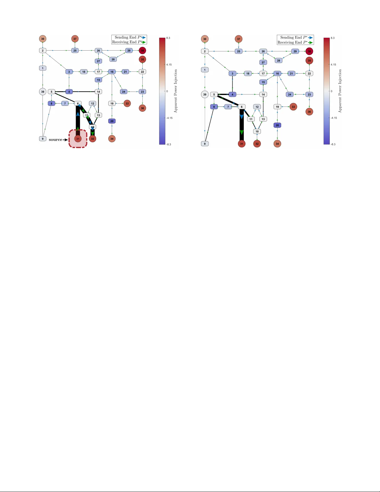
Authors: Samuel Chevalier, Petr Vorobev, Konstantin Turitsyn
1 A P assi vity Interpretation of Ener gy-Based F orced Oscillation Source Location Methods Samuel Che valier , Student Member , IEEE, Petr V orobe v , Member , IEEE, K onstantin T uritsyn, Member , IEEE Abstract —This paper dev elops a systematic framework f or analyzing how low fr equency for ced oscillations propagate in electric power systems. Using this framework, the paper shows how to mathematically justify the so-called Dissipating Energy Flow (DEF) for ced oscillation source location technique. The DEF’ s specific deficiencies are pinpointed, and its underlying energy function is analyzed via incremental passivity theory . This analysis is then used to pro ve that there exists no pas- sivity transf ormation (i.e. quadratic energy function) which can simultaneously r ender all components of a lossy classical power system passive. The paper goes on to develop a simulation-free algorithm f or predicting the perf ormance of the DEF method in a generalized power system, and it analyzes the passivity of three non-classical load and generation components. The proposed propagation framework and performance algorithm are both tested and illustrated on the IEEE 39-bus New England system and the WECC 179-b us system. Index T erms —F orced oscillations, inverse problems, passivity , phasor measurement unit (PMU), power system dynamics. I . I N T RO D U C T I O N F ORCED oscillations (FOs) are still a problematic reality in modern electric power systems. Caused by extraneous periodic perturbations, FOs can compromise system security , degrade system performance, and resonantly excite poorly damped interarea modes [1]–[3]. Despite widescale deploy- ment of Phasor Measurement Units (PMUs) across the US high voltage transmission network, locating the sources of these FOs remains a challenging task due to their sporadic nature, speed of propagation, and inability to be predicted by the system operators’ dynamical models. Since the most effecti ve w ay for dealing with a FO is to locate the source and disconnect it from service [4], an ef fectiv e source location technique is an indispensable smart grid application. Of the many source location techniques currently a vailable in the academic marketplace [5], the so-called Dissipating Energy Flo w (DEF) method has enjoyed some of the most successful testing results, both in simulation environments [4] and in real-time applications [6]. The method was originally dev eloped by Chen et al. [7], but its underlying mathematics lev erage the L yapunov functions from [8]. Despite its suc- cess, when its underlying modeling assumptions are violated, the method may perform poorly [9]–[11]. Additionally , the method has lacked a generalized framework which is capable of providing a system-wide justification for its usage. This work was supported in part by the Skoltech-MIT Next Generation grant and by the MIT Energy Initiativ e Seed Fund Program. S. Chev alier is with Department of Mechanical Engineering, Massachusetts Institute of T echnology . E-mail: schev@mit.edu P . V orobe v is with the Skolkov o Institute of Science and T echnology (Skoltech), Moscow , Russia. E-mail: p.vorobe v@skoltech.ru K. Turitsyn was with Department of Mechanical Engineering, Mas- sachusetts Institute of T echnology . E-mail: turitsyn@gmail.com The primary challenge to reliable DEF performance is the contribution of dissipating energy from non-FO sources, such as lossy transmission lines, lossy or negati vely damped loads, and generator dynamics dominated by non-passive controllers. An actual example of this contribution may be found in Fig. 1 of [11]. If these contributions are large enough, the FO source can appear to be a dissipating energy sink and the DEF method can fail. Despite its inadequacies, the DEF’ s excellent performance in real-time application at ISO New England strongly implies that further research should be performed in order to more systematically characterize the method. Shortcomings of the DEF method have been analyzed in [9], and [11] has recommended using passivity theory to interpret the method from a new mathematical perspectiv e, but no theoretical methods have been devised for testing how the DEF method will perform in an arbitrary network. Such testing is essential in order to ensure that the DEF can perform adequately in new en vironments, such as in microgrids where “R/X” line ratios are high and voltage control is fast, or in networks that have particularly resisti ve load pockets. T o make such predictions, a systematic framework is needed in order to thoroughly study the DEF . Accordingly , this paper develops a framework which is suit- able for analyzing the DEF method via passivity theory in the context of a full-scale system. Initially , this framew ork is used to analyze a lossy classical power system, but the methods are then generalized to include arbitrary system models; these generalized methods are thus capable of inv estigating all of the problematic effects presented by lines, loads and generator controllers. The primary contributions of this paper are as follows: 1) Using the Frequency Response Function (FRF) analysis proposed in [10], we lev erage a variety of tools from A C circuit theory in order to dev elop a linearized framework for analyzing oscillation propagation at the system lev el. 2) W e subsequently use the proposed framework, along with the passivity observations from [11], to theoretically justify the DEF method and show that there exists no other quadratic passi vity transformation which will render all components of the entire network passi ve in a classical power system. 3) A simulation-free algorithm is developed which predicts the performance of the DEF method in a generalized power system. 4) The proposed passivity transformation is used to analyti- cally in vestigate the dissipating energy flo w properties of three common, yet non-classical, grid components. The remainder of this paper is structured as follows. In Section II, we deri ve the linearized propagation framew ork 2 and show how quadratic energy is conserved in the system. In Section III, we extend the energy function analysis and prov e that there is no quadratic energy function which will render all components of a classical power system passiv e. W e then leverage the proposed framework in Section IV in order to dev elop an algorithm which analytically predicts the performance of the DEF method for a generalized power system. W e present illustrativ e and supportiv e test results in Section V and of fer concluding remarks in Section VI. I I . P E RT U R BAT I V E N E T W O R K M O D E L D E R I V A T I O N In this section, we introduce a linearized network model which is particularly useful for analyzing FO propagation in power systems. W e refer to it as a “perturbati ve” model since it captures the network’ s response to small 1 perturbations. A. Complex Admittance Matrices W e consider a power system component, sho wn in Fig. 1, whose dynamics are gov erned according to the D AE set ˙ x = f ( x , u , u v ) (1a) y = g ( x , u , u v ) , (1b) where inputs u v = [ V r , V i ] and outputs y = [ I r , I i ] are vec- tors of real and imaginary voltages and currents, respectiv ely . Fig. 1. DAE modeled component tied to a larger power system. W e linearize this model around a steady state operating point to linearly relate the voltage and current perturbations: ∆ ˙ x = A ∆ x + B ∆ u v (2a) ∆ y = C ∆ x + D ∆ u v . (2b) Assuming (2) is BIBO stable, its Fourier transform admits the Frequency Response Function (FRF) of the component [10]: ˜ y = C ( j Ω 1 − A ) − 1 B + D | {z } Y ( j Ω) ˜ u v , (3) where Ω is the angular frequency of the input and output signals, and Y ≡ Y ( j Ω) ∈ C 2 × 2 is referred to as the admittance matrix relating voltage ˜ u v ∈ C 2 × 1 and current ˜ y ∈ C 2 × 1 perturbations. These perturbations can be given in rectangular ( ˜ V r , ˜ V i ) or polar ( ˜ V , ˜ θ ) coordinates depending on con venience. In this paper , we will primarily consider the effects of the FRF matrix at the relev ant forcing frequency Ω d of the FO. When referring to Y , we will use the terms FRF and admittance interchangeably , depending on the context. 1 The framework presented in this paper is valid when FOs are sufficiently “small”, such that quadratic nonlinearities may be neglected. B. Network Modeling Consider a power system network whose graph G ( V , E ) has edge set E , |E | = m , verte x set V , |V | = n , and directed nodal incidence matrix E ∈ R m × n [12]. In power system modeling, it is standard practice to use the incidence matrix to build the nodal admittance matrix Y bus from the primitiv e admittance matrix Y p via Y bus = E † Y p E [13]. This procedure is possible because the admittances in Y p are complex values ∈ C 1 . In the following analysis, all admittances in the form of (3) must be expressed in 2 × 2 matrix form (i.e. Y ∈ C 2 × 2 ). Accordingly , we need an incidence matrix which can relate 2 × 2 , rather than 1 × 1 , admittance values. W e thus build a so-called “augmented” incidence matrix E a ∈ R 2 m × 2 n . This matrix is constructed by taking E and replacing all values of 1 with the 2 × 2 identity matrix 1 2 and all v alues of 0 with a 2 × 2 zero matrix 0 : E = 1 − 1 · · · 0 1 . . . . . . ⇔ E a = 1 2 − 1 2 · · · 0 1 2 . . . . . . . (4) Considering voltage and current perturbation phasors such as ˜ u v and ˜ y from (3), we define the vector V b ∈ C 2 n × 1 as the vector of rectangular bus voltage perturba- tion phasors, and we define the vector I l ∈ C 2 m × 1 as the vector of rectangular line current perturbation phasors, where the con vention of the positi ve line current flows agrees with the direction of the augmented incidence matrix: V b = ˜ V r, 1 ˜ V i, 1 . . . ˜ V r,n ˜ V i,n , (5) I l = ˜ I r, 1 ˜ I i, 1 . . . ˜ I r,m ˜ I i,m . (6) Admittance matrices Y l, 1 , ..., Y l,m , Y l,i ∈ R 2 × 2 , associated with the m transmission lines, are placed diagonally in the matrix Y L ∈ R 2 m × 2 m such that Y L = Y l, 1 0 . . . 0 Y l,m . (7) T ransformers with off-nominal tap ratios, such as tap changing transformers, are discussed in Appendix A. Line current and bus voltage perturbations obey Ohm’ s law: Y L E a V b = I l . (8) Admittance matrices Y s, 1 , ..., Y s,n , Y s,i ∈ C 2 × 2 , associated with shunt elements at each of the n buses, are placed diagonally in the matrix Y S ∈ C 2 n × 2 n , such that Y S = Y s, 1 0 . . . 0 Y s,n . (9) These shunt admittances are not simply capacitors or in- ductors; they can represent generators, loads, or any other terminal element in the system and can be constructed via (3). If multiple elements are connected in parallel, such as a generator and its station load, their admittances can be modeled independently and summed to compute the aggreg ate 3 shunt admittance. The shunt matrix Y S may be used to compute the shunt current injections 2 I s ∈ C 2 n × 1 via I s = Y S V b . (10) As outlined in [10], when analyzing a network with this representation, FOs show up like current sources at their respectiv e source buses. For a system experiencing a single FO, there will be a single current source I ∈ C 2 × 1 driving the entire network. W e define a sparse FO vector of current injections J ∈ C 2 n × 1 whose structure will take the form J = [ 0 , . . . 0 , I , 0 , . . . 0 ] > . (11) If bus k is the source of the FO, then I will be located in elements J 2 k − 1 and J 2 k . Source injections in J obey the same current con vention as I s . The network obeys KCL, i.e., all nodal currents sum to 0: J + I s + E † a I l = 0 . (12) W e define I I ≡ E † a I l to be the aggregate current injection at each node: it represents the sum of the source current injection at each bus plus the shunt current flowing to ground. V ia conservation of current at each bus, we have − J = I I + I s (13a) = E † a I l + Y S V b (13b) = E † a Y L E a + Y S V b . (13c) The block-Hermitian dynamic nodal admittance (or augmented dynamic Y -bus) matrix Y B ∈ C 2 n × 2 n is this defined to be Y B = E † a Y L E a + Y S . (14) Assuming there is a single FO in the system, it is instructiv e to rewrite (13c) with partitioned matrices and vectors, where the system has been renumbered such that the source bus is bus 1, and the current injection has a value of I ∈ C 2 × 1 : − J = Y B V b (15a) − I 0 = Y B 1 Y B 2 Y B 3 Y B 4 V s V ns , (15b) where V s ∈ C 2 × 1 represents v oltage perturbations at the source bus, V ns ∈ C (2 n − 2) × 1 represents voltage perturbations at all other buses, and V b = V _ s V ns . While I represents the true source current injection, we may also define I 0 as the sum of the source current at the source b us plus its shunt injection: I 0 = I + Y s, 1 V s . (16) Correspondingly , we say that Y 0 B 1 contains no shunt element, and I 0 is the current directly measur ed at the source bus flowing into the network ; we note that it is equal to the first two elements of I I . W e now restate (15a)-(15b) with this update: − J 0 = Y 0 B V b (17a) − I 0 0 = Y 0 B 1 Y B 2 Y B 3 Y B 4 V s V ns . (17b) 2 Shunt currents flowing out of the circuit to ground are defined as positi ve. A simple Kron reduction can be performed in order to deter - mine the ef fectiv e admittance “seen” by the current source: − I 0 = Y 0 B 1 − Y B 2 Y − 1 B 4 Y B 3 | {z } Y N V s , (18) where Y N ∈ C 2 × 2 is a 2 × 2 complex aggregate network admittance matrix and V s is the resulting voltage caused by the current injection I 0 interacting with the aggregate network dynamics codified in Y N . In this model, since voltage pertur- bations are considered a response to rouge current injections, it is helpful to re write (18) with voltage as a function of current: V s = −Z N I 0 , (19) where Z N = Y − 1 N is the aggregate network impedance. In other words, the current injection I 0 gives rise to the network voltages, and the vector V b in (17a) is not arbitrary: the Kron reduction of (18) is only meaningful when V b acts as a solu- tion to the linear system − J 0 = Y 0 B V b , i.e. V b = − ( Y 0 B ) − 1 J 0 . Definition 1. W e r efer to the admittance matrix Y N of (18) as the system’ s dynamic W ar d equivalent ( D WE ) admittance. C. Quadratic Ener gy Considerations As with any network which obeys Kirchhoff ’ s laws, T el- legen’ s theorem is also obeyed: the sum of the products of branch (including shunt branches) potential differences and branch flo ws is equal to 0. Accordingly , 0 = ( E a V b ) † I l + V † b ( I s + J ) (20a) = V † b E † a I l + I s + J (20b) = V † b ( Y B − Y B ) V b , (20c) where (20a) is the statement of T elle gen’ s theorem, (20b) is the conservation of current, and (20c) is the resulting proof. As a consequence of this theorem, there exist a family of quadratic functionals for which conservation laws can be formulated. An obvious one is the “real power”, Re { VI † } , that is consumed only on the elements with positiv e resistance. In the context of FOs, an alternativ e interpretation of the conserv ation of power can be acquired by manipulating (17b) in order to define another (arbitrary) type of quadratic power 3 . The key observation is that this new quadratic power will be conserved throughout the network. T o show why , we consider matrix Q ∈ C 2 n × 2 n with block diagonal sub-matrices Q b ∈ C 2 × 2 : Q = Q b 0 . . . 0 Q b . (21) W e no w left multiply (17a) by V † b Q , which represents the application of a quadratic energy function: − V † b Q J 0 = V † b QY 0 B V b (22a) − V † s Q b I 0 = V † b Q E † a Y L E a V b + V † b ( QY 0 S ) V b . (22b) 3 The term “quadratic power” is used since we are multiplying voltages and currents, but the quadratic quantity doesn’t necessarily hav e the interpretation of physical po wer . It can also be interpreted as an “energy function”. Quadratic energy and quadratic power are therefore used interchangeably . 4 Different choices for matrix Q b correspond to different energy function applications, but in each case, the quadratic quantity is conserved. For example, if Q b is chosen such that Q b = 0 − 1 j Ω 1 j Ω 0 , (23) then the associated energy function corresponds to the DEF method [11]. Under DEF assumptions, lines and loads are rendered lossless, i.e ( Q b Y ) + ( Q b Y ) † = 0 . Thus, in taking the real part, (22b) simplifies to Re { V † s Q b I 0 } | {z } Source Energy + n X i =2 Re { V † ns,i ( Q b Y s,i ) V ns,i } | {z } Generator Damping Contributions = 0 , (24) where V s and V ns,i are the source and i th non-source bus voltage perturbation vectors, respectiv ely . The formulation of (24) further clarifies the DEF’ s functionality: since all the damping energy consumed by generators is positiv e [11], the source energy is necessarily neg ativ e and can be traced back to the single, negati ve source. The DEF technique, therefore, is based on tracking a particular type of quadratic power in the network. When constructing the system’ s quadratic energy function, we are not restricted to choosing just a Q matrix. W e may also introduce matrix P whose structure matches Q . For example, we may set U b = P − 1 V b , left multiply (17a) by U † b Q , and insert a P P − 1 term. Updating (24) yields: Re { U † s Q b I 0 } | {z } Source Energy + n X i =2 Re { U † ns,i ( Q b Y s,i P b ) U ns,i } | {z } Generator Damping Contributions = 0 . (25) I I I . E N E R G Y F U N C T I O N A N A L Y S I S The DEF method can be interpreted as the application of a specific quadratic energy function to all elements of a network. Reference [11], which revie ws relev ant passivity concepts, explains how this quadratic energy function can be interpreted as a matrix transformation (called a “passi vity transformation”) which attempts to render system elements incrementally pas- siv e. Generally , a passiv e component is one which can only dissipate and store, but not produce, physical power . T o av oid confusion, we point out that this paper discusses the so-called incr emental passivity , which refers to the passi ve nature of a system’ s incremental change from its equilibrium, as defined by [14, eq. (4.159)]. This is also known as “shifted passivity”. W e stress that physical passivity of an element does not imply incremental passivity when some transformation, such as (21), has been applied. In the remainder of the paper , the term passivity always refers to incremental passivity . Reference [11] further shows that the DEF energy function is inadequate for lossy network elements. While it may be tempting to dev elop a new passi vity transformation which is suitable for lossy networks, in this section, we use passivity theory to prov e that no constant quadratic energy function exists for the classical model of a multimachine power system. For coherency , we first offer the following clarification of how we use the terms “lossy” and “lossless” in this paper . Definition 2. In keeping with the con ventional nomenclature for both power systems and passivity literatur e, we offer the following definitions for lossy and lossless: • Lossy : A lossy element is an element which contains r esistance; a lossy system is a system which contains r esistive transmission lines. • Lossless 4 : The term lossless describes a FRF whose Hermitian part is 0 . If Y + Y † = 0 , Y is said to be lossless; if M Y + ( M Y ) † = 0 , M Y is said to be lossless. A. Basis Matrices T o aide in the energy function analysis and inference techniques, we define a useful set of basis matrices. Definition 3. W e define orthogonal ( A − 1 = A † ) basis matrices T 1 = 1 0 0 1 , T 2 = 1 0 0 − 1 , T 3 = 0 1 1 0 , T 4 = 0 − 1 1 0 , and the set T = { T 1 , T 2 , T 3 , T 4 } . Set T spans r e gion R 2 × 2 : span ( T ) = ( 4 X i =1 λ i T i T i ∈ T , λ i ∈ R 1 ) = R 2 × 2 . (26) Lemma 1. Ther e exists no non-singular matrix Γ ∈ C 2 × 2 for which, simultaneously , Re v † T i Γ v ≥ 0 , ∀ v ∈ C 2 × 1 , ∀ i ∈ { 1 } (27) Re v † T i Γ v = 0 , ∀ v ∈ C 2 × 1 , ∀ i ∈ { 2 , 3 , 4 } . (28) Pr oof. W e write Γ as the sum of its diagonal ( Γ d ) and off- diagonal ( Γ o ) component matrices: Γ = Γ d + Γ o . Since Re { v † ( T i Γ) v } = 0 , ∀ v ∈ C 2 × 2 is equiv alent to stating that T i Γ + ( T i Γ) † = 0 , the constraints on Γ caused by T 2 , T 3 , and T 4 from (28) may be stated as T 2 → Γ d = − Γ † d , Γ o = Γ † o , (29) T 3 → K Γ d = − Γ † d K, K Γ o = − Γ † o K, (30) T 4 → K Γ d = Γ † d K, K Γ o = − Γ † o K, (31) where K ≡ T 3 is defined to be the reversal matrix in [15]. Ac- cordingly , Γ d must be simultaneously skew-Hermitian, skew- perhermitian and perhermitian, respectively [15]. Necessarily , Γ d = 0 . The matrix Γ o must be simultaneously Hermitian and skew-perhermitian. Necessarily , j β T 4 , β ∈ R 1 , is the only matrix which fits this description. W e define Γ ? = j β T 4 (32) as the only matrix which uniformly satisfies (28). W e apply Γ = Γ ? to (27) and consider the eigen values of the matrix T 1 Γ ? + T 1 Γ ? † = 2 β j T 4 : det 2 β j T 4 − diag { λ } = λ 2 − 4 β 2 , (33) λ = ± 2 β (34) which violates (27). Since T 1 Γ ? + ( T 1 Γ ? ) † is an indefinite matrix but Γ ? is the only matrix which satisfies (28), the theorem has been prov ed. 4 While “lossless” certainly can also refer to a transmission network with purely reactive lines, we do not in voke that definition anywhere in this paper . 5 Corollary 1. Γ ? is a solution to P Γ ? + ( P Γ ? ) † = 0 for any matrix P which may be written as P = P 4 i =2 α i T i , α i ∈ R 1 . Corollary 2. The results of Lemma 1 stand if T i is right multi- plied by transformation matrix M instead of left multiplied by transformation matrix Γ . There exists no non-singular matrix M ∈ C 2 × 2 for which the following simultaneously hold: Re v † M T i v ≥ 0 , ∀ v ∈ C 2 × 2 , ∀ i ∈ { 1 } (35) Re v † M T i v = 0 , ∀ v ∈ C 2 × 2 , ∀ i ∈ { 2 , 3 , 4 } (36) Corollary 3. By employing both non-singular matrices Γ ∈ C 2 × 2 and M ∈ C 2 × 2 , the solution to Re v † M T i Γ v = 0 , ∀ v ∈ C 2 × 1 , ∀ i ∈ { 2 , 3 , 4 } (37) must take the form Γ = ( j β T 4 ) M † for any M ∈ C 2 × 2 . This may be seen via the following manipulation: 0 = M T i Γ + ( M T i Γ) † , ∀ i ∈ { 2 , 3 , 4 } (38a) = T i (Γ M † − 1 ) + ( M − 1 Γ † ) T † i , ∀ i ∈ { 2 , 3 , 4 } . (38b) Since (38b) may only be solved by Γ M † − 1 = j β T 4 , per Lemma 1, we have that Γ = ( j β T 4 ) M † must be satisfied. B. Quadratic Ener gy Functions in a Classical P ower System W e no w assume the classical model of a lossy multimachine power system model [16] and allow for constant power loads to be present. The forms of the FRFs associated with constant power loads ( Y p ), constant impedance lines/shunts ( Y z ), and classical generators ( Y g ) are given in [11]. The set of plausible FRFs associated with these three elements may be constructed according to the follo wing basis matrix combinations: Y p = X i =2 , 3 a i T i , a i ∈ R 1 (39a) Y z = X i =1 , 4 a i T i , a i ∈ R 1 (39b) Y g = X i =2 , 3 , 4 ( a i + j b i ) T i , a i , b i ∈ R 1 . (39c) The FRF of a classical generator is derived and fully explained in [10], and, for con venience, is explicitly re-stated here: Y g = γ (Ω) sin( δ ) cos( δ ) − cos 2 ( δ ) sin 2 ( δ ) − sin( δ ) cos( δ ) | {z } T δ + " 0 1 X 0 d − 1 X 0 d 0 # | {z } T X (40) γ (Ω) = E 0 2 X 0 2 d M ( j Ω) 2 + V t E 0 X 0 d cos( ϕ ) − j (Ω D ) V t E 0 X 0 d cos( ϕ ) − M Ω 2 2 + (Ω D ) 2 . (41) where δ is the generator’ s absolute rotor angle and γ ≡ γ (Ω) ∈ C 1 is a complex frequency dependent parameter . Matrix ( 40 ) has many useful properties, one of which will be addressed in subsection III-C. Giv en that any admittance matrix Y may be written as the complex sum of the four weighted basis matrices, we introduce the follo wing useful definition: Definition 4. W e assume some admittance Y may be writ- ten as Y = P 4 i =1 ( a i + j b i ) T i . Using matrices M and Γ fr om Cor ollary 3, where Γ = ( j β T 4 ) M † , we define P ? = Re { u † ( M Y Γ) u } as the dissipating po wer for input vector u . W e further define two other types of quadratic power: resistive pow er P ? r and damping power P ? d , where P ? = P ? r + P ? d , and • P ? r = Re u † M a 1 T 1 Γ u • P ? d = Re u † M j b 2 T 2 + j b 3 T 3 + j b 4 T 4 Γ u . W e now prov e that a perturbativ e system model containing elements (39a)-(39c) cannot be rendered passiv e under any quadratic passivity transformation. In other words, there is no quadratic quantity that is dissipated by all elements present in common networks. Theorem 1. There exist no non-singular matrices M ∈ C 2 × 2 and Γ ∈ C 2 × 2 for which M Y Γ + ( M Y Γ) † 0 , ∀Y ∈ {Y p , Y z , Y g } . (42) Pr oof. The FRF of a strictly reactiv e element, such as matrix T X in (40), is ∝ T 4 while the FRF of a strictly capacitiv e element is ∝ − T 4 . The only way for M T 4 Γ + M T 4 Γ † 0 and − M T 4 Γ − M T 4 Γ † 0 to be simultaneously true is for M T 4 Γ + M T 4 Γ † ≡ 0 . Since both reacti ve and capacitiv e elements appear in classical power systems, T 4 must be lossless under the desired passi vity transformation. W e now consider some classical generator whose damping characteristics are sufficiently small ( D ≈ 0 ), such that γ is a real parameter . In this case, the matrix M Y g Γ + ( M Y g Γ) † reduces to M γ T δ Γ + ( M γ T δ Γ) † since T X must be a lossless element according to the pre vious conclusion about T 4 . W e define the squared electromechanical resonant frequenc y associated with the classical generator as Ω 2 r = VE 0 M X 0 d cos( ϕ ) . For some , γ (Ω r − ) = − γ (Ω r + ) . W e must therefore ensure that M γ T δ Γ + ( M γ T δ Γ) † 0 and − M γ T δ Γ − ( M γ T δ Γ) † 0 , respectiv ely , when ensuring the generator’ s passivity on either side of the resonant peak. The only way for these state- ments to be simultaneously true is for M T δ Γ + ( M T δ Γ) † ≡ 0 . T o accomplish this, we consider the numerical structure of T δ for two plausible rotor angle values: δ 1 = 0 and δ 2 = π 4 : T δ ( δ 1 ) = 0 − 1 0 0 = 1 2 T 4 − T 3 , (43) T δ ( δ 2 ) = 1 2 − 1 2 1 2 − 1 2 = 1 4 T 2 + T 4 . (44) Since M T 4 Γ + M T 4 Γ † ≡ 0 , then we must also require M T 3 Γ + M T 3 Γ † ≡ 0 from (43) and M T 2 Γ + M T 2 Γ † ≡ 0 from (44) in order to ensure that M T δ Γ + ( M T δ Γ) † ≡ 0 . W e are thus requiring that Re ˜ v † M T i Γ ˜ v = 0 , ∀ ˜ v ∈ C 2 × 1 , ∀ i ∈ { 2 , 3 , 4 } . As stated in Corollary 3, the only way to achieve losslessness for basis matrices 2, 3 and 4 is for Γ = ( j β T 4 ) M † . By employing this transformation, Lemma 1 prov es that the quadratic energy associated with any element containing T 1 will be rendered indefinite in sign. Since (39b) contains T 1 when resistance is present in the network, then there exists no nonsingular matrices M and Γ for which M Y Γ + ( M Y Γ) † 0 , ∀Y ∈ {Y p , Y z , Y g } . Corollary 4. By choosing M = T 1 , β = − 1 Ω , and Γ = ( j β T 4 ) M † , we arrive at the passivity transformation implic- itly employed by the DEF , as given by [11, eq. (38a,b)]. 6 Corollary 5. The passivity transformation Γ = ( j β T 4 ) M † r enders constant power and reactive (capacitive or inductive) elements of the system lossless, classical generators passive (see [11, eq. (49)]), and r esistive elements non-passive. W ith- out r esistive elements, the DEF method is a fully r eliable sour ce location technique in classical power systems. Corollary 6. Since the linearized admittance matrix Y asso- ciated with any ZIP load is pur ely r eal, i.e. Y = Re {Y } , the eigen values of its transformed Hermitian part will be equal and opposite in value: λ ( M Y Γ + ( M Y Γ) † ) = ± α , wher e α = 0 for constant power or purely r eactive loads. If a network has no resistiv e elements and is truly passi ve, no quadratic energy production can occur on regular network elements, so injections of energy hav e to be related to external sources, like FOs. This is why finding a passiv e energy- like form is important, and why the almost-passive form used by DEF has had so much success. T o further show why the results of Theorem 1 are problematic for the DEF method, we consider the structure of (24): since the generator damping contributions are positive definite, the source energy is necessarily negati ve in a po wer system with no resistance. This is not true in a lossy po wer system. T o show why not, we define block matrices M ∈ C 2 n × 2 n and Γ ∈ C 2 n × 2 n , where M = M 0 . . . 0 M , Γ = Γ 0 . . . 0 Γ , and whose block diagonal matrices are giv en by M and Γ = ( j β T 4 ) M † , respectiv ely . W e left multiply (17a) by M and insert ΓΓ − 1 on the RHS: − MJ 0 = M E † a Y L E a + Y 0 S ΓΓ − 1 V b . (45) Defining the transformed voltage vectors U b = Γ − 1 V b and U s = Γ − 1 V s , we left multiply (45) by U † b and simplify . W e may group the dissipating power injections into their respectiv e contrib uting groups (assuming lossless loads): 0 = U † s M I 0 | {z } Source + U † b ( M Y 0 S Γ) U b | {z } Generator + U † b ( M E † a Y L E a Γ) U b | {z } Network . (46) The FO source term can produce only negati ve damping energy , i.e. Re { U † s M I 0 } < 0 , if the condition M Y 0 S + E † a Y L E a Γ + M Y 0 S + E † a Y L E a Γ † 0 (47) is met. If it is not met, indefinitely signed resistiv e energy can dominate damper winding energy absorption and the source term can, in fact, appear as a positiv ely damped element. In this plausible situation, the DEF method will fail. W e note that violation of (47) is a necessary but not sufficient condition for DEF failure. Next, we show that the sign of the injected resistiv e energy associated with a transmission network can be negated if all system voltages are complex conjugated. Theorem 2. Consider a lossy transmission network (just the network). F or any transformed voltage vector U b which yields quadratic energy Re { U † b ( M ( E † a Y L E a )Γ) U b } = P ? r , ther e exists conjugated vector U ∗ b which yields an equal and oppo- site quadratic ener gy Re { U ∗† b ( M ( E † a Y L E a )Γ) U ∗ b } = − P ? r , wher e M and Γ , with submatrices M and Γ , yield from Cor ollary 3. Pr oof. W e split the transmission line matrix into its conducti ve and susceptiv e parts: Y L = Y ¯ G + Y ¯ B , where Y ¯ G,i = G i T 1 and Y ¯ B ,i = B i T 4 . W e also define block matrices M = j T 4 Γ and Γ = T 1 from M and Γ . Therefore, M E † a Y L E a Γ = M E † a ( Y ¯ G + Y ¯ B ) E a . The Hermitian part (termed H ) is H = M E † a ( Y G + Y Bx 2 ) E a + E † a ( Y G −Y Bx 2 ) E a M † (48a) = M E † a Y G 2 E a + E † a Y G 2 E a M (48b) = M E † a Y G E a (48c) where the matrices of (48b) commut e since the product of Her - mitian matrices is also Hermitian. W e define G ij ≡ j G ij T 4 , where G ij is the scalar line conductance connecting buses i and j , and u i ⊂ U b is the voltage element of U b associated with bus i . From (48c), the quadratic power is P ? r = n X i =1 u † i ( X j 6 = i G ij ) u i − n X j 6 = i n X i 6 = j u † i T 4 G ij u j (49a) = X i,j ∈E ( u † i G ij u i + u † j G ij u j − u † i G ij u j − u † j G ij u i ) (49b) = X i,j ∈E ( u i − u j ) † G ij ( u i − u j ) | {z } u ij . (49c) The quadratic quantity x † G ij x = may be negated by conjugating the input (proof tri vial): x ∗† G ij x ∗ = − . By taking U ∗ b as an input to Re { MU ∗† b ( E † a Y G E a ) U ∗ b } , by (49c) we thus hav e P i,j ∈E u ∗† ij G ij u ∗ ij = − P ? r . W e note that U b cannot be chosen arbitrarily; it must represent a valid solution to the linear system of (17a). Since U b is not itself a degree of freedom but rather a response to some current injection, statements about the mathematical characteristics of M Y N Γ + ( M Y N Γ) † are dif ficult to prove using energy-based arguments. Despite this fact, the following two theorems offer useful insights into these characteristics. First, we of fer a definition of an associated system. Definition 5. Consider classical power system Σ c with ZIP loads, passive generator s, and a lossy transmission network. This system’ s voltage vector V b is V b = V _ s V ns , wher e V ns = −Y − 1 4 Y 3 V s fr om (17b). All voltage vectors are trans- formed such that U = Γ − 1 V . The Kr on r educed admittance (D WE) seen by a FO sour ce is Y N as in (18). The matrix N c = 1 2 ( M Y N Γ) + 1 2 ( M Y N Γ) † , with matrices M and Γ fr om Corollary 3, will have two eigen values: λ 1 and λ 2 . Theorem 3. Consider N c fr om Σ c : ( a ) If condition (47) is met, λ 1 , λ 2 > 0 . ( b ) If Re { U † s M I 0 } > 0 is measur ed, i.e. the DEF method has failed, condition (47) is violated and λ 1 ∨ λ 2 < 0 . Pr oof. By modifying (46), we have − U † s M I 0 = U † b M ( Y 0 S + E † a Y L E a )Γ U b , and with condition (47) met, − U † s M I 0 > 0 . Since − I 0 = Y N V s , we hav e that U † s M Y N Γ U s > 0 by substitution, implying that λ { ( M Y N Γ) + ( M Y N Γ) † } > 0 , ∀ λ ∈ { λ 1 , λ 2 } , proving proposition ( a ) . If Re { U † s M I 0 } > 0 , then U † s N c U s < 0 is directly implied. Accordingly , λ 1 ∨ λ 2 < 0 . By the conservation argument 7 presented in the proof of proposition ( a ) , if U † s N c U s < 0 , then Re { U † b M ( Y 0 S + E † a Y L E a )Γ U b } < 0 implying the violation of condition (47), proving proposition ( b ) . Our final theorem characterizes how the eigen values change as resistance is added to Σ c . Theorem 4. Consider N c fr om Σ c . No amount of additional r esistance to lines or loads can cause the eigen values of N c to both become ne gative: if det( N c ) ≥ 0 then trace( N c ) ≥ 0 . Pr oof. Consider some altered version of Σ c where all resis- tance has been removed from the system. In this situation, λ 1 , λ 2 ≥ 0 according to Theorem 3. Consider some secondary altered version of Σ c where generators hav e no damping (making them “lossless”). In this situation, matrix Y N will be purely real ( Y N ∈ R 2 × 2 ) via (18). Therefore, assuming lossy lines, λ 1 = − λ 2 6 = 0 . All real systems exist between these two alternatives. W e now consider a system with nominal resistance and some value α which parameterizes the amount of damping in the system generators ( α = 0 corresponds to no damping). When α = 0 , λ 1 = − λ 2 6 = 0 . As α → ∞ , then λ 1 , λ 2 → R + . In between these extremes, if for some value of α > 0 , there is λ 1 , λ 2 ∈ R − , then it would imply that the addition of positiv e damping causes the system to lose the ability to dissipate the quadratic energy which the generator damping consumes. This is a contradiction, so at least one eigen value must always remain positi ve for all levels of damping and resistance. Remark 1. Since the D WE Y N is the admittance of the network “seen” by the sour ce, the ne gative D WE −Y N is the admittance “seen” by the network behind the source b us. By Theor em 4, the eigen values of N c = 1 2 ( M Y N Γ) + 1 2 ( M Y N Γ) † can never be simultaneously ne gative. Stated differ ently , the eigen values of − N c can never be simultaneously positive. F or this reason, the admittance seen by the network behind the FO source can never be truly passive. C. Infer ence Analysis Observations If a system-wide admittance matrix model, i.e. (14), is fully known at the time of a FO ev ent, locating the source of the FO is trivial once PMU measurements are obtained. Such a model is often unknown or poorly known in real time, so model based approaches aren’t typically applicable. Using PMU inference methods to build the admittance model (in real time) are thus a tempting solution. Unfortunately , the system is inherently underdetermined. In a standard linear circuit, admittance may be computed as the simple ratio of complex inputs and complex outputs. This cannot be done in a MIMO system. Assuming complex input ( ˜ u v ) and output ( ˜ y ) vectors for the system in (3) are given, a generalized admittance Y ∈ C 2 × 2 cannot be directly inferred since (3) represents four real linear equations while Y is specified with 8 coef ficients ( a i , b i , i ∈ { 1 , 2 , 3 , 4 } ): Y 1 Y 2 Y 3 Y 4 = 4 X i =1 ( a i + j b i ) T i . (50) The system is thus se verely underdetermined. For a classical generator , though, this is not the case. This is an important observation, because the dynamics of a system experiencing a FO are dominated by the electromechanical response of synchronous generators. Proposition 1. The admittance Y g of a classical generator can be uniquely specified as the weighted sum of six basis matrices with only four real coefficients. Pr oof. It may be observed that Y g in ( 40 ) contains no complex combination of basis matrix T 1 . Therefore, Y g may be written using six basis matrix coef ficients a i , b i , i ∈ { 2 , 3 , 4 } via Y g = P i =2 ... 4 ( a i + j b i ) T i . W e further observe that for ( a 2 + j b 2 ) T 2 and ( a 3 + j b 3 ) T 3 , the ratios of a 2 /b 2 and a 3 /b 3 must be equal, so a 2 = b 2 a 3 /b 3 . This eliminates one coefficient. Finally , we write γ = γ r + j γ i and observe that b 2 = γ i sin( δ ) cos( δ ) while b 3 + b 4 = γ i sin 2 ( δ ) and b 3 − b 4 = − γ i cos 2 ( δ ) . Solving this system yields b 4 = + p b 2 2 + b 2 3 (assuming damping D is positive). Therefore, Y g may be specified with just four coef ficients: a 3 , a 4 , b 2 , and b 3 . Corollary 7. F rom Pr oposition 1, classical generator admit- tance Y g can be specified with only four parameter s. Thus, the infer ence pr oblem min Y g { ˜ y − Y g ˜ u v } r epr esents 4 equations and 4 unknowns and is thus a “determined” problem. In other words, the admittance of a classical generator can be fully inferred from PMU data. I V . P R A C T I C A L A P P L I C AT I O NS O F P A S S I V I T Y A N A L Y S I S In this section, we expound three practical applications of the analysis presented in this paper . First, we explicitly state how to implement the DEF source location method via the proposed frequency domain methods. Second, we show how system operators can use the proposed frame work to predict how the DEF method will perform in their respective networks without performing simulations. And third, we e xplain ho w the tools in this paper can be used to understand how the addition of new grid components will affect performance of the DEF method. In all further analysis, we assume M = 0 j − j 0 . (51) A. Ener gy Flow Calculations in the F requency Domain In order to compute the dissipating power signal P ? in a system which is experiencing a FO event, we con vert voltage and current PMU data into rectangular coordinates. Next, we take the Fast Fourier T ransform (FFT) of these signals, thus constructing ˜ V (Ω) = [ ˜ V r (Ω) , ˜ V i (Ω)] > and ˜ I (Ω) = [ ˜ I r (Ω) , ˜ I i (Ω)] > at all rele vant b uses and lines. Finally , we ev aluate these signals at the forcing frequency Ω d in order to compute the dissipating power injection at each bus or flow along each line: P ? = Re { ˜ V (Ω d ) † M ˜ I (Ω d ) } . (52) Positiv e P ? flowing out of an element indicates the presence of a non-passiv e component (typically a FO source). W e refer readers to Appendix B for a discussion on the difficulties of dealing with rectangular coordinates in a realistic power system. Using this procedure, a map, such as the one presented in Fig. 3, can be constructed. 8 B. Pr edicting P erformance of DEF Source Location The implicit goal of the DEF method is to locate the source of negativ e damping in the system. When resistiv e elements are introduced to the network, the goal becomes obfuscated because the source may appear passive, and thus, positiv ely damped. By Remark 1 though, the negati ve D WE of the source cannot be physically passi ve. A key contribution of this paper recognizes that while generators continue to be physically passiv e, the source only appears 5 passiv e when the DEF method fails in a classical power system. Before system operators can consistently rely on using the DEF method for FO source location, it is important that they first test if the method will perform adequately in their respectiv e networks. Algorithm 1 clarifies the exact analytical procedure which can be used to test if the DEF method will perform successfully for any given bus in the network at any given FO frequency . W e note that this off- line analysis in not restricted to classical power systems: any system component can be incorporated so long as its dynamics can be analytically approximated and linearized. Additionally , the type of oscillation source is entirely arbitrary: the methods in Algorithm 1 predict the sign of the energy flowing from the source bus terminal as a function of how the system dynamically responds to the abstracted oscillation signal. It is thus similar to testing if condition (47) is violated. ST AR T 1 construct nonlinear model (1) for all shunt components and linearize to build admittance (3) 2 construct shunt admittance matrix (9), augmented incidence matrix (4) and line admittance matrix (7) 3 construct dynamic nodal admittance (14) for each plausible FO frequency Ω d do for each plausible source bus i do 1) remove shunt admittance Y s,i from Y S 2) partition network via (17) and perform Kron reduction via (18) to construct Y N 3) compute λ 1 , 2 = λ { M Y N + ( M Y N ) † } Assume bus i generates FO of frequency Ω d : if λ 1 , λ 2 ≥ 0 then DEF will succeed else if λ 1 , λ 2 ≤ 0 then DEF will be fail else DEF will perform unreliably end end end Algorithm 1: Reliability T est for Energy Flo w Methods C. Analysis of Additional Grid Components Until this point in the paper , only the elements of a lossy classical power system hav e been considered, but it is impor- tant for system operators to consider how the addition of new elements will effect energy-based source location methods. If newly added elements are non-passiv e, it is also important for 5 The transformed FRF will have one positiv e and one negativ e eigen value. system operators to test the degree of allo wed penetration from these elements before energy-based source location methods will fail. In this subsection, we present examples of passivity analysis applied to three non-classical elements: frequency dependent loads, droop-controlled in verter systems, and third order synchronous generators with first order Automatic V olt- age Regulators (A VRs). 1) F requency Dependent Load: Assuming power is an instantaneous function of voltage magnitude and frequency [17], we may write P ( t ) and Q ( t ) via P ( t ) = P 0 (V / V 0 ) α p ( ω /ω 0 ) β p (53a) Q ( t ) = Q 0 (V / V 0 ) α q ( ω /ω 0 ) β q , (53b) where ω = ω 0 + ˙ θ . Since we are interested in the lin- earized responses of (53a) and (53b), we ev aluate their partial deriv atives at equilibrium ( V 0 , ω 0 = 1 ). Assuming sinusoidal perturbations, phasor notation yields ˜ P ˜ Q | {z } ˜ S = α p V 0 P 0 β p P 0 α q V 0 Q 0 β q Q 0 | {z } Y a 1 0 0 j | {z } I j ˜ V ˜ θ | {z } ˜ V p (54) where ˜ ω = j ˜ θ . Employing matrix T 1 from Appendix B, we transform from polar to rectangular via ˜ V = T 1 ˜ V p in (54): ˜ S = Y a I j T − 1 1 ˜ V . (55) W e next consider perturbations of P = V r I r + I i V i and Q = V i I r − V r I i . Treating ¯ V i/r and ¯ I i/r as steady state v alues, we linearize and con vert to phasor notation: ˜ P ˜ Q = ¯ I r ¯ I i − ¯ I i ¯ I r | {z } A I ˜ V r ˜ V i | {z } ˜ V + ¯ V r ¯ V i ¯ V i − ¯ V r | {z } A V ˜ I r ˜ I i | {z } ˜ I . (56) By equating (55) and (56), ˜ I and ˜ V are directly related by ˜ I = A − 1 V Y a I j T − 1 1 − A I | {z } Y b ˜ V . (57) Finally , we set α p = α q = 0 to isolate the ef fects of frequency , and we compute eigen values λ 1 , 2 = λ { M Y b + ( M Y b ) † } : λ 1 , 2 = β p cos( ϕ ) ± q β 2 p 2 (1 + cos(2 ϕ ) ) + β 2 q 2 (1 − cos(2 ϕ ) ) I / V . (58) where ϕ = θ − φ . In setting β ≡ β p ≈ β q , (58) simplifies to λ 1 , 2 = β (cos( ϕ ) ± 1)V / I . (59) Since power factor is usually close to unity , this case of frequency dependent load is primarily passive for β > 0 because the positiv e eigen value will be far larger than the negati ve eigen value. Otherwise, if β p = 0 , then the load behav es like a resistor (equal and opposite eigenv alues), but if instead β q = 0 , then the load is truly passiv e for reasonable values of power factor . 9 10 -2 10 -1 10 0 10 1 F requency (hertz) -20 0 20 40 60 6 6 1 ; , = 0 6 1 ; , = 0 : 05 6 1 ; , = 0 : 1 6 1 ; , = 0 : 15 6 1 ; , = 0 : 2 6 2 ; , = 0 6 2 ; , = 0 : 05 6 2 ; , = 0 : 1 6 2 ; , = 0 : 15 6 2 ; , = 0 : 2 Fig. 2. Plot of the eigenv alues of M Y + ( M Y ) † , where Y is associated with the dynamics of a droop-controlled in verter . For α = 0 , the system is fully passive since both eigenv alues are positiv e. 2) Dr oop-contr olled In verter: W e consider the dynamics of a droop-controlled inv eter circuit; such circuits have the poten- tial to dominate distributed energy resource interconnections. As gi ven in [18], the circuit’ s impedance may be stated as Z = " R c + j Ω L c − X c − k q 1+ j τ Ω X c − k p τ Ω 2 − j Ω R c + j Ω L c # . (60) Associated parameters are explained in [18], but k p and k q are the acti ve and reacti ve power droop coef ficients, and R c is the virtual + coupling resistance. W e seek to analyze the passivity of this system. Rather then inv ert (60), we consider the passiv- ity of the impedance Z directly . Appendix C establishes the equiv alence of passivity classifications between an admittance Y and its associated impedance Z = Y − 1 for transformation matrix M . W e thus compute the Hermitian part of M Z : M Z + ( M Z ) † = 2 " k p Ω(( τ Ω) 2 +1) j R c − j R c k q τ Ω ( τ Ω) 2 +1 # . (61) Since τ , Ω , and the droop coefficients are all positiv e, if R c is small, then the eigen values of (61) are simply λ 1 , 2 ≈ k p 2 Ω(( τ Ω) 2 + 1) , k q 2 τ Ω ( τ Ω) 2 + 1 (62) and the system is effecti vely passive. If R c is not neglected, though, the eigen v alue expressions become more cumbersome. Using the parameter values suggested in [18], we plot λ 1 and λ 2 as R c is scaled via R c = αX c , α ∈ { 0 , 0 . 05 , 0 . 1 , 0 . 15 , 0 . 2 } , for the matrix M Y + ( M Y ) † (we plot admittance eigenv alues rather than impedance eigen values solely for graphical clarify). Fig. 2 shows the eigenv alues. Clearly , as coupling resistance decreases in value, the in verter behaves more passi vely . The DEF method will thus perform more successfully when virtual + coupling resistance is minimized. 3) Thir d Or der Generator with F irst Or der A VR: W e con- sider the dynamics of a third order synchronous machine with a first order AR V . The associated model [17] is stated by ˙ δ = ∆ ω (63a) M ∆ ˙ ω = P m − P e − D ∆ ω (63b) T 0 d 0 ˙ e 0 q = E f − ( X d − X 0 d ) i d − e 0 q (63c) T a ˙ E f = K a (V r − V) − E f , (63d) where V r is the voltage reference set point, V e j θ is the terminal voltage phasor , i d = ( e 0 q − e q ) /X 0 d , i q = e d /X q , e d = V sin( δ − θ ) and e q = V cos( δ − θ ) . Finally , P e = e d i d + i q e q . W e define output power variables P and Q as P = − P e and Q = − ( i d e q − i q e d ) 6 . In order to make analytical claims about the passivity of (63), we leverage the alternativ e DEF interpretation proposed in Appendix D. T o make the analysis tractable, we choose to linearize the model about the generator’ s unloaded equilibrium point (i.e. θ = δ , V = e q , e d = 0 , etc.). Although this configura- tion may be uncommon, the resulting linearized dynamics are sufficiently simplified for approximating generator passivity . Additionally , the resulting admittance matrix H is diagonal, so the eigenv alues of K † H + ( K † H ) † are trivial. W e compute H from Appendix D: H = Ω( j M Ω+ D ) DX q Ω+ j ( M X q Ω 2 − 1) 0 0 K a +1 − Ω 2 T a T 0 d 0 + j Ω ( T a + T 0 d 0 ) (Ω T a − j )( X d j − Ω T 0 d 0 X 0 d ) . (64) T aking the eigen values of K † H + ( K † H ) † is equiv alent to taking the imaginary parts of the diagonals of matrix H . The relationship between ˜ P and ˜ θ (i.e. λ 1 ) is thus passi ve if Ω D ≥ 0 . (65) This will be true if damping D is positive. Interestingly , when the generator is unloaded , the damping provided by the field winding is of second order and thus has no mathematical impact on passi vity between ˜ P and ˜ θ . V ia (64), the relationship between ˜ Q and ˜ V (i.e. λ 2 ) is thus passi ve if T 0 d 0 Ω 2 T 2 a + T 0 d 0 ( X d − X 0 d ) − K a ( T 0 d 0 X 0 d + X d T a ) ≥ 0 . (66) This result has many interesting interpretations. For K a small or T a sufficiently large, the expression will always be passive. Strong and fast A VR response thus causes the relationship between ˜ Q and ˜ V to lose passivity . For passivity to be guaranteed ∀ Ω , the A VR gain should hav e the upper bound K a ≤ T 0 d 0 ( X d − X 0 d ) T 0 d 0 X 0 d + X d T a . (67) Of course, the claim that the generator will be passi ve if D ≥ 0 and (67) are both satisfied is only true when the generator is unloaded. Loading effects are likely to be small, though, so these results are useful for guiding intuition related to when generators will lose passi vity . V . T E S T R E S U LT S In this section, we present test results which illustrativ ely validate the framew ork presented in Sections II and III and the practical applications presented in Section IV. W e perform these tests in two systems which are altered to engender poor DEF performance. In the 39-bus New England system, the average R/X transmission line ratio was increased from 6% to 15% , and in the 179-bus WECC system, all constant power loads were con verted into constant impedance loads. All simulation code is posted online 7 for open source access. 6 In keeping with the con ventions of Section II, positiv e currents flow from the network and into the machine. 7 https://github .com/SamChev alier/Passi vity-Enforcement-FOs 10 Fig. 3. Dissipating power flow P ? in the IEEE 39-bus po wer system for an applied FO of 2 Hz. All line resistance has been removed. Circles represent generators while rounded rectangles represent loads. Line thickness and arrow size represent dissipating po wer flow magnitude. A. New England 39-bus T est System Fig. 3 shows a diagram of the IEEE 39-bus New England system. In this system, generators are modeled as third order synchronous machines [19] with first order A VRs 8 . Initially , loads were modeled as constant power (PQ) and system lines were modeled with no-loss (purely reactiv e). Follo wing the steps in Algorithm 1, we computed the eigen values associated with bus 31’ s DWE Y N for a frequency of Ω d = 2 π × 2 : λ M Y N + ( M Y N ) † = 0 . 007 , 2 . 11 . (68) Due to the two positiv e eigen values, any FO source origi- nating at bus 31 with a frequency of 2 Hz will appear non- passiv e: the DEF method should perform accurately in this system since condition (47) is satisfied. W e then simulated the response of the system to a 2Hz perturbation originating at bus 31. System excitation and simulation were performed in the frequency domain. From the simulated data, dissipating power P ? was computed via (52) on all lines. The resulting flows are plotted in Fig. 3. Clearly , the source is readily identifiable. Next, the model was altered such that the a verage 9 R/X ratio was increased from 6% to 15% for all lines. Additionally , all loads were con verted to the model described by (53) with α and β parameters chosen randomly from U (0 , 2) . W e again considered the eigen values associated with bus 31’ s DWE Y N for a frequency of Ω d = 2 π · 2 : λ M Y N + ( M Y N ) † = − 2 . 52 , +4 . 77 (69) The oppositely signed eigen values show that the network can aggregately generate or consume dissipating power P ? , indi- cating unreliable DEF results. After computing the system’ s response to a 2Hz sinusoidal FO applied at bus 31’ s generator, the dissipating power P ? flowing in the netw ork was plotted in Fig. 4. Based on arro w directionality , all generators are shown 8 The gains and time constants of these A VRs were chosen to approximate the full regulator + exciter system model from [19]. 9 One outlier line, which has R ≈ X , was excluded from this average. Fig. 4. Dissipating power flo w P ? in the lossy IEEE 39-bus power system. The source of the FO cannot be located using the energy-based DEF method in this situation. to be P ? sinks : there is no apparent generator source in the system. Loads present only a small contribution of dissipating power . Although it may appear as though b us 6, for example, is a source, the dissipating power flows are exactly conserved at this bus: all dissipating power flowing in from lines 7-6, 5-6, and 11-6 exactly flows out on line 6-31. The reason there are no apparent sources is due to the highly activ e nature of the lines. For example, in the flow from bus 11 to bus 6, the sending end P ? is larger than the receiving end P ? (based on arro w sizes), and given the flow direction, the line is clearly a source of dissipating power . Similarly , on line 21-22, both arrows point away from the line, indicating positiv e dissipating power flo ws out of both ends of the line. Becasue condition (47) is not met in this network, the FO source is able to act as a dissipating power sink. In other words, since the network is producing more dissipating power than it can consume, the source provides additional “sink” slack. Therefore, the source cannot be readily identified by a system operator . As a second test, we reconsidered the no-loss system whose eigen v alues are characterized by (68). At load buses 4, 8 and 16, we added identical droop-controlled in verter circuits whose parameter values are specified in [18]. Howe ver , we intentionally neglected resistiv e losses (i.e. R c = 0 ). Next, we scaled the nominal droop gain values of k p = 1 . 3 · 10 − 3 and k q = 7 . 5 · 10 − 3 by scalar α ∈ [0 10 4 ] . For each system configuration, the eigenv alues of the DWE seen at the source bus were computed per Algorithm 1. The results, shown in T able I, confirm the prediction of (62). Across the full range of droop gain values, the eigenv alues of the source bus are both positiv e. Therefore, these components do not interfere with DEF performance. When losses are added back in, interference may occur . As a final test on the 39-bus system, we again reconsidered the no-loss system whose eigen values are characterized by (68). Instead of adding loss, we tripled all A VR gain values and decreased all A VR time constants by one third. Accordingly , λ M Y N + ( M Y N ) † = − 0 . 1 , +1 . 53 . (70) 11 T ABLE I E I GE N V A L U E S O F S Y S T EM W I TH D RO O P - C O N TR OL L E D I N VE RT E R S α = 0 α = 10 0 α = 10 1 α = 10 2 α = 10 3 α = 10 4 λ 1 0.007 0.007 0.008 0.01 0.05 0.4 λ 2 2.11 2.11 2.12 2.17 2.80 28.04 20 21 22 23 24 25 26 27 28 29 30 0.9995 1 1.0005 ! (p : u : ) ( a ) Source Gen 5 10 15 20 25 30 35 40 Time (sec) 0.9995 1 1.0005 ! (p : u : ) ( b ) Source Gen Fig. 5. Shown are the generator frequency oscillations for all 29 system generators. Panel ( a ) shows 10s of time series data for when the FO is the only source of system excitation, and panel ( b ) shows 35s of time series data for when the FO and random load perturbations are both exciting the system. As evidenced by the slightly negati ve eigen value, these changes caused generator passivity to be lost in at least some cases. This ef fect was predicted by (67). B. WECC 179-bus T est System In the second test, we employed the 179-bus WECC system which was prepared by the IEEE T ask Force on FOs [20]. Specifically , we employed test case number F1, where a 0.86 Hz FO is applied to the reference signal in a generator’ s A VR. W e altered the system by con verting all loads to constant impedance with some frequency dependence. W e also applied Ornstein-Uhlenbeck noise on the load power terms P 0 and Q 0 from (53a)-(53b). Due to the load model modification, the natural frequencies of the system changed slightly . Thus, in order to engender better resonance, we increased the frequenc y of the FO by 0.1Hz, and we increased the damping at the source generator to ensure it acted as a FO sink in the DEF analysis. W e simulated the system for 120 seconds with Power System Analysis T oolbox (PSA T) [17]. T o show the strength of the resonance condition, we initially simulated the system with no load noise and plotted the time domain frequency response ω of the system generators. Panel ( a ) of Fig. 5 sho ws that there are multiple generators with larger frequency oscillations than the source. Panel ( b ) shows the frequency dynamics of the system generators once load stochasticisticy is added. Before inv estigating the dissipating energy flows in this large system, we first sought to further experimentally validate the propagation frame work proposed in Section II. T o do so, we analytically constructed the full system model of (14). As predicted by this model, the complex current injection vector J ∈ C 2 n × 1 from (15) should be sparse: non-zero elements should only come from unmodeled, extraneous perturbations. W e thus simulated the WECC system with noisy loads and a strong FO source at bus 4. W e then collected all voltage PMU data, generated the FFT ev aluated at Ω d = 2 π × 0 . 96 , 0 20 40 60 80 100 120 140 160 180 Generator Index 0 0.05 0.1 0.15 Current Injection J i A FO Current Injection Fig. 6. Plotted are the current injection magnitudes of (71). The perturbative model (15) predicts nodal current balances with a high degree of accuracy . Non-source current injections are due to extraneous load perturbations. constructed V b from (15) and the methods outlined in Ap- pendix B, and predicted the current injection vector J via J = −Y B V b . Since there are two complex current injection components associated with each bus, we defined injection magnitude vector J ∈ R n × 1 . Its i th element is giv en as the sum of the magnitudes of the current injections at the i th bus: J i = | J 2 i − 1 | + | J 2 i | . (71) W e plot the injection magnitudes in Fig. 6. As expected, the primary current injection is located at the source b us, but there is a plethora of small, non-zero injections as well. These come from the random load perturbations which are applied at each time step. Fig. 6 thus serves to validate (14) as a useful model for analyzing FO propagation. As stated, the FO source is located in the generator at bus 4. By con verting all loads to constant impedance (with some frequency dependence), we were able to engender a system whose D WE Y N had oppositely signed eigen v alues. V ia Algorithm 1, λ M Y N + ( M Y N ) † = − 11 . 9 , +39 . 6 . (72) Again, these are the eigen values seen by the source bus when it looked into the system. Because one of the eigen values is negati ve, the source generator is capable of acting as a dissipating power sink. When the A VR oscillation was initially applied, simulation results showed that the generator acted like a source. When we simply increased the damping of the source generator though, we began to excite alternati ve eigen values of Y N , and the source generator became a sink. For a sufficiently high lev el of source damping, the dissipating power injections of Fig. 7 were observ ed at the generator b uses. In this scenario, the DEF method fails due to the high lev el of resistance in the system. This unreliable DEF performance is predicted by the oppositely signed eigen values of (72). It is instructiv e to note that the eigen v alues of (72) do not change as the damping at the source bus is altered. These eigen v alues are a product of the network, not the source. This is further confirmation that Algorithm 1 is agnostic to the type or cause of the FO; rather , Algorithm 1 predicts the network response to any perturbation originating from the selected source bus. Accordingly , frequency and topological location are the only important characteristics of the FO considered in the algorithm. V I . C O N C L U S I O N A N D F U T U R E W O R K In this paper, we hav e proposed a novel framework for understanding how FOs linearly propagate in an electrical 12 0 5 10 15 20 25 30 Generator Index 10 -8 10 -6 10 -4 Dissipating Pow er P ? Source Gen Fig. 7. Plotted are the dissipating power injections across all 29 generators. All injections are positive, indicating the positive dissipation of P ? . Generators are listed in ascending order of corresponding bus number. Some magnitudes are too small to appear on the plot. power network. Using T ellegan’ s theorem and passivity con- cepts, we leveraged this perturbative propagation framework to further motiv ate and analyze the successful DEF method. W e proved that the DEF’ s shortcomings in a classical po wer system cannot be av oided by simply selecting a new passivity transformation (quadratic energy function), and in Theorem 4, we showed that the effecti ve source admittance associated with a FO cannot be passive in a classical power system. W e further developed necessary (and by extension, sufficient) conditions for the failure of the DEF method. When power system operators have access to an analytical system model, they may use our proposed framework to analytically predict apriori if the DEF method might fail ( λ 1 ≥ 0 , λ 2 ≤ 0 ), will fail ( λ 1 , λ 2 ≤ 0 ), or will succeed ( λ 1 , λ 2 ≥ 0 ). This may be especially useful in small, microgrid networks where system architecture is known more fully and line loss ratios are much higher . One obvious drawback to the proposed approach for the apriori testing of DEF performance is the need for an analyt- ical system model. Load models, especially , may be highly uncertain from the perspectiv e of a system operator . And as observed in subsection III-C, inference of the underlying (load or generator) admittances cannot be performed from a single PMU observation due to the underdetermined nature of the proplem. In future work, we hope to propose model- free and data-dri ven inference techniques which overcome this issue by lev eraging surrounding spectral data to regularize the inference problem. Although predicting DEF performance is an important contribution in itself, future research will also focus on leveraging this framework to devise methods which enhance the source location performance of energy- based methods. The main theorems in this paper assumed a classical lossy power system, but the underlying framework presented in Sections II and III is actually quite general and can be used to interpret a variety of linear propagation phenomena. As a further extension of this work, we hope to use our framew ork to in vestigate the passivity properties of other rene wable en- ergy sources, such as doubly-fed induction generators (DFIGs) and power electronic interfaces of HVDC lines. W e also plan to use these approaches to analyze the performance of the DEF method in the case of interarea oscillations, especially those caused by the interaction of many positiv ely damped A VRs. The performance of energy-based oscillation detection methods in this situation is still an open research question. A P P E N D I X A W e consider the complications associated with a two port element whose current flow is not a linear function of terminal voltage differentials. T o do so, we return to a standard steady state (rather then perturbativ e) power system model, and we consider a transmission line with complex admittance ˜ y ij ∈ C 1 . If ˜ V i , ˜ V j ∈ C 1 are the phasor voltages associated with buses i and j , then the standard two port model associated with a tap changing transformer may be stated as ˜ I ij ˜ I j i = ˜ y ij c 2 − ˜ y ij c − ˜ y ij c ˜ y ij ˜ V i ˜ V j , (73) where c is the tap ratio and ˜ I ij , ˜ I j i ∈ C 1 are the current flows. Considering the top equation, the flow ˜ I ij may be written as ˜ I ij = ˜ y ij c 2 ˜ V i − ˜ y ij c ˜ V j (74a) = ˜ y ij c ˜ V i − ˜ V j + ˜ V i ˜ y ij 1 − c c 2 . (74b) From (74b), we may thus interpret ˜ y ij /c as the se- ries impedance between the lines, and we may interpret ˜ V i ˜ y ij (1 − c ) /c 2 as a shunt current injection at bus i caused by the tap changer . A similar shunt injection will exist at bus j . In this way , any two port element whose current flow isn’t directly proportional to ˜ V i − ˜ V j (phase shifting transformer, HVDC line, etc.) can be expressed as the sum of a linear flow term and a shunt injection term. Once these relations are appropriately conv erted into the perturbative system model, matrices (7) and (9) can be updated accordingly . A P P E N D I X B An inherent problem exists when attempting to compute (52) in a realistic power system. Because the system has natural integration ef fects, the phase angles of the system constantly drift; this can be seen in the (simulated or real) time series data of any system with stochastic loads. Because generator admittance can be a function of steady state rotor angle δ , such as in (40), the underlying admittance will be constantly changing as system phase angle drifts. Due to the infusion of such nonlinear effects, FFT analysis of rectangular (or Cartesian) coordinate v ariables will yield outputs which are incompatible with the perturbativ e model proposed in Section II: the underlying admittances will be constantly changing as system phase angle drifts. Polar coordinate formulations, howe ver , do not have this same drawback. As a workaround, we may introduce the concept of effective rectangular per- turbation. T o do so, we first introduce matrices T 1 and T 1 ,i which linearize standard phasors V r + j V i = V e j θ and I r + j I i = I e j φ , respecti vely [10, eq. (10)]: ∆ V r ∆ V i = cos( θ ) − V sin( θ ) sin( θ ) V cos( θ ) | {z } T 1 ∆V ∆ θ (75) ∆ I r ∆ I i = cos( φ ) − I sin( φ ) sin( φ ) I cos( φ ) | {z } T 1 ,i ∆I ∆ φ . (76) W e no w assume we hav e some admittance Y g which relates polar voltage and current perturbations via ˜ I p = Y g ˜ V p . This 13 relationship will not be af fected by system phase angle drift. W e thus transform the expression via T 1 ,i ˜ I p =T 1 ,i Y g T − 1 1 T 1 ˜ V p (77a) ˜ I e = T 1 ,i Y g T − 1 1 ˜ V e , (77b) where θ and φ from (75)-(76) are chosen as their respectiv e instantaneous values at t = 0 in the PMU data (any reference angle may be used so long as it is consistent across all transfor- mations). V ectors ˜ I e and ˜ V e represent the effecti ve rectangular perturbation vectors. Thus, (77b) is a fully consistent equation and may be used to update the P ? flow equation in (52). A P P E N D I X C Rather than dealing with the admittance Y from ˜ I = Y ˜ V , it may be conv enient to deal with impedance Z = Y − 1 instead. W e define N Y = M Y + ( M Y ) † and N Z = M Z + ( M Z ) † . Theorem 5. Iff N Y is (non)passive, N Z is (non)passive. Pr oof. Starting with ˜ I = Y ˜ V , we multiply through by ˜ V † M : Re { ˜ V † M ˜ I } = Re { ˜ V † M Y ˜ V } . (78) Similarly , starting with Z ˜ I = ˜ V , we multiply through by ˜ I † M : Re { ˜ I † M Z ˜ I } = Re { ˜ I † M ˜ V } . (79) Since Re { ˜ V † M ˜ I } = α ∈ R , then ( α ) † = Re { ˜ V † M ˜ I } † (80a) = Re { ˜ I † M ˜ V } (80b) since M = M † . Because Re { ˜ I † M Z ˜ I } = Re { ˜ V † M Y ˜ V } , ˜ I † ( M Z + ( M Z ) † ) ˜ I = ˜ V † ( M Y + ( M Y ) † ) ˜ V . (81) Thus, N Y and N Z share the same passivity classification. A P P E N D I X D The original DEF integral, as giv en in [7], may be stated as W DE = Z Im { I ∗ d V } (82a) = Z Im n P + jQ V e j θ dV e j θ o (82b) where dV e j θ = ( ˙ V + j ˙ θ V) e j θ d t . W e thus restate W DE as W DE = Z Im { 1 V ( P + j Q )( ˙ V + j ˙ θ V)d t } (83a) = Z ( P ˙ θ + Q ˙ V / V)d t. (83b) Other publications commonly state the term ( Q ˙ V / V)d t as Q d ln(V) . Assuming small perturbations of (82), we may write d ln(V) ≈ dV / V 0 = ( ˙ V / V 0 )d t . W e have W DE ≈ Z ( P ˙ θ + Q ˙ V / V 0 )d t. (84) W e no w suppose there is some FRF H which relates output oscillations ˜ P and ˜ Q with input oscillations ˜ V and ˜ θ via ˜ P ˜ Q = H ˜ θ ˜ V . (85) W e define a new passivity transformation matrix K = j 0 0 j V 0 . (86) W e use K to write ˜ S = H ( K − 1 K ) ˜ V p . The passivity of the underlying system may be tested via the following relation, where ˜ S and ˜ V p are from (85) as previously defined in (54): Re { ( K ˜ V p ) † ˜ S } = Re { ˜ V † p ( K † H ) ˜ V p } . (87) By the proof logic presented in [11], the following conditions are equiv alent after a sufficient number of perturbation cycles: K † H + ( K † H ) † 0 ⇔ Re { ˜ V † p K † ˜ S } ≥ 0 (88a) ⇔ W DE ≥ 0 . (88b) If instead of H , the dynamics of the system were described by the admittance Y , (89) follo ws directly from (88b): K H + ( K H ) † 0 ⇔ M Y + ( M Y ) † 0 . (89) A C K N O W L E D G M E N T The authors gratefully ackno wledge the helpful correspon- dence and general guidance provided by Slav a Maslennikov of ISO New England. ISONE’ s efforts, under Slav a’ s direction, to pioneer the testing and implementation of the DEF method are to be sincerely applauded. R E F E R E N C E S [1] L. V anfretti, S. Bengtsson, V . S. Peri, and J. O. Gjerde, “Effects of forced oscillations in power system damping estimation, ” in 2012 IEEE International W orkshop on Applied Measurements for P ower Systems (AMPS) Proceedings , Sept 2012, pp. 1–6. [2] P . Lambert, “Reliability guideline: Forced oscillation monitoring and mitigation, ” NERC, Atlanta, GA, T ech. Rep., 9 2017. [3] S. A. N. Sarmadi, V . V enkatasubramanian, and A. Salazar , “ Analysis of november 29, 2005 western american oscillation ev ent, ” IEEE T ransac- tions on P ower Systems , vol. 31, no. 6, pp. 5210–5211, Nov 2016. [4] S. Maslenniko v , B. W ang, and E. Litvinov , “Dissipating energy flow method for locating the source of sustained oscillations, ” International Journal of Electrical P ower and Energy Systems , pp. 55 – 62, 2017. [5] B. W ang and K. SUN, “Location methods of oscillation sources in po wer systems: a surv ey , ” Journal of Modern P ower Systems and Clean Ener gy , vol. 5, no. 2, pp. 151–159, Mar 2017. [6] S. Maslennikov and E. Litvinov , Online Oscillations Management at ISO New England . Cham: Springer International Publishing, 2019, pp. 257–283. [7] L. Chen, Y . Min, and W . Hu, “ An energy-based method for location of power system oscillation source, ” IEEE Tr ansactions on P ower Systems , vol. 28, no. 2, pp. 828–836, May 2013. [8] N. Tsolas, A. Arapostathis, and P . V araiya, “ A structure preserving energy function for power system transient stability analysis, ” IEEE T ransactions on Circuits and Systems , vol. 32, no. 10, pp. 1041–1049, October 1985. [9] L. Chen, F . Xu, Y . Min, M. W ang, and W . Hu, “Transient energy dissipation of resistances and its effect on power system damping, ” International Journal of Electrical P ower and Energy Systems , vol. 91, pp. 201 – 208, 2017. [10] S. C. Che valier , P . V orobe v , and K. Turitsyn, “Using effecti ve generator impedance for forced oscillation source location, ” IEEE T ransactions on P ower Systems , vol. 33, no. 6, pp. 6264–6277, Nov 2018. [11] S. Chev alier, P . V orobev , K. Turitsyn, B. W ang, and S. Maslennikov , “Using passivity theory to interpret the dissipating energy flow method, ” 2018. [12] M. Amini and M. Almassalkhi, “Inv estigating delays in frequency- dependent load control, ” in 2016 IEEE Innovative Smart Grid T ec h- nologies - Asia (ISGT -Asia) , Nov 2016, pp. 448–453. 14 [13] K. Nagappan, “Step-by-step formation of bus admittance matrix, ” IEEE T ransactions on P ower Apparatus and Systems , vol. P AS-89, no. 5, pp. 812–820, May 1970. [14] A. J. van der Schaft and A. V an Der Schaft, L2-gain and passivity techniques in nonlinear control . Springer , 2000, vol. 2. [15] R. Horn and C. Johnson, Matrix Analysis . Cambridge Univ ersity Press, 1990. [16] P . Anderson and A. Fouad, PO WER SYSTEM CONTR OL AND ST ABILITY , 2ND ED , ser . IEEE Press power engineering series. W iley India Pvt. Limited, 2008. [Online]. A vailable: https://books.google.com/ books?id=2BXOzA34qBkC [17] F . Milano, P ower System Analysis T oolbox Refer ence Manual for PSAT version 2.1.8. , 2nd ed., 5 2013. [18] P . V orobe v, S. Chevalier , and K. T uritsyn, “Decentralized stability rules for microgrids, ” in 2019 American Control Conference (ACC) , July 2019, pp. 2596–2601. [19] P . Sauer and M. Pai, P ower System Dynamics and Stability . Stipes Publishing L.L.C., 2006. [Online]. A vailable: https://books.google.com/ books?id=yW i9P AAA CAAJ [20] S. Maslennikov , B. W ang, Q. Zhang, a. Ma, a. Luo, a. Sun, and E. Litvinov , “ A test cases library for methods locating the sources of sustained oscillations, ” in 2016 IEEE P ower and Energy Society General Meeting (PESGM) , July 2016, pp. 1–5. Samuel C. Chevalier (S‘13) received M.S. (2016) and B.S. (2015) degrees in Electrical Engineering from the University of V ermont, and he is currently pursuing the Ph.D. in Mechanical Engineering from the Massachusetts Institute of T echnology (MIT). His research interests include electrical power sys- tem stability assessment and PMU applications. Petr V or obev (M‘15) received his PhD degree in theoretical physics from Landau Institute for Theo- retical Physics, Moscow , in 2010. From 2015 until 2018 he was a Postdoctoral Associate at the Me- chanical Engineering Department of Massachusetts Institute of T echnology (MIT), Cambridge. Since 2019 he is an assistant professor at Skolkov o In- stitute of Science and T echnology , Mosco w , Russia. His research interests include a broad range of topics related to power system dynamics and control. This covers low frequency oscillations in power systems, dynamics of power system components, multi-timescale approaches to power system modelling, dev elopment of plug-and-play control architectures for microgrids. Konstantin T uritsyn (M‘09) received the M.Sc. degree in physics from Moscow Institute of Physics and T echnology and the Ph.D. degree in physics from Landau Institute for Theoretical Physics, Moscow , in 2007. Previously , he was an Associate Professor at the Mechanical Engineering Department of Massachusetts Institute of T echnology (MIT), Cambridge. Before joining MIT , he held the position of Oppenheimer fellow at Los Alamos National Lab- oratory , and Kadanoff-Rice Postdoctoral Scholar at Univ ersity of Chicago. His research interests encom- pass a broad range of problems involving nonlinear and stochastic dynamics of complex systems. Specific interests in energy related fields include stability and security assessment, integration of distributed and renewable generation.
Original Paper
Loading high-quality paper...
Comments & Academic Discussion
Loading comments...
Leave a Comment