Visual Evaluation of Generative Adversarial Networks for Time Series Data

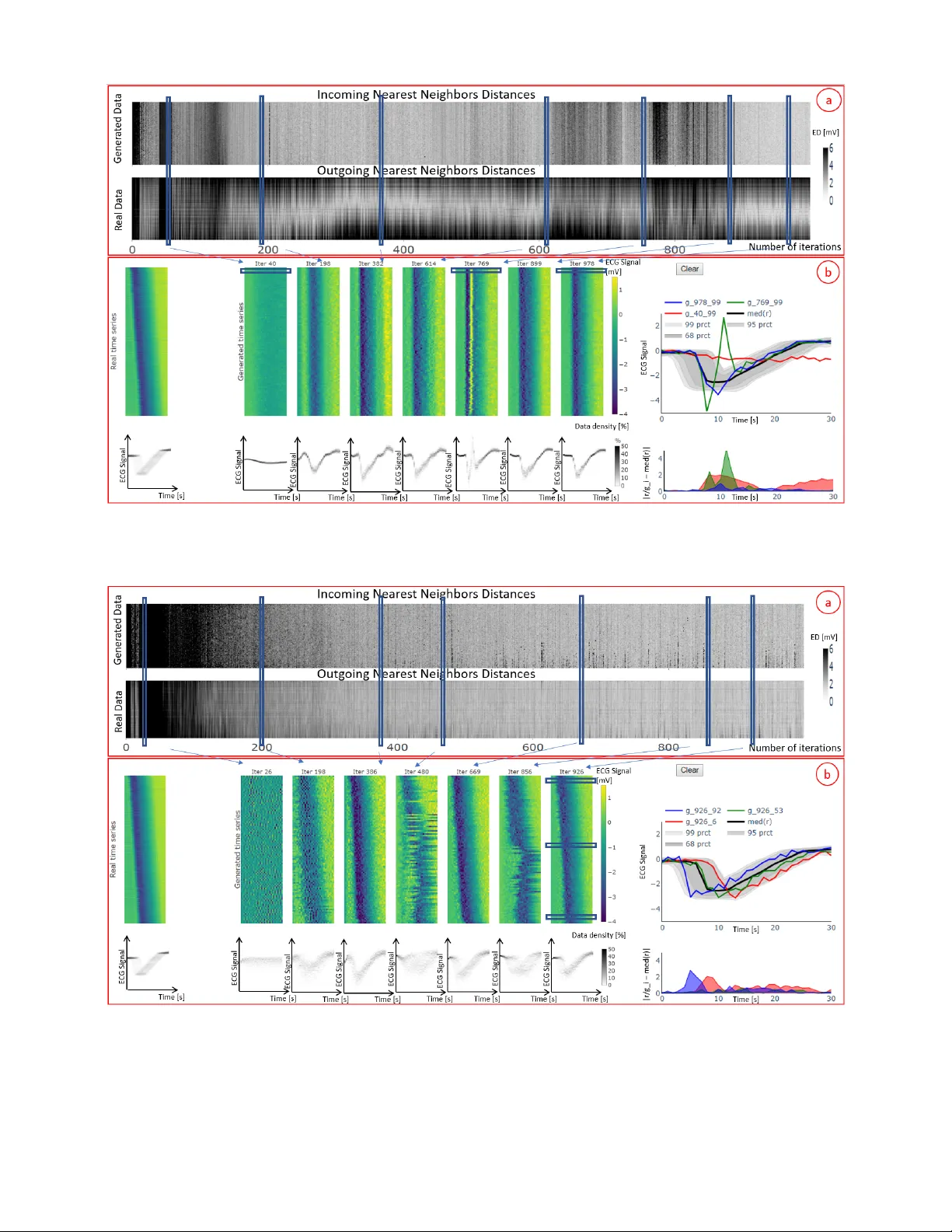
V isual Evaluation of Generati ve Adversarial Networks f or T ime Series Data Hiba Arnout, 1,2 Johannes K ehrer , 1 Johanna Br onner , 1 Thomas Runkler 1,2 1 Siemens A G, Corporate T echnology , Otto-Hahn-Ring 6, 81739 Munich, German y 2 T echnical Uni versity of Munich, Department of Computer Science, Boltzmannstrae 3, 85748 Garching, Germany { hiba.arnout, kehrer .johannes, johanna.bronner , thomas.runkler } @siemens.com Abstract A crucial factor to trust Machine Learning (ML) algorithm decisions is a good representation of its application field by the training dataset. This is particularly true when parts of the training data ha ve been artificially generated to o vercome common training problems such as lack of data or imbalanced dataset. Over the last few years, Generative Adversarial Net- works (GANs) have shown remarkable results in generating realistic data. Howe ver, this ML approach lacks an objecti ve function to ev aluate the quality of the generated data. Numer- ous GAN applications focus on generating image data mostly because they can be easily ev aluated by a human eye. Less ef- forts ha ve been made to generate time series data. Assessing their quality is more complicated, particularly for technical data. In this paper , we propose a human-centered approach supporting a ML or domain expert to accomplish this task using V isual Analytics (V A) techniques. The presented ap- proach consists of two views, namely a GAN Iteration V ie w showing similarity metrics between real and generated data ov er the iterations of the generation process and a Detailed Comparativ e V iew equipped with dif ferent time series visu- alizations such as T imeHistograms, to compare the generated data at dif ferent iteration steps. Starting from the GAN Iter- ation V iew , the user can choose suitable iteration steps for detailed inspection. W e ev aluate our approach with a usage scenario that enabled an efficient comparison of two different GAN models. Introduction T ime-dependent information arises in many fields ranging from meteorology , medicine to stock markets. The analy- sis of such data is a central goal in V A, statistics, or ML and many related approaches e xist (Aigner et al. 2008; Aigner et al. 2011). In particular for ML methods a suf ficient amount of training data and a balanced dataset (i.e. each data class is equally well represented) are crucial for a good per- formance. In reality , ML e xperts often face situations where these criteria are not satisfied. In these cases, generating new data provides a possible solution. This has pushed researchers to in vestigate new methods for data generation. In this context, Generati ve Adversarial Copyright c  2019, Association for the Adv ancement of Artificial Intelligence (www .aaai.org). All rights reserv ed. Networks (GANs) (Goodfello w et al. 2014) are sho wing an outstanding performance. Howe ver , to trust a ML model e.g. a classifier trained on generated data, it is necessary to assess how realistic these data are and hence the performance of the generation process. Most ef forts and best results hav e been shown for image generation, where the quality of the generated data can be easily assessed with the human eye. Some research tried to exploit this technique to generate time series data (Esteban, Hyland, and Rtsch 2017). GAN is a Minimax game between two neural networks i.e. the Generator (G) and the Discriminator (D). D is a bi- nary classifier that tries to maximize its log-likelihood to distinguish between the real and the generated data. At the same time, G is trying to minimize the log-probability of the generated samples that are recognized as false. if the data produced by the generator suf ficiently represent the original data. Much efforts are made by researchers to discover suit- able metrics to ev aluate the performance of GAN and can substitute a human judge. The Discriminator and Genera- tor losses, for example, cannot be considered as a measure of GAN performance and this ML approach lacks an objec- tiv e function that defines an appropriate end of iteration with suitable data quality . V arious ev aluation methods have been described in (Theis, van den Oord, and Bethge 2016) such as Parzen window or Maximum Mean Discrepancy (MMD). As proven in (Theis, van den Oord, and Bethge 2016), the use of these methods has various disadvantages. Other meth- ods e.g. inception score are designed only for images and cannot be easily applied to time series data. Therefore, the quality of the generated data must be visually assessed by a human judge (Esteban, Hyland, and Rtsch 2017). Finding common characteristics and differences between real and generated data may be a complicated and exhausti ve task. In fact, comparing generated datasets to real datasets is a challenge, especially for time series data. In this paper , we propose a V A system to guide the ML expert in this e v aluation process for time series data. The de- veloped framework presents a method that mak e the real and generated data easily comparable by combining V A (Color- field, TimeHistograms) with algorithmic methods and en- able the ML expert to trust the trained GAN model. The contribution of the underlying work consists of an ev alua- tion framework illustrated by two vie ws namely , a GAN It- eration V ie w and a Detailed Comparativ e V ie w , that support ML and domain experts to assess the quality of time series data generated with GAN by providing: • An ov erview visualization that helps the analyst to iden- tify interesting iteration of the GAN generation process. • A comparison interface where the time series are visu- alized in a compact manner and ordered using Principal Components Analysis (PCA) to facilitate comparison by juxtaposition. Related W ork GAN (Goodfellow et al. 2014) has gained a lot of attention in the last fe w years. V arious GAN models hav e been pro- posed such as DCGAN (Radford, Metz, and Chintala 2016). Other GAN models were designed for sequential data (Y u et al. 2017; Mogren 2016; Esteban, Hyland, and Rtsch 2017; Li et al. 2018). Theis et al. (Theis, van den Oord, and Bethge 2016) present an overvie w of different e valuation methods for generative models with a focus on images. These meth- ods can be unreliable and cannot be easily applied to time series data. According to Esteban et al. (Esteban, Hyland, and Rtsch 2017) the ev aluation of GAN is still an important problem. The authors present two ev aluation techniques for GANs generating time series: train on synthetic test on real (TSTR) and train on real test on synthetic (TR TS) where the performance of a model trained on synthetic generated data is evaluated on real data and vice-versa. While their meth- ods are mainly computational, our visual approach permits the user to explore the behavior of GAN ov er the iterations and to select the iteration with the best results. Also, we en- able the user to check that the real data are equally well rep- resented by the generated data which is a general goal for GAN. Recently , different V A tools have been proposed for Deep Learning (DL) models. Hohmann et al. (Hohman et al. 2019) giv e an overvie w about tools developed for interpretability , explainability and debugging purposes or to ease compari- son between different DL models. A V A tool is introduced to understand GAN (Kahng et al. 2019) equipped with two visualizations for D and G to give the user the opportunity to train GAN in the browser and understand its functioning. An approach to understand GAN models and interpret them is presented by W ang et al. (W ang et al. 2018). This method mainly focuses on explaining the behavior of GAN for do- main experts. These approaches did not target the ev aluation of the generated data and the considered GAN models were not designed to generate time series data. Aigner et al. (Aigner et al. 2008) give an extensi ve ov erview of techniques for visualizing and analyzing time series data. Numerous methods were proposed to perform predictiv e analysis on time series (Lu et al. 2017). V an W ijk and V an Selow (V an Wijk and V an Selow 1999) describe an approach to recognize patterns or trends on different time scales. The presented visualization illustrates the average of each cluster of time series equipped with a calendar to high- light the corresponding time scales. Muigg et al. (Muigg et al. 2008) propose a focus+context method to interactiv ely analyze a large number of function graphs. T imeHistograms (K osara, Bendix, and Hauser 2004) are an extended version of the standard histograms that allow a temporal in vestigation. W e utilize this visualization in the Detailed Comparativ e V iew to highlight the time-dependent distribution of the generated data at different iterations and enable the user to check that GAN is capturing the distribu- tion of the real data. Gogolou et al. (Gogolou et al. 2019) compare three visualization methods namely line charts, Horizon graphs and Colorfields in finding and comparing similarities between time series. In this context, multiple time series are compared to a unique time series identified as a query . In our work, we employ Colorfields as a com- pact visualization for comparing many time series at dif fer- ent iterations using juxtaposition. Javed et al. (Jav ed, Mc- Donnel, and Elmqvist 2010) in vestigate the performance of small line graph, braided graph, small multiples and horizon graphs in comparison, slope and discrimination tasks. Ac- cording to this study , shared space techniques fit to a small number of time series, while split space techniques are more suitable for a higher number of time series. Ferstl et al. (Fer - stl et al. 2016) analyze ensembles of iso-contours and use PCA to cluster similar ones. In contrast to their work, we use PCA to sort the time series in a consistent manner such that similar time series are located near each other . Design of Evaluation Framework In this section, we describe our ev aluation framew ork, which supports ML e xperts in generating time series data based on a given number of real data. For the sake of simplicity , we consider uni-variate time series of equal length. In this con- text, we present a workflow that can be used to ev aluate the performance of GAN and assists the ML expert with the data generation. This work is the result of an ongoing collabo- ration between ML and V A experts. The feedback of prac- titioners that use GAN to generate time series helped us in the framework’ s design. Our approach addresses some of the main issues with GAN training that are frequently encoun- tered by ML experts. The V A system fulfills the follo wing design goals: Goal 1 Find iterations where an appropriate behavior is achiev ed i.e. the iterations showing a sufficient quality of the generated data. Check if the number of iterations is sufficient or a higher number of iterations is needed. Goal 2 Compare the performance of different GAN mod- els with different sets of parameters and support the ML expert in the decision making process to either trust or re- ject the current GAN model. Hence, the ML expert should be able to identify which GAN model and subsequently , which set of parameters is better . Goal 3 Present an adequate method to visually e valuate the quality of the generated data i.e. detect if the data are noisy or show a different beha vior compared to the real time series data. ML experts should be able to decide wether the time series generated by a GAN algorithm are realistic. Figure 1: A visual ev aluation workflo w of GANs for time series data: The real and the generated data are integrated in the e valuation frame work. The ML expert may interact with the ev aluation framework to get more insight about the data and their properties. After a rigorous e xploration of the data, he or she can decide to terminate the training process if the desired behavior is achie ved. Otherwise, he or she has to run the GAN model with different parameters. Goal 4 Detect common GAN training problems such as non-con vergence or mode collapse. Mode collapse is an important issue that a ML expert may encounter dur - ing training. In this case, the generator collapses to one mode and is not able to produce div erse samples. Al- most all proposed GAN models (Goodfellow et al. 2014; Radford, Metz, and Chintala 2016) suf fer from this issue. Our purpose is to offer the user the possibility to easily identify this phenomenon. Once the problem is detected, the ML expert can use existing techniques (Salimans et al. 2016) to improve the performance of the considered GAN model. W e design our framew ork based on these criteria. The ML expert starts the process by generating time series with GAN. The ev aluation framework is then used to check whether the GAN model and the generated data fulfill the desired requirements. If this is the case, the ML expert has succeeded to generate realistic data and can stop the gen- eration process. Otherwise he or she will have to rerun the GAN model with different parameters and repeat the inv es- tigations in the frame work. It should be noted that an online ev aluation is also possible, i.e. the framework can be used during the training process. As the training process can take up to se veral days, our approach may help to save valuable time by making sure during the training that the GAN model is going in the right direction or restart the training process if an unexpected behavior is detected. The proposed workflow is depicted in Fig. 1. Evaluation Framework Description Our proposed approach is characterized by two vie ws: a GAN Iteration V ie w that giv es the user a general impression about the behavior of GAN over the iterations of the gen- eration process and a Detailed Comparativ e V iew equipped with TimeHistograms (K osara, Bendix, and Hauser 2004), Colorfields (Gogolou et al. 2019) and line plots to further in vestigate particular time series selected by the user . The T imeHistogram displays the time-dependent distribution of all time series at a certain iteration. At the same time, the Colorfield visualization allows further in vestigation and ex- ploration of a multitude of generated time series at a certain iteration and compares them to the real time series. More- ov er, a direct comparison between specific time series is made possible using the line plots visualization. T o get more insights about the properties of the data, a measure of simi- larity and a dimensionality reduction technique are used: 1. Similarity measures such as Euclidean Distance (ED) or Dynamic T ime W arping (DTW) are used as pairwise dis- tance between two time series. 2. Principal Component Analysis (PCA) is used to arrange similar time series close to each other and facilitate com- parison. GAN Iteration View The vie w consists of two components, namely the incoming and outgoing nearest neighbor distances (see Fig. 2a). The Incoming Nearest Neighbor Distances (INND) represent for each generated time series the minimal distance to a real time series. The user can choose between ED and DTW as a distance measure. The e volution of these minima through- out the iterations is in this case sho wn. W e repeat the same procedure calculating the minima of each real time series to all generated time series. This corresponds to the Outgoing Nearest Neighbor Distances (ONND). A PCA is applied to the real time series data to transform the data points of each time series into uncorrelated components. The real data are then sorted based on the first principal component. T o make both the real and generated data comparable, the same trans- formation is applied to the generated data. A heatmap visu- alization is used to depict the incoming and outgoing mini- mal distances. The intensity of the color of each pixel high- lights the value of the minimal distance. A dark pixel rep- resents a high distance value, while a brighter pixel denotes a lower distance value. The nearest neighbor distances gi ve an o verview about the o verall performance of GAN ov er the iterations and allow for dif ferent types of in vestigations: • Are the time series becoming more realistic with the iter- ations i.e. do the INND/ ONND become smaller? • Are INND / ONND reaching a stable behavior and indi- cating nearly constant values? • Is the variation in the real data representativ e for the generated data i.e. are all types of generated time series equally similar to the real data (INND) and are all real time series equally well represented by the different gen- erated time series or do generated time series correspond to a limited number of real ones (ONND)? The user can interacti vely select interesting iterations in the GAN Iteration V iew and get more insights about the selected iterations in the other view . This will permit him to identify the iteration with the best behavior . For sake of simplicity , we use ED as a similarity measure in the rest of the paper . Detailed Comparative V iew This view is equipped with T imeHistograms (K osara, Bendix, and Hauser 2004) depicting the distribution of the real and the generated data, a Colorfield visualization as a compact representation of the corresponding time series and a Selected Samples V ie w allo wing comparison by superpo- sition (see Fig. 2b). In the Colorfield and TimeHistogram V ie ws, the real data are sho wn on the left and selected itera- tions of the generated data are sho wn on the right. This setup enables a comparison by juxtaposition between the real and the generated data as well as between different iterations of the generation process. The user can inv estigate different it- erations at the same time. Both real and generated data are automatically sorted for each iteration step based on the first principal component. The T imeHistograms enable a time- dependent in vestigation of the distribution of the data and a comparison between the distribution of the real and the generated data. This visualization represents a possibility to check if the model is working properly and capturing the distribution of the real data. The Colorfield visualization is used to depict the time series and enables a rigorous explo- ration of the generated time series and their properties. Each heatmap represents all the data of a specific iteration where each row corresponds to a time series. This visualization per- mits the user to compare a high number of time series in an ef ficient manner . Additionally , a rigorous in vestigation of some selected time series is made possible with the Selected Samples V iew equipped with tw o visualizations. T o gi ve the ML expert more insights about the real data, the first plot de- picts their median med ( r ) and the amount of data falling in the 68 th , 95 th and 99 . 7 th percentile denoted with 68 pr ct , 95 pr ct and 99 prct respectiv ely . The user may add interest- ing, real or generated, time series to the plot to inv estigate their properties and compare them by superposition. Each generated and real time series is denoted with g iter id and r id respectively where iter is the number of the iteration at which the time series was generated and id is the index of the time series sorted with PCA. The second plot highlights the absolute value of the element-wise difference between the selected time series r /g i and the median of the set of real data med ( r ) . This feature provides additional information about the selected data by directly comparing their behavior to a reference v alue, namely the median of the real data. Our main concern is to enable an exploration of the behavior of the ML model ov er the iterations and an in vestigation of the similarity between the real and the generated data. Hence, the presented human-centered approach giv es the opportu- nity to build a relationship of trust between the ML expert and the AI algorithm. Use case T o demonstrate the utility of the dev eloped frame work, our ML expert tested the proposed method on a GAN model (Mogren 2016) to generate data based on the real dataset (Goldberger et al. 2000 June 13). The considered dataset consists of 7 long-term Electrocardiogram (ECG) for a pe- riod of 14 to 22 hours each. It contains two classes depicting the normal and abnormal behavior . T o reduce the training time, only 30 time points from the real time series are con- sidered. The ML e xpert used one class in his experiments. In our case, the performance of GAN is ev aluated for two dif- ferent parameter configurations, namely model 1 and model 2. The corresponding results are depicted in Fig. 2 and 3. The GAN Iteration V iew (Figs. 2a and 3a) depicts the variation of INND and ONND depending on the iterations. The first iterations are characterized by high INND and ONND. As the number of iterations increases, an improv e- ment in terms of INND can be seen. Hence, the generated data are progressiv ely reaching similar values to the original data and the performance of the ML algorithm is increas- ing with a growing number of iterations. Howe ver , the ED values corresponding to some iterations in model 1 sharply increase. Model 2 is sho wing a more stable behavior . In fact, after approximately 300 iterations, the INND are al- most constant. ONND in Fig. 2a show that the values of the ED at the top and bottom of the vie w are still high. As the real time series are sorted with PCA, our expert concludes that the real time series with an important shift are char- acterized by a high outgoing minimal distance. Hence, the time series produced by the first model are similar to a spe- cific type of the real time series namely the time series that are in the middle. He hypothesizes that this GAN model was not able to reproduce the shift present in the real data and is collapsing to one mode. In contrast to model 1, ONND illustrated in Fig. 3a depicts a low outgoing ED for all real data. ONND helped the ML expert to verify that the gener- ated data are diverse and do not correspond to a specific type of time series but to almost all real ones. Afterwards, the ML expert selects some interesting columns in the GAN Iteration V iew and continues his in- vestigation in the other view . For both scenarios, the user selected an iteration at the begin of the training process, certain columns with low EDs in the middle, few columns characterized by high INND and ONND in model 1 and 2 and some columns sho wing a stable behavior within the last hundred iterations. Initially , the time-dependent distribution of the generated data was completely dif ferent from the real data and noise was generated. An improvement in the per- formance is noticeable after approximately 200 iterations. In general, the time-dependent distribution and the quality of the generated data are becoming more realistic o ver the iter - ations. An enhancement in the results is observed between the iterations 382, 614 and 899 for model 1 and the itera- tions 386 and 669 for model 2. T o inspect the behavior of model 1 rigorously , the user selected some time series gen- erated at different iterations. In the Selected Samples V iew , he noticed that at iteration 764 the generated data presents a strange peak and at iteration 40 noise is generated. Hence, the evaluation framework helped the ML expert to detect if the data are noisy or have a different behavior from the real data (Goal 3). T o conclude, GAN was not able to generate realistic time series in the first iterations at all and is learning the proper- ties and features of the real time series ov er the time. How- ev er , the data quality can decrease drastically after one it- eration i.e. iterations 769 and 480 in the first and second scenario respecti vely . The ML expert confirms that this is an expected behavior with neural networks because their per- formance is not monotonic. An inspection of the last hun- dred iterations allows the ML expert to find an iteration with the best result (Goal 1). This corresponds to iteration 978 for model 1 and iteration 926 for model 2. In both cases, the Figure 2: Results of a first GAN model generating time series. The computed incoming and outgoing minimal distances are integrated in the GAN Iteration V ie w (a). Selected columns in the GAN Iteration V iew , denoted with blue rectangles, are depicted in the Detailed Comparativ e V iew (b). Figure 3: Results of a second GAN model obtained by tuning the parameters of the first model. In comparison to model 1, this model is sho wing a more stable and smooth behavior in terms of the incoming and outgoing nearest neighbor distances. The Colorfields, depicted in the Detailed Comparati ve V iew (b), indicate that the last iteration is reproducing the shift present in the real data and its T imeHistogram is similar to the TimeHistogram of the real data. Figure 4: Illustration of the Selected Samples V ie w with the median of the real data med ( r ) , 68 th , 95 th and 99 th per- centile denoted with 68 pr ct , 95 pr ct and 99 pr ct respectiv ely , time series g 926 47 generated at iteration 926 by model 2 and a real time series r 304 . The absolute value of the element-wise differences of g 926 47 and r 304 to the me- dian med ( r ) are denoted in red and blue respecti vely . The time series g 926 47 is falling in the 98 th percentile of the real data and g 926 47 and r 304 are showing a similar be- havior . generated data are smooth and realistic. Ho wev er , the T ime- Histogram of the data generated with model 1 is still differ- ent from the TimeHistogram of the real data. Moreover , the Colorfield V iew demonstrates that the samples are not as di- verse as in the real data. A rigorous inv estigation of these time series in the Selected Samples V ie w shows that all the generated data are falling in the 68th percentile of the real data and are too close to the median i.e. their dif ference to the median of the real data is low . This confirms the hypoth- esis of the ML expert when he observed the GAN Iteration V ie w . Thus, the user was able to easily detect the mode col- lapse phenomenon, one of the hardest training problems for GAN (Goal 4). In order to av oid this problem, the ML expert used in model 2 a normal distributed noise instead of the uni- formly distributed noise and applied a technique introduced in (Salimans et al. 2016) namely mini-batch discrimination. In contrast to model 1, we clearly see that model 2 is repro- ducing the distribution of the real data much better . For fur- ther exploration, the ML expert selected different time series from the Colorfield V ie w and visualize them in the Selected Samples V ie w . He noticed that model 2 is reproducing the shift present in the real data. This model is generating time series that are moved to the right and to the left and are char- acterized, at some data points, with a high dif ference to the median. As a last step, our expert used the Selected Sam- ples V ie w to directly compare the generated and real data. Fig. 4 shows a real and a generated time series selected by the ML expert. W e clearly see that the behavior of the gen- erated time series is similar to the behavior of the real data. Hence, the second GAN model presents a more realistic be- havior and was able at iteration 926 to generate time series that are rare in the real dataset. The ML expert concludes that model 2 is achieving the desired behavior . Hence, the proposed framew ork helped the ML experts to find a trust- worthy GAN model with a set of parameters producing the best results (Goal 2). Finally , the ML expert said that it was helpful to see the ev olution of the behavior of GAN over the iterations and how the similarity between the real and the generated data is improved with the number of iterations. He was able to assess the quality of the generated data and find a reliable GAN model achieving trustw orthy results. Conclusion In this work, we proposed a visual approach to ev aluate and optimize GAN models generating time series data. The proposed method is based on two visualization techniques namely Colorfield and T imeHistogram as well as a dis- tance measure. The distance measure is used in a sophisti- cated manner to compute the incoming and outgoing nearest neighbor distances. The V A system supports ML experts in the e valuation process. The utility of the de veloped frame- work is demonstrated with a real-world use case where the ED is used as a distance measure. In this case, a ML ex- pert evaluated the performance of two dif ferent GAN mod- els in generating time series based on existing real ones. He was able to detect that the first GAN model generates samples which are not div erse. This corresponds to one of two criteria which are verified by the inception score (Bar- ratt and Sharma 2018), a metric to assess the quality of im- ages generated with GAN. The second criteria states that the mapping between the generated and the real data must be clear, i.e. the generated samples should correspond to an easily recognizable class. This aspect will be further consid- ered in a forthcoming publication. Other dev elopments are planned to allow for increased transparency and deeper un- derstanding of the GAN algorithm such as: additional views that highlight the decision making process of the discrimina- tor and an efficient comparison between data generated from different GAN models. Moreover , we plan to consider other GAN architectures and other real-world use cases that will in volve the feedback of different ML and domain experts in a forthcoming publication. The presented work constitutes a starting point to guide a human to decide if data generated by a GAN algorithm can be used to build reliable and trust- worthy Artificial Intelligence (AI) models. W e believ e that this topic will gain in importance in the future since more AI algorithms will rely on generated data. References [Aigner et al. 2008] Aigner, W .; Miksch, S.; Mller, W .; Schumann, H.; and T ominski, C. 2008. V isual methods for analyzing time-oriented data. IEEE T ransactions on V isual- ization and Computer Graphics 14(1):47–60. [Aigner et al. 2011] Aigner , W .; Miksch, S.; Schumann, H.; and T ominski, C. 2011. V isualization of T ime-Oriented Data . Springer Publishing Company , Incorporated, 1st edi- tion. [Barratt and Sharma 2018] Barratt, S., and Sharma, R. 2018. A Note on the Inception Score. arXiv e-prints [Esteban, Hyland, and Rtsch 2017] Esteban, C.; Hyland, S. L.; and Rtsch, G. 2017. Real-valued (medical) time series generation with recurrent conditional gans. In arXiv pr eprint arXiv:1706.02633 . [Ferstl et al. 2016] Ferstl, F .; Kanzler , M.; Rautenhaus, M.; and W estermann, R. 2016. V isual analysis of spatial vari- ability and global correlations in ensembles of iso-contours. Computer Graphics F orum (Pr oc. Eur oV is) 35(3):221–230. [Gogolou et al. 2019] Gogolou, A.; Tsandilas, T .; Palpanas, T .; and Bezerianos, A. 2019. Comparing similarity per- ception in time series visualizations. IEEE T ransactions on V isualization and Computer Graphics 25(1):523–533. [Goldberger et al. 2000 June 13] Goldberger , A. L.; Amaral, L. A. N.; Glass, L.; Hausdorf f, J. M.; Ivano v , P . C.; Mark, R. G.; Mietus, J. E.; Moody , G. B.; Peng, C.- K.; and Stanley , H. E. 2000 (June 13). Phys- ioBank, PhysioT oolkit, and PhysioNet: Components of a new research resource for complex physiologic signals. Cir culation 101(23):e215–e220. Circulation Electronic Pages: http://circ.ahajournals.org/content/101/23/e215.full PMID:1085218; doi: 10.1161/01.CIR.101.23.e215. [Goodfellow et al. 2014] Goodfello w , I.; Pouget-Abadie, J.; Mirza, M.; Xu, B.; W arde-F arley , D.; Ozair , S.; Courville, A.; and Bengio, Y . 2014. Generati ve adversarial nets. In Ghahramani, Z.; W elling, M.; Cortes, C.; Lawrence, N. D.; and W einberger , K. Q., eds., Advances in Neural Informa- tion Pr ocessing Systems 27 . Curran Associates, Inc. 2672– 2680. [Hohman et al. 2019] Hohman, F .; Kahng, M.; Pienta, R.; and Chau, D. H. 2019. V isual analytics in deep learning: An interrogati ve surve y for the next frontiers. IEEE T ransac- tions on V isualization and Computer Graphics 25(8):2674– 2693. [Jav ed, McDonnel, and Elmqvist 2010] Jav ed, W .; McDon- nel, B.; and Elmqvist, N. 2010. Graphical perception of multiple time series. IEEE T ransactions on V isualization and Computer Graphics 16(6):927–934. [Kahng et al. 2019] Kahng, M.; Thorat, N.; Chau, D. H. .; V i- gas, F . B.; and W attenber g, M. 2019. Gan lab: Understand- ing comple x deep generative models using interacti ve visual experimentation. IEEE T ransactions on V isualization and Computer Graphics 25(1):1–11. [K osara, Bendix, and Hauser 2004] K osara, R.; Bendix, F .; and Hauser , H. 2004. Time histograms for large, time- dependent data. In Pr oceedings of the Sixth Joint Eur o- graphics - IEEE TCVG Conference on V isualization , VIS- SYM’04, 45–54. Aire-la-V ille, Switzerland, Switzerland: Eurographics Association. [Li et al. 2018] Li, D.; Chen, D.; Shi, L.; Jin, B.; Goh, J.; and Ng, S. 2018. MAD-GAN: anomaly detection with generativ e adversarial networks for multiv ariate time series. arXiv:1901.04997 [cs.LG]. [Lu et al. 2017] Lu, Y .; Garcia, R.; Hansen, B.; Gleicher , M.; and Macieje wski, R. 2017. The state-of-the-art in predicti ve visual analytics. Comput. Graph. F orum 36:539–562. [Mogren 2016] Mogren, O. 2016. C-rnn-gan: A continuous recurrent neural network with adversarial training. In Con- structive Machine Learning W orkshop (CML) at NIPS 2016 , 1. [Muigg et al. 2008] Muigg, P .; Kehrer , J.; Oeltze-Jafra, S.; Piringer , H.; Doleisch, H.; Preim, B.; and Hauser , H. 2008. A four-le vel focus+context approach to interactiv e visual analysis of temporal features in large scientific data. Com- puter Graphics F orum 27:775–782. [Radford, Metz, and Chintala 2016] Radford, A.; Metz, L.; and Chintala, S. 2016. Unsupervised representation learn- ing with deep conv olutional generative adversarial networks. In International Confer ence on Learning Repr esentations (ICLR) . [Salimans et al. 2016] Salimans, T .; Goodfello w , I.; Zaremba, W .; Cheung, V .; Radford, A.; Chen, X.; and Chen, X. 2016. Improved techniques for training gans. In Lee, D. D.; Sugiyama, M.; Luxbur g, U. V .; Guyon, I.; and Garnett, R., eds., Advances in Neural Information Pr ocessing Systems 29 . Curran Associates, Inc. 2234–2242. [Theis, van den Oord, and Bethge 2016] Theis, L.; van den Oord, A.; and Bethge, M. 2016. A note on the ev aluation of generativ e models. In International Confer ence on Learning Repr esentations , [V an Wijk and V an Selo w 1999] V an W ijk, J. J., and V an Selow, E. R. 1999. Cluster and calendar based visualization of time series data. In Pr oceedings 1999 IEEE Symposium on Information V isualization (InfoV is’99) , 4–9. [W ang et al. 2018] W ang, J.; Gou, L.; Y ang, H.; and Shen, H. 2018. Gan viz: A visual analytics approach to understand the adversarial game. IEEE T ransactions on V isualization and Computer Graphics 24(6):1905–1917. [Y u et al. 2017] Y u, L.; Zhang, W .; W ang, J.; and Y u, Y . 2017. Seqgan: Sequence generativ e adversarial nets with policy gradient. In Pr oceedings of the Thirty-F irst AAAI Confer ence on Artificial Intelligence , AAAI’17, 2852–2858. AAAI Press.