Automatic Scene Inference for 3D Object Compositing

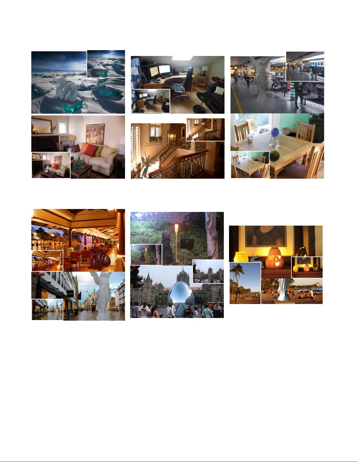
A utomatic Scene Inf erence f or 3D Object Compositing K evin Karsch 1 , Kalyan Sunkav alli 2 , Sunil Hadap 2 , Nathan Carr 2 , Hailin Jin 2 , Rafael F onte 1 , Michael Sittig 1 David F orsyth 1 1 University of Illinois 2 Adobe Research W e present a user-friendly image editing system that supports a drag-and- drop object insertion (where the user merely drags objects into the image, and the system automatically places them in 3D and relights them appro- priately), post-process illumination editing, and depth-of-field manipula- tion. Underlying our system is a fully automatic technique for recovering a comprehensive 3D scene model (geometry , illumination, dif fuse albedo and camera parameters) from a single, low dynamic range photograph. This is made possible by two novel contributions: an illumination inference al- gorithm that recovers a full lighting model of the scene (including light sources that are not directly visible in the photograph), and a depth estima- tion algorithm that combines data-driv en depth transfer with geometric rea- soning about the scene layout. A user study shows that our system produces perceptually convincing results, and achiev es the same level of realism as techniques that require significant user interaction. Categories and Subject Descriptors: I.2.10 [ Computing Methodologies ]: Artificial Intelligence— V ision and Scene Understanding ; I.3.6 [ Comput- ing Methodologies ]: Computer Graphics— Methodology and T echniques Additional Ke y W ords and Phrases: Illumination inference, depth estima- tion, scene reconstruction, physically grounded, image-based rendering, im- age editing 1. INTRODUCTION Many applications require a user to insert 3D characters, props, or other synthetic objects into images. In many existing photo editors, it is the artist’ s job to create photorealistic effects by recognizing the physical space present in an image. For example, to add a new object into an image, the artist must determine how the object will be lit, where shado ws will be cast, and the perspectiv e at which the object will be vie wed. In this paper , we demonstrate a new kind of image editor – one that computes the physical space of the photo- Authors’ email addresses: { karsch1,sittig2,dafonte2,daf } @illinois.edu, { sunkav al,hadap,ncarr,hljin } @adobe.com Permission to make digital or hard copies of part or all of this work for personal or classroom use is granted without fee provided that copies are not made or distributed for profit or commercial advantage and that copies show this notice on the first page or initial screen of a display along with the full citation. Copyrights for components of this work owned by others than A CM must be honored. Abstracting with credit is permitted. T o copy otherwise, to republish, to post on servers, to redistribute to lists, or to use any component of this work in other works requires prior specific permis- sion and /or a fee. Permissions may be requested from Publications Dept., A CM, Inc., 2 Penn Plaza, Suite 701, New Y ork, NY 10121-0701 USA, fax + 1 (212) 869-0481, or permissions@acm.org. c  2009 ACM 0730-0301/2009/20-AR T106 $10.00 DOI 10.1145/1559755.1559763 http://doi.acm.org/10.1145/1559755.1559763 Fig. 1. From a single LDR photograph, our system automatically esti- mates a 3D scene model without any user interaction or additional infor- mation. These scene models facilitate photorealistic, physically grounded image editing operations, which we demonstrate with an intuitiv e interface. W ith our system, a user can simply drag-and-drop 3D models into a picture (top), render objects seamlessly into photographs with a single click (mid- dle), adjust the illumination, and refocus the image in real time (bottom). Best viewed in color at high-resolution. ACM T ransactions on Graphics, V ol. 28, No. 4, Article 106, Publication date: August 2009. 2 • K. Karsch, K. Sunkav alli, S. Hadap , N. Carr , H. Jin, R. F onte, M. Sittig, D . Forsyth Reflectance Depth Rendered 3D scene Final result Intrinsic d ecomposition (Sec 4) Light inference & optimization (Sec 5) Depth inference (Sec 4) Insert & Composite (Sec 6) Input Fig. 2. Our system allows for physically grounded image editing (e.g., the inserted dragon a nd chair on the right), facilitated by our automatic scene estimation procedure. T o compute a scene from a single image, we automatically estimate dense depth and diffuse reflectance (the geometry and materials of our scene). Sources of illumination are then inferred without any user input to form a complete 3D scene, conditioned on the estimated scene geometry . Using a simple, drag-and-drop interface, objects are quickly inserted and composited into the input image with realistic lighting, shadowing, and perspective. Photo credits: c  Salvadonica Bor go. graph automatically , allo wing an artist (or , in fact, anyone) to mak e physically grounded edits with only a fe w mouse clicks. Our system works by inferring the physical scene (geometry , il- lumination, etc.) that corresponds to a single LDR photograph. This process is fully automatic, requires no special hardw are, and works for legacy images. W e show that our inferred scene models can be used to facilitate a variety of physically-based image editing op- erations. For example, objects can be seamlessly inserted into the photograph, light source intensity can be modified, and the picture can be refocused on the fly . Achie ving these edits with existing soft- ware is a painstaking process that takes a great deal of artistry and expertise. In order to facilitate realistic object insertion and rendering we need to hypothesize camera parameters, scene geometry , surface materials, and sources of illumination. T o address this, we de velop a new method for both single-image depth and illumination infer- ence. W e are able to build a full 3D scene model without any user interaction, including camera parameters and reflectance estimates. Contributions. Our primary contribution is a completely automatic algorithm for estimating a full 3D scene model from a single LDR photograph. Our system contains two technical contributions: il- lumination inference and depth estimation. W e have dev eloped a nov el, data-driven illumination estimation procedure that automat- ically estimates a physical lighting model for the entire scene (in- cluding out-of-view light sources). This estimation is aided by our single-image light classifier to detect emitting pixels, which we be- liev e is the first of its kind. W e also demonstrate state-of-the-art depth estimates by combining data-driv en depth inference with ge- ometric reasoning. W e hav e created an intuiti ve interface for inserting 3D mod- els seamlessly into photographs, using our scene approximation method to relight the object and facilitate drag-and-drop inser - tion. Our interface also supports other physically grounded image editing operations, such as post-process depth-of-field and lighting changes. In a user study , we show that our system is capable of making photorealistic edits: in side-by-side comparisons of ground truth photos with photos edited by our softw are, subjects had a dif- ficult time choosing the ground truth. Limitations. Our method works best when scene lighting is dif- fuse, and therefore generally works better indoors than out (see our user studies and results in Sec 7). Our scene models are clearly not canonical representations of the imaged scene and often differ significantly from the true scene components. These coarse scene reconstructions suffice in man y cases to produce realistically edited images. Howev er, in some case, errors in either geometry , illumi- nation, or materials may be stark enough to manifest themselv es in unappealing w ays while editing. For example, inaccurate geometry could cause odd looking shadows for inserted objects, and insert- ing light sources can exacerbate geometric errors. Also, our editing software does not handle object insertion behind existing scene el- ements automatically , and cannot be used to deblur an image taken with wide aperture. A Manhattan W orld is assumed in our camera pose and depth estimation stages, but our method is still applicable in scenes where this assumption does not hold (see Fig 10). 2. RELA TED WORK In order to build a physically based image editor (one that supports operations such as lighting-consistent object insertion, relighting, and ne w vie w synthesis), it is requisite to model the three major factors in image formation: geometry , illumination, and surface re- flectance. Existing approaches are prohibiti ve to most users as the y require either manually recreating or measuring an imaged scene with hardware aids [Debe vec 1998; Y u et al. 1999; Boi vin and Gagalo wicz 2001; Debev ec 2005]. In contrast, Lalonde et al. [2007] and Karsch et al. [2011] have shown that e ven coarse estimates of scene geometry , reflectance properties, illumination, and camera parameters are sufficient for many image editing tasks. Their tech- niques require a user to model the scene geometry and illumination – a task that requires time and an understanding of 3D authoring tools. While our work is similar in spirit to theirs, our technique is fully automatic and is still able to produce results with the same perceptual quality . Similar to our method, Barron and Malik [2013] recover shape, surface albedo and illumination for entire scenes, but their method requires a coarse input depth map (e.g. from a Kinect) and is not di- rectly suitable for object insertion as illumination is only estimated near surfaces (rather than the entire v olume). Geometry . User-guided approaches to single image model- ing [Horry et al. 1997; Criminisi et al. 2000; Oh et al. 2001] have been successfully used to create 3D reconstructions that allow for viewpoint variation. Single image depth estimation techniques ha ve used learned relationships between image features and geometry to estimate depth [Hoiem et al. 2005b; Saxena et al. 2009; Liu et al. 2010; Karsch et al. 2012]. Our depth estimation technique improves upon these methods by incorporating geometric constraints, using intuition from past approaches which estimate depth by assuming a Manhattan W orld ([Delage et al. 2005] for single images, and [Furukawa et al. 2009; Gallup et al. 2010] for multiple images). A CM Transactions on Graphics, V ol. 28, No. 4, Article 106, Publication date: August 2009. A utomatic Scene Inference for 3D Object Compositing • 3 Other approaches to image modeling hav e explicitly parametrized indoor scenes as 3D boxes (or as collections of orthogonal planes) [Lee et al. 2009; Hedau et al. 2009; Karsch et al. 2011; Schwing and Urtasun 2012]. In our work, we use ap- pearance features to infer image depth, but augment this inference with priors based on geometric reasoning about the scene. The contemporaneous works of Satkin et al. [Satkin et al. 2012] and Del Pero et al. [Pero et al. 2013] predict 3D scene reconstruc- tions for the rooms and their furniture. Their predicted models can be very good semantically , but are not suited well for our editing applications as the models are typically not well-aligned with the edges and boundaries in the image. Illumination. Lighting estimation algorithms vary by the represen- tation they use for illumination. Point light sources in the scene can be detected by analyzing silhouettes and shading along ob- ject contours [Johnson and Farid 2005; Lopez-Moreno et al. 2010]. Lalonde et al. [2009] use a physically-based model for sky illu- mination and a data-driv en sunlight model to recover an en viron- ment map from time-lapse sequences. In subsequent work, they use the appearance of the sky in conjunction with cues such as shadows and shading to recover an en vironment map from a sin- gle image [Lalonde et al. 2009]. Nishino et al. [2004] recreate en vironment maps of the scene from reflections in eyes. Johnson and Farid [2007] estimate lower-dimensional spherical harmonics- based lighting models from images. Panagopoulos et al. [2011] show that automatically detected shadows can be used to recov er an illumination en vironment from a single image, but require coarse geometry as input. While all these techniques estimate physically-based lighting from the scene, Khan et al. [2006] sho w that wrapping an image to create the en vironment map can suffice for certain applications. Our illumination estimation technique attempts to predict illu- mination both within and outside the photograph’ s frustum with a data-driv en matching approach; such approaches hav e seen pre vi- ous success in recognizing scene viewpoint [Xiao et al. 2012] and view e xtrapolation [Zhang et al. 2013]. W e also attempt to predict a one-parameter camera response function jointly during our in verse rendering optimization. Other processes exist for recovering camera response, but require multi- ple of images [Diaz and Sturm 2013]. Materials. In order to infer illumination, we separate the input im- age into diffuse albedo and shading using the Color Retinex algo- rithm [Grosse et al. 2009]. W e assume that the scene is Lambertian, and find that this suffices for our applications. Other researchers hav e looked at the problem of recovering the Bi-directional Re- flectance Density Function (BRDF) from a single image, but as far as we know , there are no such methods that work automatically and at the scene (as opposed to object) lev el. These techniques typically make the problem tractable by using lo w-dimensional representations for the BRDF such as spherical harmonics [Ra- mamoorthi and Hanrahan 2004], bi-v ariate models for isotropic reflectances [Romeiro et al. 2008; Romeiro and Zickler 2010], and data-driven statistical models [Lombardi and Nishino 2012a; 2012b]. All these techniques require the shape to be known and in addition, either require the illumination to be giv en, or use priors on lighting to constrain the problem space. Per ception. Even though our estimates of scene geometry , mate- rials, and illumination are coarse, they enable us to create realistic composites. This is possible because e ven lar ge changes in lighting are often not perceivable to the human visual system. This has been shown to be true for both point light sources [Lopez-Moreno et al. 2010] and complex illumination [Ramanarayanan et al. 2007]. 3. METHOD O VER VIEW Our method consists of three primary steps, outlined in Fig 2. First, we estimate the physical space of the scene (camera parameters and geometry), as well as the per-pixel diffuse reflectance (Sec 4). Next, we estimate scene illumination (Sec 5) which is guided by our pre- vious estimates (camera, geometry , reflectance). Finally , our inter- face is used to composite objects, improve illumination estimates, or change the depth-of-field (Sec 6). W e ha ve ev aluated our method with a large-scale user study (Sec 7), and additional details and re- sults can be found in the corresponding supplemental document. Figure 2 illustrates the pipeline of our system. Scene parameterization. Our geometry is in the form of a depth map, which is triangulated to form a polygonal mesh (depth is un- projected according to our estimated pinhole camera). Our illumi- nation model contains polygonal area sources, as well as one or more spherical image-based lights. While unconv entional, our models are suitable for most off-the- shelf rendering softw are, and we hav e found our models to produce better looking estimates than simpler models (e.g. planar geometry with infinitely distant lighting). A utomatic indoor/outdoor scene classification. As a pre- processing step, we automatically detect whether the input image is indoors or outdoors. W e use a simple method: k -nearest-neighbor matching of GIST features [Oli va and T orralba 2001] between the input image and all images from the indoor NYUv2 dataset and the outdoor Make3D Dataset. W e choose k = 7 , and decide use majority-voting to determine if the image is indoors or outdoors (e.g. if 4 of the nearest neighbors are from the Make3D dataset, we consider it to be outdoors). More sophisticated methods could also work. Our method uses dif ferent training images and classifiers de- pending on whether the input image is classified as an indoor or outdoor scene. 4. SINGLE IMAGE RECONSTR UCTION The first step in our algorithm is to estimate the physical space of the scene, which we encode with a depth map, camera parameters, and spatially-varying diffuse materials. Here, we describe how to estimate these components, including a new technique for estimat- ing depth from a single image that adheres to geometric intuition about indoor scenes. Single image depth estimation. Karsch et al. [2012] describe a non-parametric, “depth transfer” approach for estimating dense, per-pix el depth from a single image. While shown to be state-of- the-art, this method is purely data-driven, and incorporates no ex- plicit geometric information present in many photographs. It re- quires a database of RGBD (RGB+depth) images, and transfers depth from the dataset to a nov el input image in a non-parametric fashion using correspondences in appearance. This method has been sho wn to work well both indoors and outdoors; ho wev er , only appearance cues are used (multi-scale SIFT features), and we have good reason to belie ve that adding geometric information will aid in this task. A continuous optimization problem is solved to find the most likely estimate of depth given an input image. In summary , images in the RGBD database are matched to the input and warped so that SIFT features are aligned, and an objectiv e function is minimized to arriv e at a solution. W e denote D as the depth map we wish to infer , and following the notation of Karsch et al., we write the full A CM Transactions on Graphics, V ol. 28, No. 4, Article 106, Publication date: August 2009. 4 • K. Karsch, K. Sunkav alli, S. Hadap , N. Carr , H. Jin, R. F onte, M. Sittig, D . Forsyth Input Orientation hypotheses Edges, VPs, & camera Geometric reasoning RGBD dataset Depth Normals Depth sampling wit h ge ometric constraints Fig. 3. Automatic depth estimation algorithm. Using the geometric rea- soning method of Lee et al. [2009], we estimate focal length and a sparse surface orientation map. Facilitated by a dataset of RGBD images, we then apply a non-parametric depth sampling approach to compute the per-pix el depth of the scene. The geometric cues are used during inference to en- force orientation constraints, piecewise-planarity , and surface smoothness. The result is a dense reconstruction of the scene that is suitable for realistic, physically grounded editing. Photo cr edits: Flickr user c  “Mr .T inDC”. objectiv e here for completeness: argmin D E ( D ) = X i ∈ pixels E t ( D i ) + αE s ( D i ) + β E p ( D i ) , (1) where E t is the data term (depth transfer), E s enforces smoothness, and E p is a prior encouraging depth to look like the average depth in the dataset. W e refer the reader to [Karsch et al. 2012] for details. Our idea is to reformulate the depth transfer objective function and infuse it with geometric information extracted using the ge- ometric reasoning algorithm of Lee et al. [2009]. Lee et al. de- tect vanishing points and lines from a single image, and use these to hypothesize a set of sparse surface orientations for the image. The predicted surface orientations are aligned with one of the three dominant directions in the scene (assuming a Manhattan W orld). W e remove the image-based smoothness ( E s ) and prior terms ( E p ), and replace them with geometric-based priors. W e add terms to enforce a Manhattan W orld ( E m ), constrain the orientation of planar surfaces ( E o ), and impose 3D smoothness ( E 3 s , spatial smoothness in 3D rather than 2D): argmin D E geom ( D ) = X i ∈ pixels E t ( D i ) + λ m E m ( N ( D )) + (2) λ o E o ( N ( D )) + λ 3 s E 3 s ( N ( D )) , where the weights are trained using a coarse-to-fine grid search on held-out ground truth data (indoors: λ m = 100 , λ o = 0 . 5 , λ 3 s = 0 . 1 , outdoors: λ m = 200 , λ o = 10 , λ 3 s = 1 ); these weights dictate the amount of influence each corresponding prior has dur- ing optimization. Descriptions of these priors and implementation details can be found in the supplemental file. Karsch et al. [2012] Our method Normals Input Normals Depth Depth Insertion result Insertion result Fig. 4. Comparison of different depth estimation techniques. Although the depth maps of our technique and of Karsch et al. [2012] appear roughly sim- ilar , the surface orientations provide a sense of ho w distinct the methods are. Our depth estimation procedure (aided by geometric reasoning) is crucial in achieving realistic insertion results, as the noisy surface orientations from Karsch et al. can cause implausible cast shadows and lighting ef fects. Figure 3 shows the pipeline of our depth estimation algorithm, and Fig 4 illustrates the differences between our method and the depth transfer approach; in particular , noisy surface orientations from the depth of Karsch et al. [2012] lead to unrealistic insertion and relighting relights. In supplemental material, we show additional results, including state-of-the-art results on two benchmark datasets using our new depth estimator . Camera parameters. It is well known ho w to compute a simple pinhole camera (focal length, f and camera center, ( c x 0 , c y 0 ) ) and extrinsic parameters from three orthogonal v anishing points [Hart- ley and Zisserman 2003] (computed during depth estimation), and we use this camera model at render-time. Surface materials. W e use Color Retinex (as described in [Grosse et al. 2009]), to estimate a spatially-v arying dif fuse material albedo for each pixel in the visible scene. 5. ESTIMA TING ILLUMINA TION W e categorize luminaires into visible sources (sources visible in the photograph), and out-of-view sources (all other luminaires). V isi- ble sources are detected in the image using a trained “light classi- fier” (Sec 5.1). Out-of-view sources are estimated through a data- driv en procedure (Sec 5.2) using a large dataset of annotated spher - ical panoramas (SUN360 [Xiao et al. 2012]). The resulting lighting A CM Transactions on Graphics, V ol. 28, No. 4, Article 106, Publication date: August 2009. A utomatic Scene Inference for 3D Object Compositing • 5 Light intensity optimization Inferred depth Inferred albedo Input V i s i bl e s ourc e de t e c t i on Out-of-view source estimation Rendered scene (optimized light intensities) 5 light sources; 200 samples per-pixel 12 light sources; 200 samples per-pixel Rendered scene (without intensity optimization) IBL dataset Auto-rank dataset IBLs (compare sampled IBLs and input image features) Choose top k IBLs for relighting Sampled IBLs Fig. 5. Overview of our lighting estimation procedure. Light sources are first detected in the input image using our light classifier . T o estimate light outside of the view frustum, we use a data-driven approach (utilizing the SUN360 panorama dataset). W e train a ranking function to rank IBLs according to ho w well they “match” the input image’ s illumination (see text for details), and use the top k IBLs for relighting. Finally , source intensities are optimized to produce a rendering of the scene that closely matches the input image. Our optimization not only encourages more plausible lighting conditions, but also improves rendering speed by pruning inefficient light sources. model is a hybrid of area sources and spherical emitting sources. Finally , light source intensities are estimated using an optimization procedure which adjusts light intensities so that the rendered scene appears similar to the input image (Sec 5.3). Figure 5 illustrates this procedure. Dataset. W e have annotated light sources in 100 indoor and 100 outdoor scenes from the SUN360 dataset. The annotations also in- clude a discrete estimate of distance from the camera (“close”: 1- 5m, “medium”: 5-50m, “far”: > 50m, “infinite”: reserved for sun). Since SUN360 images are LDR and tonemapped, we make no at- tempt to annotate absolute intensity , only the position/direction of sources. Furthermore, the goal of our classifier is only to predict location (not intensity). This data is used in both our in-view and out-of-view techniques belo w . 5.1 Illumination visible in the view frustum T o detect sources of light in the image, we hav e dev eloped a new light classifier . For a given image, we segment the image into su- perpixels using SLIC [Achanta et al. 2012], and compute features for each superpixel. W e use the following features: the height of the superpixel in the image (obtained by averaging the 2D loca- tion of all pixels in the superpixel), as well as the features used by Make3D 1 [Saxena et al. 2009]. Using our annotated training data, we train a binary classifier to predict whether or not a superpixel is emitting/reflecting a sig- 1 17 edge/smoothing filter responses in YCbCr space are averaged over the superpixel. Both the energy and kurtosis of the filter responses are com- puted (second and fourth powers) for a total of 34 features, and then con- catenated with four neighboring (top,left,bottom,right) superpixel features. This is done at tw o scales (50% and 100%), resulting in 340(= 34 × 5 × 2 ) features per superpixel. nificant amount of light using these features. For this task, we do not use the discrete distance annotations (these are ho wev er used in Sec 5.2). A classification result is shown in Figure 5. In supple- mental material, we sho w many more qualitative and quantitativ e results of our classifier, and demonstrate that our classifier signifi- cantly outperforms baseline detectors (namely thresholding). For each detected source superpixel (and corresponding pixels), we find their 3D position using the pixel’ s estimated depth and the projection operator K . Writing D as the estimated depth map and ( x, y ) as a pixel’ s position in the image plane, the 3D position of the pixel is gi ven by: X = D ( x, y ) K − 1 [ x, y , 1] T , (3) where K is the intrinsic camera parameters (projection matrix) ob- tained in Section 4. W e obtain a polygonal representation of each light source by fitting a 3D quadrilateral to each cluster (oriented in the direction of least v ariance). Notice that this only provides the position of the visible light sources; we describe how we estimate intensity in Section 5.3. Figure 5 (top) shows a result of our light detector . One might wonder why we train using equirectangular images and test using rectilinear images. Dror et al. [2004] showed that many image statistics computed on equirectangular images follow the same distributions as those computed on rectilinear images; thus features computed in either domain should be roughly the same. W e have also tested our method on both kinds of images (more results in the supplemental file), and see no noticeable dif- ferences. 5.2 Illumination outside of the view frustum Estimating lighting from behind the camera is arguably the most difficult task in single-image illumination estimation. W e use a data-driv en approach, utilizing the extensiv e SUN360 panorama A CM Transactions on Graphics, V ol. 28, No. 4, Article 106, Publication date: August 2009. 6 • K. Karsch, K. Sunkav alli, S. Hadap , N. Carr , H. Jin, R. F onte, M. Sittig, D . Forsyth dataset of Xiao et al. [2012]. Ho wever , since this dataset is not av ailable in HDR, we hav e annotated the dataset to include light source positions and distances. Our primary assumption is that if two photographs hav e simi- lar appearance, then the illumination environment be yond the pho- tographed region will be similar as well. There is some empirical evidence that this can be true (e.g. recent image-extrapolation meth- ods [Zhang et al. 2013]), and studies suggest that people hallucinate out-of-frame image data by combining photographic evidence with recent memories [Intraub and Richardson 1989]. Using this intuition, we develop a nov el procedure for match- ing images to luminaire-annotated panoramas in order to predict out-of-view illumination. W e sample each IBL into N rectilinear projections (2D) at different points on the sphere and at varying fields-of-view , and match these projections to the input image us- ing a variety of features described below (in our work, N = 10 stratified random samples on the sphere with azimuth ∈ [0 , 2 π ) , el- ev ation ∈ [ − π 6 , π 6 ] , FO V ∈ [ π 3 , π 2 ] ). See the bottom of Fig 5 for an illustration. These projections represent the images a camera with that certain orientation and field of view would have captured for that particular scene. By matching the input image to these projec- tions, we can effecti vely ”extrapolate” the scene outside the field of view and estimate the out-of-vie w illumination. Giv en an input image, our goal is to find IBLs in our dataset that emulate the input’ s illumination. Our rectilinear sampled IBLs pro- vide us with ground truth data for training: for each sampled image, we know the corresponding illumination. Based on the past success of rank prediction for data-dri ven geometry estimation [Satkin et al. 2012], we use this data and train an IBL rank predictor (for an input image, rank the dataset IBLs from best to worst). Featur es. After sampling the panoramas into rectilinear images, we compute seven features for each image: geometric context [Hoiem et al. 2005a], orientation maps [Lee et al. 2009], spatial pyra- mids [Lazebnik et al. 2006], HSV histograms (three features total), and the output of our light classifier (Sec 5.1). W e are interested in ranking pairs of images, so our final feature describes ho w well two particular images match in feature space. The result is a 7-dimensional vector where each component de- scribes the similarity of a particular feature (normalized to [0,1], where higher values indicate higher similarity). Similarity is mea- sured using the histogram intersection score for histogram features (spatial pyramid – sp – and HSV – h,s,v – histograms), and follo w- ing Satkin et al. [2012], a normalized, per-pix el dot product (av- eraged over the image) is used for for other features (geometric contact – gc, orientation maps – om, light classifier – lc). More formally , let F i , F j be the features computed on images i and j , and x i j be the vector that measures similarity between the features/images: x i j = [ nd ( F gc i , F gc j ) , nd ( F om i , F om j ) , nd ( F lc i , F lc j ) , hi ( F sp i , F sp j ) , hi ( F h i , F h j ) , hi ( F s i , F s j ) , hi ( F v i , F v j )] T , (4) where nd ( · ) , hi ( · ) are normalized dot product and histogram in- tersection operators respectively . In order to compute per-pix el dot products, images must be the same size. T o compute features on two images with unequal dimension, we downsample the lar ger im- age to hav e the same dimension as the smaller image. T raining loss metric. In order to discriminate between different IBLs, we need to define a distance metric that measure how similar one IBL is to another . W e use this distance metric as the loss for our rank training optimization where it encodes the additional margin when learning the ranking function (Eq 6). A na ¨ ıve way to measure the similarity between two IBLs is to use pixel-wise or template matching [Xiao et al. 2012]. Howev er, this is not ideal for our purposes since it requires accurate correspon- dences between elements of the scene that may not be important from a relighting aspect. Since our primary goal is re-rendering, we define our metric on that basis of ho w different a set of canonical objects appear when they are illuminated by these IBLs. In partic- ular , we render nine objects with v arying materials (dif fuse, glossy , metal, etc.) into each IBL en vironment (see supplemental material). Then, we define the distance as the mean L2 error between the ren- derings. One ca veat is that our IBL dataset isn’t HDR, and we don’t know the intensities of the annotated sources. So, we compute er- ror as the minimum over all possible light intensities. Define I i and I j as two IBLs in our dataset, and I i = [ I (1) i , . . . , I ( n ) i ] , I j = [ I (1) j , . . . , I ( m ) j ] as column-vectorized images rendered by the IBLs for each of the IBLs’ sources (here I i has n sources, and I j has m ). Since a change in the intensity of the IBL corresponds to a change of a scale factor for the rendered image, we define the distance as the minimum rendered error ov er all possible intensities ( y i and y j ): d ( I i , I j ) = min y i ,y j || I i y i − I j y j || , s.t. || [ y T i , y T j ] || = 1 . (5) The constraint is employed to avoid the trivial solution, and we solve this using SVD. T raining the ranking function. Our goal is to train a ranking func- tion that can properly rank images (and their corresponding IBLs) by ho w well their features match the input’ s. Let w be a linear rank- ing function, and x i j be features computed between images i and j . Giv en an input image i and an y two images from our dataset (sam- pled from the panoramas) j and k , we wish to find w such that w T x i j > w T x i k when the illumination of j matches the illumina- tion of i better than the illumination of k . T o solve this problem, we perform a standard 1-slack, linear SVM-ranking optimization [Joachims 2006]: argmin w,ξ || w || 2 + C ξ , s.t. w T x i j ≥ w T x i k + δ i j,k − ξ , ξ ≥ 0 , (6) where x are pairwise image similarity features (Eq 4), and δ i j,k = max( d ( I i , I k ) − d ( I i , I j ) , 0) is a hinge loss to encourage additional margin for examples with unequal distances (according to Eq 5, where I i is the IBL corresponding to image i ). Inference. T o predict the illumination of a nov el input image ( i ), we compute the similarity feature vector (Eq 4) for all input- training image pairs ( x i j , ∀ j ), and sort the prediction function re- sponses ( w T x i j ) in decreasing order . Then, we use choose the top k IBLs (in our work, we use k = 1 for indoor images, and k = 3 outdoors to improve the odds of predicting the correct sun loca- tion). Figure 5 (bottom) shows one indoor result using our method (where k = 2 for demonstration). 5.3 Intensity estimation through render ing Having estimated the location of light sources within and outside the image, we must now recover the relativ e intensities of the sources. Given the exact geometry and material of the scene (in- cluding light source positions), we can estimate the intensities of the sources by adjusting them them until a rendered version of the scene matches the original image. While we do not kno w exact ge- ometry/materials, we assume that our automatic estimates are good enough, and could apply the abo ve rendering-based optimization to A CM Transactions on Graphics, V ol. 28, No. 4, Article 106, Publication date: August 2009. A utomatic Scene Inference for 3D Object Compositing • 7 recov er the light source intensities; Fig 5 shows this process. Our optimization has two goals: match the rendered image to the input, and differing from past techniques [Boi vin and Gagalowicz 2001; Karsch et al. 2011], ensure the scene renders efficiently . Define L i as the intensity of the i th light source, I as the in- put image, and R ( · ) as a scene “rendering” function that takes a set of light intensities and produces an image of the scene illu- minated by those lights (i.e., R ( L ) ). W e want to find the inten- sity of each light source by matching the input and rendered im- ages, so we could solve argmin L P i ∈ pixels || I i − R i ( L ) || . How- ev er, this optimization can be grossly inefficient and unstable, as it requires a new image to be rendered for each function ev alua- tion, and rendering in general is non-differentiable. Howe ver , we can use the fact that light is additive, and write R ( · ) as a linear combination of “basis” renders [Schoeneman et al. 1993; Nimeroff et al. 1994]. W e render the scene (using our estimated geometry and diffuse materials) using only one light source at a time (i.e., L k = 1 , L j = 0 ∀ j 6 = k , implying L = e k ). This results in one rendered image per light source, and we can write a new render function as R 0 ( w ) = C ( P k w k R ( e k )) , where C is the camera re- sponse function, and R ( e i ) is the scene rendered with only the i th source. In our work, we assume the camera response can be mod- eled as an exponent, i.e., C ( x ) = x γ . This allows us to rewrite the matching term abov e as Q ( w, γ ) = X i ∈ pixels           I i − " X k ∈ sources w k R i ( e k ) # γ           . (7) Since each basis render , R ( e k ) , can be precomputed prior to the op- timization, Q can be minimized more ef ficiently than the originally described optimization. W e have hypothesized a number of light source locations in Secs 5.1 and 5.2, and because our scene materials are purely dif- fuse, and our geometry consists of a small set of surface normals, there may exist an infinite number of lighting configurations that produce the same rendered image. Interestingly , user studies hav e shown that humans cannot distinguish between a range of illumi- nation configurations [Ramanarayanan et al. 2007], suggesting that there is a family of lighting conditions that produce the same per- ceptual response. This is actually advantageous, because it allows our optimization to choose only a small number of “good” light sources and prune the rest. In particular, since our final goal is to relight the scene with the estimated illumination, we are interested in lighting configurations that can be rendered faster . W e can easily detect if a particular light source will cause long render times by rendering the image with the given source for a fixed amount of time, and checking the variance in the rendered image (i.e., noise); we incorporate this into our optimization. By rendering with fewer sources and sources that contribute less variance, the scenes pro- duced by our method render significantly faster than without this optimization (see Fig 5, right). Specifically , we ensure that only a small number of sources are used in the final lighting solution, and also prune problematic light sources that may cause inefficient rendering. W e encode this with a sparsity prior on the source intensities and a smoothness prior on the rendered images: P ( w ) = X k ∈ sources   || w k || 1 + w k X i ∈ pixels ||∇ R i ( e k ) ||   . (8) Intuitiv ely , the first term coerces only a small number of nonzero elements in w , and the second term discourages noisy basis ren- ders from having high weights (noise in a basis render typically indicates an implausible lighting configuration, making the giv en image render much more slowly). Combining the previous equations, we de velop the follo wing op- timization problem: argmin w,γ Q ( w, γ ) + λ P P ( w ) + λ γ || γ − γ 0 || , s.t. w k ≥ 0 ∀ k , γ > 0 , (9) where λ P = λ γ = 0 . 1 are weights, and γ 0 = 1 2 . 2 . W e use a con- tinuous approximation to the absolute value ( | x | ≈ √ x 2 +  ), and solve using the activ e set algorithm [Nocedal and Wright 2006]. The computed weights ( w ) can be directly translated into light in- tensities ( L ), and we no w hav e an entire model of the scene (ge- ometry , camera, and materials from Sec 4, and light source posi- tions/intensities as described abov e). Our method has sev eral advantages to past “optimization- through-rendering” techniques [Karsch et al. 2011]. First, our tech- nique has the ability to discard unnecessary and inefficient light sources by adding illumination priors (Eq 8). Second, we esti- mate the camera response function jointly during our optimization, which we do not believ e has been done pre viously . Finally , by solv- ing for a simple linear combination of pre-rendered images, our optimization procedure is much faster than previous methods that render the image for each function e valuation (e.g., as in [Karsch et al. 2011]). Furthermore, our basis lights could be refined or op- timized with user-dri ven techniques guided by aesthetic principles (e.g. [Boyadzhie v et al. 2013]). 6. PHYSICALL Y GROUNDED IMAGE EDITING One of the potential applications of our automatically generated 3D scene models is physically grounded photo editing. In other w ords, we can use the approximate scene models to facilitate physically- based image edits. For e xample, one can use the 3D scene to insert and composite objects with realistic lighting into a photograph, or ev en adjust the depth-of-field and aperture as a post-process. There are many possible interactions that become av ailable with our scene model, and we have developed a prototype interface to facilitate a fe w of these. Realistically inserting synthetic objects into legac y photographs is our primary focus, but our application also allows for post-process lighting and depth-of-field changes. T o fully leverage our scene models, we require physically based rendering software. W e use LuxRender 2 , and hav e built our appli- cation on top of LuxRender’ s existing interface. Figure 6 illustrates the possible uses of the interface, and we refer the reader to the accompanying video for a full demonstration. Drag-and-drop insertion. Once a user specifies an input image for editing, our application automatically computes the 3D scene as described in sections 4 and 5. Based on the inserted location, we also add additional geometric constraints so that the depth is flat in a small region region around the base of the inserted object. For a giv en image of size 1024 × 768 , our method takes approx- imately five minutes on a 2.8Ghz dual core laptop to estimate the 3D scene model, including depth and illumination (this can also be precomputed or computed remotely for efficiency , and only occurs once per image). Next, a user specifies a 3D model and places it in the scene by simply clicking and dragging in the picture (as in Fig 1). Our scene reconstruction facilitates this insertion: our esti- mated perspecti ve camera ensures that the object is scaled properly 2 http://www.luxrender.net A CM Transactions on Graphics, V ol. 28, No. 4, Article 106, Publication date: August 2009. 8 • K. Karsch, K. Sunkav alli, S. Hadap , N. Carr , H. Jin, R. F onte, M. Sittig, D . Forsyth (a) (b) (c) (d) (e) (f) Fig. 6. Our user interface provides a drag-and-drop mechanism for inserting 3D models into an image (input image overlaid on our initial result). Our system also allows for real-time illumination changes without re-rendering. Using simple slider controls, shadows and interreflections can be softened or hardened (a,b), light intensity can be adjusted to achiev e a dif ferent mood (c,d), and synthetic depth-of-field can be applied to re-focus the image (e,f). See the accompanying video for a full demonstration. Best viewed in color at high-resolution. Photo credits: c  Rachel T itiriga (top) and Flickr user c  “Mr .T inDC” (bottom). as it mov es closer/farther from the camera, and based on the sur- face orientation of the clicked location, the application automati- cally re-orients the inserted model so that its up vector is aligned with the surface normal. Rigid transformations are also possible through mouse and keyboard input (scroll to scale, right-click to rotate, etc). Once the user is satisfied with the object placement, the object is rendered into the image 3 . W e use the additiv e differential render- ing method [Debev ec 1998] to composite the rendered object into the photograph, but other methods for one-shot rendering could be used (e.g. Zang et al. [2012]). This method renders tw o images: one containing synthetic objects I obj , and one without synthetic objects I noobj , as well as an object mask M (scalar image that is 0 every- where where no object is present, and (0, 1] otherwise). The final composite image I f inal is obtained by I f inal = M  I obj + (1 − M )  ( I b + I obj − I noobj ) , (10) where I b is the input image, and  is the entry-wise product. For efficienc y (less v ariance and ov erhead), we have implemented this equation as a surface integrator plugin for LuxRender . Specifically , we modify LuxRender’ s bidirectional path tracing implementa- tion [Pharr and Humphreys 2010] so that pixels in I f inal are intel- ligently sampled from either the input image or the rendered scene such that inserted objects and their lighting contributions are ren- dered seamlessly into the photograph. W e set the maximum number of eye and light bounces to 16, and use LuxRender’ s default Rus- sian Roulette strate gy (dynamic thresholds based on past samples). 3 Rendering time is clearly dependent on a number of factors (image size, spatial hierarchy , inserted materials, etc), and is slowed by the fact that we use an unbiased ray-tracer . The results in this paper took between 5 minutes and several hours to render , but this could be sped up depending on the application and resources av ailable. The user is completely abstracted from the compositing process, and only sees I f inal as the object is being rendered. The above insertion method also works for adding light sources (for example, inserting and emitting object). Figure 1 demonstrates a drag-and- drop result. Lighting adjustments. Because we ha ve estimated sources for the scene, we can modify the intensity of these sources to either add or subtract light from the image. Consider the compositing process (Eq 10 with no inserted objects; that is, I obj = I noobj , implying I f inal = I b . Now , imagine that the intensity of a light source in I obj is increased (but the corresponding light source in I noobj re- mains the same). I obj will then be brighter than I noobj , and the compositing equation will reflect a physical change in brightness (effecti vely rendering a more intense light into the scene). Simi- larly , decreasing the intensity of source(s) in I obj will remov e light from the image. Notice that this is a physical change to the lighting in the picture rather than tonal adjustments (e.g., applying a func- tion to an entire image). This technique works similarly when there are inserted objects present in the scene, and a user can also manually adjust the light intensities in a scene to achie ve a desired ef fect (Fig 6, top). Rather than just adjusting source intensities in I obj , if sources in both I obj and I noobj are modified equally , then only the intensity of the in- serted object and its interreflections (shado ws, caustics, etc) will be changed (i.e. without adding or removing light from the rest of the scene). By keeping track of the contribution of each light source to the scene, we only need to render the scene once, and lighting ad- justments can be made in real time without re-rendering (similar to [Loscos et al. 1999; Gibson and Murta 2000]). Figure 6 shows post-process lighting changes; more can be found in supplemental material. A CM Transactions on Graphics, V ol. 28, No. 4, Article 106, Publication date: August 2009. A utomatic Scene Inference for 3D Object Compositing • 9 Synthetic depth-of-field. Our prototype also supports post- focusing the input image: the user specifies a depth-of-field and an aperture size, and the image is adapti vely blurred using our pre- dicted depth map ( D ). Write I f inal as the composite image with in- serted objects (or the input image if nothing is inserted), and G ( σ ) as a Gaussian kernel with standard deviation σ . W e compute the blur at the i th pixel as I dof ,i = I f inal,i ? G ( a | D i − d | ) , (11) where d is the depth of field, and a corresponds to the aperture size. Figures 1 and 6 (bottom) shows a post-focus result. 7. EV ALU A TION W e conducted two user studies to ev aluate the “realism” achiev ed by our insertion technique. Each user study is a series of two- alternativ e forced choice tests, where the subject chooses between a pair of images which he/she feels looks the most realistic. In the first study (Sec 7.1), we use real pictures. Each pair of images contains one actual photograph with a small object placed in the scene, and the other is photo showing a similar object inserted synthetically into the scene (without the actual object present). The second study (Sec 7.2) is v ery similar , but we use highly re- alistic, synthetic images rather than real pictures. For one image, a synthetic object is placed into the full 3D en vironment and ren- dered (using unbiased, physically-based ray tracing); in the other, the same 3D scene is rendered without the synthetic object (using the same rendering method), and then synthetically inserted into the photograph (rather than the 3D scene) using our method. Finally , we visualize the quantitativ e accuracy achieved by our estimates in Section 7.3. 7.1 Real image user study Experimental setup. W e recruited 30 subjects for this study , and we used a total of 10 synthetic objects across three unique, real scenes. Each subject saw each inserted object only once, and viewed sev en to nine side-by-side trial images; one was a real pho- tograph containing a real object, and the other is a synthetic image produced by our method (containing a synthetic version of the real object in the real photo). Subjects were asked to choose the image they felt looked most realistic. T rials and conditions were permuted to ensure ev en coverage. An example trial pair is shown in Fig 7, and more can be found in supplemental material. Conditions. W e tested six binary conditions that we hypothesized may contribute to a subject’ s performance: expert subject; realis- tic shape ; complex material ; automatic result; multiple objects inserted; and whether the trial occured in the first half of a sub- ject’ s study (to test whether there was any learning ef fect present). Subjects were deemed experts if they had graphics/vision experi- ence (in the study , this meant graduate students and researchers at a company lab), and non-experts otherwise. The authors classified objects into realistic/synthetic shape and complex/simple material beforehand. W e created results with our automatic drag-and-drop procedure as one condition (“automatic”), and using our interface, created an improv ed (as judged by the authors) version of each re- sult by manually adjusting the light intensities (“refined”). Results. On average, the result generated by our automatic method was selected as the real image in 34.1% of the 232 pairs that subjects viewed. The refined condition achieved 35.8% confusion, howe ver these distributions do not significantly differ using a two- tailed t-test. An optimal result would be 50%. For comparison, A1 A2 B1 B2 Fig. 7. Example trials from our “real image” user study (top) and our “synthetic image” user study (bottom). In the studies, users were shown two side-by-side pictures; one photograph is real (or rendered photorealistically with an exact 3D scene), and the other has syn- thetic objects inserted into it with our method. Users were instructed to choose the picture from the pair that looked the most realistic. For each ro w , which of the pair would you choose? Best vie wed in color at high-resolution. Scene modeling credits (bottom): Matthew Harwood. A1,B2: r eal/fully render ed; A2, B1: cr eated with our method Karsch et al. [2011] ev aluated their semiautomatic method with a similar user study , and achieved 34% confusion, although their study (scenes, subjects, etc) were not identical to ours. W e also tested to see if any of the other conditions (or combi- nation of conditions) were good predictors of a person’ s ability to perform this task. W e first used logistic regression to predict which judgements would be correct using the features, followed by a Lasso ( L 1 regularized logistic re gression [T ibshirani 1996], in the Matlab R2012b implementation) to identify features that predicted whether the subject judged a particular pair correctly . W e e valuated deviance (mean negati ve log-likelihood on held out data) with 10- fold cross validation. The lowest deviance regression ignores all features; incorporating the “expert” and “realistic shape” features causes about a 1% increase in the deviance; incorporating other features causes the deviance to increase somewhat. This strongly suggests that none of the features actually affect performance. 7.2 Synthetic image user study Our “real image” study pro vides encouraging initial results, but it is limited due to the nature of data collection. Collecting correspond- ing real and synthetic objects with high-quality geometry and re- flectance properties can be extremely dif ficult, so we confined our real image study to small, tabletop accessories (household items and 3D-printable items). In this follow-up study , we utilize highly realistic, synthetic 3D scenes in order to more extensively ev aluate our method (objects with larger -pixel cov erage and varying materials/geometry , div erse lighting conditions, indoors/outdoors). Experimental setup. W e collected four synthetic (yet highly real- istic 4 ) scenes – three indoor, one outdoor . For each scene, we in- 4 W e pre qualified these images as highly-confusable with real pictures in a preliminary study; see supplemental material. A CM Transactions on Graphics, V ol. 28, No. 4, Article 106, Publication date: August 2009. 10 • K. Karsch, K. Sunkav alli, S. Hadap , N. Carr , H. Jin, R. F onte, M. Sittig, D . Forsyth serted three realistic 3D models using con ventional modeling soft- ware (Blender, http://www.blender.org/ ), and rendered each scene using LuxRender under three lighting conditions (v arying from strongly directed to dif fuse light), for a total of 36 (= 4 scenes × 3 objects × 3 lighting conditions) unique and v aried scenes (view able in supplemental material). Next, we used our method to insert the same 3D models in roughly the same location into the empty , rendered images, resulting in 36 “synthetic” insertion re- sults corresponding to the 36 ground truth rendered images. For the study , each participant vie wed 12 pairs 5 of corresponding images, and was asked to select which image he/she felt looked the most realistic (two-alternati ve forced choice). For example, a subject might see two identical bedroom scenes with a ceiling fan, except in one picture, the fan had actually been inserted using our method (see Fig 7). W e polled 450 subjects using Mechanical Turk. In an attempt to av oid inattentiv e subjects, each study also included four “qualifi- cation” image pairs (a cartoon picture next to a real image) placed throughout the study in a stratified fashion. Subjects who incor- rectly chose any of the four cartoon picture as realistic were re- mov ed from our findings (16 in total, leaving 434 studies with us- able data). At the end of the study , we showed subjects two additional image pairs: a pair containing rendered spheres (one a physically plausi- ble, the other not), and a pair containing line drawings of a scene (one with proper vanishing point perspectiv e, the other not). For each pair, subjects chose the image they felt looked most realistic. Then, each subject completed a brief questionnaire, listing demo- graphics, expertise, and v oluntary comments. Methods tested. W e are primarily interested in determining how well our method compares to the ground truth images, b ut also test other illumination estimation methods as baselines. W e generate re- sults using the method of Khan et al. [2006] (projecting the input image onto a hemisphere, duplicating it, and using this as the illu- mination en vironment), the method of Lalonde et al. [2009] (for outdoor images only), and a simplified IBL-matching technique that finds a similar IBL to the input image by template matching (similar to [Xiao et al. 2012]; we use this method indoors only). For each method, only the illumination estimation stage of our pipeline changes (depth, reflectance, and camera estimation remain the same), and all methods utilize our lighting optimization tech- nique to estimate source intensity (Sec 5.3). Conditions. Because we found no condition in our initial study to be a useful predictor of people’ s ability to choose the real image, we introduce many ne w (and perhaps more telling) conditions in this study: indoor/outdoor scene, diffuse/direct lighting in the scene, simple/complex material of inserted object, good/poor composi- tion of inserted object, and if the inserted object has good/poor perspective . W e also assigned each subject a set of binary condi- tions: male/female , age < 25 / ≥ 25 , color-normal / not color - normal , whether or not the subject correctly identified both the physically accurate sphere and the proper-perspecti ve line dra wing at the end of the study ( passed/failed perspective-shading (p-s) tests ), and also expert/non-expert (subjects were classified as ex- perts only if the y passed the perspectiv e-shading tests and indicated that they had e xpertise in art/graphics). Results and discussion. Overall, our synthetic image study sho wed that people confused our insertion result with the true rendered im- 5 Image pairs are randomly permuted/selected so that each of the 12 objects appears exactly once to each subject. T able I. Fraction of times subjects chose a synthetic insertion result ov er the ground truth insertion in our user study Condition N ours Khan Lalonde/matching indoor 1332 .377 .311 .279 outdoor 444 .288 .297 .240 diffuse light 1184 .377 .332 .238 directional light 592 .311 .257 .330 simple material 1036 .353 .301 .248 complex material 740 .357 .315 .299 large co verage 1332 .355 .324 .277 small coverage 444 .356 .253 .245 good composition 1036 .356 .312 .265 poor composition 740 .353 .300 .274 good perspectiv e 1036 .378 .316 .287 poor perspectiv e 740 .322 .295 .244 male 1032 .346 .295 .267 female 744 .367 .319 .272 age ( ≤ 25) 468 .331 .294 .234 age ( > 25) 1164 .363 .312 .284 color normal 1764 .353 .308 .267 not color normal 12 .583 .167 .361 passed p-s tests 1608 .341 .297 .260 failed p-s tests 168 .482 .500 .351 non-expert 1392 .361 .312 .275 expert 384 .333 .288 .252 overall 1776 .355 .307 .269 Highlighted blocks indicate that there are significant differences in confusion when a particular condition is on/off ( p value < 0 . 05 using a 2-tailed t-test). For exam- ple, in the top left cell, the “ours indoor” distribution was found to be significantly different from the “ours outdoor” distribution. For the Lalonde/matching column, the method Lalonde et al. is used for outdoor images, and the template matching technique is used indoors (see text for details). The best method for each condition is sho wn in bold. N is the total number of samples. Overall, our confusion rate of 35.5% better than the baselines (30.7% and 26.9%) by statistically significant mar- gins. age in over 35% of 1776 viewed image pairs (an optimal result would be 50%). W e also achiev e better confusion rates than the methods we compared to, and T able I shows these results. Although the differences between our method and the other methods might appear smaller ( ∼ 5-10 percentage points), these dif- ferences are statistically significant using a two-tailed test. Further - more, we are only assessing differences in light estimation among these method (since it is our primary technical contrib ution); every other part of our pipeline remains constant (e.g. camera and depth estimation, as well as the light intensity optimization). In other words, we do not compare directly to other techniques, rather these other lighting techniques are aided by bootstrapping them with the rest of our pipeline. W e also analyze which conditions lead to significant differences in confusion for each method, indicated by highlighted cells in the table. As expected, our method works best indoors and when the lighting is not strongly directed, but still performs reasonably well otherwise (ov er 31% confusion). Also, our method looks much more realistic when inserted objects hav e reasonable perspective. Perhaps most interestingly , our method is almost confusable at chance with ground truth for people who hav e a hard time detect- ing shading/perspective problems in photographs (failed p-s tests), and the population that passed is significantly better at this task than those that failed. This could mean that such a test is actually a v ery good predictor for whether a person will do well at this task, or it could be vie wed as a secondary “qualification” test (i.e. similar yet A CM Transactions on Graphics, V ol. 28, No. 4, Article 106, Publication date: August 2009. A utomatic Scene Inference for 3D Object Compositing • 11 possibly more dif ficult than the original c artoon-real image qualifi- cation tests). Either way , for the population that passed these tests, the confusion rates are very similar to the ov erall mean (i.e. results are very similar e ven if this data is disregarded). All other conditions did not ha ve a significant impact on the confusion rate for our method. Again, we observe that the “ex- pert” subjects did not perform significantly better ( p v alue = 0.323) than “non-expert” subjects (by our classification), although they did choose the ground truth image more times on av erage. 7.3 Ground tr uth compar ison W e also measure the accuracy of our scene estimates by comparing to ground truth. In Figure 8, we show three images from our “syn- thetic” user study: rendered images (ground truth) are compared with insertion results using our technique as well as results relit us- ing the method of Khan et al. [2006] (b ut our method is used for all other components, e.g. depth, light optimization, and reflectance). Figure 9 shows our in verse rendering estimates (depth, re- flectance, and illumination) for the same three scenes as in Figure 8. These images illustrate typical errors produced by our algorithm: depth maps can be confused by textured surfaces and non-planar regions, reflectance estimates may fail in the presence of hard shad- ows and non-Lambertian materials, and illumination maps can con- tain inaccurate lighting directions or may not appear similar to the actual light reflected onto the scene. These downf alls suggest future research directions for single image inference. Notice that while in some cases our estimates differ greatly from ground truth, our insertion results can be quite convincing, as demonstrated by our user studies. This indicates that the abso- lute physical accuracy of in verse rendering is not a strong indicator of how realistic an inserted object will look; rather , we believe that relativ e cues are more important. F or example, inserted objects typ- ically cast better shado ws in regions of planar geometry and where reflectance is constant and relativ ely correct (i.e. erroneous up to a scale factor); strong directional illuminants need not be perfectly located, but should be consistent with ambient light. Nonetheless, 3D object insertion will likely benefit from improv ed estimates. For quantitati ve errors and additional results, we refer the reader to supplemental material. 8. RESUL TS AND CONCLUSION W e show typical results produced by our system in Fig 10. Our method is applicable both indoors and outdoors and for a v ariety of scenes. Although a Manhattan W orld is assumed at various stages of our algorithm, we show several reasonable results even when this assumption does not hold. F ailure cases are demonstrated in Fig 11. Many additional results (varying in quality and scene type) can be found in the supplemental document. The reader is also referred to the accompanying video for a demonstration of our system. As we found in our user study , our method is better suited for in- door scenes or when light is not strongly directional. In many cases, people confused our insertion results as real pictures over one third of the time. For outdoor scenes, we found that simpler illumination methods might suffice (e.g. [Khan et al. 2006]), although our ge- ometry estimates are still useful for these scenes (to estimate light intensity and to act as shadow catchers). W e would like to explore additional uses for our scene mod- els, such as for computer gaming and videos. It would be inter- esting to try other physically grounded editing operations as well; for example, deleting or moving objects from a scene, or adding physically-based animations when inserting objects (e.g., dragging Ground truth Our result [Khan et al. 2006] lighting Fig. 8. Example results used in our synthetic user study (corresponding to the scenes shown in Figure 9). W e compared the ground truth renderings (left) to our insertion method (middle) and others (e.g. using the method of Khan et al. for relighting, right). Scene modeling credits (top to bottom): c  Simon W endsche, c  P eter Sandbacka, c  Eduar do Camara. a table cloth over a table). Extending our method to jointly infer a scene all at once (rather than serially) could lead to better estimates. Our depth estimates might also be useful for inferring depth order and occlusion boundaries. Judging by our synthetic image user study , our method might also be useful as a fast, incremental renderer . For example, if a 3D modeler has created and rendered a scene, and wants to insert a new object quickly , our method could be used rather than re-rendering the full scene (which, for most scenes, should incur less render time since our estimated scene may contain significantly fewer light sources and/or polygons). W e have presented a novel image editor that, unlike most image editors that operate in 2D, allows users to make physically mean- ingful edits to an image with ease. Our software supports realistic object insertion, on-the-fly lighting changes, post-process depth of field modifications, and is applicable to legac y , LDR images. These interactions are facilitated by our automatic scene inference algo- rithm, which encompasses our primary technical contributions: sin- gle image depth estimation, and data-dri ven illumination inference. Results produced by our system appear realistic in many cases, and a user study provides good evidence that objects inserted with our fully automatic technique look more realistic than corresponding real photographs ov er one third of the time. ACKNO WLEDGMENTS This work was funded in part by the NSF GRFP , NSF A ward IIS 0916014, ONR MURI A ward N00014-10-10934, and an NSF Ex- peditions A ward, IIS-1029035. Any opinions, findings, and con- clusions or recommendations expressed in this material are those of the author(s) and do not necessarily reflect the views of the Na- tional Science Foundation or of the Of fice of Naval Research. REFERENCES A C H A N TA , R . , S H A J I , A . , S M I T H , K ., L U C C H I , A ., F UA , P ., A N D S S S T RU N K , S . 2012. Slic superpixels compared to state-of-the-art su- perpixel methods. IEEE TP AMI 34, 11, 2274–2282. A CM Transactions on Graphics, V ol. 28, No. 4, Article 106, Publication date: August 2009. 12 • K. Karsch, K. Sunkav alli, S. Hadap , N. Carr , H. Jin, R. F onte, M. Sittig, D . Forsyth corridor Rendered image T rue depth Estimated depth T rue reflectance Estimated reflectance T rue illumination Estimated illumination table Rendered image T rue depth Estimated depth T rue reflectance Estimated reflectance T rue illumination Estimated illumination outdoor Rendered image T rue depth Estimated depth T rue reflectance Estimated reflectance T rue illumination Estimated illumination Fig. 9. Comparison of ground truth scene components (depth, diffuse reflectance, and illumination) with our estimates of these components. Illumination maps are tonemapped for display . See Figure 8 and the supplemental document for insertion results corresponding to these scenes. Scene modeling cr edits (top to bottom): c  Simon W endsche, c  P eter Sandbacka, c  Eduar do Camara. A CM Transactions on Graphics, V ol. 28, No. 4, Article 106, Publication date: August 2009. A utomatic Scene Inference for 3D Object Compositing • 13 Fig. 10. Additional results produced by our method (original picture is overlaid on top of the result). Our method is capable of producing con vincing results both indoors and outdoors, and can be robust to non-manhattan scenes. Our method can be applied to arbitrary images, and makes no explicit assumptions about the scene geometry; virtual staging is one natural application of our system. Best viewed in color at high-resolution. Photo credits (left to right, top to bottom): c  Alexe y T rofimov , c  Sean MacEntee, Flickr user s c  “Ar oundT uscany , ” c  “W onderlane, ” c  “PhotoAtelier , ” and c  Brian T eutsch . Fig. 11. Failure cases. In some images, placement can be difficult due to inaccurate geometry estimates (top row), e.g. the dragon’ s shadow (top left) is not visible due to poor depth estimates, and the chest (top middle) rests on a lush, slanted surface, and our depth is flat in the region of the chest. Insertions that af fect large portions of the image (e.g. statue; bottom left) or reflect much of the estimated scene (e.g. curved mirrors; bottom middle) can sometimes exacerbate errors in our scene estimates. Light estimates and color constancy issues lead to less realistic results (top right), especially outdoors (bottom right). Note that the people in the bottom right image have been manually composited over the insertion result. Photo cr edits (left to right, top to bottom): c  Dennis W ong, c  P arker Knight, c  P arker Knight, c  K enny Louie, Flickr user c  “amanderson2, ” and c  Jor dan Emery . B A R R O N , J . T. A N D M A L I K , J . 2013. Intrinsic scene properties from a single rgb-d image. CVPR . B O I V I N , S . A N D G AG A L O W I C Z , A . 2001. Image-based rendering of diffuse, specular and glossy surfaces from a single image. ACM SIG- GRAPH . B OY A D Z H I E V , I . , P A R I S , S . , A N D B A L A , K . 2013. User-assisted image compositing for photographic lighting. In SIGGRAPH . C R I M I N I S I , A . , R E I D , I ., A N D Z I S S E R M A N , A . 2000. Single view metrol- ogy . International Journal of Computer V ision 40, 2 (Nov), 123–148. D E B E V E C , P . 1998. Rendering synthetic objects into real scenes: Bridging traditional and image-based graphics with global illumination and high dynamic range photography. ACM SIGGRAPH . D E B E V E C , P . 2005. Making ”the parthenon”. In International Symposium on V irtual Reality, Ar chaeology , and Cultural Heritage . D E L AG E , E ., L E E , H . , A N D N G , A . Y . 2005. Automatic single-image 3d reconstructions of indoor manhattan world scenes. In ISRR . 305–321. A CM Transactions on Graphics, V ol. 28, No. 4, Article 106, Publication date: August 2009. 14 • K. Karsch, K. Sunkav alli, S. Hadap , N. Carr , H. Jin, R. F onte, M. Sittig, D . Forsyth D I A Z , M . A N D S T U R M , P . 2013. Estimating photometric properties from image collections. J ournal of Mathematical Imaging and V ision . D RO R , R . O . , W I L L S K Y , A . S . , A N D A D E L S O N , E . H . 2004. Statistical characterization of real-world illumination. J V is 4, 9, 821–837. F U RU K A W A , Y . , C U R L E S S , B ., S E I T Z , S . M ., A N D S Z E L I S K I , R . 2009. Manhattan-world stereo. In CVPR . IEEE, 1422–1429. G A L L U P , D ., F R A H M , J . - M . , A N D P O L L E F E Y S , M . 2010. Piecewise pla- nar and non-planar stereo for urban scene reconstruction. In CVPR . G I B S O N , S . A N D M U RTA , A . 2000. Interactive rendering with real-world illumination. In EGSR . Springer-V erlag, London, UK, UK, 365–376. G RO S S E , R ., J O H N S O N , M . K . , A D E L S O N , E . H ., A N D F R E E M A N , W . 2009. Ground truth dataset and baseline ev aluations for intrinsic image algorithms. ICCV . H A RT L E Y , R . A N D Z I S S E R M A N , A . 2003. Multiple view geometry in com- puter vision . H E DAU , V . , H O I E M , D . , A N D F O R S Y T H , D . 2009. Recov ering the Spatial Layout of Cluttered Rooms. ICCV . H O I E M , D ., E F R O S , A ., A N D H E B E RT , M . 2005a. Geometric context from a single image. In ICCV . V ol. 1. 654–661. H O I E M , D . , E F RO S , A . A ., A N D H E B E RT , M . 2005b. Automatic photo pop-up. A CM Tr ans. Graph. 24, 3 (July), 577–584. H O R RY , Y ., A N J Y O , K . - I . , A N D A R A I , K . 1997. T our into the picture: using a spidery mesh interface to make animation from a single image. In SIGGRAPH . I N T R AU B , H . A N D R I C H A R D S O N , M . 1989. Wide-angle memories of close-up scenes. Journal of experimental psyc hology . Learning, memory , and cognition 15, 2 (Mar .), 179–187. J OA C H I M S , T. 2006. T raining linear svms in linear time. In KDD . 217–226. J O H N S O N , M . K . A N D F A R I D , H . 2005. Exposing digital forgeries by detecting inconsistencies in lighting. In W orkshop on Multimedia and Security . J O H N S O N , M . K . A N D F A R I D , H . 2007. Exposing digital forgeries in com- plex lighting en vironments. IEEE T ransactions on Information F or ensics and Security 2, 3, 450–461. K A R S C H , K . , H E D AU , V . , F O R S Y T H , D ., A N D H O I E M , D . 2011. Ren- dering synthetic objects into legacy photographs. In SIGGRAPH Asia . 157:1–157:12. K A R S C H , K . , L I U , C ., A N D K A N G , S . B . 2012. Depth extraction from video using non-parametric sampling. In ECCV . K H A N , E . A . , R E I N H A R D , E . , F L E M I N G , R . W. W., A N D B ¨ U LTH O FF , H . H . 2006. Image-based material editing. In A CM SIGGRAPH . L A L O N D E , J ., E F R O S , A . A . , A N D N A R A S I M H A N , S . 2009. Estimating Natural Illumination from a Single Outdoor Image. ICCV . L A L O N D E , J . , H O I E M , D . , E F RO S , A . A ., A N D R O T H E R , C . 2007. Photo clip art. A CM SIGGRAPH . L A Z E B N I K , S . , S C H M I D , C . , A N D P O N C E , J . 2006. Beyond bags of fea- tures: Spatial pyramid matching for recognizing natural scene categories. In CVPR . 2169–2178. L E E , D . C . , H E B E RT , M ., A N D K A N A D E , T. 2009. Geometric reasoning for single image structure recovery . In CVPR . 2136–2143. L I U , B ., G O U L D , S . , A N D K O L L E R , D . 2010. Single image depth estima- tion from predicted semantic labels. In CVPR . 1253–1260. L O M B A R D I , S . A N D N I S H I N O , K . 2012a. Reflectance and natural illumi- nation from a single image. In CVPR . L O M B A R D I , S . A N D N I S H I N O , K . 2012b . Single image multimaterial es- timation. In CVPR . L O P E Z - M O R E N O , J . , H A D A P , S . , R E I N H A R D , E . , A N D G U T I E R R E Z , D . 2010. Compositing images through light source detection. Computers & Graphics 34, 6, 698–707. L O S C O S , C . , F R A S S O N , M . - C . , D R E T T A K I S , G . , W A LTE R , B ., G R A N I E R , X ., A N D P O U L I N , P . 1999. Interacti ve virtual relighting and remodeling of real scenes. In EGSR . 329–340. N I M E R O FF , J . S . , S I M O N C E L L I , E . , A N D D O R S E Y , J . 1994. Efficient Re- rendering of Naturally Illuminated En vironments. In EGSR . 359–373. N I S H I N O , K . A N D N A Y A R , S . K . 2004. Eyes for Relighting. ACM T rans- actions on Graphics (also Pr oc. of SIGGRAPH) 23, 3 (July), 704–711. N O C E D A L , J . A N D W R I G H T , S . J . 2006. Numerical Optimization , 2nd ed. Springer , New Y ork. O H , B . M . , C H E N , M . , D O R S E Y , J . , A N D D U R A N D , F. 2001. Image-based modeling and photo editing. In SIGGRAPH . 433–442. O L I V A , A . A N D T O R R A L BA , A . 2001. Modeling the shape of the scene: A holistic representation of the spatial en velope. International Journal of Computer V ision 42, 3, 145–175. P A NA G O P O U L O S , A . , W A N G , C . , S A M A R A S , D . , A N D P A R AG I O S , N . 2011. Illumination estimation and cast shado w detection through a higher-order graphical model. In CVPR . 673 –680. P E RO , L . D . , B O W D I S H , J . , H A RT L E Y , E . , K E R M G A R D , B ., A N D B A R N A R D , K . 2013. Understanding bayesian rooms using composite 3d object models. In CVPR . P H A R R , M . A N D H U M P H R E Y S , G . 2010. Physically Based Rendering, Second Edition: F r om Theory T o Implementation , 2nd ed. Morgan Kauf- mann Publishers Inc., San Francisco, CA, USA. R A M A M O O RT H I , R . A N D H A N R A H A N , P . 2004. A signal-processing framew ork for reflection. A CM Tr ans. Graph. 23, 4 (Oct.), 1004–1042. R A M A N A R A YA NA N , G . , F E RW E R DA , J . A . , W A LTE R , B ., A N D B A L A , K . 2007. V isual equiv alence: towards a ne w standard for image fidelity. ACM T rans. Graph. 26, 3. R O M E I R O , F ., V A S I L Y E V , Y . , A N D Z I C K L E R , T. 2008. Passiv e reflectom- etry . In ECCV . R O M E I R O , F. A N D Z I C K L E R , T. 2010. Blind reflectometry. In ECCV . S A T K I N , S ., L I N , J . , A N D H E B E RT , M . 2012. Data-driven scene under- standing from 3D models. In Pr oceedings of the 23r d British Machine V ision Conference . S A X E N A , A . , S U N , M . , A N D N G , A . Y . 2009. Make3D: Learning 3D Scene Structure from a Single Still Image. IEEE T ransactions on P attern Analysis and Machine Intelligence 31, 5, 824–840. S C H O E N E M A N , C ., D O R S E Y , J . , S M I T S , B ., A RVO , J . , A N D G R E E N B E R G , D . 1993. Painting with light. In Pr oceedings of the 20th annual confer- ence on Computer graphics and inter active techniques . SIGGRAPH ’93. A CM, New Y ork, NY , USA, 143–146. S C H W I N G , A . G . A N D U RTA S U N , R . 2012. Efficient exact inference for 3d indoor scene understanding. In ECCV (6) . 299–313. T I B S H I R A N I , R . 1996. Regression shrinkage and selection via the lasso. J. Roy . Stat. Soc. B 58, 1, 267–288. X I AO , J . , E H I N G E R , K . A ., O L I V A , A . , A N D T O R R A L B A , A . 2012. Recog- nizing scene viewpoint using panoramic place representation. In CVPR . Y U , Y . , D E B E V E C , P., M A L I K , J . , A N D H AWK I N S , T . 1999. Inv erse global illumination: recovering reflectance models of real scenes from photographs. In A CM SIGGRAPH . Z A N G , A . R . , F E L I N T O , D ., A N D V E L H O , L . 2012. Augmented reality using full panoramic captured scene light-depth maps. In SIGGRAPH Asia 2012 P osters . 28:1–28:1. Z H A N G , Y ., X I AO , J . , H AY S , J ., A N D T A N , P . 2013. Framebreak: Dramatic image extrapolation by guided shift-maps. In CVPR . A CM Transactions on Graphics, V ol. 28, No. 4, Article 106, Publication date: August 2009.