Analytical representation of Gaussian processes in the $mathcal{A}-mathcal{T}$ plane

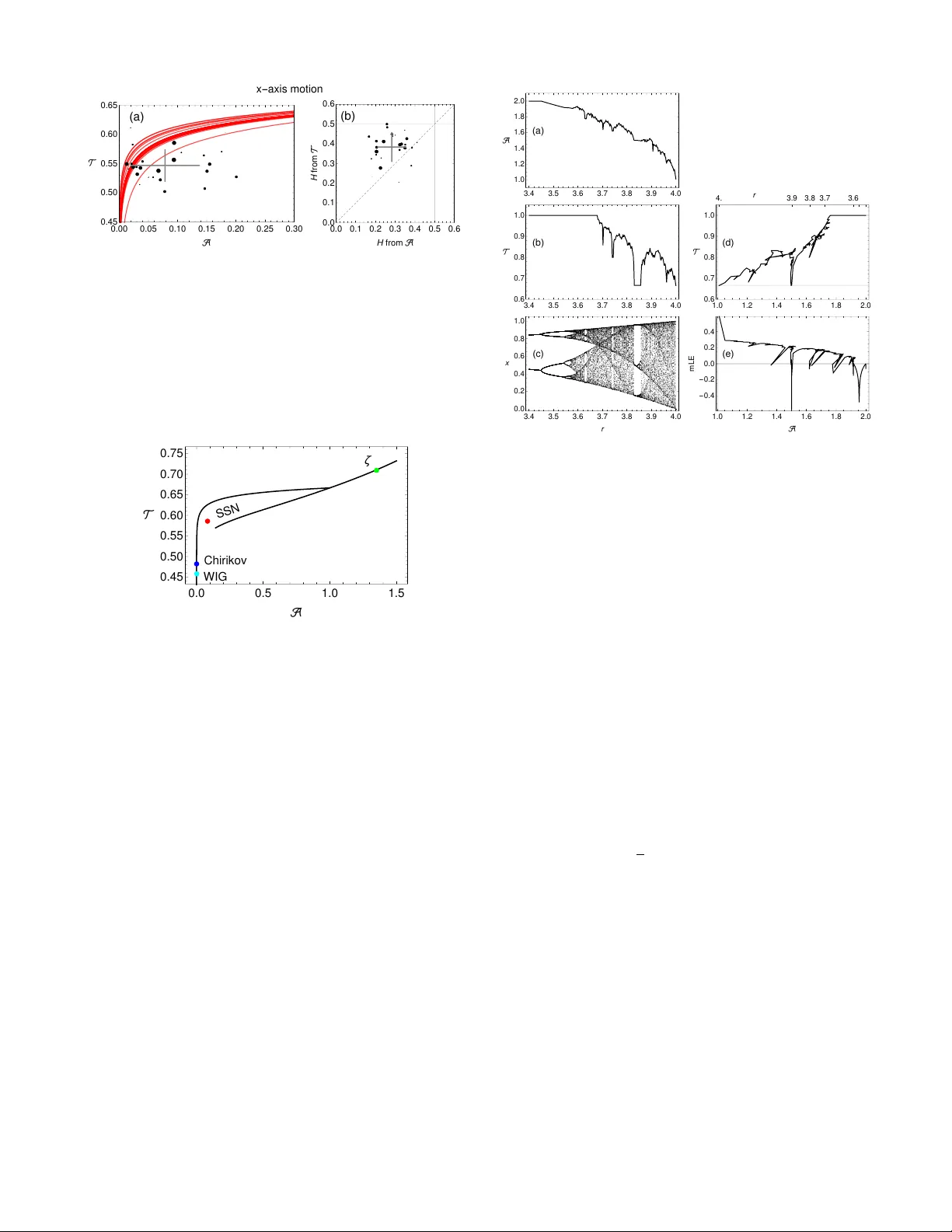
Analytical represen tation of Gaussian pro cesses in the A − T plane ∗ Mariusz T arnop olski † Astr onomic al Observatory, Jagiel lonian University, Orla 171, PL-30-244 Kr ak´ ow, Poland (Dated: Jan uary 1, 2020) Closed-form expressions, parametrized by the Hurst exponent H and the length n of a time series, are derived for paths of fractional Bro wnian motion (fBm) and fractional Gaussian noise (fGn) in the A − T plane, composed of the fraction of turning points T and the Abb e v alue A . The exact formula for A fBm is expressed via Riemann ζ and Hurwitz ζ functions. A very accurate appro ximation, yielding a simple exponential form, is obtained. Finite-size effects, introduced by the deviation of fGn’s v ariance from unit y , and asymptotic cases are discussed. Expressions for T for fBm, fGn, and differen tiated fGn are also presented. The same metho dology , v alid for any Gaussian pro cess, is applied to autoregressiv e moving av erage pro cesses, for which regions of av ailability of the A − T plane are deriv ed and given in analytic form. Lo cations in the A − T plane of some real-w orld examples as w ell as generated data are discussed for illustration. I. INTR ODUCTION The c haracterization and classification of time series [1 – 4] is an imp ortan t task in a v ariet y of fields. Sev eral metho ds hav e b een developed for tasks such as detecting c haos [5], measuring complexity via en tropies [6 – 8], esti- mating the Hurst exp onent [9 – 11], distinguishing chaotic from stochastic pro cesses based on graph theory [12], and more. A connection betw een c haos and long range dep en- dence was also established for low-dimensional c haotic maps [13]. The A − T plane [14], spanned b y the fraction of turn- ing p oin ts T and the Abb e v alue A , w as initially in- tro duced to pro vide a fast and simple estimate of the Hurst exp onen t H , as tigh t relations of b oth A and T with H w ere discov ered for fractional Brownian motion (fBm), fractional Gaussian noise (fGn), and differenti- ated fGn (DfGn). While A ( H ) and T ( H ) strongly ov er- lap for H ∈ (0 , 1) for differen t processes, in the join t space ( A , T ) the fBm and fGn intersect only at the p oin t corresp onding to white noise, i.e. (1 , 2 / 3). A few real- w orld data sets (monthly mean of the sunspot n umber (SSN); sto ck mark et indices; c haotic time series from the Lorenz system and the Chiriko v map) were shown to lie firmly on the fBm branch. Moreov er, the estimates of H based on the empirical relation A ( H ) and computed us- ing a w av elet metho d [15, 16] were consistent with each other. The discriminative p o wer of the A − T plane was demonstrated in a m ultiscale sc heme [17] by employing coarse-grained sequences, i.e. dividing the time series in to nonov erlapping segmen ts of length τ and calculating the mean in each segmen t. This pro duces smo othed se- quences, and the evolution of A and T with v arying tem- p oral scale τ allow ed to separate (i) developed, emerging and fron tier sto c k markets; (ii) healthy and epileptic pa- tien ts based on their EEG recordings—moreov er, for the ∗ Dedicated to my Mother for her 65th birthday . † mariusz.tarnopolski@uj.edu.pl first time it w as possible to distinguish healthy patients with closed and op en ey es; and (iii) patients with and without cardiac diseases based on the heart rate v ari- abilt y . Finally , it is also p ossible to differentiate b et w een c haotic and sto c hastic processes based on the different b eha vior of paths, parametrized by τ , in the A − T plane [18]. The A − T plane is therefore a p o w erful tool with sev eral possible applications. The aim of this pap er is to derive analytical descrip- tions of fBm and fGn, as well as autoregressiv e mo v- ing a verage (ARMA) pro cesses, in the A − T plane. In Sect. II the kno wn facts ab out turning p oints are reca- pitulated. In Sect. I II the exact and appro ximated ex- pressions for A are derived, for the first time, for fBm and fGn. Their A − T plane’s representation is depicted in Sect. IV. ARMA pro cesses are discussed in Sect. V. V arious applications, ranging from pure mathematics, to biology and astroph ysics, to financial markets, are briefly outlined in Sect. VI. Summary and concluding remarks with future prosp ects are gathered in Sect. VI I. I I. FRA CTION OF TURNING POINTS, T A. Theory Consider three v alues x t , x t + d , x t +2 d of a time series { x t } . F or d = 1 the p oin ts are consecutive. Assume there are no ties betw een the neighboring p oin ts, which for con tinuous pro cesses, or empirical data with decent res- olution, should not b e an issue (see also [19, 20]). Three p oin ts can be arranged in six w ays, iden tified b y an order pattern π p (Fig. 1). If the smallest v alue among the three is given an index 1, and the largest an index 3, then e.g. the relation for one of the four p ossible turning p oin ts, x t < x t +2 d < x t + d , is describ ed by a pattern π p = 132. Denote the probabilit y of encoun tering a pattern π p b y p π p . Then the following theorem holds [21]: Theorem 1 F or a Gaussian pr o c ess X t with stationary incr ements, p 123 = p 321 = α/ 2 , and the other p atterns yield pr ob ability (1 − α ) / 4 . 2 123 321 132 231 213 312 FIG. 1. Order patterns for three p oints. The probability p 123 ( d ) for a given delay d is given by p 123 ( d ) = 1 π arcsin r 1 + ρ ( d ) 2 , (1) where the correlation co efficient is ρ ( d ) = E [( X d − X 0 ) ( X 2 d − X d )] E h ( X d − X 0 ) 2 i . (2) The probabilit y T of encountering a turning p oint among three consecutive p oints (i.e., for d = 1, the case consid- ered hereinafter), as p er Theorem 1, is then T = 1 − 2 p 123 (1) . (3) Note that T ∈ [0 , 1]: zero is attained by monotonic se- quences, while unit y is (asymptotically) achiev ed for strictly alternating time series. F or an uncorrelated pro- cess all patterns are equally probable, hence T = 2 / 3. F urther details on order patterns can b e found in [21]. B. T for fBm, fGn, and DfGn With the following prop erties of fBm B ( t ), fGn G ( t ), and DfGn Y ( t ), one can utilize the metho dology from Sect. I I A to calculate T for them as a function of H : E  B 2 ( t )  = t 2 H , (4a) E [ B ( t ) B ( s )] = 1 2  t 2 H + s 2 H − | t − s | 2 H  , (4b) E  G 2 ( t )  =1 , (4c) E [ G ( t ) G ( s )] = 1 2  | t − s − 1 | 2 H + | t − s + 1 | 2 H  − | t − s | 2 H , (4d) E  Y 2 ( t )  =4 − 4 H , (4e) E [ Y ( t ) Y ( s )] = − 3 | t − s | 2 H + 2  | t − s − 1 | 2 H + | t − s + 1 | 2 H  − 1 2  | t − s − 2 | 2 H + | t − s + 2 | 2 H  . (4f ) Eq. (4c) and (4d) can be obtained from Eq. (4a) and (4b) b y substituting G ( t ) = B ( t + 1) − B ( t ); likewise, Eq. (4e) and (4f) follow from Eq. (4c) and (4d) by using Y ( t ) = G ( t + 1) − G ( t ). [22] 0.0 0.2 0.4 0.6 0.8 1.0 0.0 0.2 0.4 0.6 0.8 H  DfGn fGn fBm FIG. 2. F raction of turning p oin ts T for fBm, fGn, and DfGn (red lines). The simulations were p erformed for n = 2 14 (blac k p oin ts). The disp ersion in case of fBm increases for H & 0 . 8 (see [25] for an approximate treatment of the v ariance of T ). F or fBm, one has T fBm = 1 − 2 π arcsin  2 H − 1  , (5) whic h is roughly equal to 2 3 T µ T from [14], where T is the n umber of turning p oints in a time series of length n [2, 23], and µ T = 2 3 ( n − 2) is the exp ected v alue for white noise [24]. In general, E [ T ] = ( n − 2) T . The plot of Eq. (5) is shown in Fig. 2, together with data simulated as in [14] (scaled herein from T /µ T to T ). F or an fGn: T fGn = 1 − 2 π arcsin   1 2 s 3 2 H − 2 2 H +1 − 1 2 2 H − 4   , (6) and for the increments of fGn, i.e. DfGn: T DfGn = 1 − 2 π arcsin   1 2 s (2 2 H + 2) 2 − (2 · 3 H ) 2 3 2 H − 3 · 2 2 H +1 + 15   , (7) b oth of which are also shown in Fig. 2. I II. ABBE V ALUE, A The Abb e v alue of a time series { x i } n i =1 is defined as half the ratio of the mean-square successive difference to the v ariance [14, 26 – 29]: A = 1 n − 1 n − 1 P i =1 ( x i +1 − x i ) 2 2 n n P i =1 ( x i − ¯ x ) 2 . (8) 3 It quantifies the smo othness (raggedness) of a time se- ries by comparing the sum of the squared differences b e- t ween tw o successive measurements with the v ariance of the whole time series. It decreases to zero for time se- ries displaying a high degree of smoothness, while the normalization factor ensures that A tends to unity for a white noise process [30]. It was prop osed as a test for randomness [31 – 33]. It is straightforw ard to sho w that for a 2-p eriodic time series, { a, b, a, b, . . . } , A = 2, while for a 3-p eriodic one, { a, b, c, a, b, c, . . . } , A = 3 / 2. Consider { x i } n i =1 to b e a realization of length n of an fBm, B H n , with Hurst exp onen t H . Thence, its incre- men ts { g i } n − 1 i =1 ≡ { x i +1 − x i } n − 1 i =1 form an fGn, G H n − 1 , with the same H . One can then express A as A fBm ( H , n ) = 1 2 v ar  G H n − 1  v ar ( B H n ) , (9) where the dep endence on H and n is highlighted. Simi- larly , for an fGn A fGn ( H , n ) = 1 2 v ar  Y H n − 1  v ar ( G H n ) , (10) where Y H n − 1 is the corresponding DfGn, i.e. the incre- men ts of fGn, { y i } n − 1 i =1 ≡ { g i +1 − g i } n − 1 i =1 . The goal is to calculate the v ariances of B H n , G H n , and Y H n . A. V ariance of fGn W e start with v ar  G H n  since it o ccurs in b oth Eq. (9) and (10). The same metho dology that was used in [34] to calculate v ar  B H n  is employ ed, i.e. v ar  G H n  = n n − 1 E h  G H n − E  G H n  2 i = 1 n − 1 E      n − 1 X j =0     G j − n − 1 P k =0 G k n     2      . (11) Dev eloping the sum for a few v alues of n , and utilizng the v ariance and cov ariance from Eq. (4c) and (4d), one can observe a pattern emerging, that leads to a formula: v ar  G H n  = n − n 2 H − 1 n − 1 . (12) It yields lim n →∞ v ar  G H n  → 1 , (13) i.e. it asymptotically approac hes Eq. (4c). Ho wev er, for finite n , lim H → 1 v ar  G H n  = 0. The plot of Eq. (12) for n = 2 14 is shown in Fig. 3. F or v alues H & 0 . 8 the departure from the asymptotic v alue becomes significan t. 0.0 0.2 0.4 0.6 0.8 1.0 0.0 0.2 0.4 0.6 0.8 1.0 H var ( G n H ) log 2 n = 14 FIG. 3. Deviation of v ar  G H n  from unity . B. V ariance and Abb e v alue of fBm The v ariance of the discrete, finite length B H n is given in [34] as v ar  B H n  = 1 n ( n − 1) n − 1 X i =1 ( n − i ) i 2 H . (14) F or H → 0, i 2 H → 1; then n − 1 P i =1 ( n − i ) = n ( n − 1) 2 , so v ar  B 0 n  = 1 2 , hence, p er Eq. (9) and giv en Eq. (12), A fBm ( H = 0 , n ) = n/ ( n − 1), i.e. asymptotically ap- proac hes unit y . Using the symbolic computer algebra system Ma th- ema tica one can calculate the sum in Eq. (14) to b e [35] n − 1 X i =1 ( n − i ) i 2 H = ζ ( − 2 H − 1 , n ) − nζ ( − 2 H , n )+ nζ ( − 2 H ) − ζ ( − 2 H − 1) , (15) where ζ ( s ) is the Riemann ζ , and ζ ( s, n ) is the Hurwitz ζ [36]. Hence, taking into account Eq. (12), one can give a closed-form formula: A fBm ( H , n ) = n ( n − 1) 2 v ar  G H n − 1  ζ ( − 2 H − 1 , n ) − nζ ( − 2 H , n ) + nζ ( − 2 H ) − ζ ( − 2 H − 1) , (16) 4 2 4 6 8 10 1 5 10 50 100 500 1000 log 2 n ( a ) H = 0 0.0 0.2 0.4 0.6 0.8 1.0 10 2 10 5 10 8 H ( b ) n = 100 FIG. 4. The ratio from Eq. (18) at (a) H = 0 for v arying n , and (b) its dep endence on H for a set n = 100. whic h, since ζ (0 , n ) = 1 2 − n , ζ ( − 1 , n ) = 1 2  − 1 6 + n − n 2  , ζ (0) = − 1 2 , and ζ ( − 1) = − 1 12 , yields A fBm ( H = 0 , n ) = n/ ( n − 1). In order to provide a simpler, approximate expression for A fBm ( H , n ), first observe that since at H = 0 and for n  1 the ratio of the Hurwitz ζ terms and the Riemann ζ terms is big, i.e. ζ ( − 1 , n ) − nζ (0 , n ) | nζ (0) − ζ ( − 1) | = − 1 + 6 n 2 | 1 − 6 n |  1 , (17) and that for H ∈ (0 , 1) this ratio is monotonically in- creasing (Fig. 4), therefore ζ ( − 2 H − 1 , n ) − nζ ( − 2 H , n ) | nζ ( − 2 H ) − ζ ( − 2 H − 1) |  1 , (18) hence nζ ( − 2 H ) − ζ ( − 2 H − 1) is a negligible contribution, so it do es not need to b e taken into account. Let us express ζ ( s, n ) as a globally conv ergen t Newton series, i.e. utilize the Hasse represen tation [37]: ζ ( s, n ) = 1 s − 1 ∞ X i =0 1 i + 1 i X k =0 ( − 1) k  i k  ( n + k ) 1 − s , (19) v alid for s 6 = 1, n > 0. The first term of the outer sum, i.e. for i = 0 and at s = − 2 H , is 0 X k =0 ( − 1) k  0 k  ( n + k ) 1+2 H = n 1+2 H . (20) The second term, i.e. for i = 1, is 1 2 1 X k =0 ( − 1) k  1 k  ( n + k ) 1+2 H = 1 2  n 1+2 H − ( n + 1) 1+2 H  . (21) And similarly for higher i . Therefore, for i = 0 one ob- tains an approximation ζ ( − 2 H , n ) ≈ n 1+2 H − 2 H − 1 , (22) and for i = 1: ζ ( − 2 H , n ) ≈ 1 − 2 H − 1  3 2 n 1+2 H − 1 2 ( n + 1) 1+2 H  , (23) but since n  1, ( n + 1) ≈ n , so one also obtains ζ ( − 2 H , n ) ≈ n 1+2 H − 2 H − 1 . (24) F or higher i , although giv en that i  n , one has ( n + k ) ≈ n , hence yielding the same approximation. Indeed, i P k =0 ( − 1) k  i k  is the Kroneck er δ , δ i 0 , hence only the i = 0 term surviv es. F or s = − 2 H − 1 one obtains a similar expression: ζ ( − 2 H − 1 , n ) ≈ n 2+2 H − 2 H − 2 . (25) Therefore, with these approximations one can write: ζ ( − 2 H − 1 , n ) − nζ ( − 2 H , n ) ≈ n 2+2 H − 2 H − 2 − nn 1+2 H − 2 H − 1 = n 2+2 H 2( H + 1)(2 H + 1) , (26) so that v ar  B H n  ≈ n 2+2 H 2( H + 1)(2 H + 1) n ( n − 1) , (27) and since ( n − 1) ≈ n , one finally obtains v ar  B H n  ≈ n 2 H 2( H + 1)(2 H + 1) (28) and A fBm ( H , n ) ≈ ( H + 1)(2 H + 1) n − 2 H v ar  G H n − 1  , (29) whic h also yields A fBm ( H = 0 , n ) = n/ ( n − 1), asymptoti- cally approac hing unit y . In case one sets v ar  G H n − 1  = 1, the simplest approximation is then obtained as A fBm ( H , n ) ≈ ( H + 1)(2 H + 1) n − 2 H . (30) These v arious appro ximations of A fBm ( H , n ) are shown in Fig. 5. F or an unreasonably small n = 8 one sees dis- crepancies b etw een the curves for lo w and mo derate H , although they are rather small. The finite-size effects, in tro duced by v ar  G H n  from Eq. (12), are significant at higher v alues of H . F or a mo derate n = 100, the curv es are indistinguishable for most of the range of H , with the region of significan t influence of v ar  G H n  mo ved system- atically to higher H , and for even longer time series (e.g. n = 2 10 ) the consistency of all curves is only strength- ened. Therefore, the approximation from Eq. (30) is a decen t one for time series with any reasonable length. C. V ariance of DfGn and Abb e v alue of fGn T o obtain an expression for v ar  Y H n  the same metho dology from Sect. I II A is undertaken, i.e. Eq. (11) with G changed to Y is employ ed. Again, developing the sum for a few v alues of n , and utilizng the v ariance and co v ariance from Eq. (4e) and Eq. (4f), one can observe the pattern depicted in T able I. Hence one can write 5 exact exact with var ( G )= 1 approx. with var ( G ) approx. with var ( G )= 1 0.0 0.2 0.4 0.6 0.8 1.0 0.01 0.05 0.10 0.50 1 H  ( a ) n = 8 exact exact with var ( G )= 1 approx. with var ( G ) approx. with var ( G )= 1 0.0 0.2 0.4 0.6 0.8 1.0 10 - 6 10 - 5 10 - 4 10 - 3 10 - 2 10 - 1 10 0 H  ( b ) n = 100 exact exact with var ( G )= 1 approx. with var ( G ) approx. with var ( G )= 1 0.0 0.2 0.4 0.6 0.8 1.0 10 - 11 10 - 9 10 - 7 10 - 5 10 - 3 10 - 1 H  ( c ) n = 1024 FIG. 5. A ( H, n ) for (a) an extremely short ( n = 8) fBm time series, for (b) a mo derate ( n = 100), and (c) a long one ( n = 2 10 ). The ”exact” line (red) corresp onds to Eq. (16), ”exact with v ar( G ) = 1” to the same Eq. (16) but with v ar  G H n  = 1, i.e. set to its asymptotic v alue (blue), the ”approx. with v ar( G )” denotes Eq. (29) with the expression for v ar  G H n  included (green), and ”appro x. with v ar( G ) = 1” is the most simplified form from Eq. (30) (cyan). The lines ov erlap so strongly that for visualization purp oses they are depicted with different thickness. v ar  Y H n  = 2(2 n 2 − 1) − n 2 2 2 H + ( n − 1) 2 H − 2 n 2 H + ( n + 1) 2 H n ( n − 1) . (31) The exact expression for the Abb e v alue, taking into ac- coun t Eq. (12), is thence A fGn ( H , n ) = n 2 H + ( n − 2) 2 H + n ( n − 2)  4 − 4 H  − 2( n − 1) 2 H + 2 − 2 2 H 2( n − 2) ( n − n 2 H − 1 ) (32) exact approx. 0.0 0.2 0.4 0.6 0.8 1.0 0.0 0.5 1.0 1.5 2.0 2.5 3.0 H var ( Y n H ) ( a ) log 2 n = 5 exact approx. 0.0 0.2 0.4 0.6 0.8 1.0 0.0 0.5 1.0 1.5 2.0 2.5 3.0 H var ( Y n H ) ( b ) log 2 n = 14 FIG. 6. v ar  Y H n  for (a) a v ery short ( n = 32) time series, and (b) for a long one, n = 2 14 . The ”exact” line (black) is for Eq. (31), and the ”approx.” line (red) denotes Eq. (33). In the limit n → ∞ , i.e. for an y reasonable n  1, Eq. (31) b ecomes v ar  Y H n  ≈ 4 − 4 H , (33) i.e. it asymptotically approac hes Eq. (4e). Plots of Eq. (31) and (33) are sho wn in Fig. 6. F or very short time series there is a certain deviation b etw een the expres- sions, but for higher n the difference is in visible. There- fore, the asymptotic Eq. (33) is adequate in any practical scenario. The Abb e v alue is thence A fGn ( H , n ) ≈ 2 − 2 2 H − 1 v ar ( G H n ) . (34) As discussed in Sect. I II A, the v ariance of G H n can in some instances b e approximated by unit y . Eq. (34) sim- plifies then to just A fGn ( H , n ) ≈ 2 − 2 2 H − 1 , (35) indep enden t on the length n of the time series. The asymptotic Eq. (35) ranges from 0 to 3 / 2 when H decreases from 1 to 0. The expression from Eq. (34) reac hes its maximum of 3 2 n n +1 at H = 0. The asymptotic minim um, as H → 1, is n − 1 n ln 4 ln n = n − 1 n log n 4. F or n = 2 14 , these v alues are 1.49991 and 0.14285, resp ectively , in p erfect agreement with Fig. 3 in [14]. IV. REPRESENT A TION OF FBM AND F GN IN THE A − T PLANE The A−T plane is display ed in Fig. 7. The blac k p oin ts come from sim ulations [14]. In case of fBm [Fig. 7 (a) and 6 T ABLE I. Expressions for v ar  Y H n  for first few n , and the resulting general formula. n n ( n − 1)v ar  Y H n  2 2 · 7 − 2 2 · 2 2 H +1 2 H − 2 · 2 2 H +3 2 H 3 2 · 17 − 3 2 · 2 2 H +2 2 H − 2 · 3 2 H +4 2 H 4 2 · 31 − 4 2 · 2 2 H +3 2 H − 2 · 4 2 H +5 2 H 5 2 · 49 − 5 2 · 2 2 H +4 2 H − 2 · 5 2 H +6 2 H 6 2 · 71 − 6 2 · 2 2 H +5 2 H − 2 · 6 2 H +7 2 H 7 2 · 97 − 7 2 · 2 2 H +6 2 H − 2 · 7 2 H +8 2 H 8 2 · 127 − 8 2 · 2 2 H +7 2 H − 2 · 8 2 H +9 2 H 9 2 · 161 − 9 2 · 2 2 H +8 2 H − 2 · 9 2 H +10 2 H 10 2 · 199 − 10 2 · 2 2 H +9 2 H − 2 · 10 2 H +11 2 H 2(2 n 2 − 1) − n 2 · 2 2 H +( n − 1) 2 H − 2 n 2 H +( n + 1) 2 H (b)], the red line emplo ys the exact formula for A fBm from Eq. (16), while the cy an line depicts the approximation from Eq. (30). Eq. (5) describ es T fBm . In case of fGn [Fig. 7 (c) and (d)], the red line corre- sp onds to the exact Eq. (32) for A fGn , while the cyan line to the asymptotic form from Eq. (35). Eq. (6) describ es T fGn . Panels (b) and (d) of Fig. 7 employ a logarithmic horizon tal axis to fully display the dep endence T ( A ) at small v alues of A (i.e. high v alues of H ). The agreement b et w een n umerical sim ulations and the analytic descrip- tion is very goo d; also the appro ximations for A fGn ( H , n ) w ork well in the A − T plane. In particular, the approx- imation from Eq. (34) for fGn is as go o d as the exact Eq. (32). V. ARMA PROCESSES The methodology from Sect. I I and II I is applicable also to ARMA pro cesses. Generalizing Eq. (8), similarly as was done in Eq. (9) and (10), the Abb e v alue of a pro cess X is A = 1 2 v ar ( dX ) v ar ( X ) , (36) where dX denotes the increments of X . The fraction of turning points is given b y Eq. (1)–(3). It will b e con- v enient to express ρ ( d ) in terms of the auto correlation function ρ d = E [ X ( t ) X ( t + d )]: ρ ( d ) = 2 ρ d − 1 − ρ 2 d 2(1 − ρ d ) , (37) so that Eq. (1) b ecomes p 123 ( d ) = 1 π arcsin  1 2 r 1 − ρ 2 d 1 − ρ d  . (38) This formula can be directly applied also to fGn and DfGn, but not to fBm which is nonstationary . F or ARMA processes, ρ d and v ar ( X ) are easily ob- tainable [2, 3]. The v ariance of the differentiated process, v ar ( dX ), is calculated as v ar ( dX ( t )) = E  dX 2 ( t )  = E h ( X ( t + 1) − X ( t )) 2 i = E  X 2 ( t + 1)  + E  X 2 ( t )  − 2 E [ X ( t + 1) X ( t )] . (39) A. AR(1) Consider a w eakly stationary pro cess X t = a 1 X t − 1 + ε t , − 1 < a 1 < 1, where ε t is a white-noise error term. Then ρ d = a d 1 (40) for all d , thus T = 1 − 2 π arcsin  1 2 √ 1 + a 1  , (41) reac hing its minimum of 1 / 2 when a 1 → 1, and its max- im um of 1 when a 1 → − 1. One then obtains v ar ( X ) = 1 1 − a 2 1 (42) and v ar ( dX ) = 2 1 + a 1 , (43) and thus A = 1 − a 1 , (44) reac hing its minim um of 0 when a 1 → 1, and maximum of 2 when a 1 → − 1. One can then write T explicitly as a function of A : T = 1 − 2 π arcsin  1 2 √ 2 − A  , (45) whic h is display ed in Fig. 8. The Ornstein-Uhlenbeck (OU) pro cess, a contin uous analog of AR(1), yields the same Eq. (45), but restricted to A ∈ [0 , 1] (see Ap- p endix ). B. AR(2) Consider a weakly stationary pro cess X t = a 1 X t − 1 + + a 2 X t − 2 + ε t , − 1 < a 2 < 1 ∧ a 2 < 1 + a 1 ∧ a 2 < 1 − a 1 . Then ρ d is giv en b y a recurren t relation (the Y ule-W alker equations): ρ d =      1 d = 0 a 1 1 − a 2 d = 1 a 1 ρ d − 1 + a 2 ρ d − 2 d ≥ 2 (46) 7 0.0 0.2 0.4 0.6 0.8 1.0 0.56 0.58 0.60 0.62 0.64 0.66   ( a ) - 8 - 6 - 4 - 2 0 0.0 0.1 0.2 0.3 0.4 0.5 0.6 0.7 log 10   ( b ) 0.0 0.5 1.0 1.5 0.55 0.60 0.65 0.70 0.75   ( c ) - 1.2 - 1.0 - 0.8 - 0.6 - 0.4 - 0.2 0.0 0.2 0.55 0.60 0.65 0.70 0.75 log 10   ( d ) FIG. 7. The A − T plane for n = 2 14 : (a)–(b) fBm, (c)–(d) fGn. The red lines utilize the exact expressions for A [i.e. Eq. (16) and (32)], and cyan ones use the approximations [Eq. (30) for fBm and the asymptotic Eq. (35) for fGn]. Eq. (5) and (6) describ e T fBm and T fGn , resp ectiv ely . The horizontal and vertical dashed lines mark T = 2 / 3 and A = 1, resp ectively . P anels (b) and (d) display the same as (a) and (c), but with a logarithmic horizontal axis. The discrepancies in (b) at very low A are due to the deviation of v ar  G H n  from unity when H tends to 1. th us T = 1 − 2 π arcsin  1 2 √ 1 + a 1 − a 2  , (47) reac hing its minimum of 0 when a 1 → 2 , a 2 → − 1, and its maximum of 1 along the line a 2 = a 1 + 1. One then obtains v ar ( X ) = 1 − a 2 ( a 2 + 1)( a 2 − a 1 − 1)( a 2 + a 1 − 1) (48) and v ar ( dX ) = 2 1 + a 1 + a 1 a 2 − a 2 2 , (49) th us A = 1 + a 1 a 2 − 1 , (50) reac hing its minimum of 0 along the line a 2 = 1 − a 1 , and maxim um of 2 along the line a 2 = 1 + a 1 . One cannot write T explicitly as a function of A , as ( A , T ) is a tw o- dimensional region, depicted in Fig. 8. Ho wev er, it is p ossible to give a simple formula for the b oundaries of this region. Note that for a given a 1 , T is minimal when a 2 → − 1. Hence by setting a 2 = − 1, one can then solve Eq. (50) for a 1 , i.e. write a 1 = 2(1 − A ), and insert this in to Eq. (47) to obtain the low er b oundary as T ( A ) low er b oundary = 2 π arcsin r A 2 ! . (51) The upp er boundary , T = 1, is attained when a 2 → 1, and from the left the region is a vertical line A = 0, obtained by sweeping a 2 from − 1 to 1. Notice that AR(1) is a special case of AR(2) with a 2 = 0. One can then observe, by rep eating the ab ov e reason- ing for an arbitrary a 2 , that the region of a v ailability , S AR(2) , is formed as a contin uum of curves parametrized b y a 2 : S AR(2) =  T ( A )   a 2  = ( 1 − 2 π arcsin  1 2 p ( A − 2)( a 2 − 1)       − 1 < a 2 < 1 ) , (52) reducing to Eq. (51) when a 2 → − 1. 8 C. MA(1) Consider X t = b 1 ε t − 1 + ε t , w eakly stationary for all b 1 ∈ R . The auto correlation function is ρ d =      1 d = 0 b 1 1+ b 2 1 d = 1 0 otherwise (53) th us T = 1 − 2 π arcsin 1 2 s 1 + b 2 1 1 − b 1 + b 2 1 ! , (54) reac hing its minimum of 1 / 2 at b 1 = 1, and its maximum of (2 /π ) arcsec √ 6 ≈ 0 . 73 at b 1 = − 1. One then obtains v ar ( X ) = 1 + b 2 1 (55) and v ar ( dX ) = 2 (1 + b 1 ( b 1 − 1)) , (56) th us A = 1 − b 1 + b 2 1 1 + b 2 1 , (57) reac hing its minimum of 1 / 2 at b 1 = 1, and maxim um of 3 / 2 at b 1 = − 1. One can then write T explicitly as a function of A : T = 1 − 2 π arcsin  1 2 √ A  , (58) whic h is display ed in Fig. 8. D. MA(2) Consider X t = b 1 ε t − 1 + b 2 ε t − 2 + ε t , weakly stationary for all b 1 , b 2 ∈ R , for which ρ d =            1 d = 0 b 1 (1+ b 2 ) 1+ b 2 1 + b 2 2 d = 1 b 2 1+ b 2 1 + b 2 2 d = 2 0 otherwise (59) th us T = 1 − 2 π arcsin 1 2 s 1 + b 2 1 + b 2 ( b 2 − 1) 1 + b 2 1 + b 2 2 − b 1 ( b 2 + 1) ! , (60) reac hing its minimum of 2 / 5 at b 1 = 1 2  1 + √ 5  , b 2 = 1, and its maximum of 4 / 5 at b 1 = 1 2  1 − √ 5  , b 2 = 1. One then obtains v ar ( X ) = 1 + b 2 1 + b 2 2 (61) and v ar ( dX ) = 2  1 + b 2 1 + b 2 2 − b 1 ( b 2 + 1)  , (62) th us A = 1 − b 1 ( b 2 + 1) 1 + b 2 1 + b 2 2 , (63) reac hing its minim um of 1 − 1 / √ 2 at b 1 = √ 2 , b 2 = 1, and maxim um of 1 + 1 / √ 2 at b 1 = − √ 2 , b 2 = 1. One cannot write T explicitly as a function of A , as ( A , T ) is a tw o-dimensional region, depicted in Fig. 8. E. ARMA(1,1) Consider X t = a 1 X t − 1 + b 1 ε t − 1 + ε t , weakly stationary for − 1 < a 1 < 1 and all b 1 ∈ R , for which ρ d = ( 1 d = 0 a d − 1 1 ( a 1 + b 1 )( a 1 b 1 +1) 1+2 a 1 b 1 + b 2 1 otherwise (64) th us T = 1 − 2 π arcsin 1 2 s (1 + a 1 )(1 + a 1 b 1 + b 2 1 ) 1 + b 1 ( a 1 + b 1 − 1) ! , (65) reac hing its minim um of 1 / 3 when a 1 → 1 , b 1 = 1, and its maximum of 1 when a 1 → − 1, along the line b 1 ∈ R . One then obtains v ar ( X ) = 1 + 2 a 1 b 1 + b 2 1 1 − a 2 1 (66) and v ar ( dX ) = 2 1 + b 1 ( a 1 + b 1 − 1) a 1 + 1 , (67) th us A = 1 − a 1 + b 1 ( a 2 1 − 1) 1 + 2 a 1 b 1 + b 2 1 , (68) reac hing its minimum of 0 when a 1 → 1, along the line b 1 ∈ R , and maximum of 2 when a 1 → − 1, along the line b 1 ∈ R . One cannot write T explicitly as a function of A , as ( A , T ) is a tw o-dimensional region, depicted in Fig. 8. Note that Eq. (65) and (68) are inv ariant on changing b 1 to 1 /b 1 , so that in the context of geometrical depiction of the region of a v ailabilit y only the range − 1 ≤ b 1 ≤ 1 needs to b e considered. Roughly speaking, cases with | b 1 |  1 are equiv alen t to | b 1 |  1. How ev er, b 1 = ± 1 are sp ecial instances: • when b 1 = − 1, Eq. (68) yields a 1 = 3 − 2 A , whic h fulfills the stationarity condition, a 1 ∈ ( − 1 , 1), only for A ∈ (1 , 2). In this range: T ( b 1 = − 1) = 1 − 2 π arcsin 1 2 r 5 − 2 A − 2 A ! ; (69) 9 • likewise, when b 1 = 1, one obtains a 1 = 1 − 2 A , whic h le ads to A ∈ (0 , 1), giving: T ( b 1 = 1) = 1 − 2 π arcsin  1 2 √ 3 − 2 A  . (70) In particular, b 1 = 0 reduces an ARMA(1,1) pro cess to an AR(1) one, repro ducing respective formulae from Sect. V A. Similarly as was done in Sect. V B for AR(2) pro cesses, the region of av ailabity for ARMA(1,1) can b e describ ed as a contin uum of curves, S ARMA(1 , 1) =  T ( A )   b 1  , parametrized by b 1 : one needs to solve Eq. (68) for a 1 and insert the solution into Eq. (65). The resulting formula, easy to derive but of a quite complicated and noninfor- mativ e form, is not display ed herein. VI. APPLICA TIONS A. Bacterial cytoplasm The t wo-dimensional motion [ x ( t ) , y ( t )] of individual mRNA molecules inside live Escherichia c oli bacteria w ere track ed in [38]. It was found that they follow anoma- lous diffusion, with H < 0 . 5, confirmed b y other metho ds as well [39]. Herein, the time series x and y are treated separately . Results for the 27 tracks are displa y ed in Fig. 9 for the x -axis. Similar outcomes w ere obtained for the y -axis. The lo cations in the A − T plane are in agree- men t with an fBm description, and the v alues extracted using Eq. (5) and (30), yielding 0 . 2 . H . 0 . 5, are con- sisten t with each other, and confirm that the observ ed pro cess is indeed sub diffusiv e. B. Zeros of the Riemann ζ The first 10 6 + 1 nontrivial zeros, 1 2 + i γ n , of the Rie- mann ζ function [40] w ere retrieved [41]. Normalized spacings b et ween consecutive zeros were computed as [42] δ n = γ n +1 − γ n 2 π ln  γ n 2 π  . (71) The lo cation of this sequence in the A − T plane is (1 . 350 , 0 . 709). This is remark ably close to the fGn line (Fig. 10), and Eq. (6) and (35) give H = 0 . 19. In compar- ison, the discrete wa v elet transform (DWT) metho d [14] returns H = 0 . 06, hence also strongly implying H < 0 . 5. Ho wev er, as the distribution of δ n is not normal, but rather follo ws the distribution of the Gaussian unitary ensem ble (GUE) according to the GUE hypothesis [43], so this sequence is not a Gaussian pro cess, strictly sp eak- ing. Note, ho w ever, that a lo cation in the A − T plane can b e computed for any type of data; in this case, due to A > 1 and T > 2 / 3, one gets a clear information that the series is—in a sense—(muc h) more noisy than regular white noise. 0.0 0.5 1.0 1.5 2.0 0.0 0.2 0.4 0.6 0.8 1.0   ( a ) AR ( 2 ) ARMA ( 1,1 ) MA ( 2 ) MA ( 1 ) AR ( 1 )  0.0 0.5 1.0 1.5 2.0 0.0 0.2 0.4 0.6 0.8 1.0 ( b ) 0.0 0.5 1.0 1.5 2.0 0.0 0.2 0.4 0.6 0.8 1.0 ( c ) 0.0 0.5 1.0 1.5 2.0 0.0 0.2 0.4 0.6 0.8 1.0 ( d ) 0.0 0.5 1.0 1.5 2.0 0.0 0.2 0.4 0.6 0.8 1.0 ( e ) 0.0 0.5 1.0 1.5 2.0 0.0 0.2 0.4 0.6 0.8 1.0 ( f )  FIG. 8. (a) Regions of the A − T plane av ailable for ARMA pro cesses: AR(1) (red line), MA(1) (blue line), MA(2) (dark er gra y region), AR(2) (light blue in the background), and ARMA(1,1) (ligh ter gra y region). The blac k dotted line in the range A ∈ (0 , 1) is Eq. (70) for ARMA(1,1) with b 1 = 1, and the black dashed line in A ∈ (1 , 2) is Eq. (69) for ARMA(1,1) with b 1 = − 1. These tw o lines mark the low er b oundary of the region of a v ailabilit y for the ARMA(1,1) process. The y ellow dot at (1 , 2 / 3) denotes white noise. In the other pan- els, these regions are shown together with locations of 10 3 sim ulated processes: (b) AR(1), (c) MA(1), (d) AR(2), (e) MA(2), and (f ) ARMA(1,1). In the simulations, the AR co- efficien ts were dra wn uniformly from the resp ectiv e regions fulfilling the stationarity conditions, and the MA coefficients w ere drawn uniformly from ( − 1 , 1). Note the v arying density of p oints in the regions of av ailability . C. Sunsp ot n umbers The curen tly a v ailable from the W orld Data Cen ter Sunsp ot Index and Long-term Solar Observ ations [44] sample of 3250 monthly SNN are describ ed by H = 0 . 3, as computed with the DWT approac h [45]. The loca- 10 ● ● ● ● ● ● ● ● ● ● ● ● ● ● ● ● ● ● ● ● ● ● ● ● ● ● ● ● ● ● ● ● ● ● ● ● ● ● ● ● ● ● ● ● ● ● ● ● ● ● ● ● ● ● 0.00 0.05 0.10 0.15 0.20 0.25 0.30 0.45 0.50 0.55 0.60 0.65   ( a ) ● ● ● ● ● ● ● ● ● ● ● ● ● ● ● ● ● ● ● ● ● ● ● ● ● ● ● ● ● ● ● ● ● ● ● ● ● ● ● ● ● ● ● ● ● ● ● ● ● ● ● ● ● ● 0.0 0.1 0.2 0.3 0.4 0.5 0.6 0.0 0.1 0.2 0.3 0.4 0.5 0.6 H from  H from  ( b ) x - axis motion FIG. 9. (a) Lo cations in the A − T plane of the 27 tracks of x -axis motion of mRNA molecules inside E. c oli . The red lines are the fBm lines, corresp onding to the length of time series 140 ≤ n ≤ 1628. Lo wer curves corresp ond to low er n . (b) Estimated H v alues, obtained from the formulae for A and T , i.e. Eq. (30) and (5), resp ectiv ely . In b oth panels, the size of the p oin t is prop ortional to n . The gray crosses sym b olize the (unw eigh ted) means and standard deviations of the display ed lo cations. 0.0 0.5 1.0 1.5 0.45 0.50 0.55 0.60 0.65 0.70 0.75   ζ SSN Chirikov WIG FIG. 10. Locations of some real-world and generated time series. The black lines corresp ond to fBm and fGn with n = 2 14 . See text for details. tion in the A − T plane is (0 . 082 , 0 . 586), Fig. 10, and Eq. (5) and (30) give H ≈ 0 . 18 − 0 . 27. This is in agree- men t with some works [46] that also compute H < 0 . 5. Note that the SSN sequence is slightly off the fBm line, hence it not necessarily need to b e adequately mo deled b y an fBm pro cess. The SSN is a straightforw ard wa y of monitoring the Sun’s activity , and since the sunsp ots are tigh tly connected with the magnetic fields gov erning so- lar flares and coronal mass ejections, its prop er mo deling is crucial in forecasting the space weather conditions. D. Chaos The Chiriko v standard map for a chaotic state (in an un b ounded setting) was examined in [14]. Its lo cation in the A − T plane is (0 . 0002 , 0 . 482), and lies directly on the fBm line, Fig. 10, and Eq. (5) and (30) give H ≈ 0 . 5, which is in p erfect agreement with the estimate with D WT method, yielding H = 0 . 48. This means that, in the con text of long-term memory , it is uncorrelated, and acts like Brownian motion. 3.4 3.5 3.6 3.7 3.8 3.9 4.0 1.0 1.2 1.4 1.6 1.8 2.0  ( a ) 3.4 3.5 3.6 3.7 3.8 3.9 4.0 0.6 0.7 0.8 0.9 1.0  ( b ) 1.0 1.2 1.4 1.6 1.8 2.0 0.6 0.7 0.8 0.9 1.0 3.6 3.7 3.8 3.9 4.  r ( d ) 3.4 3.5 3.6 3.7 3.8 3.9 4.0 0.0 0.2 0.4 0.6 0.8 1.0 r x ( c ) 1.0 1.2 1.4 1.6 1.8 2.0 - 0.4 - 0.2 0.0 0.2 0.4  mLE ( e ) FIG. 11. Relations b et ween A , T , r , and mLE for the logistic map. T o further illustrate c haotic behavior in the A − T plane, the logistic map x i +1 = r x i (1 − x i ) is consid- ered. F or r ∈ [3 . 4 , 4 . 0], with a step ∆ r = 0 . 002, time series of length n = 10 4 w ere generated and their ( A , T ) lo cations, as well as the maximal Ly apuno v exp onen ts (mLEs), w ere computed. The dep endencies of A and T on r , the bifurcation diagram, the A − T plane, and the relation b et ween A and mLE, are sho wn in Fig. 11. When chaos is most dev elop ed ( r = 4), the tra jectories approac h the p oint ( A , T ) = (1 , 2 / 3), identical for white noise [Fig. 11(d)]. Hints that fully developed c haos b e- ha ves this wa y were noted in case of the Lorenz system [14, 17]. With increasing r , a gradual decrease in T o c- curs, with w ells in perio dic windows [Fig. 11(b)]. Note that T = 1 up to r . 3 . 7, b ecause apparently the orbits, ev en when c haotic, are strictly alternating. A is more sensitiv e to changes in dynamics, as A = 2 for p eriod-2 orbits (see the b eginning of Sect. I I I) b efore the bifur- cation at r = 1 + √ 6 ≈ 3 . 45, and then systematically decreases in the p erio d-4 windo w b efore the next bifurca- tion at r ≈ 3 . 54 [Fig. 11(a)]. There are also shallow w ells at perio dic windo ws within the c haotic zone. The path in the A − T plane is jagged, and v arious c hanges in dynam- ics are manifested, corresp onding to c hanges in mLEs [Fig. 11(e)] and in the bifurcation diagram [Fig. 11(c)]. A tight, positive correlation b et ween mLE and H for the Chiriko v map was discov ered [13] (see also [47]). Differences b et w een (quasi)p eriodic and chaotic systems w ere observed in the coarse-grained sequences in the A − T plane in case of a sin usoidally driven thermo- stat [18]. These connections b et ween c haos, H , and the A − T plane are nontrivial, and require further research. Describing a universal (if existen t) b ehavior of c haotic 11 3 4 5 6 0.450 0.455 0.460 0.465 10 3   FIG. 12. Time ev olution of the WIG. The green dot marks the start p oint, and the red dot denotes the end p oint. Note the scale of the horizontal axis. See text for details. systems in the A − T plane in an interesting persp ec- tiv e. The p ossibilit y of differen tiating b et ween chaotic and sto chastic time series is a hop efully attainable appli- cation. E. Mark ets The efficien t market h ypothesis [48] is a key concept in finance. If a mark et exhibits H 6 = 0 . 5, then it might allo w arbitrage. A classification of dev elop ed, emerging and fron tier sto ck mark ets in the A − T plane was p erformed in [17], and show ed that these three categories of markets o ccup y distinct regions of the ( A , T ) space. Hence, the A − T plane is a useful tool for classifying data with differen t underlying dynamics. The time evolution of H of many sto ck markets shows it is oscillating around H = 0 . 5 [10]. Similarly , one can in vestigate how A and T evolv e, and hence trace their v alues in the A − T plane at differen t times. As an exam- ple consider the W arsaw Stock Exc hange Index (W arsza- wski Indeks Gie ldowy , WIG) [49]. Its location in the A − T plane, right on the fBm line, is depicted in Fig. 10, and the estimates of H , obtained by solving Eq. (5) and (30) with n = 2166, yield H ≈ 0 . 49 − 0 . 59. The DWT metho d returns H = 0 . 48. The time evolution is depicted in Fig. 12. It is obtained by partitioning the whole time series into o verlapping segments of size n/ 2, adv ancing eac h segmen t by one p oint. Throughout its history , the WIG remains confined in a small region of the A − T plane. F. Activ e galactic n uclei A core fo cus in astronom y is the in v estigation of ap- paren t v ariability of v arious celestial ob jects such as as- teroids, stars, or galaxies. Within the latter, of partic- ular in terest are active galactic nuclei (AGNs), further divided in to sev eral types [50]. Among them, blazars are p eculiar AGNs p oin ting their relativistic jets tow ard the Earth. Blazars are commonly divided further into t wo subgroups, i.e. flat sp ectrum radio quasars (FSRQs) and BL Lacertae (BL Lac) ob jects, based on character- istics visible in their optical sp ectra. In a recent study [51] it was found that fain t FSR Q and BL Lac candi- dates lo cated b ehind the Magellanic Clouds are clearly separated in the A − T plane, with means of A ≈ 0 . 3 and A ≈ 0 . 7, resp ectively . This differen tiation, based solely on the temp oral data in the form of light curv es, is another pro of that employing the A − T plane as a classification to ol is a promising approach. G. Other The w orked-out examples from Sect. VI A–VI F do not exhaust the p ossible applications of the A − T plane in regard to constraining the v alue of H , or classifying time series. Some other in teresting instances include, but are not restricted to: ferro- and paramagnetic states of the Heisen b erg mo del that exhibit H ∼ 1 and H ∼ 0 . 5, re- sp ectiv ely [52], and should b e easily distinguishable in the A − T plane; a photonic in tegrated circuit yields 0 . 2 . H . 0 . 8 for v aried electric field of the feed- bac k, coupled with chaotic b ehavior [53]; cataclysmic v ariable stars observ ed in X-ra ys exhibit long-term mem- ory , H > 0 . 5, suggesting the accretion is driven by mag- netic fields [54]; fo otball matc hes can follow the rules of fBm with H ∼ 0 . 7 [55]; p ersistence of amo eb oid motion [56] as w ell as Nitzschia sp. diatoms [57]; Solar wind pro- ton density fluctuations are c haracterized b y H ∼ 0 . 8, placing constrain ts on the mo dels of kinetic turbulence [58]; v alues H > 0 . 5 w ere computed for epileptic pa- tien ts’ brain activity , quantified via magneto encephalo- graphic recordings, and app ear to b e a promising addi- tional diagnostic to ol for identifying epileptogenic zones in presurgical ev aluation [59]. Recall that epilepsy has b een already inv estigated in the A − T plane as well [17]. VI I. SUMMAR Y AND OPEN QUESTIONS Exact analytical descriptions for the lo cations of fBm and fGn in the A − T plane were deriv ed. W orking ap- pro ximations were also obtained in the following forms: ( A fBm ( H , n ) = ( H + 1)(2 H + 1) n − 2 H T fBm ( H ) = 1 − 2 π arcsin  2 H − 1  (72) and ( A fGn ( H ) = 2 − 2 2 H − 1 T fGn ( H ) = 1 − 2 π arcsin  1 2 q 3 2 H − 2 2 H +1 − 1 2 2 H − 4  (73) and were demonstrated to be adequate for time series with any reasonable length n . This allo ws to classify time series of any length, resp ective to fBm and fGn, without relying on time-consuming numerical simulations. These analyses add to the theoretical results regarding fBm and fGn [60, 61]. The same metho dology was applied 12 to ARMA( p, q ) processes. Analytic descriptions of the a v ailable regions of the A − T plane were derived and illustrated for p + q ≤ 2. F urther researc h on A is required, as it has b een rarely utilized, with some recent, nonextensive examples in as- tronom y [29, 51, 62 – 64] (but see also [65]). The interre- lations b etw een ordinal patterns, persistence, and chaos [8, 66] are linked even tigh ter with the bidimensional sc heme of the A − T plane. The presen ted methodol- ogy is v alid for any Gaussian process, but it should be emphasized that the locations ( A , T ) can b e computed for arbitrary time series, serving e.g. as classification or clustering metho ds for empirical data. Naturally , a question ab out A − T representations of other sto chastic pro cesses arises. Examples include the follo wing: • Representation of colored noise, i.e. p ow er sp ectral densities (PSDs) of the form 1 /f β . fBm can b e as- so ciated with β ∈ (1 , 3), and fGn is characterized b y β ∈ ( − 1 , 1). How ev er, p ow er laws are ubiquitu- ous in nature, hence their lo cations in the A − T plane, for any β , is an interesting and c hallenging problem. • In some fields, e.g. in astronom y , the observ ed signals often yield PSDs of the form 1 /f β + C , where C is the so called Poisson noise lev el, coming from the statistical noise due to uncertainties in the measuremen ts; ab o ve a certain frequency , the PSD transitions from a p ow er la w to white noise. A rep- resen tation of such pro cesses in the A − T plane is crucial in classifying light curves of several sources, e.g. A GN. • Other contin uous-time mo dels, e.g. con tinuous ARMA [67], ha v e been dev elop ed. The simplest in this family is the OU pro cess, which is a contin- uous analog of the AR(1) process, with the same A − T representation. In tro ducing long-term mem- ory leads to con tinuous autoregressive fractionally in tegrated mo ving av erage mo dels [68]. A CKNOWLEDGMENTS The author thanks Ido Golding for providing the data of the mRNA motion inside the bacteria. Supp ort b y the P olish National Science Cen ter through OPUS Gran t No. 2017/25/B/ST9/01208 is ackno wledged. App endix: Ornstein-Uhlen b ec k pro cess The OU pro cess with mean µ is given by the sto chastic differen tial e quation d x t = θ ( µ − x t ) d t + σ d ε t , (A.1) where θ > 0 and σ > 0. The correlation function for lag d is ρ d = exp ( − θ d ) , (A.2) whic h via Eq. (38) and (3) leads to T OU ( θ ) = 1 − 2 π arcsin  1 2 p 1 + exp ( − θ )  , (A.3) reac hing its minimum of 1 / 2 for θ = 0, and its maximum of 2 / 3 when θ → ∞ . The cov ariance function E [ x t x s ] = σ 2 2 θ exp ( − θ | t − s | ) (A.4) giv es via Eq. (36) and (39) and on simplification A OU ( θ ) = 1 + sinh θ − cosh θ , (A.5) reac hing its minim um of 0 for θ = 0, and its maxim um of 1 when θ → ∞ . Eq. (A.5) can be solv ed for θ and inserted into Eq. (A.3), which yields Eq. (45), v alid for A ∈ [0 , 1]. [1] J. Beran, Statistics for Long Memory Pro c esses (Chap- man and Hall, New Y ork, 1994). [2] P . J. Bro ckw ell and R. A. Davis, Time Series: The ory and Metho ds, 2nd e d. (Springer-V erlag New Y ork, 1996). [3] P . J. Brockw ell and R. A. Davis, Intr o duction to Time Se- ries and F or e c asting, 2nd e d. (Springer-V erlag New Y ork, 2002). [4] J. Beran, Y. F eng, S. Ghosh, and R. Kulik, L ong Memory Pr o c esses: Pr ob abilistic Pr op erties and Statistic al Meth- o ds (Springer-V erlag, Berlin Heidelb erg, 2013). [5] R. Hegger, H. Kantz, and T. Schreiber, Chaos 9 , 413 (1999). [6] C. Bandt and B. Pompe, Ph ysical Review Letters 88 , 174102 (2002). [7] J. E. Maggs and G. J. Morales, Plasma Ph ysics and Con- trolled F usion 55 , 085015 (2013). [8] H. V. Rib eiro, M. Jauregui, L. Zunino, and E. K. Lenzi, Ph ysical Review E 95 , 062106 (2017). [9] I. Simonsen, A. Hansen, and O. M. Nes, Physical Review E 58 , 2779 (1998), cond-mat/9707153. [10] A. Carbone, G. Castelli, and H. E. Stanley, Ph ysica A: Statistical Mechanics and its Applications 344 , 267 (2004). [11] S. Arianos and A. Carb one, Physica A: Statistical Me- c hanics and its Applications 382 , 9 (2007). [12] L. Lacasa and R. T oral, Physical Review E 82 , 036120 (2010). [13] M. T arnop olski, Physica A: Statistical Mechanics and its Applications 490 , 834 (2018). [14] M. T arnop olski, Physica A: Statistical Mechanics and its 13 Applications 461 , 662 (2016). [15] C.-K. Peng, S. V. Buldyrev, S. Havlin, M. Simons, H. E. Stanley, and A. L. Goldb erger, Physical Review E 49 , 1685 (1994). [16] C.-K. Peng, S. Havlin, H. E. Stanley , and A. L. Gold- b erger, Chaos 5 , 82 (1995). [17] L. Zunino, F. Oliv ares, A. F. Bariviera, and O. A. Rosso, Ph ysics Letters A 381 , 1021 (2017). [18] Y. Zhao and G. J. Morales, Physical Review E 98 , 022213 (2018). [19] L. Zunino, F. Oliv ares, F. Sc holkmann, and O. A. Rosso, Ph ysics Letters A 381 , 1883 (2017). [20] F. T ra versaro, F. O. Redelico, M. R. Risk, A. C. F rery, and O. A. Rosso, Chaos 28 , 075502 (2018). [21] C. Bandt and F. Shiha, Journal of Time Series Analysis 28 , 646 (2007). [22] In the deriv ation of T fGn and T DfGn one can actually em- plo y only the relations for fBm; the calculations would then b ecome quite burdensome, though. [23] M. Kendall and A. Stuart, The advanc e d the ory of statis- tics (London: Griffin, 3rd ed., 1973). [24] The first and last p oin ts cannot form a turning p oint, hence the subtraction of 2 in µ T . [25] M. Sinn and K. Keller, arXiv e-prints , (2008), arXiv:0801.1598 [math.PR]. [26] J. von Neumann, The Annals of Mathematical Statistics 12 , 153 (1941). [27] J. von Neumann, The Annals of Mathematical Statistics 12 , 367 (1941). [28] M. G. Kendall, Biometrik a 58 , 369 (1971). [29] N. Mo wlavi, Astronomy & Astroph ysics 568 , A78 (2014). [30] J. D. Williams, The Annals of Mathematical Statistics 12 , 239 (1941). [31] C. Bingham and L. S. Nelson, T ec hnometrics 23 , 285 (1981). [32] R. Bartels, Journal of the American Statistical Asso cia- tion 77 , 40 (1982). [33] A. Mateus and F. Caeiro, “Exact and approximate prob- abilities for the null distribution of bartels randomness test,” in R e c ent Studies on Risk Analysis and Statisti- c al Mo deling , edited b y T. A. Oliv eira, C. P . Kitsos, A. Oliv eira, and L. Grilo (Springer International Pub- lishing, Cham, 2018) pp. 227–240. [34] D. Deligni` eres, Mathematical Problems in Engineering 2015 , 485623 (2015). [35] See also www.wolframalpha.com . [36] T. M. Ap ostol, Intr o duction to Analytic Numb er Theory (Springer Science+Business Media New Y ork, 1976). [37] H. Hasse, Mathematische Zeitschrift 32 , 458 (1930). [38] I. Golding and E. C. Cox, Ph ysical Review Letters 96 , 098102 (2006). [39] M. Magdziarz, A. W eron, K. Burnecki, and J. Klafter, Ph ysical Review Letters 103 , 180602 (2009). [40] D. J. Platt, Mathematics of Computation 84 , 1521 (2015). [41] https://www.lmfdb.org/zeros/zeta/ . [42] A. M. Odlyzko, Mathematics of Computation 48 , 273 (1987). [43] H. L. Montgomery , in Analytic numb er the ory , Proc. Symp os. Pure Math., XXIV, Providence, R.I.: American Mathematical So ciety , V ol. 24, edited by H. G. Diamond (1973) pp. 181–193. [44] SILSO W orld Data Center, Roy al Observ atory of Bel- gium, Brussels, http://www.sidc.be/silso . [45] Similar v alue can b e obtained with data in [14] when the t wo outliers on the left of Fig. 6b therein are discarded. [46] M. S. Mo v ahed, G. R. Jafari, F. Ghasemi, S. Rah v ar, and M. R. R. T abar, Journal of Statistical Mechanics: Theory and Exp erimen t 2006 , P02003 (2006). [47] W.-H. Steeb and E. C. Andrieu, Zeitschrift Natur- forsc hung T eil A 60 , 252 (2005). [48] R. N. Man tegna and H. E. Stanley , An Intr o duction to Ec onophysics: Corr elations and Complexity in Financ e (Cam bridge Universit y Press, New Y ork, 2000). [49] https://www.investing.com/indices/ wig- historical- data , accessed on Nov ember 10, 2019. [50] C. M. Urry and P . Pado v ani, Publications of the Astro- nomical So ciety of the Pacific 107 , 803 (1995). [51] N. ˙ Zywuc k a, M. T arnop olski, M. B¨ ottcher, L. Staw arz, and V. Marchenk o, arXiv e-prints , (2019), arXiv:1912.03530 [astro-ph.GA]. [52] Z. Zhang, O. G. Mouritsen, and M. J. Zuck ermann, Ph ysical Review E 48 , R2327 (1993). [53] K. E. Chlouverakis, A. Argyris, A. Bogris, and D. Syvridis, Physical Review E 78 , 066215 (2008). [54] G. Anzolin, F. T amburini, D. de Martino, and A. Bian- c hini, Astronomy and Astroph ysics 519 , A69 (2010), arXiv:1005.5319 [astro-ph.SR]. [55] A. Kijima, K. Y ok o yama, H. Shima, and Y. Y a- mamoto, Europ ean Ph ysical Journal B 87 , 41 (2014), arXiv:1402.0912 [physics.pop-ph]. [56] N. Mak ara v a, S. Menz, M. Thev es, W. Huisinga, C. Beta, and M. Holschneider, Ph ysical Review E 90 , 042703 (2014). [57] J. S. Murgu ´ ıa, H. C. Rosu, A. Jimenez, B. Guti ´ errez- Medina, and J. V. Garc ´ ıa-Meza, Physica A: Statis- tical Mechanics and its Applications 417 , 176 (2015), arXiv:1410.3135 [q-bio.QM]. [58] F. Carb one, L. Sorriso-V alv o, T. Alb erti, F. Lepreti, C. H. K. Chen, Z. N ˇ emeˇ cek, and J. ˇ Safr´ anko v´ a, As- troph ysical Journal 859 , 27 (2018), [ph ysics.space-ph]. [59] C. Witton, S. V. Sergeyev, E. G. T uritsyna, P . L. F ur- long, S. Seri, M. Bro ok es, and S. K. T uritsyn, Journal of Neural Engineering 16 , 056019 (2019). [60] L. Zunino, D. G. P´ erez, M. T. Mart ´ ın, M. Garav aglia, A. Plastino, and O. A. Rosso, Physics Letters A 372 , 4768 (2008). [61] T. Sadhu, M. Delorme, and K. J. Wiese, Phys. Rev. Lett. 120 , 040603 (2018). [62] M.-S. Shin, M. Sek ora, and Y.-I. Byun, Monthly Notices of the Roy al Astronomical So ciety 400 , 1897 (2009). [63] K. V. Sokolo vsky, P . Gavras, A. Karamp elas, S. V. An tipin, I. Bellas-V elidis, P . Benni, A. Z. Bonanos, A. Y. Burdano v, S. Derlopa, D. Hatzidimitriou, A. D. Khokhry ako v a, D. M. Kolesniko v a, S. A. Korotkiy , E. G. Lapukhin, M. I. Moretti, A. A. Popov, E. Pouliasis, N. N. Samus, Z. Sp etsieri, S. A. V eselko v, K. V. V olko v, M. Y ang, and A. M. Zubarev a, Monthly Notices of the Ro yal Astronomical So ciety 464 , 274 (2017). [64] M. F. P´ erez-Ortiz, A. Garc ´ ıa-V arela, A. J. Quiroz, B. E. Sab ogal, and J. Hern´ andez, Astronomy & Astrophysics 605 , A123 (2017). [65] J. Lafler and T. D. Kinman, Astrophysical Journal Sup- plemen t 11 , 216 (1965). [66] M. Zanin, L. Zunino, O. A. Rosso, and D. P ap o, Entrop y 14 14 , 1553 (2012). [67] P . J. Bro ckw ell, Annals of the Institute of Statistical Mathematics 66 , 647 (2014). [68] H. Tsai, Bernoulli 15 , 178 (2009).