Evolutionary Clustering via Message Passing

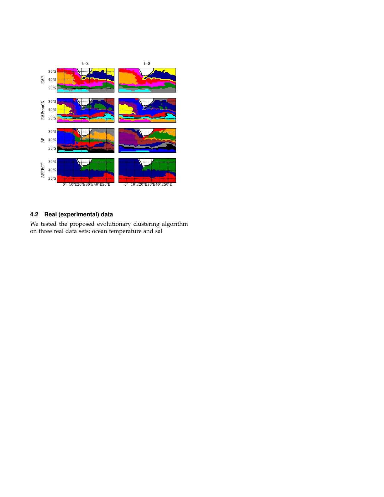
EV OLUTIONAR Y CLUSTERING VIA MESSA GE P ASSING 1 Ev olutionar y Cluster ing via Message P assing Natalia M. Arzeno and Haris Vikalo , Senior Member , IEEE Abstract —We are often interested in clustering objects that e volve o ver time and identifying solutions to the clustering problem f or ev er y time step . Evolutionary clustering provides insight into cluster ev olution and temporal changes in cluster memberships while enabling perf or mance superior to that achiev ed by independently clustering data collected at different time points. In this paper w e introduce ev olutionar y afﬁnity propagation (EAP), an e volutionary clustering algor ithm that groups data points b y e xchanging messages on a factor g raph. EAP promotes temporal smoothness of the solution to clustering time-ev olving data by linking the nodes of the factor g raph that are associated with adjacent data snapshots, and introduces consensus nodes to enable cluster trac king and identiﬁcation of cluster bir ths and deaths. Unlik e existing e volutionary clustering methods that require additional processing to approximate the n umber of clusters or match them across time, EAP deter mines the number of clusters and trac ks them automatically . A comparison with existing methods on simulated and e xperimental data demonstrates effectiv eness of the proposed EAP algorithm. Index T erms —evolutionary clustering; afﬁnity propagation; temporal data. F 1 I N T R O D U C T I O N I N a number of applications we ar e interested in clustering data whose features evolve over time. Examples include identiﬁcation of communities in dynamic social networks [1], tracking objects [2], and analysis of time-series ﬁnan- cial data [3]. Heuristic approaches to learning structure of temporally evolving data typically perform cluster analysis for each snapshot independently and then attempt to relate clustering solutions acr oss time. However , such methods are often very sensitive to noise and short-term perturbations, and generally struggle with cluster tracking. An alternative to independent analysis of data snapshots is to perform evolutionary clustering, i.e., seek to organize data collected at multiple points in time while taking into account under- lying dynamics and promoting temporal smoothness of the resulting clusters. Such an approach is found to typically be more informative and generally outperforms clustering conducted independently at each time point [2], [4], [5]. In recent years, traditional clustering algorithms such as k-means, spectral clustering, and agglomerative clustering have been adapted to the evolutionary clustering setting [4], [7], [8], and used in a wide range of applications [4], [8], [9], [10]. These evolutionary clustering algorithms modify the objective of traditional clustering problems to include both a term that quantiﬁes quality of the clustering results at each time step as well as a temporal smoothness term that promotes sustained cluster membership. Inferring the number of clusters, often done heuristically , is a major challenge for evolutionary as well as traditional clustering methods. Existing evolutionary clustering meth- • N. M. Arzeno was with the Department of Electrical and Computer Engi- neering, The University of T exas at Austin. E-mail: narzeno@gmail.com. • H. V ikalo is with the Department of Electrical and Computer Engineering, The University of T exas at Austin. E-mail: hvikalo@ece.utexas.edu. . c  2019 IEEE. Personal use of this material is permitted. Permission from IEEE must be obtained for all other uses, in any curr ent or future media, including r eprinting/republishing this material for advertising or promotional purposes, creating new collective works, for resale or redistribution to servers or lists, or reuse of any copyrighted component of this work in other works. ods that attempt to automatically decide the number of clus- ters typically rely on non-parametric Bayesian techniques (speciﬁcally , Dirichlet process models [5], [11], [12]). Ideally , evolutionary clustering algorithms should be capable of detecting changes in the number of clusters as data evolves, i.e., they should allow clusters to be born, evolve, or die at each time step. Mor eover , they should be capable of handling data points that appear or disappear over time. While there exist algorithms that can satisfy some of these requir ements [2], [5], [8], [13], practically feasible solutions to the evolutionary clustering problem remain elusive. In this paper we propose evolutionary afﬁnity prop- agation (EAP), a clustering algorithm that builds upon ideas of static afﬁnity propagation (AP) to organize data acquired at multiple points in time by passing messages on a factor graph; speciﬁcally , the graph allows exchange of information between nodes associated with differ ent time- snapshots of the data. EAP automatically determines the number of clusters for each time step and, similar to AP , can handle non-metric similarities and efﬁciently process large sparse datasets. In a departure from AP , EAP relies on consensus nodes that we introduce to accurately track clusters across time and identify points changing cluster membership. Mor eover , EAP can detect cluster births and deaths as well as handle data insertions and deletions. Designed to search for the global clustering solution, EAP avoids error pr opagation that adversely affects performance of existing evolutionary clustering methods; unlike EAP , those methods form a solution at time t using only the data (or the clustering solution) at t − 1 while disregarding data at other times. Note that EAP takes a data-centric approach to clustering and tracks individual points across time. This stands apart from the distribution-based evolutionary clus- tering methods which focus exclusively on data generative distributions and attempt to infer evolution of the param- eters of those distributions [5], [11], [12]; for this reason, distribution-based methods typically r equire an additional cluster assignment step. T o our knowledge, EAP is the ﬁrst evolutionary clustering algorithm that automatically detects the number of clusters, automatically tracks clusters across EV OLUTIONAR Y CLUSTERING VIA MESSAGE P ASSING 2 time, and focuses on data instead of distribution models. The paper is organized as follows. In Section 2, existing evolutionary clustering methods and the traditional afﬁnity propagation algorithm ar e overviewed. The EAP algorithm is presented in Section 3 and compared to existing schemes in Section 4. Potential future directions ar e outlined in Section 5 and the paper is concluded in Section 6. Our preliminary work that introduced the basic ideas of linking variable nodes of a factor graph across time and creation of consensus nodes was reported in conference paper [14]. The current paper goes beyond [14] by providing deriva- tion of EAP messages; presenting algorithms for exemplar identiﬁcation, tracking cluster evolution, and detection of cluster deaths; pr oviding a detailed study of the effects of parameter values on the performance of EAP; proposing methodology for handling insertion and deletion of time points; and presenting extensive benchmarking tests of EAP on real-world oceanographic, ﬁnancial and healthcare data. 2 B AC K G R O U N D 2.1 Ev olutionar y c lustering Chakrabarti et al.’s landmark paper [4] introduced evo- lutionary k-means and evolutionary agglomerative hierar- chical clustering; the appr oach proposed there promotes temporal smoothness of clustering solutions by optimizing an objective that at a given time consists of a snapshot quality term and a historical cost term. Evolutionary spec- tral clustering followed soon thereafter [8], adopting the same framework while allowing one to choose whether to place more emphasis on preserving cluster quality or cluster membership. In [2], Xu et al. proposed AFFECT , an evolutionary clustering method that represents the matrix indicating similarity between data points at a given time as the sum of a deterministic proximity matrix and a Gaussian noise matrix. The AFFECT framework enables adaptation of the classic k-means, agglomerative, and spectral clustering algorithms to evolutionary setting, while allowing optimiza- tion of the weight of temporal cost term in the objective function. A non-parametric Bayesian appr oach to evolu- tionary clustering that relies on Dirichlet process models to discover the number of clusters was studied in [5], [11], [12]. This line of work includes a scheme where cluster parame- ters evolve in a Markovian fashion and the posterior optimal cluster evolution is inferred by Gibbs sampling [5], [11], and a method with an automatic cluster number inference that combines a hierar chical Dirichlet pr ocess with a transition matrix from an inﬁnite hierarchical hidden Markov model [12]. Note that the afor ementioned algorithms r equire some form of post-processing in order to match clusters across differ ent time steps and enable tracking of cluster dynamics including cluster evolution, appearance of new clusters, and cluster dissolution; for an illustration of the requir ed post- processing steps see, e.g., [15], [16]. In recent years, evolutionary clustering has been applied in a variety of settings including climate change studies [17], analysis of categorical data streams [18], and detection and tracking of web user communities [13], [19], [20], [21]. Note that even though community detection is not explored in the current paper , EAP can be used in that setting assuming a feature vector is available (e.g., users’ contribution to differ ent types of web forums or the number of people in differ ent categories followed on T witter). 2.2 Afﬁnity pr opagation Afﬁnity pr opagation (AP) is a clustering algorithm that seeks to gr oup data points by exchanging messages between nodes of a graph r epresenting the data [22]. For each cluster , the algorithm identiﬁes an “exemplar” – a member of the data set that represents points in the cluster . The resulting clusters may be interpreted as subgraphs spanned by edges that connect points with their exemplars. Similarity between the nodes in the graph is speciﬁed using a measur e such as the negative Euclidean distance or the Pearson corr elation coefﬁcient. The objective of AP is to maximize the total similarity between points and their exemplars, max c ij N X i =1 N X j =1 s ij c ij + N X i =1 I i ( { c ik } ) + N X j =1 E j ( { c kj } ) , (1) where s ij denotes similarity between points i and j , binary variable c ij indicates if j is an exemplar of i , while I i ( c i 1 , c i 2 . . . c iN ) = ( −∞ if P N j =1 c ij 6 = 1 , 0 otherwise, E j ( c 1 j , c 2 j . . . c N j ) = ( −∞ if c ij = 1 , c j j 6 = 1 , 0 otherwise, enforce single-cluster membership and exemplar self- selection constraints, r espectively . T o solve (1), AP relies on exchanging messages between nodes of a factor graph having variable nodes associated with c ij and factor nodes associated with I i ( c i 1 , c i 2 . . . c iN ) and E j ( c 1 j , c 2 j . . . c N j ) . A subgraph showing variable and factor nodes linked with points i , j , k and l is shown in Fig. 1. AP r equires exchange Fig. 1. A subgraph of the f actor graph showing subset of v ar iable and factor nodes associated with points i , j , k and l . of only two messages, responsibility and availability , be- tween data points. The responsibility ρ ij indicates suitability of point j to be an exemplar for point i while the availability α ij expresses the level of conﬁdence that point i should choose j as an exemplar . These messages are derived from the max-sum algorithm on the aforementioned factor graph [23], resulting in ρ ij = s ij − max k 6 = j ( α ik + s ik ) and α ij = ( P k 6 = j max[ ρ kj , 0] if i = j, min  0 , ρ j j + P k 6 = { i,j } max[ ρ kj , 0]  if i 6 = j. EV OLUTIONAR Y CLUSTERING VIA MESSAGE P ASSING 3 T o avoid numerical oscillations, messages are often damped; for instance, the update for ρ ij in iteration k is calculated as ρ ( k ) ij = λρ ( k − 1) ij + (1 − λ )  s ij − max k 6 = j ( α ik + s ik )  , (2) where λ is the damping factor . The damping is applied in a similar way to the α ij message updates. AP does not requir e similarities to be metric [22], and can be efﬁciently imple- mented to cluster large, sparse datasets by only passing messages between points that have a similarity measure. The number of clusters is automatically inferr ed by the algorithm and can be tuned via self-similarity , or pr eference, of the data points if such prior information is available. A number of extensions of AP have been proposed in r e- cent years, including semi-supervised clustering with strict [24], [25] or soft [26] pairwise constraints, relaxation of the self-selection constraint [25], hierarchical AP [27], AP with subclass identiﬁcation [28], and fast AP with adaptive mes- sage updates [29]. AP has further been applied to studies of the dynamics of shoals (groups of ﬁsh traveling together) [30], wher e an algorithm referr ed to as soft temporal con- straint afﬁnity propagation employs modiﬁed availability messages to impose preference of assigning points at time t + 1 to the same exemplar as at time t . However , this scheme does not impose backward temporal smoothness, would requir e additional post-processing steps to attempt tracking clusters, and would struggle if the number of objects varies between time steps as objects emerge or disappear . 3 M E T H O D S : E VO L U T I O N A R Y A P In this section, we ﬁrst present a factor graph that enables exchange of responsibility and availability messages over time and thus facilitates evolutionary afﬁnity propagation. W e then expand on this basic framework by introducing consensus nodes which allow for more accurate tracking of the clusters and enable detection of cluster births, monitor- ing their evolution, and inference of their death. 3.1 Basic ev olutionary afﬁnity propagation frame work Recall that the traditional AP algorithm clusters data points collected at each time step independently of other time steps; unfortunately , this may not reveal the true structure of the temporally evolving data and generally leads to differ ent exemplars for the same cluster at dif ferent times. T o address this problem, EAP clusters data by exchanging messages on the factor graph shown in Fig. 2; this structur e consists of subgraphs associated with individual time steps that are linked by novel factor nodes D t ij . In particular , D t ij establish connection between the variable nodes of the subgraphs and render responsibility messages dependent on messages from previous and subsequent time steps. Ex- changing messages across time enables us to penalize clus- tering conﬁgurations where data points repeatedly change exemplars and thus helps promote temporal smoothness of the solution to the clustering problem. The ﬁnal conﬁgu- ration of clusters (i.e., groupings of points in each of the time steps) is the result of considering all points as potential exemplars at all time steps while encouraging exemplar stability and temporal smoothness. Including exemplar sta- bility as an explicit term in the presented EAP formulation Fig. 2. F actor graph f or ev olutionar y afﬁnity propagation. allows us to track the evolution of clusters without needing an additional step of matching clusters across time as, e.g., in [2]. The cluster matching, avoided in the EAP setting, re- quires polynomial-time computational complexity for one- to-one matching and becomes more complex in general. Messages exchanged between the nodes of the EAP factor graph ar e speciﬁed next. Note that the factor nodes and messages present in EAP but absent from the AP algorithm ar e highlighted in Fig. 3 in blue. As in the classical AP [23], variable c t ij in Fig. 3 takes on value 1 if j is the exemplar for i and is 0 otherwise. Factor node I t i ensures that each data point is assigned to only one cluster , E t j enforces the constraint that if j is an exemplar for any i 6 = j then j must also be an exemplar for itself, and S t ij passes the similarity between a point and its exemplar (i.e., communicates s t ij ). Recall that node D t ij encourages temporal smoothness by penalizing (but not prohibiting) changes in clusters’ structure. Unlike in the traditional AP algorithm, values of the nodes in the EAP graph are time- dependent and can formally be stated as E t j ( c t 1 j , . . . , c t N j ) = ( −∞ if c t j j = 0 and P i c t ij > 0 0 otherwise I t i ( c t i 1 , . . . , c t iN ) = ( −∞ if P j c t ij 6 = 1 0 otherwise S t ij ( c t ij ) = ( s t ij if c t ij = 1 0 otherwise D t ij ( c t − 1 ij , c t ij ) = ( − γ if c t − 1 ij 6 = c t ij 0 otherwise, (3) where γ > 0 . Fig. 3. EAP messages at time t . W e derive the EAP messages by relying on the max- sum update rules [31], with bidirectional messages between variable nodes and factor nodes. Speciﬁcally , message from a variable node to a factor node ( m x → f ) is deﬁned as the EV OLUTIONAR Y CLUSTERING VIA MESSAGE P ASSING 4 sum of the messages arriving to the variable node from all other factor nodes, m x → f ( x ) = X g : g ∈ ne ( x ) \ f m g → x ( x ) , (4) where ne ( x ) denotes the neighborhood of the variable node x . Following [23], we do not pr opagate a distinct message for each state of the binary variable c ij ; instead, we propa- gate the message difference m t ij formed (for any type) as m t ij = m t ij ( c t ij = 1) − m t ij ( c t ij = 0) . (5) T o more easily r elate to AP , the message derivation follows a similar process. In the end, messages ρ and α continue to be the responsibility and availability with some modiﬁcations to account for the temporal component, mes- sages β and η ar e r eplaced in the derivation, and δ and φ are new messages speciﬁc to EAP . Using the update rule for messages from a variable node to a factor node (4) and the deﬁnition (5), we r eadily derive β t ij and ρ t ij (please see Fig. 3) as β t ij = α t ij + s t ij + φ t ij + δ t ij , (6) ρ t ij = s t ij + η t ij + φ t ij + δ t ij . (7) Note that, as suggested by the lack of explicit messages from c t ij to D ij in Fig. 3, messages from a variable node to the factor node D ij are readily determined from the sum of all other messages going into c t ij . A message sent from a factor node to a variable node is formed by maximizing the sum of messages fr om other factor nodes to the variable node and the current function value at the factor node, m f → x ( x ) = max x 1 ,...,x n   f ( x, x 1 , . . . , x n ) + X k : k ∈ ne ( f ) \ x m x k → f ( x k )   . (8) Following these deﬁnitions, η t ij and α t ij remain the same as the corresponding messages in the traditional AP at a given time (please see [23] for the derivation), η t ij = − max k 6 = j β t ik (9) α t ij = ( P k 6 = j max[ ρ t kj , 0] if i = j min  0 , ρ j j + P k 6∈{ i,j } max[ ρ kj , 0]  if i 6 = j. (10) Using (6) and (9), η t ij can be eliminated from the def- inition of ρ t ij . In particular , although the updates for δ ij and φ ij depend on η ij , we can leverage (7) to substitute η t ij = ρ t ij − s t ij − φ t ij − δ t ij and remove message dependence on η . The responsibilities ρ can then be rewritten as ρ t ij = s t ij + φ t ij + δ t ij − max k 6 = j ( α t ik + s t ik + φ t ik + δ t ik ) . (11) Therefor e, there are four messages that need to be com- puted for each pair of nodes: α , ρ , φ , and δ . The δ messages are dependent on the message values from the previous time step and the φ messages are dependent on the next . Message α ij from the factor node E j to the variable node c ij is dependent only on messages received at E j from other variable nodes and not on any messages coming from the new factor nodes in EAP . Likewise, η ij is not affected by the new messages in EAP since it only depends on messages I i receives from other variable nodes. time step, with δ t ij = 0 for all i, j in the ﬁrst time step and φ t ij = 0 for all i, j in the last time step. In a sense, δ ij and φ ij are symmetrical and for a given factor graph can be interpreted as forwar d and backward temporal smoothing messages. The δ t ij messages can be written as δ t ij =          − γ if d 1 = 1 , d 2 = 1 ρ t − 1 ij + α t − 1 ij − φ t − 1 ij if d 1 = 1 , d 2 = 0 − ρ t − 1 ij − α t − 1 ij + φ t − 1 ij if d 1 = 0 , d 2 = 1 γ if d 1 = 0 , d 2 = 0 , (12) where d 1 = 1  γ ≥ ρ t − 1 ij + α t − 1 ij − φ t − 1 ij  and d 2 = 1  − γ ≥ ρ t − 1 ij + α t − 1 ij − φ t − 1 ij  . Note that for γ ≥ 0 , if d 2 = 1 then d 1 = 1 . The ﬁnal φ messages are similarly derived and become φ t − 1 ij =          − γ if p 1 = 1 , p 2 = 1 ρ t ij + α t ij − δ t ij if p 1 = 1 , p 2 = 0 − ρ t ij − α t ij + δ t ij if p 1 = 0 , p 2 = 1 γ if p 1 = 0 , p 2 = 0 , (13) where p 1 = 1  γ ≥ ρ t ij + α t ij − δ t ij  and p 2 = 1  − γ ≥ ρ t ij + α t ij − δ t ij  . Note that for γ ≥ 0 , if p 2 = 1 then p 1 = 1 . The derivation of δ and φ messages using the max sum formulation can be found in the supplementary material. Finally , let us deﬁne the set of exemplars E as E = { j : α t j j + ρ t j j + δ t j j + φ t j j > 0 } . The exemplar j 0 for point i is identiﬁed as j 0 = arg max j ∈ E α t ij + ρ t ij + δ t ij + φ t ij . (14) Due to dependence on past and future messages, the EAP message updates are implemented in a forwar d- backward fashion. In each iteration, a message update is performed between the nodes sequentially from the ﬁrst ( t = 1 ) to the last ( t = T ) time step, followed by a second message update performed backwards from the last time step to the ﬁrst. The number of iterations is determined by a pre-speciﬁed maximum number of iterations or algorithm convergence, where convergence occurs when exemplar assignment remains static for a number of iterations. The computational complexity of an EAP iteration (which involves exchanging messages α, ρ, δ, φ between the nodes in each of T time steps) is O ( N 2 T ) , where N is the number of data points. Running an iteration of the classic (static) AP over T time steps also requir es performing O ( N 2 T ) operations. Note that, just as in the case of the classic AP , when N is large and the similarity matrix is sparse the messages need not be passed between all pairs of points which may signiﬁcantly reduce complexity . 3.2 EAP with consensus nodes While the framework intr oduced in Section 3.1 enables exchange of messages across different time steps and there- fore promotes consistency of exemplar selection and cluster structure, tracking clusters presents challenges; identifying cluster births and death, especially over long time intervals, is particularly difﬁcult. For instance, when the exchange of messages via factor nodes D t ij fails to impose consistency EV OLUTIONAR Y CLUSTERING VIA MESSAGE P ASSING 5 of exemplar selection and a data point ends up being an exemplar at time t but not at time t + 1 , it is not immediately clear whether the corresponding cluster has died or it is simply represented by a different exemplar . In general, answering this question r equires computationally costly post-processing. T o provide additional stability to the exemplar selection and enable seamless cluster tracking, we introduce the concept of consensus nodes – new variable nodes to be added to the graph in Fig. 2 to serve as cluster repr esentatives. Creation of a new consensus node thus indicates cluster birth, clusters ar e tracked by observing evolution of the association of data points with consensus nodes, and the disappearance of a consensus nodes signals cluster death. Detailed discussion of these ideas is next. Creating consensus nodes. Creation of consensus nodes is done in two stages: ﬁrst, the forward-backwar d EAP mes- sage exchange described in Section 3.1 is conducted until at least two exemplars are identiﬁed for each time step; then, in the following forward pass, consensus node i 0 is created for each data point i previously identiﬁed as exemplar . The feature vector of i 0 is set to the mean value of the features of all the data points having i for exemplar . Messages for consensus node i 0 are initially set equal to those for i , with the exception of α t i 0 i ; this availability message cannot be initialized by α t ii since (10) implies that α t ii may be greater than zero while α t i 0 i is at most 0 . T o set its initial value, we note that α t i 0 i can be interpreted as the evidence as to why i 0 should choose i as exemplar and r ecall the r estriction that a consensus node should choose itself as exemplar . Since consensus node i 0 is essentially joining the cluster which contains data point i and is taking over the role of exemplar from i , it is intuitive that i is the second-best exemplar for i 0 . Let y denote the data point that is the second-best exemplar for i ; we initialize α t i 0 i by the evidence as to why i should choose y as exemplar . Note that to account for historical exemplar assignments of i , y should be identiﬁed based on message values rather than similarities. Following (10), α t ii 0 , availability of the new consensus node i 0 to be exemplar for data point i , is initialized as 0 (the maximum value of α t j k for j 6 = k ). The consensus node created at time t is replicated at t + 1 . Assignments of feature vectors and message initialization at t + 1 follow a procedur e similar to that at time t , with one key difference: since differ ent data points may be the most suitable exemplars for a cluster at differ ent time steps, we should not initialize messages for i 0 at t + 1 using messages for i at t + 1 . Instead, they should be initialized by the messages for the most common exemplar at t + 1 for the data points assigned to exemplar i at time t . The consensus node creation is formalized by Algorithm 1, where e t i denotes the exemplar assigned to point i at time t and x t k is the feature vector of point k at time t . Note that since the number of consensus nodes is much smaller than the number of data points N , the computational complexity of an EAP iteration remains O ( N 2 T ) . Promoting selection of consensus nodes. After creating consensus nodes, their selection as exemplars is pr omoted in order to enable efﬁcient cluster tracking. This is accom- Algorithm 1 Cluster birth: Creation of consensus nodes V t ← set of data points at time t C t ← set of consensus nodes at time t E t ← set of exemplars at time t for i ∈ V t ∩ E t do : create consensus node i 0 at time t : x t i 0 ← 1 P j 1 ( e t j = i ) P j : e t j = i x t i initialize message values of i 0 to those of i : for j ∈ V t ∪ C t , m ∈ { α, ρ, δ, φ } do : m t i 0 j ← m t ij , m t j i 0 ← m t j i m t i 0 i 0 ← m t ii end for update α t i 0 i and α t ii 0 : y ← arg max j ∈ V t \ i α t ij + ρ t ij + δ t ij + φ t ij α t i 0 i ← α t iy , α t ii 0 ← 0 update exemplars to replace i with i 0 end for initialize consensus nodes at next time step for k ∈ C t \ C t +1 do : x t +1 k ← 1 P j 1 ( e t j = k ) P j : e t j = k x t +1 j l ← arg max j ∈ E t +1 P i ∈ V t 1 ( e t i = k ) 1 ( e t +1 i = j ) set messages for k at t + 1 using messages for l at t + 1 following initialization of i 0 messages above end for plished by modifying the deﬁnition of factor nodes D t ij to D t ij ( c t − 1 ij , c t ij ) =      − γ if c t − 1 ij 6 = c t ij 0 if c t − 1 ij = c t ij = 1 and j ∈ C t − ω otherwise, (15) where C t denotes the set of consensus nodes and γ ≥ ω ≥ 0 . Intuitively , modiﬁed D t ij encourages temporal smoothness by penalizing changes in cluster memberships and reward- ing assignments to the nodes in C t . The messages for δ t ij are modiﬁed accordingly and become δ t ij =          − γ + ω if d 1 = 1 , d 2 = 1 ω 1 ( j ∈ C t ) + ρ t − 1 ij + α t − 1 ij − φ t − 1 ij if d 1 = 1 , d 2 = 0 − ρ t − 1 ij − α t − 1 ij + φ t − 1 ij if d 1 = 0 , d 2 = 1 γ − ω 1 ( j 6∈ C t ) if d 1 = 0 , d 2 = 0 , (16) where d 1 = 1  γ − ω ≥ ρ t − 1 ij + α t − 1 ij − φ t − 1 ij  and d 2 = 1  − γ + ω 1 ( j 6∈ C t ) ≥ ρ t − 1 ij + α t − 1 ij − φ t − 1 ij  . The message updates for φ t ij are similarly modiﬁed as φ t − 1 ij =          − γ + ω if p 1 = 1 , p 2 = 1 ω 1 ( j ∈ C t ) + ρ t ij + α t ij − δ t ij if p 1 = 1 , p 2 = 0 − ρ t ij − α t ij + δ t ij if p 1 = 0 , p 2 = 1 γ − ω 1 ( j 6∈ C t ) if p 1 = 0 , p 2 = 0 , (17) where p 1 = 1  γ − ω ≥ ρ t ij + α t ij − δ t ij  and p 2 = 1  − γ + ω 1 ( j 6∈ C t ) ≥ ρ t ij + α t ij − δ t ij  . Note that for γ ≥ ω ≥ 0 , if p 2 = 1 then p 1 = 1 . As can be seen fr om (16)- (17), value of δ t ij ( φ t − 1 ij ) depends on the responsibility and availability as well as other temporal smoothing messages at the previous (next) time step. Intuitively , if after solving (14) j is found to be an exemplar for i , then δ t ij ( φ t − 1 ij ) attempts to quantify how appropriate is the assignment of j as an EV OLUTIONAR Y CLUSTERING VIA MESSAGE P ASSING 6 exemplar in the speciﬁed time step while accounting for temporal smoothness. The smallest possible value of both δ t ij and φ t − 1 ij is − γ + ω , while the largest one is γ if j is a consensus node and γ − ω if j is a data point; this implies promoting selection of consensus nodes for exemplars, and suggests that by tuning message value saturation point one can affect competition between exemplar candidates. Algorithm 2 formalizes the procedur e for identiﬁcation of exemplars that favors consensus nodes. In the algorithm, e i denotes exemplar for point i and E C i denotes the set of candidate consensus node exemplars for point i . Note Algorithm 2 Exemplar identiﬁcation V t ← set of data points at time t C t ← set of consensus nodes at time t Identify the set of exemplars E : E ← { j : α t j j + ρ t j j + δ t j j + φ t j j > 0 } for i ∈ V t do E C i ← { k ∈ E ∩ C t : α t ik + ρ t ik + δ t ik + φ t ik > 0 } if E C i 6 = ∅ then e i ← arg max k ∈ E C i α t ik + ρ t ik + δ t ik + φ t ik else e i ← arg max k ∈ E α t ik + ρ t ik + δ t ik + φ t ik end if end for return E ← E ∩ { e 0 , . . . , e N } that in or der to facilitate cluster tracking, an additional update is performed during the exemplar identiﬁcation and assignment. In particular , if consensus node k identiﬁes data point i rather than itself as an exemplar , the consensus node takes on messages for i while the data points originally assigned to i are re-assigned to the consensus node k . Disappearance of consensus nodes: cluster death. As data evolves and the set of points choosing consensus node k for exemplar varies over time, the data vector for k and the similarity matrix are updated. If at some time step consen- sus node k is not selected as an exemplar , the cluster corr e- sponding to k is considered to have died. Cluster evolution and death is formalized in Algorithm 3. A “dead” cluster may be “revived” in future only in the case of frequent change of exemplars before the message values conver ge. Suppose a consensus node k dies at time t in iteration n . If the consensus node k is selected as an exemplar at time t − 1 in iteration n + 1 , it is removed from the set of dead consensus nodes at t and its message values at t are re- established according to the initialization in Algorithm 1. This process is repeated at t + 1 if the consensus node k is selected as an exemplar at time t in iteration n + 1 . W e conclude the discussion of EAP consensus nodes by an illustrative example in Fig. 4. Fig. 4(a) shows the pr ocess of creating consensus nodes and demonstrates how those nodes enable cluster tracking while Fig. 4(b) depicts birth and death of consensus nodes. Fig. 4(a) assumes that the basic forward-backwar d EAP message exchange described in Section 3.1 identiﬁed two data points as exemplars at time t . The cluster membership of a data point at time t is indicated by the shape of the polygon depicting the point (i.e., the points depicted by triangles belong to one while those depicted by squar es belong to the other clus- ter). The color of a polygon repr esents the corresponding Algorithm 3 Cluster evolution and death via consensus nodes V t ← set of data points at time t C t ← set of consensus nodes at time t C t ← set of dead consensus nodes at time t identify exemplars E t Cluster evolution for k ∈ C t ∩ E t do : x t k ← 1 P j 1 ( e t j = k ) P j : e t j = k x t j end for Cluster death C t ← C t ∪ C t \ E t for t 0 = t + 1 , . . . , T do C t 0 ← C t 0 ∪ C t \ E t end for point’s exemplar , e.g., “green” is the exemplar for square points while “blue” is the exemplar for triangular points. The algorithm creates two consensus nodes, one for each exemplar . The square consensus node at time t is assigned feature vector equal to the mean of the square data points feature vectors and inherits message values α, ρ, δ, φ fr om the “green” exemplar . The triangular consensus node at time t has feature vector equal to the mean of the triangular data points feature vectors and inherits message values from the “blue” exemplar . At time t + 1 , three data points were identiﬁed as exemplars; these exemplars (purple, orange, and teal) may be different from those at time t (green and blue) which renders cluster tracking challenging. T o provide consistency and enable cluster tracking, consensus nodes created at time t are replicated at t + 1 and their messages are initialized in a way that acknowledges changes in the features of data points yet links clustering solution at t with that at t + 1 . T o explain this, note that the shape of the polygons repr esenting data points at t + 1 indicates the structure of clusters at t , i.e., the squar es at t + 1 indicate data points that were together in one cluster at time t while the triangles indicate those that were in the other . T o promote consistency of clustering solutions, the square consensus node at t + 1 is assigned feature vector equal to the mean of the square data points feature vectors and inherits message values α, ρ, δ, φ from the most common exemplar for the square data points at t + 1 ; in this illustration, the orange exemplar . The triangular consensus node at t + 1 has featur e vector equal to the mean of the triangular data points featur e vectors and inherits message values from the most common exemplar for the triangular data points at t + 1 ; here, the teal exemplar . After this initialization, the algorithm proceeds to update messages including those for the created consensus nodes. Finally , Fig. 4(b) illustrates birth of a consensus node (at t = 3 ) and death of another (at t = 5 ). Remark: For particularly noisy data, it might be desirable to restrict creation and preservation of consensus nodes to clusters having size above a certain threshold. Setting a threshold may aid in ﬁnding a stable solution if in the initial iterations many candidate exemplars ar e identiﬁed. Since it is preferred that consensus nodes are chosen as exemplars, limiting the consensus nodes to a minimum cluster size dis- courages assignment of data points to transitive consensus nodes or those that are repr esentative of outlier data. Note EV OLUTIONAR Y CLUSTERING VIA MESSAGE P ASSING 7 Fig. 4. (a) An illustration of how the consensus nodes are created. (b) An e xample of EAP that shows bir th and death of consensus nodes. that such a restriction does not force the ﬁnal solution to include only the clusters larger than the threshold since data points may still emer ge as exemplars for small clusters, including outliers that result in single-point clusters. 3.3 Effect of parameter v alues The temporal smoothness and cluster tracking parameters introduced by EAP framework, γ and ω , affect the number of clusters and the assignment of data points to clusters. In order to understand how to set these parameters, it is worth exploring the effects of γ and ω on messages δ and φ by analyzing deﬁnitions (16) and (17). If γ = ω = 0 , it is easy to see that δ t ij = φ t ij = 0 for all i, j, t and the solution of EAP without consensus nodes would be as same as that obtained by running AP independently at each time step. When γ = ω > 0 , the δ t ij and φ t ij messages will be positive if j is a consensus node; in fact, these will be the only non-zero messages. Deﬁnition of D t ij in (15) suggests that this setting is equivalent to treating solutions where data points are consistently chosen as exemplars in the same way as when a different exemplar is chosen at each time point. When γ > 0 and ω < γ , the maximum value of δ t ij and φ t ij is either γ − ω (if j is a data point) or γ (if j is a consensus node). Since consensus node j is chosen as exemplar when α t ij + ρ t ij + δ t ij + φ t ij > 0 , γ > 0 makes such a choice more likely . W e conjecture that the value of ω should be set to a fraction of the value of γ (i.e., ω = ξ γ , ξ ∈ [0 , 1] ); we found that ξ ∈ [0 , 0 . 5] consistently yields good results on real datasets. Empirically , high values of γ may lead to low number of consensus nodes or clusters. This is due to messages δ t ij and φ t ij taking on a br oader range of values which puts more emphasis on temporal smoothness in the exemplar detection and assignment. The exemplar selection in turn affects creation and survival of consensus nodes. Note that the number of consensus nodes cr eated in the ﬁrst forward pass of Algorithm 1 is typically large and tends to decrease as the message values stabilize. This is akin to what is observed in the classic AP algorithm, where ﬂuctuating message values lead to many more candidate exemplars in the earlier iterations than in the ﬁnal solution. W e have observed that high values of the ratio ω /γ lead to one of two extremes: either too few consensus nodes are cr eated in the ﬁrst pass of Algorithm 1 which then discourages creation of new clusters, or too many exemplars are identiﬁed which results in too many consensus nodes. Mor eover , high values of ω /γ make it more likely that the number of consensus nodes does not decr ease with the number of iterations of the algorithm, as we expect, which may result in poor tracking or lead to higher than optimal number of clusters in the ﬁnal solution. In the results section, we demonstrate the effect of varying γ and ω in experiments on synthetic data sets. 3.4 Insertion and deletion of time points EAP readily handles datasets having points not present for the entire duration of the considered time horizon; in such scenarios, EAP tracks the set of “active” data points V t at each time step t and only passes messages between the active data points and active consensus nodes. Point insertion was previously considered in the context of classic AP with the goal of avoiding to perform clustering from scratch every time a new point was introduced in streaming data applications [32]. There, messages for in- serted points were initialized using near est neighbors’ mes- sages and used in conjunction with the ﬁnal messages of the AP run on the original (smaller) dataset to enable faster con- vergence of the AP clustering on the new (larger) dataset. Although our initialization of consensus node messages is in part motivated by that work, dealing with insertions and deletions of points in a temporally evolving dataset r equires differ ent treatment. In particular , the nearest neighbors of data points present in only a subset of time steps should be identiﬁed based on both similarities and cluster member - ship. Moreover , forward-backward nature of EAP requires initialization of messages in both directions; data points that are deleted (not active at t = T ) can be thought of EV OLUTIONAR Y CLUSTERING VIA MESSAGE P ASSING 8 as insertions in the backwar ds pass of the algorithm, and should thus have their messages updated similar to the insertions in the forward pass. In the forward pass of the ﬁrst iteration, nearest neigh- bors of inserted points are identiﬁed based on similarities at the time of insertion. Let b index a data point inserted at time t . In the ﬁrst iteration, the nearest neighbor of b is nn b = arg max j ∈ B t s ( b, j ) t , where s ( b, j ) t is the similarity between b and j at time t , and B t is the set of points active at both t and t − 1 ( b 6∈ B t ). After the ﬁrst iteration, for data points that become active at time t , the nearest neighbor is identiﬁed as the active data point having the sum of messages at time t closest in terms of the Euclidean distance. More speciﬁcally , let M t = A t + P t + ∆ t + Φ t , where A t , P t , ∆ t , Φ t are matrices consisting of messages α, ρ, δ, φ , respectively , at time t . Let M t iB t be the vector containing elements from the i th row and { k : k ∈ B t } columns of M t . Then the nearest neighbor of b is nn b = arg min j ∈ B t k M t bB t − M t j B t k 2 . Messages of deleted points are initialized in a similar manner during the backwards pass. Let d index a point deleted at time t + 1 and D t be the set of points active at both t and t + 1 ( d 6∈ D t ). Then the nearest neighbor of d is nn d = arg min j ∈ D t k M t dD t − M t j D t k 2 . Once the nearest neighbor is identiﬁed, messages of all data points are updated according to the EAP update equations. For a data point b inserted at time t , we set messages δ b : and δ : b to those of the nearest neighbor ’s, i.e., δ t bj = δ t nn b j , δ t j b = δ t j nn b . Similarly , for a data point d deleted at time t + 1 , we set φ t d j = φ t nn d j and φ t j d = φ t j nn d . Note that the other messages, α t , ρ t , and φ t for an insertion or δ t for a deletion, are updated according to the standard EAP message updates rules. 4 E X P E R I M E N T A L R E S U L T S W e test EAP on several synthetic datasets as well as on real ocean, stock and health plan data. In our EAP and AP imple- mentations, the similarity between points is deﬁned as the negative squared Euclidean distance. For each dataset, the prefer ence (self-similarity) is set to the minimum similarity between all data points at a given time. Other AP and EAP hyperparameters ar e as follows: the maximum number of iterations is 500, and 20 iterations without changes in the exemplars at the last time step are requir ed before declaring convergence. W e compar e the performance of EAP to that of the AFFECT’s evolutionary spectral clustering framework [2] and to the classic (static) AP . W e chose to compare EAP with AFFECT since the latter was shown in [2] to outperform evolutionary k-means [4], evolutionary spectral clustering [8], and the evolutionary clustering framework in [33] on various synthetic and real datasets. The AFFECT framework is implemented using AFFECT Matlab toolbox. For synthetic and ocean datasets, AFFECT performs much better if the Gaussian kernel similarity measur e is used instead of the negative squared Euclidean distance (the sim- ilarities used by EAP and AP); hence for these datasets the similarity between points x i and x j in AFFECT is deﬁned as exp( −k x i − x j k 2 2 / 2 σ 2 ) wher e we use the default value 2 σ 2 = 5 . The negative squared Euclidean distance is used as similarity metric for all algorithms when applied to the analysis of the stock dataset. T o determine the number of clusters needed to run AFFECT , we used the modularity criterion [34] since it allows for varying number of clus- ters across time and performs better than the alternative approach where the number of clusters is determined by maximizing the silhouette width [35]. When data labels are available, clustering accuracy is evaluated by means of the Rand index [36] – the percentage of pairs of points correctly classiﬁed as being either in the same cluster or in differ ent clusters. Contrary to clustering methods such as k-means which may require many random initializations, there is no random component to AP-based methods and thus all the results in this section are obtained from a single run of the algorithms with the given hyperparameters. The code implementing EAP is at https://github.com/nma14/ evolutionary- afﬁnity- propagation 4.1 Gaussian data W e test our algorithm on synthetic datasets generated using four Gaussian mixture models as in [2]; the Gaussians are 2 - dimensional and datasets consist of 200 points at each time. The component membership of a point does not change over time unless speciﬁed otherwise. For the ﬁrst dataset, the Gaussian distributions ar e well-separated. In the colliding Gaussians dataset, means of the Gaussians are nearing in the ﬁrst 9 time steps, and remain static for the remaining time. The last two datasets consist of points that change cluster membership and are generated similarly to the colliding Gaussians setting. The differ ence is that in the thir d dataset, some points change clusters at t = 10 , 11 , while in the fourth dataset, some points switch to a new , thir d, Gaussian component at t = 10 , 11 . Mor e details on the synthetic datasets can be found in the supplementary material. In addition to the AFFECT framework, EAP is compar ed to clustering with AP independently at each time step. Moreover , to demonstrate the impact of consensus nodes, we also test an EAP implementation that does not employ consensus nodes and has message updates equivalent to those of EAP with ω = 0 (basically , the EAP framework in Section 3.1). The damping factor ( λ ) for AP and the EAP implementations is 0.9. The results of EAP ( γ = 2 and ω = 1 ) and its no-consensus-nodes variant labeled EAP:noCN ( γ = 2 ) are shown in T able 1. The corresponding numbers of distinct exemplars acr oss the time steps ar e shown in T able 2. The number of exemplars for AFFECT is not included in T able 2 since AFFECT is not an exemplar - based clustering algorithm and requir es a predeﬁned num- ber of clusters as an input to the algorithm. EAP achieved near-perfect clustering and correctly tracked clusters for all 4 datasets. Clustering with EAP mes- sages but without consensus nodes yielded mor e accurate results and tracked clusters better than when clustering was done with AP independently at each time step. However , accuracy of EAP:noCN was lower than that of EAP on most datasets due to the former ’s struggle when dealing with competing exemplars at consecutive time steps. Speciﬁcally , EV OLUTIONAR Y CLUSTERING VIA MESSAGE P ASSING 9 T ABLE 1 Accuracy of clustering Gaussian datasets in terms of Rand index. Dataset EAP AP EAP:noCN AFFECT separated Gaussians 1 0.768 0.934 1 colliding Gaussians 1 0.943 0.986 1 cluster change 0.997 0.879 0.991 0.955 third cluster 0.995 0.971 0.992 0.963 T ABLE 2 Inferred n umbers of distinct ex emplars (mean number of clusters) when clustering Gaussian datasets. Dataset EAP AP EAP:noCN separated Gaussians 2 (2) 111 (3.93) 17 (2.68) colliding Gaussians 2 (2) 48 (2.20) 11 (2.12) cluster change 2 (2) 89 (2.40) 12 (2.04) third cluster 3 (2.64) 101 (2.68) 17 (2.68) when several data points are good exemplar candidates for a cluster , message dependence on the future and past time steps may result in more candidate exemplars at a single time step than if the clustering were performed solely based on the data collected in that time step. Thus despite the Rand index of EAP:noCN being higher than that of AP , competing exemplars that the former needs to deal with may lead to a higher than actual number of clusters. The inclusion of consensus nodes and message initializations and updates in EAP overcome this limitation of EAP:noCN. In the dataset wher e points form a new third cluster , EAP:noCN slightly outperforms EAP in terms of clustering accuracy at individual time steps (T able 1); however , EAP:noCN performs poorly at tracking clusters across time since it ﬁnds 17 distinct exemplars compared to EAP which correctly identiﬁes 3 clusters and tracks them perfectly (T able 2). EAP outperforms AFFECT with spectral clustering on the datasets having points changing clusters and points forming the third cluster , providing signiﬁcantly higher accuracy following cluster membership change. Note that AFFECT does not detect the third cluster , formed at t = 10 , until t = 18 ; as a consequence, its Rand index is lower than that achieved by AP applied to data at each time instant independently . Figur e 5 shows the Rand index for Fig. 5. Rand index for EAP , EAP:noCN, AP and AFFECT applied to clustering colliding Gaussians with the change in cluster membership (left) and the appearance of a third cluster (right). 0 10 20 t 0.6 0.7 0.8 0.9 1 Rand index 0 10 20 t 0.6 0.7 0.8 0.9 1 AP EAP:noCN AFFECT EAP the colliding Gaussians with some points changing cluster membership at times t ∈ { 10 , 11 } (left panel) and colliding Gaussians with some points switching to a new third cluster at times t ∈ { 10 , 11 } (right panel). Note that as the data points from the two Gaussians get closer , the Rand index for AP (gr een) starts deteriorating. When the third cluster is introduced or when data points switch cluster membership, the Rand index for AP drops signiﬁcantly . AP’s low Rand index in those settings is due to close proximity of some data points from one cluster to the points in another cluster; AP cannot rely on data points history to corr ect the clus- tering error . Note that in evolutionary clustering without consensus nodes (EAP:noCN, black) some exemplars may compete against each other and the number of clusters may be over estimated, r esulting in a lower Rand index for t = 9 and the following time steps. EAP (red) yields the best clus- tering results on the dataset with points changing cluster membership; it exhibits a slight decrease in the Rand index around the time of perturbation in cluster memberships, followed by a quick recovery . In application to the dataset where points suddenly form a third cluster (see Fig. 5), EAP yields perfect clustering at all times except for a brief period ( t ∈ { 9 , 10 , 11 } ) that starts when the new cluster is formed. Fig. 6. Rand inde x f or EAP applied to cluster ing colliding Gaussians with the change in cluster membership (left) and the appearance of a third cluster (right) for combinations of γ and ω . 0 0.5 1 / 0.01 0.1 0.5 1 2 5 10 15 20 30 50 0.6 0.7 0.8 0.9 0 0.5 1 / 0.01 0.1 0.5 1 2 5 10 15 20 30 50 0.5 0.6 0.7 0.8 0.9 1 The values chosen for γ and ω were empirically shown to be robust in applications of EAP on various data sets. Here we examine in more details how tuning these parameters affects clustering results. In Fig. 6 we show the performance of EAP on two of the synthetic datasets: colliding Gaussians with a fraction of data points changing clusters (left) and the appearance of a third cluster (right) over a range of γ and ω /γ values. In general, a large difference between γ and ω (lower left corner of the plots) results in a higher number of clusters in the solution since temporal smoothness is valued more than having consensus node exemplars; high values of γ and ω (lower right corner of plots) result in a lower number of clusters since data points are discouraged from both switching clusters and choosing new data point exemplars. The plot on the right implies that creation of a new cluster may be readily identiﬁed using a wide range of parameter values, whereas increasing γ , which encourages temporal smoothness, may render the problem in settings where data points switch membership between colliding clusters challenging. Through the selection of γ and ω , the user has the ability to gear the clustering solution towards temporal stability or the discovery of new clusters. EV OLUTIONAR Y CLUSTERING VIA MESSAGE P ASSING 10 Fig. 7. W ater masses at 1000 dbar . Clustering by EAP (ﬁrst row), EAP without consensus nodes (second row), AP (third row), and AFFECT (bottom row) at t = 2 and t = 3 . Cluster membership of each data point is color-coded, visualizing ev olution of clusters across time.                                                                                                                  4.2 Real (experimental) data W e tested the proposed evolutionary clustering algorithm on three r eal data sets: ocean temperature and salinity data at the location where the Atlantic Ocean meets the Indian Ocean, stock prices from the ﬁrst half of year 2000, and medication adherence star ratings for Medicar e health plans. 4.2.1 Ocean water masses Argo, an ocean observation system, has been tracking ocean temperature and salinity since 2000. More than 3900 ﬂoats currently in the Argo network cycle between the ocean sur- face and 2000m depth every 10 days, collecting salinity and temperature measurements. The primary goal of the Argo program is to aid in understanding of climate variability . Evolutionary clustering provides a way to discover and track changes in water masses at different depths. A water mass is a body of water with a common formation and homogenous values of various features, such as temperatur e and salinity . Study of water masses can provide insight into climate change, seasonal climatological variations, ocean biogeochemistry , and ocean circulation and its effect on transport of oxygen and organisms, which in turn affects the biological diversity of an area. Clustering has previ- ously been used to identify water masses with datasets comprising temperature, salinity , and optical measurements [37], [38], [39]. However , in studies that explored seasonal variations of water masses, data at different time points of interest are analyzed independently and then compared in order to ﬁnd variations [38], [39]. W e examine data from the Roemmich-Gilson (RG) Argo Climatology [40] which contains monthly averages (since January 2004) of ocean temperature and salinity data with a 1 degr ee resolution worldwide. Clustering is performed on the temperature and salinity data at the location near the coast of South Africa where the Indian Ocean meets the South Atlantic. Speciﬁcally , the data is obtained from the latitudes 25 ◦ S to 55 ◦ S and longitudes 10 ◦ W to 60 ◦ E. The feature vectors used to determine pairwise similarities contain the monthly salinity and temperatur e from April to September , the Austral winter , acquired starting in the year 2005 ( t = 1 ) until 2014 ( t = 10 ). T emperature and salinity were normalized by subtracting the mean and dividing by the standard deviation of the entire time frame of interest. EAP is performed with γ = 2 , ω = 1 , λ = 0 . 9 . The results for EAP , EAP without consensus nodes (EAP:noCN), AP , and AFFECT with spectral clustering are shown for years 2006 and 2007 ( t = 2 , 3 ) in Figure 7. EAP tracks clusters of water masses acr oss time, where the colors in the top 2 panels of Figur e 7 are indicative of distinct exemplars. For instance, EAP assigned the same exemplar to the gr een ar ea at t = 2 and the gr een area at t = 3 . Several distinct water masses are clearly identiﬁable. EAP:noCN is similarly able to track some of the clusters, but some water masses ar e further divided. The colors in the AP plots indicate differ ent clusters per time step, but are not related across time since the AP r esults for t = 2 and t = 3 do not have any exemplars in common. AP identiﬁes many more clusters than EAP , most of which cannot be unambiguously related across time. AFFECT identiﬁes only 3 clusters, grouping together known water masses that EAP is able to distinguish. The temperature and salinity averages for the water masses clustered by EAP at t = 2 are shown in T able 3. A combination of these values and the geographic location of the clusters suggests several known water masses are identiﬁed by EAP . In particular , the yellow cluster in the top panels of Figure 7 represents the water ar ound the Agulhas currents [41], [42], which reaches down to the ocean bottom and is one of the strongest currents in the world. The cyan and gray clusters likely correspond to the Lower Circumpo- lar Deep W ater (LCDW) and the Upper Circumpolar Deep W ater [43]. These two clusters are characterized by higher salinity and lower temperature than the other clusters, in agreement with literatur e about the water masses [43] where the LCDW characterized as a salinity maximum layer with previously measured salinity near 34.6-34.74 and tempera- ture near 0.5-1.8 ◦ C in the mapped region. The green, red, and orange clusters are likely components of the Antarc- tic Intermediate W ater (AAIW), which is characterized by lower salinity than other water masses [44]. Salinity of the AAIW at 1000m 10 ◦ C west of the mapped area has been previously found at 34.3-34.5 [44]. Though the clusters may all belong to the AAIW , such a lar ge water mass may be divided into r egional varieties, where, for example, the green cluster may be indicative of the Atlantic AAIW near the Subantarctic Front [42]. 4.2.2 Stoc k pr ices Evolutionary clustering can provide insight into the dy- namics of stocks and can be an alternative to examining a backward-looking covariance matrix using monthly stock returns to identify stocks that behave similarly or differ- ently . For example, by choosing different time lengths and resolutions when constructing featur e vectors, evolutionary clustering can provide insight into groups of stocks behav- ing similarly during a market regime switch, such as a EV OLUTIONAR Y CLUSTERING VIA MESSAGE P ASSING 11 T ABLE 3 Salinity and temperature of the water masses identiﬁed b y EAP . Cluster color salinity temperatur e ( ◦ C) yellow 34.49 6.02 blue 34.53 7.03 red 34.40 3.90 orange 34.31 3.47 magenta 34.46 3.13 green 34.58 2.53 gray 34.70 2.14 cyan 34.71 1.17 T ABLE 4 The number of stocks b y sector . Sector no. of stocks E energy 204 M materials 241 I industrials 523 D consumer discretionary 576 S consumer staples 171 H health care 376 F ﬁnancials 642 IT information technology 499 T telecommunications 61 U utilities 131 bubble bursting. These methods can also be used in portfolio diversiﬁcation, to ensure the stocks in a portfolio do not cluster together despite diversiﬁcation by sector or industry . Daily closing stock prices fr om January to June 2000 for 3424 stocks were obtained from the CRSP/Compustat Merged Database [45]. The stocks can be divided into 10 groups based on the S&P 500 Global Industry Classiﬁca- tion Standar d (GICS) sectors. Such sectors comprise ener gy , health care, ﬁnancials, information technology , and utilities. The time period was chosen to include the dot-com bubble burst in March of 2000 – stock prices peaked on March 10, followed by a steep decline. T able 4 shows the sectors and number of stocks included in the analysis. Mor e details about this data can be found in the supplementary material. W e clustered stocks using EAP , AP , the AFFECT frame- work with spectral clustering, and static spectral clustering. Unlike the clustering r esults on synthetic data in Section 4.1, the methods yielded differ ent number of clusters. Since the Rand index is biased towards solutions with a high number of clusters, we also provide the r esults for the modiﬁed Rand index [24], [26] deﬁned as modRand = (18) P i>j 1 ( c i = c j ) 1 (ˆ c i = ˆ c j ) 2 P i>j 1 (ˆ c i = ˆ c j ) + P i>j 1 ( c i 6 = c j ) 1 (ˆ c i 6 = ˆ c j ) 2 P i>j 1 (ˆ c i 6 = ˆ c j ) . In the modiﬁed Rand index, with values ranging from 0 to 1, the pairs of points that are corr ectly identiﬁed as being in different clusters can account for only half of the score, diminishing the bias towar ds solutions with a large number of clusters. The average clustering results for the 6 months using the sectors as the “true” labels ar e pr esented in T able 5, where the number of clusters for AFFECT was chosen using the modularity criterion and the number of clusters for static spectral clustering was set to 10. For algorithms without a predeﬁned number of clusters, the number of clusters is T ABLE 5 Results of Clustering Stock Data Algorithm Rand modRand no. of clusters EAP 0.858 0.562 50-67 AFFECT 0.799 0.515 10 AP 0.861 0.530 107-115 spectral 0.797 0.509 10 presented as a range, corresponding to the minimum and maximum number of clusters found acr oss time steps. EAP was run with γ = 5 , ω = 1 , λ = 0 . 9 , and the threshold on the minimum consensus node cluster size was set to 20. In the results, all clusters with 20 or more data points were associated with consensus node exemplars while smaller clusters that were part of the solution were associated with data point exemplars. EAP achieves a higher modiﬁed Rand index than AF- FECT , static AP , and static spectral clustering. The EAP solution has between 50 and 67 clusters at each time step, 18 of which are common to all time steps. This indicates that most clusters are active for only a subset of time, which would make the cluster -matching task performed automatically by EAP a challenging post-processing step for other static or evolutionary clustering algorithms. Note that the number of clusters should not be expected to match the number of sectors. Such a solution, as it happens to arise when using AFFECT , yields highly mixed clusters contain- ing signiﬁcant fractions of stocks from variety of sectors. W e refer to a cluster as being dominated by a certain sector if the sector contributes at least twice as many stocks to the cluster as any other sector . Results of AFFECT suggest that the ﬁnancials sector dominates one cluster each month, the information technology sector dominates one cluster from April to June, and the energy sector dominates one cluster in February and March. Assuming the clusters dominated by the information technology sector ar e in fact snapshots of a single cluster evolving over time, examination of the information technology stocks in those clusters shows that 15 stocks are present in the cluster from April to May and 3 stocks are present in both May and June. The highly ﬂuc- tuating cluster membership may indicate that the clustering solution should have had a higher number of clusters, wher e some clusters may be stable across time (corresponding to either particular sectors or general market trends) while others may experience ﬂuctuating memberships. Interest- ingly , the AFFECT framework with spectral clustering that uses the number of clusters as identiﬁed by EAP yields a modiﬁed Rand index of 0 . 544 (i.e., higher than 0 . 515 achieved by setting the number of clusters accor ding to the AFFECT’s modularity criterion). Evidently , EAP’s strategy for determining the number of clusters leads to more ac- curate clustering solutions, and ultimately allows EAP to precisely detect cluster birth and track their evolution. The EAP solution contains clusters dominated by the in- formation technology , ﬁnancials, energy , utilities, materials, consumer discretionary , and consumer staples sectors, with the cluster-tracking ability of EAP signaling some of these clusters are dominated by a given sector at multiple time points. The two clusters dominated by the energy sector and the cluster dominated by the utilities sector would likely not EV OLUTIONAR Y CLUSTERING VIA MESSAGE P ASSING 12 Fig. 8. EAP cluster membership by sector . Sectors are on the horizontal axis, clusters are along the ver tical axis. A color indicates participation of a sector in a giv en cluster in ter ms of percentage of the cluster’ s size, with red corresponding to higher percentage. Cluster bir ths and deaths lead to emergence and deletion of rows , respectiv ely; b lank rows indicate clusters that are not activ e. Sector labels are deﬁned in T able 4. EM I D S H F ITT U Clusters January EM I D S H F ITT U February EM I D S H F ITT U March EM I D S H F ITTU April 0.2 0.3 0.4 0.5 0.6 0.7 0.8 0.9 1 be identiﬁed in a solution with a low number of clusters since these industries combined correspond to less than 10 percent of the stocks in the analysis. Additionally , 5 of the 18 clusters that are active at all time steps are dominated by a sector at all time steps (2 information technology , 1 ﬁnancials, 1 ener gy , 1 utilities). As in the case of AFFECT , cluster memberships change over time, with between 42 and 76 percent of the stocks remaining in the same cluster through consecutive months. A signiﬁcant change in the structure of clusters occurs between Febr uary and March, the months containing 55 and 67 clusters, respectively . In Fig. 8, each panel corresponds to a time step in EAP , the horizontal axis corresponds to the sectors (T able 4), and each row corresponds to a speciﬁc cluster tracked across time, with blank r ows indicating inac- tive clusters. The color r epresents the percentage of the clus- ter that belongs to a given sector , with red indicating higher percentage. The active clusters undergo a major change between February and March and r emain more consistent between March and April, suggesting a reor ganization in March. The sector -dominated clusters can be identiﬁed in Fig. 8 by observing locations of red rectangles, and their dynamics can be tracked. For instance, it can be seen that the clusters dominated by utilities (U) and energy (E) sectors are consistent across time, and that the cluster r e-organization in March results in a second energy-dominated cluster whose structure remains preserved through April. The numer ous cluster births and deaths illustrated in Fig. 8 further empha- size advantages of automatic cluster number detection and cluster tracking that are among EAP’s features. 4.2.3 Medicare star r atings The Centers for Medicare and Medicaid Services (CMS) evaluates Medicare plans via a 5-star system, where high star ratings result in bonuses while low star ratings may lead to plan termination. The continually rising cost of healthcare and the rating system that provides ﬁnancial incentives motivate ef forts to identify classes of health plans and study their evolution. T o form an overall star rating for a Medicare plan, CMS evaluates various aspects of the plan including measures encompassing health screenings and tests, management of chr onic conditions, hospital read- mission rate, customer service, and member experience. The overall star rating for the plan is a weighted average of the star ratings for the individual measures. The ratings both provide accountability for the health plans and help consumers select a plan. W e consider diabetes, hypertension, and cholesterol medication adherence data from Medicare Advantage plans with a prescription drug plan in 2012-2016 [10]. The data is available as both the raw score (0-100) and the star rating assigned to each individual measure. The medication adherence raw score indicates the percentage of adherent members in the measurement period, e.g., a year . T o be included in the study , the raw data had to be available for at least 2 years between 2012 and 2016, with at least one score available for each of the 3 categories of medication adherence. The medication adherence data is reported on a yearly basis ( T = 5 ). The ﬁnal dataset consisted of 597 MA plans fr om 45 states, the District of Columbia, and Puerto Rico. Three-dimensional feature vectors collecting medication adher ence raw scor es were constructed for each plan and each time point. W e cluster the data using EAP implemented with ω = 1 , γ = 2 , λ = 0 . 5 , and a minimum cluster size of 20 for consensus node cr eation. The data wer e also clustered with AP and EAP without consensus nodes (EAP:noCN), using the same parameters as EAP where applicable, and with AFFECT employing the modularity criterion to determine the number of clusters. EAP revealed 4 clusters that track throughout all 5 time steps. W e refer to the clusters by numbers (clusters 1-4), indicating ranking of the average raw scores of the cluster members from worst to best (Fig. 9). Most plans ( 90 − 95% ) remain in the same cluster across consecutive time steps, and plans that do change cluster membership typically switch between adjacent clusters (e.g., from cluster 3 to 2 or 4). All clusters in EAP have an upward trend in medication adherence scores, suggesting that inclusion of such a measure in the CMS star ratings is having the intended effect. The average adherence score of cluster 2 in 2016 ( t = 5 ) is similar to that of cluster 3 in 2012 ( t = 1 ); a similar relationship exists between clusters 3 and 4. W e note that cluster 1 has the gr eatest improvement in medication adherence raw scores while cluster 4 has the least improvement over time. The large improvement in cluster 1 is likely due to a combination of the survival of the ﬁttest effect, where some the poorly performing plans disappear , and a greater overall improvement in adherence measures than other clusters. The smaller improvement in cluster 4 suggests there is a ceiling on a realistic maximal value of medication adherence. Inspection of the plans in each cluster reveals plan type, geographical, and parent company differences between clusters. Further discussion can be found in the supplementary material. Clustering with EAP:noCN, AP , and AFFECT is charac- terized by frequent cluster membership changes; the latter two typically lead to unr easonably high number of clusters. EV OLUTIONAR Y CLUSTERING VIA MESSAGE P ASSING 13 T ABLE 6 Number of Clusters per Y ear 2012 2013 2014 2015 2016 EAP 4 4 4 4 4 EAP:noCN 3 4 2 2 2 AP 4 98 203 3 292 AFFECT 10 10 9 10 10 T able 6 displays the number of clusters found at each time step for each algorithm. The low number of clusters found by EAP:noCN does not reﬂect stability of the solution since up to 72% of the plans changed cluster membership at consecutive time steps. W ith AFFECT , up to 51% of plans change cluster membership at consecutive time steps. Both of these produce clusters that exist for only one or two time steps (Fig. 9)). Additionally , clusters formed by AFFECT are largely overlapping (Fig. 9) even when plotted by the indi- vidual medication components (not shown). These results indicate that EAP is capable of identifying stable clusters and tracking them over time while other evolutionary clus- tering algorithms provide less informative solutions. 1 2 3 4 5 Time step 40 50 60 70 80 90 Raw score EAP 1 2 3 4 5 Time step 40 50 60 70 80 90 AFFECT 1 2 3 4 5 Time step 40 50 60 70 80 90 EAP:noCN Fig. 9. Av erage non-imputed raw medication adherence scores per cluster for years 2012-2016 for EAP (left), EAP without consensus nodes (middle), and AFFECT (right). 5 F U T U R E D I R E C T I O N S A key limitation of EAP , partially inherited from traditional afﬁnity propagation, is a restriction on the shape of clusters that are inferred by the algorithm. W e do not expect that EAP will be able to accurately identify spiral clusters or clus- ters on a manifold, although we did not test such scenarios. On a differ ent note, assignment of a consensus node’s data values as the mean of the data values of the cluster members performed well with the use of negative Euclidean distance as the similarity . However , traditional AP has shown the ability to also work well with non-metric similarities such as correlation. As part of the futur e work, it would be beneﬁcial to determine how the data should be updated at consensus nodes for an assortment of similarities. An inter esting potential extension of the EAP method- ology involves reinterpretation of time points. Data is not requir ed to be of the same type at dif ferent time points as long as it can be tracked and the similarity between data points can be calculated at each time step. Instead of clus- tering data at differ ent time points, a similar methodology could be applied when considering characterization of an instance by differ ent types of data. For example, in a medical settings, patients can be cluster ed given different sections of the medical record such as vital signs, lab test results, and some qualitative measures, where EAP would encourage patients to belong to the same cluster in different modalities while still allowing for membership in differ ent segments. 6 C O N C L U S I O N W e developed an evolutionary clustering algorithm, evolu- tionary afﬁnity propagation (EAP), which gr oups points by passing messages on a factor graph. The EAP graph includes factors connecting variable nodes across time, inducing tem- poral smoothness. W e introduce the concept of consensus nodes and describe message initialization and updates that encourage data points to choose an existing consensus node as their exemplar . Through these nodes, we can identify cluster births and deaths as well as track clusters across time. EAP outperforms an evolutionary spectral clustering algorithm as well as the individual time step clustering by AP on several Gaussian mixture models emulating cir- cumstances such as changes in cluster membership and the emergence of an additional cluster . When applied to an ocean water dataset, EAP was able to identify known water masses and automatically match the discover ed clusters across time. In stock clustering and health plan clustering applications, EAP yields a more accurate and interpretable solution than existing static and evolutionary clustering methods. EAP’s capability to identify the number of clusters and perform cluster tracking without additional pr e- or post-processing steps makes it a desirable algorithm for studying the evolution of clusters when data is acquired at multiple time steps, such as in the study of climate change or exploration of social networks. A C K N OW L E D G M E N T S This work was supported by the NSF Graduate Research Fellowship grant DGE-1110007. The authors would like to thank Isabella Arzeno for her oceanography advice on water mass clustering, ranging fr om the suggestion of the problem and dataset to the interpretation of the results. R E F E R E N C E S [1] C. T antipathananandh, T . Berger -W olf, and D. Kempe, “A frame- work for community identiﬁcation in dynamic social networks,” in Pr oceedings of the 13th ACM SIGKDD international conference on Knowledge discovery and data mining . ACM, 2007, pp. 717–726. [2] Y . Li, J. Han, and J. Y ang, “Clustering moving objects,” in Proceed- ings of the tenth ACM SIGKDD international confer ence on Knowledge discovery and data mining , 2004, pp. 617–622. [3] D. J. Fenn, M. A. Porter , M. McDonald, S. W illiams, N. F . Johnson, and N. S. Jones, “Dynamic communities in multichannel data: An application to the foreign exchange market during the 2007–2008 credit crisis,” Chaos: An interdisciplinary journal of nonlinear science , vol. 19, no. 3, p. 033119, 2009. [4] D. Chakrabarti, R. Kumar , and A. T omkins, “Evolutionary cluster- ing,” in Proceedings of the 12th ACM SIGKDD International Conf. on Knowledge Discovery and Data Mining . New Y ork, NY , USA: ACM, 2006, pp. 554–560. [5] A. Ahmed and E. Xing, “Dynamic non-parametric mixture models and the recurrent chinese restaurant pr ocess: with applications to evolutionary clustering,” in Pr oceedings of the 2008 SIAM In- ternational Conference on Data Mining . Society for Industrial and Applied Mathematics, Apr . 2008, pp. 219–230. EV OLUTIONAR Y CLUSTERING VIA MESSAGE P ASSING 14 [6] K. S. Xu, M. Kliger , and A. O. Hero III, “Adaptive evolutionary clustering,” Data Mining and Knowledge Discovery , vol. 28, no. 2, pp. 304–336, Jan. 2013. [7] Y . Chi, X. Song, D. Zhou, K. Hino, and B. L. T seng, “Evolutionary spectral clustering by incorporating temporal smoothness,” in Proceedings of the 13th ACM SIGKDD International Conference on Knowledge Discovery and Data Mining . New Y ork, NY , USA: ACM, 2007, pp. 153–162. [8] ——, “On evolutionary spectral clustering,” ACM T rans. Knowl. Discov . Data , vol. 3, no. 4, pp. 17:1–17:30, Dec. 2009. [9] K. S. Xu, M. Kliger , and A. O. Hero III, “T racking communities of spammers by evolutionary clustering,” in International Conference on Machine Learning Workshop on Social Analytics: Learning from Human Interactions , 2010. [10] N. Czink, R. T ian, S. W yne, F . T ufvesson, J.-P . Nuutinen, J. Ylitalo, E. Bonek, and A. Molisch, “T racking time-variant cluster param- eters in MIMO channel measurements,” in Second International Conference on Communications and Networking in China , Aug. 2007, pp. 1147–1151. [11] E. P . X. Amr Ahmed, “T imeline: A dynamic hierar chical dirichlet process model for recovering birth/death and evolution of topics in text stream,” in Proc. of the 26th Conf. on Uncertainty in Artiﬁcial Intell. , 2010, pp. 20–29. [12] T . Xu, Z. Zhang, P . Y u, and B. Long, “Evolutionary clustering by hierarchical dirichlet process with hidden markov state,” in Eighth IEEE International Conference on Data Mining, 2008. ICDM ’08 , Dec. 2008, pp. 658–667. [13] F . Folino and C. Pizzuti, “An evolutionary multiobjective appr oach for community discovery in dynamic networks,” IEEE T ransactions on Knowledge and Data Engineering , vol. 26, no. 8, pp. 1838–1852, Aug. 2014. [14] N. M. Arzeno and H. Vikalo, “Evolutionary afﬁnity propagation,” in IEEE Conference on Acoustic, Speech and Signal Processing , 2017. [15] D. Greene, D. Doyle, and P . Cunningham, “T racking the evolution of communities in dynamic social networks,” in 2010 International Conference on Advances in Social Networks Analysis and Mining , Aug. 2010, pp. 176–183. [16] P . Br ´ odka, S. Saganowski, and P . Kazienko, “GED: the method for group evolution discovery in social networks,” Jul. 2012. [17] S. G ¨ unnemann, H. Kremer , C. Laufk ¨ otter , and T . Seidl, “T racing evolving subspace clusters in temporal climate data,” Data Mining and Knowledge Discovery , vol. 24, no. 2, pp. 387–410, Sep. 2011. [18] Y .-M. Kim, J. V elcin, S. Bonnevay , and M.-A. Rizoiu, “T emporal multinomial mixtur e for instance-oriented evolutionary cluster- ing,” in Advances in Information Retrieval , Mar . 2015, pp. 593–604. [19] T . Y ang, Y . Chi, S. Zhu, Y . Gong, and R. Jin, “Detecting communi- ties and their evolutions in dynamic social networks—a Bayesian approach,” Machine Learning , vol. 82, no. 2, pp. 157–189, Sep. 2010. [20] S. Fortunato, “Community detection in graphs,” Physics Reports , vol. 486, no. 3–5, pp. 75–174, Feb. 2010. [21] X. Jia, N. Du, J. Gao, and A. Zhang, “Analysis on community vari- ational tr end in dynamic networks,” in Proceedings of the 23rd ACM International Conference on Conference on Information and Knowledge Management . New Y ork, NY , USA: ACM, 2014, pp. 151–160. [22] B. J. Frey and D. Dueck, “Clustering by passing messages between data points,” Science , vol. 315, no. 5814, pp. 972–976, Feb. 2007. [23] I. E. Givoni and B. J. Frey , “A binary variable model for afﬁnity propagation,” Neural computation , vol. 21, no. 6, pp. 1589–1600, Jun. 2009. [24] ——, “Semi-supervised af ﬁnity propagation with instance-level constraints,” in Proceedings of the T welfth International Conference on Artiﬁcial Intelligence and Statistics , 2009, pp. 161–168. [25] M. Leone, Sumedha, and M. W eigt, “Unsupervised and semi- supervised clustering by message passing: soft-constraint afﬁnity propagation,” The European Physical Journal B , vol. 66, no. 1, pp. 125–135, Oct. 2008. [26] N. M. Arzeno and H. Vikalo, “Semi-supervised afﬁnity propa- gation with soft instance-level constraints,” IEEE T ransactions on Pattern Analysis and Machine Intelligence , vol. 37, no. 5, pp. 1041– 1052, May 2015. [27] I. Givoni, C. Chung, and B. J. Frey , “Hierarchical afﬁnity propaga- tion,” arXiv e-print 1202.3722, Feb. 2012. [28] C.-D. W ang, J.-H. Lai, C. Y . Suen, and J.-Y . Zhu, “Multi-exemplar afﬁnity propagation,” IEEE T ransactions on Pattern Analysis and Machine Intelligence , vol. 35, no. 9, pp. 2223 – 2237, 2013. [29] Y . Fujiwara, M. Nakatsuji, H. Shiokawa, Y . Ida, and M. T oyoda, “Adaptive message update for fast afﬁnity propagation,” in Proc. of the 21th ACM SIGKDD Intern. Conf. on Knowledge Discovery and Data Mining . New Y ork, NY , USA: ACM, 2015, pp. 309–318. [30] V . Quera, F . S. Beltran, I. Givoni, and R. Dolado, “Determining shoal membership using afﬁnity propagation,” Behavioural Brain Res. , vol. 241, pp. 38–49, Mar . 2013. [31] C. M. Bishop, Pattern Recognition and Machine Learning . Springer , Aug. 2006. [32] L. Sun and C. Guo, “Incremental afﬁnity propagation clustering based on message passing,” IEEE T ransactions on Knowledge and Data Engineering , vol. 26, no. 11, pp. 2731–2744, 2014. [33] J. Rosswog and K. Ghose, “Detecting and tracking spatio-temporal clusters with adaptive history ﬁltering,” in IEEE International Conference on Data Mining Workshops , Dec. 2008, pp. 448–457. [34] M. E. J. Newman, “Modularity and community structure in net- works,” Proceedings of the National Academy of Sciences , vol. 103, no. 23, pp. 8577–8582, Jun. 2006. [35] P . J. Rousseeuw , “Silhouettes: A graphical aid to the interpretation and validation of cluster analysis,” Journal of Computational and Applied Mathematics , vol. 20, pp. 53–65, Nov . 1987. [36] W . M. Rand, “Objective criteria for the evaluation of clustering methods,” Journal of the American Statistical Association , vol. 66, no. 336, pp. 846–850, Dec. 1971. [37] M. J. Oliver , S. Glenn, J. T . Kohut, A. J. Irwin, O. M. Schoﬁeld, M. A. Moline, and W . P . Bissett, “Bioinformatic approaches for ob- jective detection of water masses on continental shelves,” Journal of Geophysical Research: Oceans , vol. 109, no. C7, p. C07S04, Jul. 2004. [38] S. Chen, Y . Li, J. Hu, A. Zheng, L. Huang, and Y . Lin, “Multipa- rameter cluster analysis of seasonal variation of water masses in the eastern Beibu Gulf,” Journal of Oceanography , vol. 67, no. 6, pp. 709–718, Oct. 2011. [39] J. Qi, B. Y in, Q. Zhang, D. Y ang, and Z. Xu, “Analysis of seasonal variation of water masses in East China Sea,” Chinese Journal of Oceanology and Limnology , vol. 32, no. 4, pp. 958–971, Jul. 2014. [40] D. Roemmich and J. Gilson, “The 2004–2008 mean and annual cycle of temperature, salinity , and steric height in the global ocean from the Argo Program,” Pr ogress in Oceanography , vol. 82, no. 2, pp. 81–100, Aug. 2009. [41] L. D. T alley , G. L. Pickar d, W . J. Emery , and J. H. Swift, “Chapter 11 - Indian Ocean,” in Descriptive Physical Oceanography (Sixth Edition) . Boston: Academic Press, 2011, pp. 363–399. [42] E. Rusciano, S. Speich, and M. Ollitrault, “Interocean exchanges and the spreading of Antar ctic Intermediate W ater south of Africa,” Journal of Geophysical Research: Oceans , vol. 117, no. C10, p. C10010, Oct. 2012. [43] L. D. T alley , G. L. Pickar d, W . J. Emery , and J. H. Swift, “Chapter 13 - Southern Ocean,” in Descriptive Physical Oceanography (Sixth Edition) . Boston: Academic Press, 2011, pp. 437–471. [44] ——, “Chapter 9 - Atlantic Ocean,” in Descriptive Physical Oceanog- raphy (Sixth Edition) . Boston: Academic Press, 2011, pp. 245–301. [45] The University of Chicago Booth School of Business, “Center for resear ch in security prices (CRSP),” 2015. [46] CMS, “Part C and D performance data,” 2016. [Online]. A vailable: https://www .cms.gov/Medicare/Prescription- Drug- Coverage/ PrescriptionDrugCovGenIn/PerformanceData.html [47] M. Gavrilov , D. Anguelov , P . Indyk, and R. Motwani, “Mining the stock market: Which measure is best?” in Proceedings of the Sixth ACM SIGKDD International Conference on Knowledge Discovery and Data Mining . New Y ork, NY , USA: ACM, 2000, pp. 487–496. [48] “The Budget and Economic Outlook: 2016 to 2026,” Jan. 2016, https://www .cbo.gov/publication/51129. [49] M. Darden and I. M. McCarthy , “The Star T reatment: Estimating the Impact of Star Ratings on Medicar e Advantage Enr ollments,” Journal of Human Resources , vol. 50, no. 4, pp. 980–1008, 2015. [50] Reid RO, Deb P, Howell BL, and Shrank WH, “Association between medicare advantage plan star ratings and enrollment,” JAMA , vol. 309, no. 3, pp. 267–274, Jan. 2013. [51] B. Stuart, A. Davidoff, R. Lopert, T . Shaf fer , J. Samantha Shoe- maker , and J. Lloyd, “Does Medication Adherence Lower Medi- care Spending among Beneﬁciaries with Diabetes?” Health Services Research , vol. 46, no. 4, pp. 1180–1199, Aug. 2011. [52] M. C. Roebuck, J. N. Liberman, M. Gemmill-T oyama, and T . A. Brennan, “Medication Adherence Leads T o Lower Health Car e Use And Costs Despite Increased Drug Spending,” Health Affairs , vol. 30, no. 1, pp. 91–99, Jan. 2011. [53] D. G. Pittman, W . Chen, S. J. Bowlin, and J. M. Foody , “Adherence to Statins, Subsequent Healthcare Costs, and Cardiovascular Hos- EV OLUTIONAR Y CLUSTERING VIA MESSAGE P ASSING 15 pitalizations,” The American Journal of Cardiology , vol. 107, no. 11, pp. 1662–1666, Jun. 2011. [54] D. G. Pittman, Z. T ao, W . Chen, and G. D. Stettin, “Antihyperten- sive medication adherence and subsequent healthcare utilization and costs,” The American Journal of Managed Care , vol. 16, no. 8, pp. 568–576, Aug. 2010. [55] R. Soria-Saucedo, P . Xu, J. Newsom, H. Cabral, and L. E. Kazis, “The Role of Geography in the Assessment of Quality: Evidence from the Medicare Advantage Program,” PloS One , vol. 11, no. 1, p. e0145656, 2016. [56] J. E. Couto, J. M. Panchal, L. S. Lal, T . J. Bunz, J. E. Maesner , T . O’Brien, and T . Khan, “Geographic variation in medication ad- herence in commercial and Medicare part D populations,” Journal of Managed Car e & Specialty Pharmacy , vol. 20, no. 8, pp. 834–842, Aug. 2014. Natalia M. Arzeno receiv ed the B .S. (2006) and M.Eng. (2007) degrees from the Massachusetts Institute of T echnology , and the Ph.D . degree (2016) from the University of T e xas at Austin, all in electrical engineering. She is a National Science F oundation Graduate Research F ellow- ship and Donald D . Harrington Disser tation F el- lowship recipient. Her research interests include machine lear ning, data mining, and healthcare analytics. Haris Vikalo received the Ph.D . in electr ical en- gineering from Stanford University in 2003. From January 2003 to J uly 2003 he was a P ostdoctoral Researcher , and from July 2003 to August 2007 he was an Associate Scientist at the California Institute of T echnology . Since September 2007, he has been with the Depar tment of Electrical and Computer Engineer ing, the University of T exas at Austin. His research interests include signal processing, machine learning, bioinfor- matics, and communications . EV OLUTIONAR Y CLUSTERING VIA MESSAGE P ASSING S1 Supplementary Material for “Evolutionary Clustering via Message Passing” In this supplement to “Evolutionary Clustering via Mes- sage Passing,” we present detailed derivations of the δ and φ messages in EAP , speciﬁcs on the data vectors creation for some of the experiments, and a more thorough description of data and analysis of results obtained by applying EAP to clustering of the Medicare star ratings dataset. S 1 M E S S AG E D E R I VA T I O N S : δ A N D φ In this section, all equation references correspond to the main text. The δ t ij are derived as δ t ij ( c t ij = 0) = max c t − 1 ij  D t ij ( c t − 1 ij , c t ij = 0) + s t − 1 ij ( c t − 1 ij ) + η t − 1 ij ( c t − 1 ij ) + α t − 1 ij ( c t − 1 ij ) + δ t − 1 ij ( c t − 1 ij )  = max  η t − 1 ij (0) + α t − 1 ij (0) + δ t − 1 ij (0) , − γ + s t − 1 ij + η t − 1 ij (1) + α t − 1 ij (1) + δ t − 1 ij (1)  , δ t ij ( c t ij = 1) = max c t − 1 ij  D t ij ( c t − 1 ij , c t ij = 1) + s t − 1 ij ( c t − 1 ij ) + η t − 1 ij ( c t − 1 ij ) + α t − 1 ij ( c t − 1 ij ) + δ t − 1 ij ( c t − 1 ij )  = max  − γ + η t − 1 ij (0) + α t − 1 ij (0) + δ t − 1 ij (0) , s t − 1 ij + η t − 1 ij (1) + α t − 1 ij (1) + δ t − 1 ij (1)  , where 1 denotes the indicator function. After substituting for η t − 1 ij using (7) and assigning δ t ij = δ t ij ( c t ij = 1) − δ t ij ( c t ij = 0) , we obtain the ﬁnal δ messages speciﬁed in Equation 16. Similarly , the The φ t − 1 ij messages can be similarly de- rived, φ t − 1 ij ( c t − 1 ij = 0) = max c t ij  D t ij ( c t − 1 ij = 0 , c t ij ) + s t ij ( c t ij ) + η t ij ( c t ij ) + α t ij ( c t ij ) + φ t ij ( c t ij )  = max  η t ij (0) + α t ij (0) + φ t ij (0) , − γ + s t ij + η t ij (1) + α t ij (1) + φ t ij (1)  φ t − 1 ij ( c t − 1 ij = 1) = max c t ij  D t ij ( c t − 1 ij = 1 , c t ij ) + s t ij ( c t ij ) + η t ij ( c t ij ) + α t ij ( c t ij ) + φ t ij ( c t ij )  , = max  − γ + η t ij (0) + α t ij (0) + δ t ij (0) , s t ij + η t ij (1) + α t ij (1) + φ t ij (1)  . After eliminating η t ij , it is straightforward to show that we obtain the ﬁnal φ messages speciﬁed in Equation 17. S 2 E X P E R I M E N TA L R E S U LT S : D AT A S E T D E S C R I P T I O N S S2.1 Gaussian data The initial mixture weights are uniform. At each time step, points in each of the components are drawn from the corr e- sponding Gaussian distribution. The ﬁrst dataset consists of two well-separated Gaussians and 40 time steps. The means at the initial time step are set to [ − 4 , 0] and [4 , 0] , with the covariance of 0.1 I ( I denotes the identity matrix). At each time step t , the ﬁrst dimension of the mean of each component is altered by a random walk with step size 0.1. At t = 19 , the covariance matrix is changed to 0.3 I . The second dataset is generated from two colliding Gaussians with the initial means of [ − 3 , − 3] and [3 , 3] and identity covariance. In each of the time instances t = 2 , . . . , 9 , the mean of the ﬁrst component is incr eased by [0 . 4 , 0 . 4] . From t = 10 to t = 25 , the means remain constant and the data points are drawn from their respective mixture component. The third dataset is generated in a similar way as the second one, with the difference that some points change clusters. In particular , at time steps t = 10 and t = 11 , points in the second component switch to the ﬁrst component with a probability of 0 . 25 , altering the mixture weights. From t = 12 to t = 25 , the data points maintain the component membership they had at t = 11 . Finally , the fourth dataset is generated the same way as the second one for the ﬁrst 9 time steps. For t = 10 and t = 11 , data points in the second cluster switch membership with a probability of 0 . 25 to a new third Gaussian component with mean [ − 3 , − 3] and identity covariance. The data in the synthetic sets was normalized by subtracting the mean across time and dividing by the standard deviation of each component. When the components ar e on the same scale, as in the case of synthetic data, normalization is typically not necessary . Nevertheless, we perform it for consistency since normalization is generally required for r eal data sets. S2.2 Stoc k prices Feature vectors were constructed using piecewise normal- ized derivatives. This feature construction method has been shown to yield better clustering results when compared to using raw stock prices or performing normalization across all times [1]. Previously , piecewise normalized derivatives of stock market prices were successfully used for evolutionary clustering in [2], wher e NASDAQ stocks were clustered using 15-day feature vectors to show the response of an adaptive factor in AFFECT to the 2008 market crash given a pre-speciﬁed number of clusters. The dataset that we study was divided into time periods of one month. W ithin a given month, the differ ence in closing price between consecutive market days was calculated. The ﬁnal featur e vector of normalized derivatives is obtained after normalizing the differ ence vector for each stock to have zero mean and unit standard deviation. Inspection of the plans in each cluster r eveals plan type, geographical, and par ent company differ ences between clusters. EV OLUTIONAR Y CLUSTERING VIA MESSAGE P ASSING S2 S 3 E X P E R I M E N TA L R E S U L T S : M E D I C A R E S TA R R AT I N G S S3.1 Motiv ation and Backgr ound In 2015, $936 billion were spent on federal health insurance programs, reﬂecting a $105 billion increase from the preced- ing year . Medicare alone, primarily available to those age 65 and over , accounted for $34 billion of the increase. In 2016, the federal health insurance programs accounted for more than 60% of the growth in mandatory spending with an increase in spending of $104 billion [3]. The Centers for Medicare and Medicaid Services (CMS) evaluates Medicar e plans via a 5-star system, where high star ratings result in bonuses while low star ratings may lead to plan termination. The continually rising cost of healthcar e and the rating system that provides ﬁnancial incentives motivate efforts to identify classes of health plans and study their evolution. Individuals qualifying for Medicare can choose to either: (a) purchase a Medicare Advantage (MA) plan, in which case the Medicar e beneﬁts are provided through a private company approved by Medicare; (b) purchase a non-MA plan such as a Cost plan; or (c) r emain with traditional Medi- care and pay for services under the Medicare fee-for-service (FFS) structure. Medicare Advantage plans include Health Maintenance Or ganization (HMO), Preferr ed Provider Or- ganization (PPO), and Private-Fee-for-Service (PFFS) plans. At a high level, HMO plans cover the members only for medical services received from in-network providers. The member needs to designate a primary care physician (PCP) and receive a referral from the PCP in or der to see a spe- cialist. These plans are typically lower cost than PPO plans, in which members do not need to designate a PCP , can see any pr ovider without a referral, and may seek medical car e from in-network or out-of-network providers (if allowed, the latter typically incurs higher costs). Members of PFFS plans pay for some of the highest costs in exchange for ﬂexibility – they can see any provider that agrees to the plan’s terms and conditions. T o form an overall star rating for a Medicare plan, CMS evaluates various aspects of the plan including measures encompassing health screenings and tests, management of chronic conditions, hospital r eadmission rate, customer ser- vice, and member experience. The overall star rating for the plan is a weighted average of the star ratings for the individual measures. The ratings both pr ovide accountabil- ity for the health plans and help consumers select a plan. Studies on the effect of the star ratings on consumer choice have yielded inconclusive results. One study found the 2009 ratings deterred people fr om choosing low-rated plans, with the effect disappearing in 2010; therefore, ratings did not have an effect on enr ollees’ plan choice [4]. However , another study using 2011 star ratings found a positive association between the ratings and enr ollment, e.g., a 1-star rating incr ease was associated with a higher likelihood to enroll [5]. Five-star plans are further awarded with a special open enrollment period 11 months longer than other plans. In addition to potential enrollment beneﬁts, plans have ﬁnancial motivation to achieve higher ratings. In particular , in 2012 CMS began awarding bonuses to plans rated at 4 or more stars while plans that receive fewer than 3 stars for 3 years in a row may be discontinued by CMS. Note that the thr esholds for assigning stars to individual measures ar e calculated based on hierarchical clustering of the raw data (e.g., a medication adherence score from 0 to 100) and simple statistics such as deviations from the mean. Plans may seek to improve their performance measured by the raw data since a plan that has a stagnant raw score may see its star rating decrease if other plans are improving. Recent studies have shown that higher adherence to diabetes [6], [7], cholesterol [7], [8], and hypertension [7], [9] medications leads to lower overall healthcare spending despite higher drug spending. The reduction in overall spending is largely due to fewer hospitalizations and emer - gency department visits for car diovascular disease [7], [8], [9]. Roebuck et al. studied medication adher ence in pa- tients with congestive heart failure (CHF), diabetes, hyper- tension, and dyslipidemia (i.e. elevated cholesterol and/or tryglicerides) [7]. They found adher ent patients ages 65 and over had on average between 1.88 (for dyslipidemia) and 5.87 (for CHF) fewer inpatient hospital days a year . After accounting for increased drug costs, these patients also had on average yearly healthcare savings of between $1857 (for dyslipidemia) and $7893 (for CHF), with average savings of over $5000 for diabetes and hypertension. W e seek to understand the dynamics of medication ad- herence by grouping MA plans using evolutionary afﬁnity propagation (EAP) and characterizing the resulting clusters. S3.2 Data and Algorithm Implementation W e consider diabetes, hypertension, and cholesterol medica- tion adherence data from MA plans with a pr escription drug plan in 2012-2016 [10]. The data is available as both the raw score (0-100) and the star rating assigned to each individual measure. The medication adher ence raw score indicates the percentage of adherent members in the measurement period, e.g., a year . A plan member is considered adherent for a speciﬁc class of medications if the amount of that class of medication ﬁlled would cover 80% of the days in the measurement period, and the members with measured adherence are those ages 18 and older with at least two ﬁlls of medications in the drug classes of interest. T o be included in the study , the raw data had to be available for at least 2 years between 2012 and 2016, with at least one scor e available for each of the 3 categories of medication adherence. The medication adherence data is reported on a yearly basis ( T = 5 ). Out of 1018 MA plans, 318 did not have any medication adherence data available in any year , 31 did not have data for one or two medication adherence measures in any year , and 72 had medication adherence data available for only one year . The ﬁnal dataset consisted of 597 MA plans from 45 states, the District of Columbia, and Puerto Rico. Three-dimensional feature vectors collecting medication adherence raw scores were constructed for each plan and each time point. Plans were considered to be active if they were associated with any star rating measures in a given year . Missing values for time steps where a plan was active were imputed using the previous known value or the ﬁrst known value. The similarity between plans was deﬁned as the negative squared Euclidean distance evaluated on normalized imputed data, where data were normalized by EV OLUTIONAR Y CLUSTERING VIA MESSAGE P ASSING S3 T ABLE S1 Cluster Size b y Y ear 2012 2013 2014 2015 2016 Cluster 1 44 52 40 29 22 Cluster 2 146 130 122 109 93 Cluster 3 231 245 204 188 154 Cluster 4 137 143 110 111 105 All plans 558 570 476 437 374 subtracting the global mean and dividing by the global standard deviation for each feature. Note that the global normalization is necessary in order to preserve the known overall upward trend in medication adherence scores over time; a global preference aids in determining if this upward trend affects the resulting number of clusters. EAP was implemented with ω = 1 , γ = 2 , a minimum cluster size of 20 for consensus node creation, AP damping parameter µ = 0 . 5 , a maximum of 500 iterations, 20 iterations without changes in the exemplar set for convergence, and the pref- erence set to the minimum similarity over all time steps. The data were also clustered with AP and EAP without consensus nodes, with the same parameters as EAP where applicable, and with AFFECT using the modularity criterion to determine the number of clusters. S3.3 Clustering Analysis EAP revealed 4 main clusters that track throughout all 5 time steps. W e refer to the clusters by numbers – cluster 1, 2, 3, and 4 – ranking the average raw scores of the cluster members from worst to best (Figure S1). T able S1 details the size of the clusters at each time step. Most plans ( 90 − 95% ) remain in the same cluster across consecutive time steps. Plans that do change cluster membership typically switch between adjacent clusters (e.g., from cluster 3 to clusters 2 or 4), with the exception of 3 plans. One plan, Cigna-HealthSpring in Florida, jumped from cluster 1 to cluster 4. This is a result of a large increase in the raw measures (diabetes, hypertension, cholesterol) between 2013 and 2014 (75.8, 74.5, 54.5) to (87, 85, 73) and a subsequent increase in individual star ratings from (4, 3, 1) to (5, 5, 4). T wo other Florida plans jumped from cluster 2 to cluster 4. These plans were associated with similar increases in raw scores, (15.7, 12.2, 12.9) and (8, 7, 11), and star ratings. Clustering with AP , EAP:noCN, and AFFECT mostly yielded both a larger number of clusters and much more frequent cluster membership changes. T able S2 displays the number of clusters found at each time step for each algorithm. The lower number of clusters found by EAP:noCN does not indicate stability in the clustering, since up to 72% of the plans may change cluster membership at consecutive time steps. W ith AFFECT , up to 51% of plans change cluster membership at consecutive time steps. Both of these solu- tions have clusters that only exist at one or two time steps (Fig S2)). Additionally , the clusters formed by AFFECT are largely overlapping (Fig S2) even when plotted by the indi- vidual medication components (not shown). These results, T ABLE S2 Number of Clusters per Y ear 2012 2013 2014 2015 2016 EAP 4 4 4 4 4 EAP:noCN 3 4 2 2 2 AP 4 98 203 3 292 AFFECT 10 10 9 10 10 along with the mor e detailed analysis in the subsequent sec- tions, indicate EAP is capable of identifying stable clusters and tracking these clusters over time when other evolution- ary clustering algorithms may ﬁnd less informative clusters. All clusters in EAP have an upward trend in medica- tion adherence scores, suggesting that inclusion of such a measure in the CMS star ratings is having the intended effect. The average adherence score of cluster 2 in 2016 ( t = 5 ) is similar to that of cluster 3 in 2012 ( t = 1 ); a similar relationship exists between cluster 3 and cluster 4. The average cholesterol score appears to be decisive for membership in cluster 1, which gathers plans characterized by a cholesterol adherence scor e that is much worse than the other two medication adherence measures. From the bottom panel of Figure S1, we see that an overall improvement in the medication adher ence raw scor es does not necessarily indicate an incr ease in star ratings; this is due to the speciﬁcs of determining star ratings (see Section S3.1 for details). The path plots in Figure S3 show how the relationship between two variables evolves over time. Speciﬁcally , we plot the mean medication adherence values for each cluster and connect those values acr oss time. The bottom left corner of each line repr esents the means at t = 1 and the upper right corner represents the means at t = 5 ; as noted earlier , medication adherence scores on average impr ove over time. A closer examination of such plots reveals that the average paths for diabetes vs. cholesterol are linearly separable. A v- erage paths for hypertension vs. cholesterol tend to overlap slightly at the end points (e.g., cluster 2 at t = 5 with cluster 3 at t = 1 ). Figure S3 emphasizes the idea that the clusters identiﬁed by EAP reﬂect differ ent levels of medication ad- herence, with measur es improving over time for all clusters. W e can also see that cluster 1 has the greatest impr ovement in medication adherence raw scores while cluster 4 has the least impr ovement across time. The large improvement in cluster 1 is likely due to a combination of a survival of the ﬁttest effect, where some the poorly performing plans disappear , and a greater overall improvement in adherence measures than other clusters. The smaller improvement in cluster 4 suggests there is a ceiling on a realistic maximal value of medication adherence. Inspection of the plans in each cluster reveals plan type, geographical, and par ent company differences be- tween clusters. S3.3.1 Plan types and medication adherence A natural question that arises in the analysis is whether medication adherence scores vary between different plan types. T o this end, we compare the scores of HMO, PPO, Cost, and PFFS plans. HMO plans are prevalent in all EV OLUTIONAR Y CLUSTERING VIA MESSAGE P ASSING S4 1 2 3 4 5 30 40 50 60 70 80 90 Raw score Cluster 1 D H C 1 2 3 4 5 30 40 50 60 70 80 90 All clusters 1 2 3 4 5 Time step 0 1 2 3 4 5 Stars 1 2 3 4 5 Time step 0 1 2 3 4 5 1 2 3 4 5 30 40 50 60 70 80 90 Cluster 2 1 2 3 4 5 Time step 0 1 2 3 4 5 1 2 3 4 5 30 40 50 60 70 80 90 Cluster 3 1 2 3 4 5 Time step 0 1 2 3 4 5 1 2 3 4 5 30 40 50 60 70 80 90 Cluster 4 1 2 3 4 5 Time step 0 1 2 3 4 5 Fig. S1. A ver age non-imputed raw scores (top panel) and star rating (bottom panel) for diabetes (D , red), hypertension (H, blue) and cholesterol (C, b lack) medication adherence per cluster f or years 2012-2016. The right panel compares the a verage medication adherence score f or each plan (jittered points) in each cluster (color). The aver age for clusters 1, 2, 3, and 4 are shown by the green, orange, blue, and black lines. Error bars represent standard deviation. 1 2 3 4 5 Time step 40 50 60 70 80 90 AFFECT 1 2 3 4 5 Time step 40 50 60 70 80 90 Raw score EAP:noCN Fig. S2. A verage of non-imputed medication adherence scores f or each cluster . Error bars represent standard deviation. clusters, which comes as no surprise since they are the most common type of a plan. Closer inspection reveals that they are more dominant in clusters 1 and 2, where they make up 72 − 88% of each cluster at different times, than in clusters 3 and 4, where their representation is 47 − 69% of the cluster population. PPO plans, on the other hand, are present primarily in clusters 3 and 4, with cluster 4 having the highest composition of PPO plans ( 29 − 34% of the cluster members). All but one of the Cost plans are grouped in cluster 4, with the remaining plan being part of cluster 3. Finally , PFFS plans are grouped into clusters 2, 3, and 4, with most of the plans in cluster 3. These results suggest that plans which provide members with more ﬂexibility tend to perform better in the medication adherence measures. An important consideration, however , is that plans that allow for more ﬂexibility at a higher cost may also have a member population that is more likely to be adherent to medications. Analysis of plan member demographics, which ar e not available to us, would be necessary to determine relationships between plan type, member population, and medication adherence. S3.3.2 States and medication adherence Some of the discovered clusters are dominated by a group of states or territories, suggesting geographic variations in medication adherence. Figures S4 and S5 show the number and percentage of plans from each state in each cluster in 2016 ( t = 5 ), r espectively . Cluster 1, the worst performing one, is dominated by plans from Puerto Rico, all of which cluster together . A letter from CMS on November 2015, regarding star ratings for 2017 and available at [10], states that Medicar e in Puerto Rico suffers unique implementation challenges. In particu- lar , despite many low-income individuals participating in Medicare in Puerto Rico, the Medicare Part D low income subsidy is not available. This, at least in part, may explain the poor performance of Puerto Rico plans in terms of medication adherence, leading to their grouping in cluster 1. CMS addr essed the issue by not having medication ad- herence measures count towards the overall star rating of Puerto Rico plans in future, though they will still be used to calculate improvement metrics that contribute to the overall rating. Cluster 2 is dominated by T exas plans. Cluster 3 is domi- nated by Florida, California, New Y ork, Ohio, Pennsylvania, EV OLUTIONAR Y CLUSTERING VIA MESSAGE P ASSING S5 40 60 80 Cholesterol 50 55 60 65 70 75 80 85 90 Diabetes 40 60 80 Cholesterol 50 55 60 65 70 75 80 85 90 Hypertension Fig. S3. A ver age paths for diabetes vs. cholesterol (left) and h yper tension vs. cholesterol (right) plots for clusters 1 (green), 2 (orange), 3 (blue), and 4 (black). The lines connect the aver age values across time, moving in the direction of the upper r ight cor ner . The points indicate values from all plans in the cluster at all times. AL AR AZ CA CO CT FL GA HI IA ID IL IN KY LA MA MD ME MI MN MO MS MT NC NE NH NJ NM NV NY OH OK OR PA PR RI SC TN TX UT VA WA WI WV 0 10 Cluster 1 AL AR AZ CA CO CT FL GA HI IA ID IL IN KY LA MA MD ME MI MN MO MS MT NC NE NH NJ NM NV NY OH OK OR PA PR RI SC TN TX UT VA WA WI WV 0 10 Cluster 2 AL AR AZ CA CO CT FL GA HI IA ID IL IN KY LA MA MD ME MI MN MO MS MT NC NE NH NJ NM NV NY OH OK OR PA PR RI SC TN TX UT VA WA WI WV 0 10 Cluster 3 AL AR AZ CA CO CT FL GA HI IA ID IL IN KY LA MA MD ME MI MN MO MS MT NC NE NH NJ NM NV NY OH OK OR PA PR RI SC TN TX UT VA WA WI WV 0 10 Cluster 4 Fig. S4. Number of plans from each state in each cluster in 2016. Missouri, and Oregon plans. Several Florida plans move from cluster 2 to cluster 3 as time passes, leading to a large presence in cluster 3 at the last time step as shown in the ﬁgures. Cluster 4 is dominated by New Y ork, W isconsin, Montana, Massachusetts, Oregon, Pennsylvania, and Michi- gan. Most of New Y ork plans are divided between clusters 2, 3, and 4, though generally more plans are grouped in clusters 3 and 4 than in cluster 2. Previous studies have found Massachusetts and California to have the best Medi- care Advantage plans in a by-state analysis [11], and New England [12] to have the best medication adherence in the country in a r egional analysis. In our analysis, most of the California plans are in cluster 3, though a few are in cluster 4 at all times. New England states have a strong prefer ence towards the best clusters, with New Hampshire plans all grouping in cluster 4, Massachusetts and Maine plans mostly falling in cluster 4, and Connecticut and Rhode Island plans primarily grouping in cluster 3. No plans from V ermont met our data inclusion criteria. S3.3.3 P arent companies and medication adherence Analysis of the health plan par ent companies r eveals that some parent companies tend to group together while others are more diverse and spread across clusters. Examination of parent companies that dominate each cluster reveals Kaiser plans ( n = 6 ) are grouped in cluster 4, with one plan belonging to cluster 3 in 2015 and 2016. Other parent companies with signiﬁcant repr esentation in cluster 4 in- EV OLUTIONAR Y CLUSTERING VIA MESSAGE P ASSING S6 AL AR AZ CA CO CT FL GA HI IA ID IL IN KY LA MA MD ME MI MN MO MS MT NC NE NH NJ NM NV NY OH OK OR PA PR RI SC TN TX UT VA WA WI WV 0 0.5 1 Cluster 1 AL AR AZ CA CO CT FL GA HI IA ID IL IN KY LA MA MD ME MI MN MO MS MT NC NE NH NJ NM NV NY OH OK OR PA PR RI SC TN TX UT VA WA WI WV 0 0.5 1 Cluster 2 AL AR AZ CA CO CT FL GA HI IA ID IL IN KY LA MA MD ME MI MN MO MS MT NC NE NH NJ NM NV NY OH OK OR PA PR RI SC TN TX UT VA WA WI WV 0 0.5 1 Cluster 3 AL AR AZ CA CO CT FL GA HI IA ID IL IN KY LA MA MD ME MI MN MO MS MT NC NE NH NJ NM NV NY OH OK OR PA PR RI SC TN TX UT VA WA WI WV 0 0.5 1 Cluster 4 Fig. S5. F raction of plans from each state in each cluster in 2016. clude UnitedHealth Group, Humana, and Aetna. However , Humana and Aetna plans are primarily grouped in cluster 3, while UnitedHealth Gr oup plans ar e mostly split between clusters 2 and 3. W ellPoint, which later changed its name to Anthem, was also primarily grouped in cluster 3. Cluster 1 did not have any parent company with more than 5 plans. W e additionally sought to determine if the plans under the same parent company tend to group together . For this analysis, we only considered parent companies with more than one plan at a given time step and calculated the per- centage of plans in the cluster with par ent companies whose plans all cluster together . Cluster 4 has the highest such percentage, 26 − 33% of the plans and 54 − 65% of the par ent companies. A similar analysis of clusters 2 and 3 reveals that only 12 − 21% of the plans therein belong to parent companies that completely clustered together ( 44 − 60% of the companies). This suggests that some smaller parent companies with plans that perform well do so uniformly across all plans. S3.4 Summary W e demonstrated that an application of evolutionary afﬁn- ity propagation to medication adherence data yields groups of plans that behave similarly and ar e interpr etable. In particular , for the given data set we identiﬁed four clusters that can be interpreted as containing plans characterized by differ ent levels of medication adher ence. Detailed analysis of cluster composition reveals differ ences in state, plan type, and parent company distribution between clusters, suggest- ing these factors are related to medication adher ence. R E F E R E N C E S [1] M. Gavrilov , D. Anguelov , P . Indyk, and R. Motwani, “Mining the stock market: Which measure is best?” in Proceedings of the Sixth ACM SIGKDD International Conference on Knowledge Discovery and Data Mining . New Y ork, NY , USA: ACM, 2000, pp. 487–496. [2] K. S. Xu, M. Kliger , and A. O. Hero III, “Adaptive evolutionary clustering,” Data Mining and Knowledge Discovery , vol. 28, no. 2, pp. 304–336, Jan. 2013. [3] “The Budget and Economic Outlook: 2016 to 2026,” Jan. 2016, https://www .cbo.gov/publication/51129. [4] M. Darden and I. M. McCarthy , “The Star T reatment: Estimating the Impact of Star Ratings on Medicar e Advantage Enr ollments,” Journal of Human Resources , vol. 50, no. 4, pp. 980–1008, 2015. [5] Reid RO, Deb P, Howell BL, and Shrank WH, “Association between medicare advantage plan star ratings and enrollment,” JAMA , vol. 309, no. 3, pp. 267–274, Jan. 2013. [6] B. Stuart, A. Davidoff, R. Lopert, T . Shaf fer , J. Samantha Shoe- maker , and J. Lloyd, “Does Medication Adherence Lower Medi- care Spending among Beneﬁciaries with Diabetes?” Health Services Research , vol. 46, no. 4, pp. 1180–1199, Aug. 2011. [7] M. C. Roebuck, J. N. Liberman, M. Gemmill-T oyama, and T . A. Brennan, “Medication Adherence Leads T o Lower Health Car e Use And Costs Despite Increased Drug Spending,” Health Affairs , vol. 30, no. 1, pp. 91–99, Jan. 2011. [8] D. G. Pittman, W . Chen, S. J. Bowlin, and J. M. Foody , “Adherence to Statins, Subsequent Healthcare Costs, and Cardiovascular Hos- pitalizations,” The American Journal of Cardiology , vol. 107, no. 11, pp. 1662–1666, Jun. 2011. [9] D. G. Pittman, Z. T ao, W . Chen, and G. D. Stettin, “Antihyperten- sive medication adherence and subsequent healthcare utilization and costs,” The American Journal of Managed Care , vol. 16, no. 8, pp. 568–576, Aug. 2010. [10] CMS, “Part C and D performance data,” 2016. [Online]. A vailable: https://www .cms.gov/Medicare/Prescription- Drug- Coverage/ PrescriptionDrugCovGenIn/PerformanceData.html [11] R. Soria-Saucedo, P . Xu, J. Newsom, H. Cabral, and L. E. Kazis, “The Role of Geography in the Assessment of Quality: Evidence from the Medicare Advantage Program,” PloS One , vol. 11, no. 1, p. e0145656, 2016. [12] J. E. Couto, J. M. Panchal, L. S. Lal, T . J. Bunz, J. E. Maesner , T . O’Brien, and T . Khan, “Geographic variation in medication ad- herence in commercial and Medicare part D populations,” Journal of Managed Car e & Specialty Pharmacy , vol. 20, no. 8, pp. 834–842, Aug. 2014.

Evolutionary Clustering via Message Passing

Original Paper

Comments & Academic Discussion

Leave a Comment

Original Paper

Related Papers

Comments & Academic Discussion

Leave a Comment