Partition-Aware Adaptive Switching Neural Networks for Post-Processing in HEVC

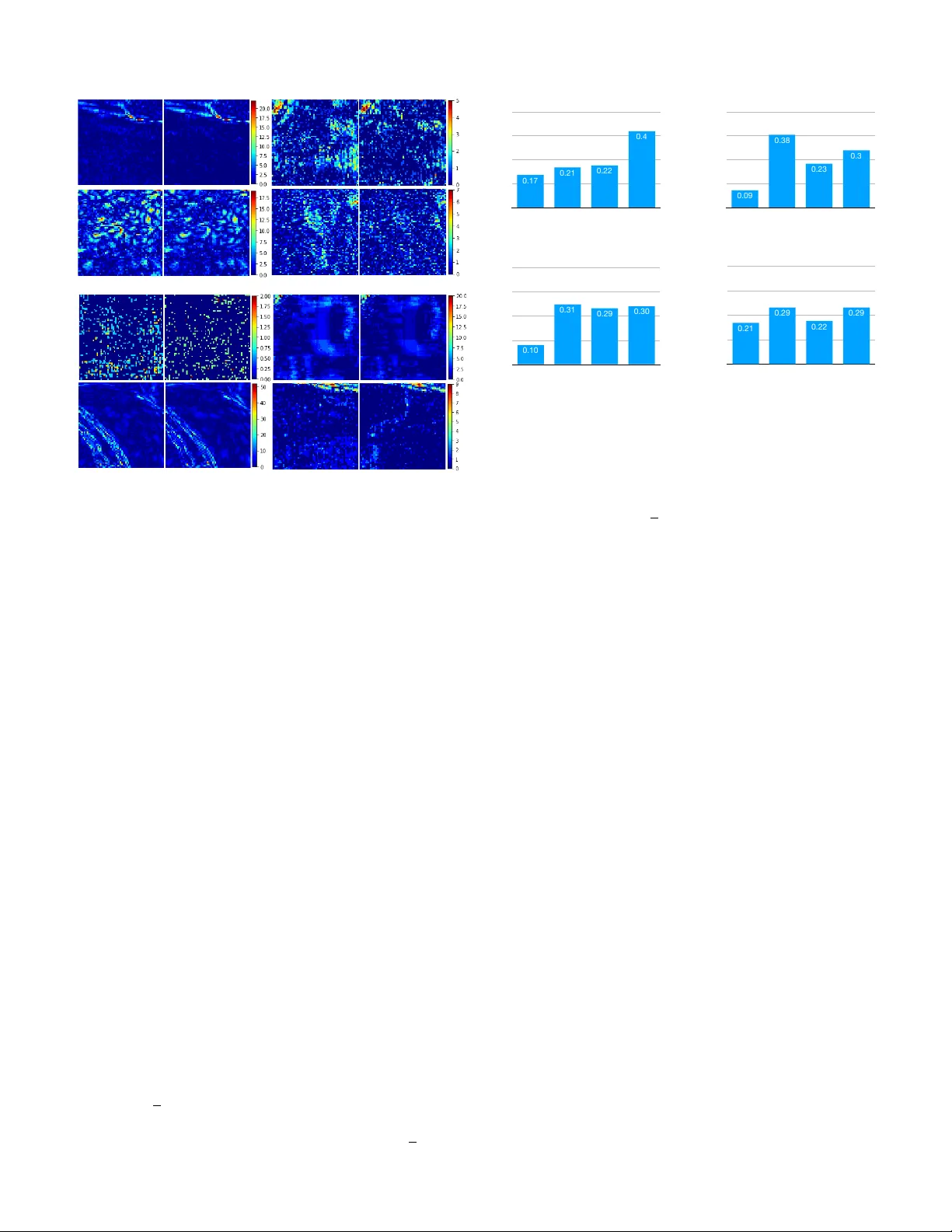
PREP ARED FOR IEEE TRANSA CTIONS ON 1 P artition-A ware Adapti v e Switching Neural Networks for Post-Processing in HEVC W eiyao Lin, Xiaoyi He, Xintong Han, Dong Liu, John See, Junni Zou, Hongkai Xiong, and Feng W u, F ellow , IEEE Abstract —This paper addresses neural netw ork based post- processing f or the state-of-the-art video coding standard, High Efficiency Video Coding (HEVC). W e first propose a partition- aware Con volution Neural Network (CNN) that utilizes the partition information pr oduced by the encoder to assist in the post-processing . In contrast to existing CNN-based approaches, which only take the decoded frame as input, the proposed approach considers the coding unit (CU) size information and combines it with the distorted decoded frame such that the artifacts introduced by HEVC are efficiently reduced. W e further introduce an adaptive-switching neural network (ASN) that consists of multiple independent CNNs to adaptively handle the variations in content and distortion within compressed- video frames, pr oviding further reduction in visual artifacts. Additionally , an iterative training procedur e is proposed to train these independent CNNs attentiv ely on different local patch-wise classes. Experiments on benchmark sequences demon- strate the effectiveness of our partition-aware and adaptive- switching neural networks. The project page can be found in http://min.sjtu.edu.cn/lwydemo/HEVCpostprocessing .html . Index T erms —High Efficiency V ideo Coding, Con volutional neural netw ork, Post-pr ocessing I . I N T RO D U C T I O N Recently , the fast de velopment of video capture and display devices has brought a dramatic demand for high definition (HD) contents. Thus, High Efficiency V ideo Coding (HEVC) [ 2 ] standard is developed by the Joint Collaborativ e T eam on V ideo Coding (JCT -VC). HEVC provides higher compression performance compared to the pre vious standard H.264/A VC by 50% of bitrate sa ving on average at a similar perceptual image quality [ 3 ]. Howe ver , HEVC videos still contain compression artifacts, such as blocking artifacts, ringing effects, blurring, etc. , making it of great importance to study on reducing the visual artifacts of the decoded videos. Over the past years, there has been a lot of work aiming at reducing the visual artifacts of decoded images [ 4 ]–[ 8 ] and videos [ 9 ]–[ 11 ]. Inspired by the great success achieved The basic idea of this paper appeared in our conference version [ 1 ]. In this version, we extend our approach by introducing an adaptive-switching scheme, carry out detailed analysis, and present more performance results. W . Lin, X. He, and H. Xiong are with the Department of Electronic Engineering, Shanghai Jiao T ong University , China (Email: { wylin, 515974418, xionghongkai } @sjtu.edu.cn). X. Han is with Huya Inc., China (Email: xintong@umd.edu). J. See is with the Faculty of Computing and Informatics, Multimedia Univ ersity , Malaysia (Email: johnsee@mmu.edu.my). J. Zou is with the Department of Computer Science and Engineering, Shanghai Jiao T ong University , China (Email: zou-jn@cs.sjtu.edu.cn). D. Liu and F . W u are with the School of Information Science and T echnology , University of Science and T echnology of China (Email: { dongeliu, fengwu } @ustc.edu.cn). Decoded Frame Post-processed Frame Artifact Reduction CNN D e co d e d F ra me En h a n ce d F ra me (PSN R i mp ro ve d ) Quality Enhancement CNN En h a n ce d F ra me (a) Decoded Frame Partition Information Mask Generation Exa mp l e o f ma sk Partition-aware CNN Post-processed Frame (b) Decoded Frame Patches Residual Heatmap (c) Switch Flag from bitstream, e.g. 3 CNN_0(L) CNN_1(L) CNN_2(L) Our proposed iterative training Adaptive-switching network CNN_3(G) (d) Figure 1. (a) Traditional single input methods; (b) Our partition-aware CNN; (c) Heatmap of residual; (d) Our adaptive-switching neural network. by deep learning techniques in computer vision and image processing tasks [ 12 ]–[ 14 ], many con v olutional neural netw ork based approaches [ 15 ]–[ 22 ] hav e been proposed to mitigate the visual artifacts in decoded images and videos. As for reducing the visual artifacts of HEVC compressed videos, [ 17 ]–[ 22 ] introduced a set of CNN-based filters which post-process HEVC compressed frames and obtain improved visual quality by suppressing artif acts. Ho we ver , most existing methods [ 17 ]–[ 19 ], [ 21 ], [ 22 ] only take the decoded patches as the input to the CNN and output the post-processed patches directly as shown in Fig. 1a , while no other prior information is taken into consideration explicitly . In this paper , we posit that partition information ( e.g. , 16 × 16, 8 × 8 [ 2 ], shown in Fig 1b ) could be used to effecti vely guide the post-processing performed by CNN. In practice, since the partition information is introduced by the block-wise processing and quantization of HEVC, it is related to the content of the frame and indicates the source of visual compression artifacts. Based on this intuition, we propose a nov el approach (shown in Fig. 1b ) that first deriv es a carefully designed mask from a frame’ s partition information, and then uses it to guide the post-processing of the decoded frame through a partition- aware CNN. Note that the partition information (e.g., 16 × 16, 8 × 8) is generated already by encoder [ 23 ]. As a result, the visual artifacts of HEVC-compressed videos can be more PREP ARED FOR IEEE TRANSA CTIONS ON 2 Selection CNN_0(L) CNN_1(L) CNN_2(L) CNN_3(G) O ri g i n a l Pa t ch Binarization Bi t s O u r p ro p o se d i t e ra t i ve t ra i n i n g p ro ce d u re D e co d e d Pa t ch Pa rt i t i o n I n f o rma t i o n Partition-aware CNN Mask Generation Feature Extraction Feature Extraction Mask-patch fusion Feature Enhancement&Reco nstruction Post-processed Patch Input Mask Input Patch Ad a p t i ve -sw i t ch i n g n e t w o rk p a ri t i o n -ma kse d CNNs (a) Selection CNN_0(L) CNN_1(L) CNN_2(L) CNN_3(G) Original Patch Binarization Bits Our proposed iterative training procedure Decoded Patch Partition Information Pa rt i t i o n -a w a re C N N Mask Generation Featur e Extraction Featur e Extraction Mask-patch fusion Featur e Enhancement&Reco nstruction Po st -p ro ce sse d Pa t ch Input Ma sk Input Pa t ch Adaptive-switching neural network partition-aware CNNs (b) Figure 2. The frame work of our proposed method. (a) Partition-aware CNN; (b) Adapti ve-switching scheme. effecti vely reduced under the same bit rate. Moreov er , the recent study [ 20 ] attempts to use two CNNs with dif ferent architectures to handle degradation v ariation in HEVC intra and inter coding. Though it has the specific architectures for HEVC intra- and inter -coding frames, the degradation variation within decoded frames ( e.g. , among patches) is neglected. Fig. 1c shows examples of patches and their corresponding residual heatmaps from one decoded frame. The residual is the absolute difference between the decoded and original frames (only Y -channel is shown). W e can see obvious difference among these three patches’ resid- ual heatmaps. This indicates different patches may need to be treated differently for post-processing. T o this end, we introduce an adaptiv e-switching scheme to handle degradation variation within decoded frames, which leads to further perfor - mance improv ement. Its framework in decoder side is shown in Fig. 1d . Patches are relayed to independent CNNs in an adaptiv e-switching neural network (ASN) based on flags read from the bitstream. The designed ASN consists of multiple CNNs, where we let CNN i(L) denote the local CNN with index i ( i ∈ [0 , 2] ) and CNN 3(G) denote the global CNN. Note that all local CNNs are trained by our proposed iterati ve training method to enable each of them focus more on the specific class of local patches and the global CNN is trained on the whole training dataset (see Section IV -A for more details). In summary , our contributions are three-fold: 1) W e develop a novel frame work that utilizes the partition information to guide the CNN-based post-processing in HEVC, where a mask deriv ed from a decoded frame’ s partition information is fused with this decoded frame through a partition-aware CNN to accomplish post- processing. Besides, under this framework, we system- atically in vestigate dif ferent mask generation and mask- frame fusion methods and find the best strategies. W e also demonstrate that our approach is general and can be integrated into the existing HEVC compressed-video post-processing methods to further improve their perfor- mances. 2) Our adapti ve-switching scheme utilizes multiple CNNs (one global and a set of local CNNs) to handle degra- dation variation of local patches within decoded frames and further reduce the visual artifacts. Moreov er , all local CNNs are trained by our carefully designed iterati ve training strategy , so that each of them concentrates on specific class of local patches. W e conduct experiments by applying this scheme and training method to demon- strate their ef fecti veness with dif ferent CNN architectures. 3) W e establish a large-scale dataset containing 202,251 training samples for encouraging training compressed- video post-processing models. This dataset will be made publicly av ailable to facilitate further research. The frameworks of our work. The frame works of the proposed partition-aware CNN and adapti ve-switching scheme are shown in Fig 2 . Our partition-a ware CNN, which is detailed in Section III , is shown in Fig 2a . For each patch in a decoded frame, we obtain its corresponding mask generated by the patch’ s partition information, and fed this information together with the patch into a partition-a ware CNN. Inside this CNN, the features of the mask and decoded patch are first extracted through two individual streams and then fused into one. The rest layers of the partition-aware CNN perform the feature enhancement, mapping, reconstruction, and output the post-processed patch with reduced artifacts. As for our adaptive-switching scheme (detailed in Sec- tion IV ) sho wn in 2b , each patch is post-processed by a bank of trained CNNs in the encoder side. These CNNs consist of three local CNNs ( CNN 0(L) , CNN 1(L) , CNN 2(L) ) and one global CNN ( CNN 3(G) ) . Then the CNN is chosen such that the difference (measured by PSNR [ 2 ]) between the post-processed patch and its original patch is smallest across all CNNs. This amounts to greedily choosing the CNN that generated the most similar one to original frame patch in terms of PSNR among all CNNs. The indices of chosen CNNs are directly written into bitstream after binarization. The rest of this paper is organized as follo ws. Section II revie ws related works. Sections III describes the proposed partition-aware CNN in detail. In Section IV , we describe the details of our proposed adaptive-switching scheme. Section V shows the experimental settings and results of our proposed partition-aware CNN and adaptive-switching scheme. Section VI concludes the paper . PREP ARED FOR IEEE TRANSA CTIONS ON 3 (a) Concatenation-based late fusion (b) Addition-based fusion. (c) Concatenation-based early fusion Figure 3. Different fusion methods to combine the decoded frame and mask. (a) Original frame with partition information (b) Local Mean-based mask (c) Boundary-based mask Figure 4. T wo examples of boundary-based mask and local mean-based mask. I I . R E L A T E D W O R K Over the past decades, a lot of works aiming to reduce visual artifacts hav e been proposed. Lie w et al. [ 4 ] proposed a wa velet-based deblocking algorithm to reduce artifacts of compressed images. Jancsary et al. [ 5 ] dev eloped a densely- connected tractable conditional random field to achieve JPEG images deblocking. Non-local means filter was applied to remov e quantization noise on blocks by W ang et al. in [ 7 ]. Recently , due to the impressiv e achiev ements of deep neural networks in computer vision and image processing tasks, many deep learning based methods are proposed to further reduce the visual artifacts of decoded images [ 15 ]–[ 18 ], [ 20 ]. More specifically , Dong et al. [ 15 ] de veloped an Artifacts Reduction CNN (ARCNN) built upon [ 24 ], which successfully reduces the JPEG compression artifacts. The proposed netw ork contains four con v olutional layers and takes the JPEG com- pressed image as input and outputs artifact-reduced decoded image directly . According to [ 15 ], ARCNN sho ws superior performance compared with the state-of-the-art conv entional methods. This inspires researches to focus on deep learning based methods for reducing visual artifacts. Following the similar line, [ 16 ] designed a Deep Dual-Domain network that takes the prior knowledge of the JPEG into consideration to remov e artifacts of JPEG compressed images. Similar to images, there are also a lot of works focusing on deep learning based artifact reduction for decoded videos [ 17 ], [ 18 ], [ 20 ]. Park and Kim [ 17 ] proposed an In-loop Filter CNN (IFCNN) based on SRCNN [ 24 ] to replace the Sample Adapti ve Offset (SA O) filter in HEVC. There are two in-loop filters in HEVC: deblocking filter and SA O filter . These in-loop filters are able to improve visual quality and decrease bit-rate of compressed videos and therefore improve coding efficienc y . IFCNN outperforms the HEVC reference mode (HM) with average 1.9% - 2.8% bit-rate reduction for Low Delay configuration, and av erage 1.6% - 2.6% bit-rate reduction for Random Access configuration. Slightly dif ferent from [ 17 ], Dai et al. [ 18 ] designed a VRCNN based on ARCNN [ 15 ] as a post-processing technique to further reduce the visual artifacts of decoded frames in HEVC. VRCNN can improve the visual quality of decoded frames without any increase in bit-rate and therefore also can impro ve the coding ef ficiency of HEVC in av erage 4.6% bit-rate re- duction for intra coding. T o further improv e coding ef ficiency , W ang et al. [ 19 ] proposed a deeper CNN called DCAD that has 10 conv olutional layers. The same model trained by intra- coding frames of HEVC are applied for both intra and inter coding during the test stage in [ 19 ]. Howe ver , since these works do not consider any prior information and only take decoded frame as input, they have limitations in handling complex de gradation introduced by HEVC. Recently , Y ang et al. [ 20 ] proposed QECNN that has specific architectures for HEVC intra- and inter - coding frames. This amounts to process I and P/B frames in HEVC with two separate models. But degradation variation within decoded frames is neglected and the potential of multiple CNNs can be further explored. In contrast to these existing methods, our proposed partition- aware CNN takes the partition information into consideration and a mask derived from it is fed into CNN. Besides, we propose an adaptiv e-switching scheme considering content and degradation variation within compressed-video frames, where patches in decoder side are relayed to independent CNNs in a greedy fashion. Compared with the previous methods, the degradation introduced by HEVC can be reduced more ef ficiently using our partition-aw are CNN. Furthermore, compared with methods based on a single CNN, artifacts can be further reduced with our adaptiv e-switching scheme. I I I . T H E PA RT I T I O N - A WAR E N E T W O R K This section will first discuss the ke y components of our partition-aware CNN – mask generation & mask-patch fusion strategies, and then gi ve details of partition-aware CNN with the specific mask generation & mask-patch fusion strategies. A. Mask generation and mask-frame fusion strate gies Since the block-wise transform and quantization are per- formed in HEVC during encoding, the quality degradation of compressed frames is highly related to the coding unit (CU) partition [ 2 ]. Thus, the partition information contains useful PREP ARED FOR IEEE TRANSA CTIONS ON 4 Element -vise sum BN ReLu Conv BN Conv Post- processed Frame Mask Decoded Frame Conv ReLu Conv BN … 8 residual blocks Mask-flow Residual Block Conv ReLu Conv BN … Conv ReLu Conv ReLu Conv 32 residual blocks Fusion Element -vise sum Element -vise sum Residual Block Original Frame Mean Square Error Figure 5. Our partition-aw are CNN. clues for eliminating the artifacts presented during encoding. Considering this, we design a mask based on the partition information of these CUs to guide the post-processing process. Mask generation. W e introduce 2 strategies to generate masks from an HEVC-encoded frame’ s partition information: • Local mean-based mask (MM). W e fill each partition block in a frame with the mean v alue of all decoded pixels inside this partition. An example of a generated mean-based mask is shown in Fig. 4b . As we can see that the dif ferent partition blocks are properly displayed in the mask. In this way , when we fuse it with the decoded frame during the post-processing process, it can ef fecti vely distinguish different partition modes and reduce the compression artifacts more effecti vely . • Boundary-based mask (BM). W e also introduce a boundary-based mask generation strategy . In this mask, the boundary pixels between partitions are filled with value 1 and the rest non-boundary pixels are filled with 0 (cf. Fig. 4c ). The width of the boundary is set to 2. Mask-frame fusion strategies. The mask is fed into CNN and integrated with its corresponding decoded frame to get the fused feature maps. W e also introduce 3 strate gies to fuse the information of a decoded frame and its corresponding mask: • Concatenate-based late fusion (CLF). W e extract the features of mask only using three conv olutional layers and integrate it into the network as shown in Fig. 3a . • Add-based fusion (AF). As shown in Fig. 3b , we first extract the feature maps of the mask using CNN and then combine it with the feature maps of the input frame using element-wise add layer . • Concatenate-based early fusion (CEF). W e concatenate the mask and frame as the input to the CNN. Then the two-channel input is fed to CNN directly (cf. Fig. 3c ). B. Details of partition-awar e con volutional neural network In Fig. 5 , we illustrate the architecture of the proposed partition-aware conv olutional neural network that integrates partition information with add-based fusion strategy to reduce the visual artifacts of compressed frames. Note that the frame- work of our proposed partition-a ware CNN is general. Besides the CNN structure in Fig. 5 , it can also be inte grated with other CNN structures for performing post-processing. According to 5 , the CNN contains tw o streams in the feature extracting stage so as to extract features for the decoded frame and its corresponding mask, respectively . Each residual block [ 25 ], [ 26 ] in the feature extracting stage has two con volutional layers with 3 × 3 kernels and 64 feature maps, followed by batch-normalization [ 27 ] layers and ReLU activ ation func- tions. Then, the feature maps of the mask and decoded frame are fused by the add-based fusion strategy and are fed to the rest three con volutional layers. These three layers are utilized for feature enhancement, mapping, reconstruction (as described by [ 15 ]), and finally outputting the post-processed frame with reduced artifacts. Moreov er , when training the network, the Mean Squared Error between the original raw frame and the CNN output is used as the loss function. Compared with the existing compressed video post- processing methods [ 18 ], [ 20 ], our network has tw o differ - ences: (1) W e introduce two stream inputs to include both the decoded frame and the partition information. (2) W e use residual architecture to perform the feature extraction. The deep residual stream can capture the feature of input in a more distinctiv e and stable way . I V . A D A P T I V E - S W I T C HI N G S C H E M E T o increase the diversity of the local representations, we propose an iterati ve training procedure to obtain local CNNs in the form of an adaptiv e-switching neural network. Besides, this scheme also aids in the artifact reduction of local patches of different classes. A. Iterative training The framework of this iterativ e procedure is shown in Fig. 6 . At the first step, the labels of all training patches are initialized by a specific initialization method with the number of classes set to three. Their corresponding pre-trained models at this initial step are also provided. For each iteration, each individual local CNN is fine-tuned from the model obtained from the pre vious iteration based on its corresponding patch PREP ARED FOR IEEE TRANSA CTIONS ON 5 Patches with labels 0 1 2 Local CNNs in ASN T raining data Initial Classification CNN_0(L) CNN_1(L) CNN_2(L) T raining Models from ! last iteration Performance Analysis Initialization Label refinement CNN_3(G) Pre-trained ! global CNN Figure 6. The frame work of our iterativ e training. class. W e obtain the final local CNNs when the training con- ver ges after a number of epochs. In the performance analysis step, the trained local CNNs and a pre-trained global CNN are used to generate new labels for all training patches. The pre-trained global CNN is fixed and used during performance analysis only . After label refinement, each training patch in the training set is assigned a ne w label. This procedure is repeated until the performance of adaptiv e-switching neural network con verges (with little further change) or the maximum number of iterations is reached. W e now discuss in detail the key components of our pro- posed scheme - initialization methods & the iterati ve process. 1) Initialization methods: Since we do not have the ground truth label for each patch, selecting a proper initialization method is ke y to effecti ve iterative training. W e introduce three initialization methods (as illustrated in Fig. 7 ): Random initialization, PSNR-based initialization method, and Cluster- based initialization method. • Random Initialization. In this method, the labels for all training patches are initialized at random. • PSNR-based initialization method. Using the PSNR of all training patches, we pick two thresholds that split the training patches into three quasi-equal parts. Then, we consider each part as one patch class of training data. Note that this initialization method is essentially based on the attributes of the residual in the pixel domain. • Cluster -based initialization method. This initialization method classifies the training data according to attributes of the residual in the frequency domain. As shown in Fig. 7 , we first compute the absolute residual between decoded and original patch, which is then transformed by DCT . After dimensionality reduction, the DCT co- efficients in zigzag-order (called feature vectors) are clustered to assign a label to each patch. Formally , we can define the Feature V ectors ( F V ) used to cluster as: F V ( X, Y ) = Z ig z ag ( D C T ( abs ( X − Y ))) (1) where X ∈ Q W × H is the decoded frame, Y ∈ Q W × H is the original frame, Q is the GF (2 8 ) finite field, abs ( · ) takes the absolute value of each element, D C T ( · ) is the DCT operation while Z ig z ag ( · ) flattens the matrix into vector in zigzag scan order . In essence, F V ( X , Y ) ∈ [ a i,j ] W H × 1 where a i,j ∈ [0 , 1] . Since a lot of DCT coefficients are zero, the dimensionality of the FVs is reduced by t-SNE [ 28 ]. Random Label Assignment PSNR Analysis Label Assignment Thresholds DCT T ransform Residual Computation Dimension Reduction Cluster Label Assignment Initial Classification Random Initialization PSNR-based Initialization Cluster -based Initialization T raining data Figure 7. Different initialization methods. W e compare these three initialization methods in Section V and visualize their respective classification results of different initialization methods at different iteration steps in Section V -D1 for better understanding their behaviors. 2) Iterative pr ocess.: W e utilize an iterati v e training process that updates and refines the classification of training data iterativ ely to accomplish the training of local CNNs in the adaptiv e-switching neural network. There are two stages in this process: pre-training and iterativ e update: • Pr e-training. These three local CNNs are pre-trained separately on three different subsets of the training data with the aim of learning good initial weights. The mean square error (MSE) loss is used during optimization. T o increase the div ersity of samples used in these CNNs, the subsets used in pre-training are carefully deri ved. W e first split the training data into fi ve subsets (similar to ho w it is done in a 5-fold cross-validation). Then the CNNs of adaptiv e-switching scheme at QP=37 are pre-trained using three randomly selected subsets from among the fiv e. • Iterativ e update . Let F ( X n ; Θ i ) represent the out- put of a CNN parameterized by Θ i for input X n . The trained local CNNs for the ( i − 1) - th iteration step are each parameterized by their respectiv e weights, i.e. Θ 0 ,i − 1 , Θ 1 ,i − 1 , Θ 2 ,i − 1 . Meanwhile, the pre-trained global CNN is fixed, with its parameters denoted as Θ 3 ,i − 1 at ( i − 1) - th step. In the performance analysis step sho wn in Fig. 6 , a new label for each training patch is generated for each i - th iteration using equation 2 : l best n = arg min j P S N R ( F ( X n ; Θ j,i − 1 ) , Y n ) (2) for j ∈ [0 , 3] where Y n is the corresponding original patch of the input training patch X n . After label refinement is completed, each training patch will be assigned a new label. Next, all local CNNs are fine-tuned again on the training set with updated patch labels. Note that each local CNN is only trained on one particular class of training patches (i.e., subset of patches with a particular patch label value). This procedure is repeated until the PREP ARED FOR IEEE TRANSA CTIONS ON 6 𝚫 PSNR 0.27 0.308 0.345 0.383 0.42 Number of iteration steps 1 2 3 4 5 6 7 8 9 10 Cluster -based Random Initializtion PSNR-based Figure 8. Conv ergence curve for the iterative process in our approach. x - axis: number of iteration steps; y -axis: gain of adaptiv e-switching neural network (measured by Y -channel PSNR impro vement over HM-16.0 baseline on v alidation set). Best viewed in color gain (PSNR improvement over HM-16.0 baseline) of the adaptiv e-switching neural network on the validation set con v erges or the maximum number of iterations is reached. Although the exact con ver gence of our iterative process is difficult to analyze due to the inclusion of label refinement, our experiments show that the gain of the adaptive-switching neural network stabilizes within 10 iteration steps for all three initialization methods, which implies the reliability of our approach. From the conv er gence curves shown in Fig. 8 , we can observe that the average ∆ PSNRs of our adaptive- switching neural network con ver ged quickly at levels of around 0.386, 0.403 and 0.406 dB PSNR improvements over HM-16.0 baseline for the random, PSNR-based and cluster- based initialization methods. W e note the following observations about our adaptive- switching scheme: 1) The local CNNs could focus on a small specific parts of a frame by way of the patches without resulting in over - fitting since the global CNN can ensure the lower bound of performance. 2) The scheme is independent of the architecture of sub- CNNs utilized 3) Flags corresponding to the trained CNNs can be easily binarized and written into bitstreams (2 bits for 4 cases). B. T est stage The framework of our proposed adapti ve-switching scheme is shown in Fig. 2b (encoder side) and Fig. 1d (decoder side). Encoder side. After all trained CNNs have been obtained using our proposed iterative training method, we proceed to the encoding procedure. In the encoder side (see Fig. 2b ), an input patch X n is post-processed by all trained CNNs separately . Then the F l ag n - th CNN is chosen such that the PSNR between F ( X n ; Θ F lag n ) and Y n is smallest across all trained CNNs. Formally , we define the flag of the chosen F l ag n - th CNN as: F l ag n = arg min j P S N R ( F ( X n ; Θ j ) , Y n ) (3) Figure 9. Example snapshots from our training dataset. where all notations are the same as in Equation ( 2 ). These flags indicating the indices of chosen CNNs for all patches, are written into the bitstream after binarization. Decoder side. In the decoder side, the flags are first obtained from the bitstream. For a patch X n , the CNN used to accom- plish post-processing is chosen according to the corresponding flag F l ag n . Hence, processing for each decoded frame is achiev ed by passing each patch through its selected CNN. Note that we do not know the PSNR between the post-processed patch and original patch since the original frame is unknown on the decoder side. V . E X P E R I M E N T S A. Dataset In order to encourage a more comprehensiv e validation process, we establish a large-scale dataset. The dataset is deriv ed from 600 video clips of various resolutions (i.e. 1920 × 1080 , 1280 × 720 , 832 × 480 pixels) with a frame rate of 30 f ps for all videos. Fig. 9 shows some snapshots of the video clips. All raw video clips are encoded by HM-16.0 at Low-delay P at QP=22, 27, 32, and 37. In each raw clip and its compressed clip, we randomly select 3 raw frames and their corresponding decoded frames to form 3 training frame pairs. For each frame pair , we further divide them into 64 × 64 non- ov erlapping sub-images, resulting in 202,251 sub-image pairs. W e use only the luminance channel (Y -channel) for training. B. Experimental Settings In our experiments, all models are implemented using T ensorFlow [ 29 ]. MSE is applied as the loss function for our proposed networks, and it is formally denoted as: L (Θ) = 1 N N X n =1 k F ( X n ; Θ) − Y n k 2 2 (4) with similar notations to earlier equations; X n is the input compressed frame, Θ is the learnable parameters of the whole network and Y n is the original frame. For the partition-aware CNN, we use a mini-batch size of 32. W e start with a learning rate of 1e-04, decaying by a power of 10 at the 20 th epoch, and terminating at the 40 th epoch. An individual CNN is trained for each QP . T o reduce training time, we first train the CNN at QP=37 from scratch and the other networks at QP=32, 27, 22 are fine-tuned from it. For all cases, the global CNN of the adaptive-switching scheme is directly trained on the entire training dataset while all local CNNs are trained using the iterati ve training method. PREP ARED FOR IEEE TRANSA CTIONS ON 7 T able I C O MPA R IS O N O F D I FFE R E N T M A SK A N D F U S I ON M E T HO D S O N Y - C H A NN E L ∆ P S N R ( D B ) OV E R H M - 1 6. 0 BA S E L IN E A T Q P = 2 7/ 3 7 U N DE R L P C O NFI G U R A T I O N . QP Class Sequence 1-in 2-in +BM +AF 2-in +MM+CLF 2-in +MM+CEF 2-in +MM +AF 27/37 A T raffic 0.3497 / 0.3064 0.3908 / 0.3679 0.3868 / 0.3592 0.3600 / 0.3317 0.3880 / 0.3943 PeopleOnStreet 0.4827 / 0.5592 0.5180 / 0.6367 0.5225 / 0.6382 0.4846 / 0.6087 0.4262 / 0.6410 Nebuta 0.4503 / 0.2679 0.4959 / 0.1994 0.5132 / 0.2491 0.4707 / 0.3000 0.3484 / 0.3200 SteamLocomotiv e 0.2902 / 0.1857 0.3160 / 0.1217 0.3268 / 0.1826 0.3113 / 0.1900 0.2643 / 0.2210 A verage 0.3932 / 0.3298 0.4302 / 0.3314 0.4373 / 0.3573 0.4067 / 0.3576 0.3567 / 0.3941 B Kimono 0.3859 / 0.3552 0.4184 / 0.3932 0.4165 / 0.3829 0.3860 / 0.3934 0.3878 / 0.4149 ParkScene 0.1940 / 0.1693 0.2232 / 0.1927 0.2208 / 0.1883 0.2002 / 0.1877 0.2263 / 0.1994 Cactus 0.2154 / 0.2288 0.2431 / 0.3130 0.2450 / 0.3005 0.2175 / 0.2704 0.2412 / 0.3374 BQT errace 0.1767 / 0.1836 0.2080 / 0.2950 0.2071 / 0.2754 0.1889 / 0.2881 0.2429 / 0.3791 BasketballDri ve 0.1586 / 0.1918 0.2010 / 0.3208 0.1978 / 0.3076 0.1557 / 0.2988 0.2225 / 0.3518 A verage 0.2261 / 0.2257 0.2587 / 0.3029 0.2575 / 0.2910 0.2297 / 0.2877 0.2641 / 0.3365 C RaceHorses 0.2557 / 0.2594 0.2793 / 0.2962 0.2807 / 0.2900 0.2530 / 0.2904 0.2699 / 0.2943 BQMall 0.1965 / 0.0954 0.2698 / 0.2465 0.2764 / 0.2280 0.2184 / 0.2700 0.3201 / 0.3554 PartyScene 0.1299 / 0.1052 0.1643 / 0.1728 0.1746 / 0.1538 0.1388 / 0.1890 0.2136 / 0.2715 BasketballDrill 0.2686 / 0.2228 0.3784 / 0.3401 0.3860 / 0.3230 0.3093 / 0.3228 0.4490 / 0.4699 A verage 0.2127 / 0.1707 0.2730 / 0.2639 0.2794 / 0.2487 0.2299 / 0.2681 0.3132 / 0.3478 D RaceHorses 0.3817 / 0.3090 0.4381 / 0.4212 0.4424 / 0.4094 0.3814 / 0.4130 0.3932 / 0.4060 BQSquare 0.1511 / -0.04 0.2269 / 0.2218 0.2216 / 0.1605 0.1795 / 0.2442 0.3345 / 0.4986 BlowingBubbles 0.1918 / 0.1250 0.2463 / 0.2190 0.2431 / 0.1976 0.1993 / 0.2181 0.2593 / 0.2578 BasketballPass 0.2465 / 0.1882 0.3273 / 0.3510 0.3233 / 0.3200 0.2707 / 0.3555 0.3739 / 0.4007 A verage 0.2428 / 0.1459 0.3097 / 0.3033 0.3076 / 0.2719 0.2577 / 0.3077 0.3402 / 0.3908 E FourPeople 0.4619 / 0.4426 0.5190 / 0.5545 0.5264 / 0.5448 0.4551 / 0.5312 0.5258 / 0.6244 Johnny 0.2996 / 0.3496 0.5190 / 0.5545 0.2604 / 0.4682 0.3118 / 0.4531 0.4285 / 0.5402 KristenAndSara 0.3395 / 0.3927 0.3967 / 0.5634 0.3563 / 0.5230 0.3748 / 0.5190 0.4298 / 0.5942 A verage 0.3670 / 0.3950 0.4333 / 0.5317 0.3810 / 0.5120 0.3806 / 0.5011 0.4614 / 0.5863 A verage 0.2813 / 0.2449 0.3322 / 0.3352 0.3264 / 0.3251 0.2934 / 0.3338 0.3373 / 0.3986 Overall, it takes about 26 hours to train a single partition- aware CNN from scratch (on 1 GeForce GTX 1080T i GPU), and 70 hours to train the adapti ve-switching neural network from scratch (on 4 GeForce GTX 1080T i GPUs). Note that our adaptiv e-switching scheme is independent of the architecture of these sub-CNNs, hence allowing the flexibility of plugging in other existing CNN-based models. In our experiments, we also compare the performance of the proposed adaptive-switching scheme with different CNN architectures. For the e valuation, we tested our trained model on 20 benchmark sequences (not included in our training set) from the Common T est Conditions of HEVC [ 30 ] under the same configuration as with training, Low-delay P [ 31 ]. Perfor- mance is measured by PSNR improv ement ( ∆ PSNR) and the Rate-distortion performance measured by the Bjontegaard Distortion-rate sa vings (BD-rate savings, calculated at QP=22, 27, 32, 37) [ 32 ] over the standard HEVC test model HM-16.0 (i.e., HM-16.0 baseline). Basically , a larger PSNR improve- ment or a larger BD-rate saving indicate that more visual artifacts are reduced. Note that both in-loop filters (deblocking filter & SA O filter) are turned on in HM-16.0. For a more in-depth ev aluation of our methods, performances on other configurations (Lo w- delay B, Random access, All intra) and color channels are also obtained for the purpose of comparing against our methods. Moreov er , in order to obtain fair comparison, all methods in T able I are trained using the same dataset (i.e., our dataset), and ev aluated under the same settings. T able II C O MPA R IS O N O F D I FFE R E N T M A SK A N D F U S I ON M E T HO D S O N B D - RATE ( Y , % ) O VE R H M -1 6 . 0 B AS E L I NE U N D ER L P C O NFI G U R A T I O N Class Sequence 1-in 2-in +BM +AF 2-in +MM +CLF 2-in +MM +CEF 2-in +MM +AF A T raffic -9.27 -11.27 -11.25 -10.58 -11.35 PeopleOnStreet -9.84 -11.48 -11.54 -10.90 -10.36 Nebuta -6.23 -8.03 -8.13 -7.91 -7.85 SteamLocomotiv e -10.22 -11.79 -12.30 -11.84 -10.6 A verage -8.89 -10.64 -10.81 -10.31 -10.04 B Kimono -9.49 -11.19 -11.14 -10.64 -10.91 ParkScene -5.4 -6.74 -6.75 -6.38 -6.92 Cactus -8.13 -10.50 -10.43 -9.04 -10.53 BQT errace -7.25 -9.45 -9.29 -6.61 -11.07 BasketballDri ve -6.42 -10.06 -10.14 -8.85 -11.10 A verage -7.34 -9.59 -9.55 -8.30 -10.10 C RaceHorses -5.57 -6.6 -6.61 -6.23 -6.45 BQMall -4.01 -6.62 -6.75 -6.03 -7.62 PartyScene -2.48 -3.79 -3.85 -3.55 -4.84 BasketballDrill -5.71 -9.11 -9.20 -8.12 -10.65 A verage -4.44 -6.53 -6.60 -5.98 -7.39 D RaceHorses -6.66 -8.29 -8.32 -7.66 -7.58 BQSquare -2.48 -5.66 -5.58 -5.09 -8.48 BlowingBubbles -4.12 -6.08 -6.00 -5.41 -6.33 BasketballPass -4.49 -7.02 -6.98 -6.32 -7.73 A verage -4.44 -6.76 -6.72 -6.12 -7.53 E FourPeople -10.69 -13.47 -13.55 -12.69 -13.91 Johnny -10.40 -15.64 -11.67 -14.17 -17.22 KristenAndSara -9.5 -12.94 -11.43 -12.43 -13.78 A verage -10.20 -14.02 -12.22 -13.10 -14.97 A verage -6.92 -9.29 -9.05 -8.63 -9.76 C. Results of partition-awar e CNNs under various strate gies 1) P erformance of visual artifact r eduction: T able I com- pares the performances of dif ferent mask generation and mask- frame fusion strategies described in Fig. 4 and Fig. 3 in terms of the Y -channel PSNR improv ement over HM-16.0 baseline PREP ARED FOR IEEE TRANSA CTIONS ON 8 T able III C O MPA R IS O N O F D I FFE R E N T I N IT I A L IZ ATI O N M E T H OD S O N Y - CH A N N EL ∆ P S N R ( D B ) O VE R H M -1 6 . 0 B A SE L I NE AT Q P = 37 U N D ER L P C O NFI G U R A T I O N . QP Class Sequences ASN@4 S ? Random PSNR-based Cluster-based 37 A T raffic 0.3048 0.3291 0.3366 PeopleOnStreet 0.5640 0.5978 0.6139 Nebuta 0.2814 0.3110 0.3232 SteamLocomotiv e 0.1937 0.2059 0.2148 A verage 0.3360 0.3610 0.3721 B Kimono 0.3722 0.4020 0.4162 ParkScene 0.1752 0.1900 0.1929 Cactus 0.2473 0.2827 0.2994 BQT errace 0.2096 0.2965 0.2995 BasketballDri ve 0.2499 0.3003 0.3036 A verage 0.2509 0.2943 0.3023 C RaceHorses 0.2693 0.2950 0.2984 BQMall 0.2198 0.2851 0.2761 PartyScene 0.1581 0.2110 0.2119 BasketballDrill 0.2650 0.3282 0.3365 A verage 0.2281 0.2798 0.2807 D RaceHorses 0.3725 0.4126 0.4170 BQSquare 0.2514 0.3529 0.3361 BlowingBubbles 0.1722 0.2093 0.2089 BasketballPass 0.2186 0.2926 0.3228 A verage 0.2537 0.3169 0.3212 E FourPeople 0.4372 0.4909 0.5393 Johnny 0.3748 0.4328 0.4645 KristenAndSara 0.4556 0.5214 0.5314 A verage 0.4225 0.4817 0.5118 A verage 0.2896 0.3374 0.3471 ( ∆ PSNR). In T able I , 1-in represents a single-input baseline approach where the mask-flo w input is omitted from the framew ork (Fig. 5 ); 2-in+MM+AF represents our partition- aware CNN using the local mean-based mask and add-based fusion strategy . From T able I , we can observe that: • When looking at dif ferent mask generation strategies, the boundary-based mask strategy (2-in+BM+AF) provides 0.33 dB PSNR improv ement that is similar to the local mean-based mask (2-in+MM+AF) at QP=27. Ho wev er , its performance at QP=37 is lo wer than 2-in+MM+AF by 0.06 dB. This is because only marking boundary pixels in a mask is slightly less effecti ve in highlighting the partition modes in a frame across different QPs. • As for mask-frame fusion strategies, the add-fusion strat- egy (2-in+MM+AF) can obtain large PSNR improve- ments of 0.40 dB at QP=37 and 0.34 dB at QP=27. This shows the effecti veness of the proposed fusion strategy . Comparati v ely , the concatenate-based late fu- sion (2-in+MM+CLF) and early-fusion (2-in+MM+CEF) strategies obtain smaller gains at both QP=27, 37. This is probably because these fusion strategies are less com- patible with the CNN model used in this paper . • The best performance is obtained when using local mean- based mask and add-fusion (2-in+MM+AF), which can obtain over 0.15 dB at QP=37 improvement o ver single- input method. Similar results can be found at QP=27. This indicates that when strategies are properly selected, introducing partition information is indeed useful to re- duce the visual artifacts of compressed videos. • Our baseline single-input method ( 1-in ) can also obtain satisfactory results. This implies that the baseline CNN 0 0.15 0.3 0.45 0.6 Class G Class L0 Class L1 Class L2 0.22 0.39 0.36 0.23 0.11 0.27 0.28 0.23 0.35 0.60 0.36 0.38 0.24 0.44 0.27 0.38 0.21 0.44 0.39 0.27 0.15 0.35 0.34 0.27 T ra ffi c, with CNN_3(G) only T ra ffi c, with ASN FourPeople, with CNN_3(G) only FourPeople, with ASN Overall, with CNN_3(G) only Overall, with ASN Figure 10. A verage Y -channel PSNR improv ement over HM-16.0 baseline of different classes of patches post-processed by ASN@4 S ? and its CNN 3(G) only at QP=37. Best viewed in color . T able IV N OTA T I O NS O F T H E C N N S U S E D I N T H E E X PE R I ME N T S O F O U R A DA P TI V E - SW I T C HI N G S C H E ME Original name Description Notation VRCNN [ 18 ] A shallow model proposed by [ 18 ] S VRCNN+MM+AF A partition-aw are shallo w model, which integrates our partition-aware-based approach into the existing VRCNN method S ? 1-in Our proposed single-input baseline without mask-flow input D 2-in+MM+AF A partition-aw are deep model of 1-in D ? model used in our approach is effecti ve in handling the visual information of the input decoded frames. 2) Rate-distortion performance: W e also compare the BD- rate saving of dif ferent mask and fusion methods ov er HM- 16.0 in T able II . Comparisons between these methods can be summarized as follows: (1) The local mean-based mask ( 2-in+MM+AF ) achie ves 0.47% BD-rate saving more than the boundary-based mask strategy ( 2-in+BM+AF ); (2) The concatenate-based late-fusion ( 2-in+MM+CLF ) and early- fusion ( 2-in+MM+CEF ) strategies obtain 9.05% and 8.63% BD-rate saving, which both are lower than the local mean- based mask ( 2-in+MM+AF ); (3) Our approach using local mean-based mask and add-fusion ( 2-in+MM+AF ) is able to achiev e up to 9.76% BD-rate saving ov er all test sequences. This again validates the effecti veness of introducing partition information when strate gies are properly selected. These ob- servations are also consistent with the PSNR improv ement measure. D. Results of our adaptive-switching scheme As shown in T able IV , the follo wing architectures are included in our comparativ e experiments: (1) A shallo w model VRCNN [ 18 ] denoted by S ; (2) A deep model, which is our proposed 1-in denoted by D ; (3) A partition-aware shallow model, VRCNN+MM+AF , which integrates our proposed par- tition a wareness into the e xisting VRCNN [ 18 ] method, which is denoted by S ? , and (4) Our partition-aware deep model, 2- in+MM+AF which is denoted by D ? . 1) Comparison of various initialization methods: T able III shows the Y -channel PSNR impro vement ov er HM-16.0 base- line for the three different initialization methods described in PREP ARED FOR IEEE TRANSA CTIONS ON 9 Class G Post-processed Residual Input Residual Post-processed Residual Input Residual Class L0 Class L1 Class L2 Figure 11. Examples of dif ferent classes of patches and corresponding for ASN@4 S ? with Cluster-based initialization method at the final iteration step. Best vie wed in color . Section IV -A . T o demonstrate this, we choose the ASN@4 S ? approach, which is our adaptive-switching neural network (ASN) with four sub-CNNs that are of the partition-aw are shallow model S ? . W e make the following observations: • Our approach with Cluster -based and PSNR-based initial- ization methods outperforms the Random method ov er all test sequences at QP=37. Obviously , the random initial- ization method is not able to provide a reasonable initial classification and thus resulted in a lo wer performance compared with the other two methods. • Our approach with Cluster -based initialization slightly outperforms that with the PSNR-based initialization by only 0.01dB. Specifically , the PSNR measure is propor- tional to the MSE loss function used and this led to a reasonably competiti ve result from the PSNR-based method. Howe ver , the Cluster-based method may be able to better capture the patch features in the frequency domain, achieving mar ginally better initial classification. Therefore, we decided to choose this initialization method for the rest of experiments in this paper . T o provide a control experiment on our choice of approach, we demonstrate that the iterativ e training process plays a major role for the case of our adaptive switching network, and this is consistent across all individual patch classes. Fig. 10 shows the av erage Y -channel PSNR improv ement of each class of patches post-processed by ASN@4 S ? with Cluster-based initialization method, and how it matches up against a single global CNN 3(G) . Each group of v ertical bars indicate the class of patches to be post-processed, e.g. Class G means that this class of patches are post-processed by CNN 3(G) on the decoder side when ASN is applied. As we can observe, 0.000 0.125 0.250 0.375 0.500 CNN_3(G) CNN_0(L) CNN_1(L) CNN_2(L) 0.4 0.22 0.21 0.17 (a) ASN@4 S 0.000 0.125 0.250 0.375 0.500 CNN_3(G) CNN_0(L) CNN_1(L) CNN_2(L) 0.3 0.23 0.38 0.09 (b) ASN@4 D 0.000 0.125 0.250 0.375 0.500 CNN_3(G) CNN_0(L) CNN_1(L) CNN_2(L) 0.30 0.29 0.31 0.10 (c) ASN@4 S ? 0.000 0.125 0.250 0.375 0.500 CNN_3(G) CNN_0(L) CNN_1(L) CNN_2(L) 0.29 0.22 0.29 0.21 (d) ASN@4 D ? Figure 12. Usage rate for adaptiv e-switching scheme with different CNN architectures. x -axis: model name in ASN; y -axis: usage rate during test at QP=37. the PSNR improvement achieved by ASN@4 S ? is lar ger than that achiev ed by its CNN 3(G) for each patch class for the T raffic sequence, F ourP eople sequence and ov erall across all benchmark sequences. Fig. 11 shows some examples of each class of patches. For each patch, we display the heatmap of residual between decoded patch and its ground truth (called input residual), and the heatmap of residual between post- processed patch and its ground truth (called post-processed residual). W e can see that the post-processed residual is less intensiv e than its corresponding input residual in all patch classes. 2) Comparison of various CNN arc hitectur es for the adaptive-switching neur al network: T ables V and VI compare the Y -channel PSNR improvement and BD-rate saving of adaptiv e switching network with different CNN architectures ov er HM-16.0 baseline. The follo wing adaptiv e-switching neu- ral networks are compared: (1) ASN@4 S , which means using the shallow model S [ 18 ] for all CNN architectures in the adaptiv e switching network; (2) ASN@4 D , which is similar to ASN@4 S but using the deep model D ; (3) ASN@4 S ? , where each CNN employs the partition-aw are shallow model S ? ; (4) ASN@4 D ? , where each CNN uses the partition-aware deep model D ? and; (5) ASN@ D ? + 3 S ? , which represents a hybrid combination of the global CNN based on the deep model D ? while all local CNNs use the shallow model S ? [ 18 ]. W e discuss the performance of the compared methods based on PSNR improvement and rate-distortion: • PSNR improv ement performance. From T able V we can observe that: (1) Our full method, ASN@4 D ? achiev es the highest PSNR improvement (0.47 dB) over HM-16.0 baseline at QP=37. When compared with its corresponding single-CNN-based method, D ? i.e., 2- in+MM+AF from T able I , it obtains a further 0.07 dB PSNR improvement. Results for QP=27 are of similar nature; (2) Comparing between the results of ASN@4 S and ASN@4 S ? , we find that the partition-aw are (latter) PREP ARED FOR IEEE TRANSA CTIONS ON 10 T able V C O MPA R IS O N O F A S N W I T H D I FFE R E N T C N N A R C H IT E C T UR E S O N Y - C H A NN E L ∆ P S N R AT Q P =2 7 , 3 7 U N D ER L P C O NFI G U R A T I O N . QP Class Sequence ASN@4 S ASN@4 S ? ASN@4 D ASN@4 D ? ASN@ D ? +3 S ? 27 / 37 A T raffic 0.3192 / 0.2907 0.3581 / 0.3366 0.4269 / 0.4437 0.4558 / 0.4579 0.4448 / 0.4106 PeopleOnStreet 0.4234 / 0.4670 0.5004 / 0.6139 0.5611 / 0.6995 0.6088 / 0.7286 0.6010 / 0.6781 Nebuta 0.4148 / 0.2401 0.5123 / 0.3232 0.5259 / 0.3594 0.5727 / 0.3829 0.5736 / 0.3321 SteamLocomotiv e 0.2831 / 0.1844 0.3324 / 0.2148 0.3484 / 0.2639 0.3742 / 0.2832 0.3728 / 0.2515 A verage 0.3601 / 0.2955 0.4258 / 0.3721 0.4656 / 0.4416 0.5029 / 0.4631 0.4980 / 0.4181 B Kimono 0.3377 / 0.3182 0.3938 / 0.4162 0.4496 / 0.4835 0.4860 / 0.4998 0.4802 / 0.4742 ParkScene 0.1770 / 0.1684 0.2064 / 0.1929 0.2342 / 0.2174 0.2690 / 0.2344 0.2649 / 0.2144 Cactus 0.1942 / 0.2315 0.2307 / 0.2994 0.2609 / 0.3882 0.2862 / 0.4044 0.2776 / 0.3596 BQT errace 0.1859 / 0.2232 0.2203 / 0.2995 0.2553 / 0.4154 0.2878 / 0.4328 0.2768 / 0.3310 BasketballDri ve 0.1370 / 0.2100 0.1813 / 0.3036 0.2425 / 0.4112 0.2723 / 0.4297 0.2477 / 0.3708 A verage 0.2064 / 0.2303 0.2465 / 0.3023 0.2885 / 0.3831 0.3203 / 0.4002 0.3094 / 0.3500 C RaceHorses 0.2322 / 0.2361 0.2734 / 0.2984 0.2932 / 0.3347 0.3267 / 0.3583 0.3126 / 0.3230 BQMall 0.1903 / 0.2067 0.2443 / 0.2761 0.3376 / 0.3837 0.3647 / 0.4200 0.3240 / 0.3293 PartyScene 0.1295 / 0.1404 0.1774 / 0.2119 0.2166 / 0.2881 0.2463 / 0.3120 0.2370 / 0.2385 BasketballDrill 0.2053 / 0.2434 0.3145 / 0.3365 0.4905 / 0.5348 0.5211 / 0.5549 0.4896 / 0.4455 A verage 0.1894 / 0.2067 0.2524 / 0.2807 0.3345 / 0.3853 0.3647 / 0.4113 0.3408 / 0.3341 D RaceHorses 0.3229 / 0.3278 0.4139 / 0.4170 0.4561 / 0.456 0.4974 / 0.4886 0.4844 / 0.4532 BQSquare 0.1543 / 0.2232 0.2460 / 0.3361 0.3387 / 0.5286 0.3563 / 0.5196 0.3223 / 0.3621 BlowingBubbles 0.1515 / 0.1646 0.2040 / 0.2089 0.2787 / 0.2754 0.3126 / 0.2960 0.2987 / 0.2456 BasketballPass 0.1932 / 0.2230 0.2681 / 0.3228 0.4005 / 0.4558 0.4324 / 0.4865 0.4063 / 0.3934 A verage 0.2055 / 0.2346 0.2830 / 0.3212 0.3685 / 0.4289 0.3997 / 0.4477 0.3779 / 0.3636 E FourPeople 0.4001 / 0.4207 0.4763 / 0.5393 0.5942 / 0.7027 0.6247 / 0.7350 0.5981 / 0.6496 Johnny 0.2862 / 0.3624 0.3428 / 0.4645 0.4542 / 0.6493 0.4913 / 0.6515 0.4653 / 0.5509 KristenAndSara 0.3517 / 0.4488 0.3967 / 0.5314 0.4686 / 0.7162 0.4912 / 0.7290 0.4733 / 0.6298 A verage 0.3460 / 0.4106 0.4052 / 0.5118 0.5056 / 0.6894 0.5357 / 0.7052 0.5122 / 0.6101 A verage 0.2545 / 0.2665 0.3146 / 0.3471 0.3817 / 0.4504 0.4139 / 0.4702 0.3975 / 0.4022 T able VI C O MPA R IS O N O F A S N W I T H D I FFE R E N T C N N A R C H IT E C T UR E S O N B D - R ATE ( Y , % ) O VE R H M -1 6 . 0 B A SE L I NE U N D ER L P C O NFI G U R A T I O N . Class Sequence ASN@ 4 S ASN@ 4 S ? ASN@ 4 D ASN@ 4 D ? ASN@ D ? +3 S ? A T raffic -8.83 -9.86 -11.73 -12.54 -12.14 PeopleOnStreet -9.33 -10.79 -11.54 -12.51 -12.66 Nebuta -7.14 -8.84 -8.58 -12.63 -9.61 SteamLocomotiv e -10.43 -12.16 -12.90 -14.39 -13.71 A verage -8.93 -10.41 -11.19 -13.02 -12.03 B Kimono -9.26 -10.58 -11.74 -12.60 -12.48 ParkScene -5.25 -6.04 -6.64 -7.89 -7.47 Cactus -8.04 -9.64 -10.75 -11.27 -11.64 BQT errace -7.97 -9.66 -11.29 -12.35 -11.85 BasketballDri ve -6.76 -8.89 -11.04 -11.58 -11.68 A verage -7.46 -8.96 -10.29 -11.14 -11.02 C RaceHorses -5.45 -6.39 -6.61 -7.51 -7.20 BQMall -4.48 -5.84 -7.43 -8.15 -7.55 PartyScene -2.86 -3.90 -4.63 -5.14 -5.04 BasketballDrill -5.30 -7.61 -11.08 -12.24 -11.19 A verage -4.52 -5.93 -7.44 -8.26 -7.75 D RaceHorses -6.16 -7.70 -8.08 -9.24 -8.82 BQSquare -3.99 -6.07 -8.24 -8.47 -7.66 BlowingBubbles -3.65 -4.84 -6.42 -7.33 -6.83 BasketballPass -3.70 -5.14 -7.52 -8.18 -7.70 A verage -4.37 -5.94 -7.56 -8.31 -7.75 E FourPeople -9.58 -11.41 -14.00 -14.44 -14.34 Johnny -10.61 -12.73 -16.72 -17.35 -17.01 KristenAndSara -9.90 -11.45 -13.62 -13.64 -13.75 A verage -10.03 -11.86 -14.78 -15.14 -15.03 A verage -6.94 -8.48 -10.03 -10.97 -10.52 A verage(corresp. single-CNN-based method) -3.57 -6.88 -6.92 -9.76 \ method outperforms the former method by 0.08 dB at QP=37 and 0.06 dB at QP=27. Interestingly, the ASN@4 D ? also marginally outperforms ASN@4 D ; (3) The hybrid combination method ASN@ D ? +3 S ? can also obtain satisfactory results for QP=27, higher than all other methods except for ASN@4 D ? . • Rate-distortion performance. As mentioned in IV -B , the flags indicating the indices of CNNs for each patch are written into the bitstream. Thus, it is necessary to ev aluate the rate-distortion performance of the proposed methods. T o this end, we further compare these methods in terms of BD-rate saving over HM-16.0 baseline. As shown in VI , we obtained some meaningful findings: (1) All adapti ve-switching neural netw orks outperform single-CNN-based methods - each of them can achiev e higher BD-rate saving than its corresponding single- CNN-based method. This demonstrates the effecti veness of our adaptiv e-switching scheme. Interestingly , the gap between ASN@4 D ? and D ? is smaller than that between ASN@4 S ? and S ? . There is less room for further per- formance improvement since the performance of D ? is already quite high (9.76%); (2) ASN@4 S can obtain a 6.94% BD-rate saving over HM-16.0 baseline. Since the CNNs used in ASN are deeper and more complex, the proposed ASN@4 D achie ves 10.49% BD-rate saving that is clearly better than ASN@4 S ; (3) ASN@4 S ? integrates our partition-aw are-based approach and outperforms the original approach (ASN@4 S ) by 1.54% BD-rate savings. The similar trend is found when comparing between the two deep model based methods. (4) The hybrid combination method achieves better results than their homogeneous counterparts – ASN@4 S , ASN@4 S ? & ASN@4 D . Since its time complexity on the decoder side is lower than that of ASN@4 D ? , the ASN@ D ? +3 S ? presents a practical version that is faster but still obtains satisfactory results. Moreov er , Fig. 12 further shows the usage rate of our PREP ARED FOR IEEE TRANSA CTIONS ON 11 T able VII C O MPA R IS O N O F D I FFE R E N T M E TH O D S O N B D - R ATE ( % ) S A V I N G OV E R H M - 1 6. 0 B AS E L IN E U N D ER D I FF ER E N T C O N FIG U R A T I O N S . Conf. Seq. VRCNN [ 18 ] QECNN-P [ 20 ] DRN [ 21 ] VRCNN+MM+AF DRN+MM+AF Our 2-in+MM+AF ( D ? ) Our ASN@4 D ? Y U V Y U V Y U V Y U V Y U V Y U V Y U V LP Class A -7.10 -2.41 -1.97 -8.43 -3.21 -2.78 -8.66 -3.58 -3.11 -9.00 -3.89 -3.48 -8.80 -4.42 -4.10 -10.04 -6.04 -5.72 -12.02 -6.63 -6.33 Class B -4.57 -4.13 -5.44 -6.39 -5.25 -7.21 -6.65 -5.91 -7.19 -7.28 -6.52 -8.30 -8.12 -6.99 -8.96 -10.10 -9.48 -11.94 -11.14 -10.64 -13.56 Class C -0.21 -2.73 -4.12 -2.81 -3.92 -5.59 -3.55 -4.45 -6.19 -4.05 -5.11 -7.03 -4.85 -5.34 -7.06 -7.39 -8.56 -11.07 -8.26 -9.66 -12.51 Class D 0.49 -1.88 -2.66 -2.52 -2.90 -3.70 -3.64 -3.32 -4.37 -4.16 -3.74 -4.86 -5.47 -4.38 -5.73 -7.53 -6.76 -8.36 -8.31 -8.23 -8.21 Class E -7.11 -11.25 -12.24 -9.47 -13.21 -14.02 -9.37 -13.16 -14.00 -10.79 -14.42 -15.08 -11.97 -15.08 -15.51 -14.97 -17.70 -17.75 -15.14 -18.52 -18.41 A verage -3.57 -4.13 -4.95 -5.77 -5.30 -6.32 -6.24 -5.72 -6.63 -6.88 -6.34 -7.41 -7.65 -6.84 -7.94 -9.76 -9.30 -10.68 -10.97 -10.34 -11.56 LB Class A -4.83 -1.13 -0.76 -5.85 -1.80 -1.45 -6.13 -2.27 -1.89 -6.43 -2.56 -2.23 -6.96 -3.03 -2.88 -7.74 -5.17 -4.88 -9.28 -5.57 -5.31 Class B -2.26 -2.68 -3.90 -3.92 -3.68 -5.57 -4.30 -4.45 -5.59 -4.73 -5.00 -6.64 -5.49 -5.40 -7.22 -7.58 -8.33 -10.68 -8.33 -9.21 -11.95 Class C 0.46 -2.07 -3.39 -2.05 -3.19 -4.78 -2.89 -3.75 -5.39 -3.27 -4.36 -6.16 -4.54 -5.12 -7.14 -6.86 -7.86 -10.20 -7.46 -8.87 -11.50 Class D 1.18 -1.55 -2.25 -1.89 -2.54 -3.24 -3.04 -2.97 -3.92 -3.45 -3.38 -4.35 -4.77 -3.93 -5.18 -7.31 -6.37 -7.98 -7.67 -6.85 -9.14 Class E -5.57 -10.52 -11.38 -7.78 -12.36 -13.03 -7.80 -12.30 -13.06 -9.05 -13.50 -14.04 -10.22 -14.08 -14.47 -13.04 -16.80 -16.73 -13.52 -17.56 -17.29 A verage -2.04 -3.20 -3.96 -4.11 -4.28 -5.24 -4.66 -4.76 -5.60 -5.17 -5.33 -6.31 -6.16 -5.88 -7.02 -8.23 -8.48 -9.79 -8.99 -9.20 -10.77 RA Class A -4.64 -0.42 -0.03 -5.60 -1.06 -0.68 -5.83 -1.68 -1.28 -6.15 -1.98 -1.64 -6.63 -2.49 -2.31 -7.36 -5.13 -4.81 -8.89 -5.39 -5.05 Class B -2.11 -1.39 -2.33 -3.69 -2.29 -3.82 -4.11 -3.28 -4.00 -4.54 -3.66 -4.90 -5.35 -4.04 -5.47 -7.53 -7.81 -9.88 -8.29 -8.23 -10.57 Class C 0.63 -1.48 -2.65 -1.77 -2.59 -4.03 -2.61 -3.27 -4.72 -2.97 -3.87 -5.45 -4.19 -4.67 -6.47 -6.48 -7.84 -10.14 -7.11 -8.72 -11.33 Class D 1.73 -0.74 -1.43 -1.30 -1.56 -2.33 -2.59 -2.22 -3.23 -2.88 -2.65 -3.58 -4.24 -3.20 -4.50 -6.95 -6.04 -7.88 -7.26 -7.32 -7.25 Class E -4.81 -9.48 -10.19 -6.85 -11.01 -11.46 -7.03 -11.19 -11.84 -8.15 -12.21 -12.67 -9.18 -12.52 -12.80 -12.54 -16.01 -15.75 -12.29 -16.05 -15.79 A verage -1.71 -2.30 -2.93 -3.68 -3.27 -4.08 -4.29 -3.93 -4.62 -4.76 -4.45 -5.26 -5.73 -4.96 -5.94 -7.92 -8.16 -9.40 -8.57 -8.75 -9.73 AI Class A -3.61 -1.69 -1.74 -4.24 -1.99 -2.07 -4.43 -2.33 -2.31 -4.58 -2.19 -2.20 -5.01 -2.54 -2.69 -6.41 -3.74 -3.55 -7.27 -3.73 -3.79 Class B -1.35 -2.33 -3.80 -2.53 -2.67 -4.71 -2.70 -3.27 -4.86 -3.01 -3.31 -5.19 -3.47 -3.56 -5.62 -5.87 -5.74 -8.32 -5.91 -5.21 -8.21 Class C 1.00 -2.48 -3.80 -1.49 -3.24 -4.96 -2.14 -3.85 -5.58 -2.49 -3.93 -5.81 -3.38 -4.60 -6.72 -6.11 -6.85 -9.39 -5.92 -7.41 -10.02 Class D 1.34 -2.46 -3.55 -1.63 -3.05 -4.34 -2.50 -3.67 -5.13 -2.88 -3.62 -5.03 -3.79 -4.21 -5.95 -6.35 -6.11 -8.32 -6.05 -6.06 -6.08 Class E -5.13 -8.43 -9.08 -6.95 -9.79 -10.16 -6.95 -9.66 -10.19 -7.73 -9.80 -10.10 -8.79 -10.65 -10.78 -11.68 -12.88 -12.73 -12.29 -13.39 -12.74 A verage -1.36 -3.17 -4.13 -3.15 -3.79 -4.97 -3.53 -4.24 -5.35 -3.90 -4.25 -5.42 -4.62 -4.76 -6.09 -6.99 -6.71 -8.24 -7.17 -6.75 -7.94 adaptiv e-switching neural networks with dif ferent CNN archi- tectures. E. Comparison against existing methods 1) Rate-distortion performance: W e compare our proposed methods against state-of-the-art methods in terms of BD-rate saving ov er HM-16.0 baseline (see T able VII and T able VIII ). Specifically , in T able VII , we re-train all methods on our dataset and compare the performances on Classes A-E under four common configurations (cf. LP , LB, RA, AI) [ 30 ]. Note that we generate training dataset under LP configuration only and use it to train models for all configurations. In T able VII , the compared methods are as follo ws: (1) VRCNN ( S ) [ 18 ] which is a baseline CNN-based compressed-video post-processing method; (2) QECNN-P [ 20 ] which is a compressed-video post-processing method for P frames in HEVC; (3) DRN [ 21 ], which is another state-of- the-art compressed-video post-processing method. (4) VR- CNN+MM+AF ( S ? ), which inte grates our partition-aware- based approach into the existing baseline VRCNN method; (5) DRN+MM+AF , which integrates our partition-aware- based approach into the existing DRN method; (6) Our 2- in+MM+AF ( D ? ), which is the full version of our partition- aware-based approach with local mean-based mask and add- based fusion; (7) Our ASN@4 D ? , which is the adaptive- switching scheme with the deep CNN model. From the table, we can observe that: • The full version of our partition-aware CNN ( Our D ? ) achiev ed the best performance ov er all compared single- CNN-based methods. Specifically , it can obtain over 9.76% BD-rate reduction from standard HEVC on lu- minance channel under LP configuration. Similar results were found on other color channels and configurations. • Our proposed ASN@4 D ? achiev ed the highest BD-rate saving over HM-16.0 (up to 10.97% on luminance chan- nel under LP configuration). It also achie ved 1.2% BD- rate savings (on luminance channel under LP configura- tion) ov er our 2-in+MM+AF , the best single-CNN-based method. This further ex emplifies the ef fectiv eness of our proposed adaptive-switching scheme in optimizing the gain locally and on the basis of the patch types. • When integrating our partition-a ware strategy on the existing methods, the VRCNN+MM+AF and DRN+MM+AF also obtained 3% and 1.4% BD-rate im- prov ements ov er the original VRCNN and DRN methods under LP configuration. Similar gain can be obtained under other configurations. This also indicates that our partition-aware strategy can be flexibly integrated on the existing methods and coherently obtain performance gains. • For all methods in T able VII , the best performance is achiev ed under LP configuration since the training data is generated under this configuration. Ne vertheless, the performances under other configurations are also quite good, with only 1%-2% loss on average. Meanwhile, T able VII also shows that our methods can achiev e the same or better performance on color channels (U, V) ev en though training was done on the luminance channel (Y). The frames post-processed by these methods are shown in Fig. 13 to assess the qualitativ e aspect of post-processing. Specifically , the baseline decoded frame suffers significantly from the presence of blocking artifacts. The frames obtained by VRCNN still contain a lot of blocking artifacts, and to PREP ARED FOR IEEE TRANSA CTIONS ON 12 HM baseline (27.24/0.8929) VRCNN ! (27.77/0.9085) VRCNN+MM+AF ! ( 27.89/0.9103) ! QECNN_P ! (28.13/0.9160) 2-in+MM+AF (28.35/0.9222) ASN@4D* ! (28.59/0.9272) ! Original ! (PSNR/SSIM) BasketballDrill HM baseline (25.54/0.8884) VRCNN ! (25.58/0.8916) VRCNN+MM+AF ! ( 26.04/0.8952) ! QECNN_P ! (26.05/0.8949) 2-in+MM+AF (26.25/0.8974) ASN@4D* ! (26.34/0.9012) ! Original ! (PSNR/SSIM) RaceHorses Figure 13. Subjectiv e e valuation. The decoded frames of HEVC, post-processed by CNNs with different mask generation and mask-frame fusion strategies. BD-rate saving under LP configuration averaged on Class B-E 2 4.25 6.5 8.75 11 Computational complexity (ms/CTU) 1 3.75 6.5 9.25 12 MSDD DRN DCAD QECNN-P ASN@D*+3S* D D* S S* ASN@4D ASN@4D* ASN@4S ASN@4S* Figure 14. Comparison of different methods on computational time per CTU in decoder side versus BD-rate saving ov er HEVC baseline. a much lesser extent for the case of frames obtained by VRCNN+MM+AF and QECNN P . Comparati vely the pro- posed 2-in+MM+AF and ASN@4 D ? hav e eliminated most compression artifacts. The comparison of visual quality is consistent with the objective PSNR improv ement and BD-rate saving measures. This is evidential of the effecti veness of our partition-aware CNN and adapti ve-switching scheme. In order to further ev aluate our approach, T able VIII further shows the performance comparison between our approach and more state-of-the-art compressed-video post-processing methods [ 19 ], [ 22 ]. In T able VIII , since the source codes of the compared methods [ 19 ], [ 22 ] are not a v ailable, we list the BD-rate savings reported in their papers and compare them with our approach. Here, four versions of our approach are listed: (1) Our 2- in+MM+AF ( D ? ), which is the full version of our partition- aware-based approach with local mean-based mask and add- based fusion; (2) ASN@4 S ? , which is the adaptiv e-switching scheme with each CNN employs the partition-aw are shallo w model S ? ; (3) ASN@4 D ? , where each CNN uses the partition- aware deep model D ? and; (4) ASN@ D ? + 3 S ? , which represents a hybrid combination of the global CNN based on the deep model D ? while all local CNNs use the shallo w model S ? . From T able VIII , we can observ e that our proposed D ? , ASN@4 D ? , and ASN@ D ? + 3 S ? methods outperform the ex- isting methods [ 19 ], [ 22 ] under all configurations. Besides, by integrating our partition-aware and adaptiv e-switching strate- gies on a shallow model [ 18 ], our ASN@4 S ? method can also obtain satisfactory performances, which has better results than PREP ARED FOR IEEE TRANSA CTIONS ON 13 T able VIII C O MPA R IS O N O F D I FFE R E N T M E TH O D S O N Y - C H AN N E L B D - RAT E ( % ) S A V IN G OV E R H E V C B AS E L I NE U N D ER D I FF ER E N T C O N FIG U R A T I O N S . ( F O R C O MPA R ED M E T HO D S D C A D A N D M S D D , R E S U L T S T H A T R E P ORT E D I N T H E IR PA PE R S A R E S H OW N ) Conf. Seq. DCAD [ 19 ] MSDD [ 22 ] Our D ? Our ASN@4 S ? Our ASN@4 D ? Our ASN@ D ? +3 S ? LP Class B -3.4 -5.3 -10.1 -9.0 -11.1 -11.0 Class C -4.0 -4.8 -7.4 -5.9 -8.3 -7.8 Class D -5.2 -5.2 -7.5 -5.9 -8.3 -7.8 Class E -7.8 -11.8 -14.5 -11.9 -15.1 -15.0 A verage -5.0 -6.4 -9.7 -8.0 -10.5 -10.1 LB Class B -4.6 -4.8 -7.6 -6.5 -8.3 -8.0 Class C -4.3 -6.1 -6.9 -5.3 -7.5 -7.0 Class D -4.4 -6.6 -7.3 -5.3 -7.7 -7.9 Class E -10.1 -8.7 -13.0 -10.3 -13.5 -12.8 A verage -5.5 -6.4 -8.4 -6.6 -8.9 -8.4 RA Class B -4.6 -3.8 -7.5 -6.5 -8.3 -8.2 Class C -4.5 -5.8 -6.5 -5.0 -7.1 -6.9 Class D -4.4 -6.5 -7.0 -4.9 -7.3 -6.8 Class E -10.1 -9.6 -12.5 -9.5 -12.3 -11.7 A verage -5.5 -6.3 -8.1 -6.3 -8.5 -8.2 AI Class B -3.4 -3.8 -5.9 -4.8 -5.9 -6.1 Class C -4.6 -5.8 -6.1 -4.6 -5.9 -5.9 Class D -5.2 -6.5 -6.4 -4.7 -6.1 -5.8 Class E -7.8 -9.6 -11.7 -9.5 -12.3 -12.0 A verage -5.0 -6.5 -7.1 -5.6 -7.1 -7.1 DCAD and MSDD under LP configuration and similar results under other configurations. This further demonstrates the ef- fectiv eness of our approach. Note that our approaches show higher improvements under LP configuration since the training dataset is generated under this configuration. In practice, more improv ements can also be obtained for other configurations if generating training data for each configuration respectively . 2) Comple xity analysis in decoder side: In this part, we ev aluate the computational complexity of our proposed meth- ods and the existing techniques. Following the other post- processing methods [ 20 ], we e v aluate the computational com- plexity by the running time per Coding Tree Unit (CTU) in the decoder side. Experiments were conducted using one GeForce GTX 1080T i GPU. Fig. 14 shows the running time per CTU for different methods versus BD-rate saving av eraged on Class B-E under LP configuration. W e observe from Fig. 14 that: • All our adaptiv e-switching neural networks achiev ed bet- ter BD-rate savings than their single-CNN-based counter - parts without costing extra computational time in decoder side. • As expected, the incorporation of partition awareness into our CNNs comes at the expense of higher computational cost. The D ? achiev ed 2.84% BD-rate saving over D at the expense of extra 2.11 ms per CTU. But for the case of shallow models, S ? achiev ed a 3% BD-rate saving ov er S at the expense of only extra 0.41 ms per CTU. • Our proposed ASN@4 D ? achiev ed up to 10.74% BD-rate saving. Howe ver , it is also the slowest one, taking 11.8 ms when processing one CTU. The fastest method is our ASN@4 S which achiev ed 1.43 ms per CTU. Its running time is similar to that of S , b ut it achie ved a 3.13% BD-rate saving ov er VRCNN. Moreover , ASN@4 S ? has lesser complexity than most of the compared methods (QECNN-P , DRN, MSDD) while obtaining better perfor- mances. • For practical considerations, the hybrid ASN@ D ? +3 S ? approach is only marginally worser than ASN@4 D ? in terms of BD-rate savings but faster by a larger extent. In addition, it outperforms ASN@4 D and also is faster . When compared with the existing meth- ods, ASN@ D ? +3 S ? outperforms VRCNN, QECNN-P , DCAD, DRN, MSDD by a large margin with slightly higher complexity than QECNN-P . Note that the perfor- mance of ASN@ D ? +3 S ? in decoder is related to the test data. As some patches are not flagged to use D ? but S ? instead, therefore speedup can be achiev ed. Note that the batch size is only set to 1 in our experiments. The av erage computational complexity per CTU can be further reduced by utilizing larger batch sizes together with some parallel processing architectures [ 33 ], [ 34 ]. V I . C O N C L U S I O N In this work, we present a number of techniques to address neural network based post-processing for HEVC, reporting significant findings and improv ements. Our partition-aware network utilizes the partition information that has already existed in the bitstream to design a mask and integrate it with the decoded frame as input to the CNN. T o guide the post- processing, we also propose an adaptive-switching scheme which consists of multiple carefully trained CNNs, which are aimed to adaptively handle variations in content and distortion within compressed-video frames. Experimental results show that our partition-aw are CNN is more effecti ve compared to other single-CNN-based methods, and our adaptive-switching scheme is rob ust in bringing further improvement to our proposal. W e also made publicly a large-scale dataset to facilitate future research in this direction. PREP ARED FOR IEEE TRANSA CTIONS ON 14 R E F E R E N C E S [1] X. He, Q. Hu, X. Zhang, C. Zhang, W . Lin, and X. Han, “Enhancing hevc compressed videos with a partition-masked con volutional neural network, ” in ICIP . IEEE, 2018, pp. 216–220. 1 [2] G. J. Sulliv an, J. Ohm, W .-J. Han, and T . W iegand, “Overvie w of the high ef ficiency video coding (HEVC) standard, ” IEEE T ransactions on cir cuits and systems for video technology , vol. 22, no. 12, pp. 1649– 1668, 2012. 1 , 2 , 4 [3] J. R. Ohm, G. J. Sullivan, H. Schwarz, T . K. T an, and T . Wie gand, “Comparison of the coding efficiency of video coding standards includ- ing high efficienc y video coding ( H E VC ) , ” IEEE T rans. Cir cuits Syst. V ideo T echnol. , v ol. 22, no. 12, pp. 1669–1684, Dec. 2012. 1 [4] A.-C. Liew and H. Y an, “Blocking artifacts suppression in block-coded images using o vercomplete wavelet representation, ” IEEE T ransactions on Cir cuits and Systems for V ideo T echnology , vol. 14, no. 4, pp. 450– 461, 2004. 1 , 3 [5] J. Jancsary , S. Nowozin, and C. Rother , “Loss-specific training of non- parametric image restoration models: A new state of the art, ” in ECCV . Springer , 2012, pp. 112–125. 1 , 3 [6] C. Jung, L. Jiao, H. Qi, and T . Sun, “Image deblocking via sparse representation, ” Signal Pr ocessing: Image Communication , v ol. 27, no. 6, pp. 663–677, 2012. 1 [7] C. W ang, J. Zhou, and S. Liu, “ Adaptive non-local means filter for image deblocking, ” Signal Processing: Imag e Communication , vol. 28, no. 5, pp. 522–530, 2013. 1 , 3 [8] H. Chang, M. K. Ng, and T . Zeng, “Reducing artifacts in jpeg de- compression via a learned dictionary , ” IEEE transactions on signal pr ocessing , v ol. 62, no. 3, pp. 718–728, 2014. 1 [9] Q. Han and W .-K. Cham, “High performance loop filter for hevc, ” in ICIP . IEEE, 2015, pp. 1905–1909. 1 [10] J. Zhang, C. Jia, N. Zhang, S. Ma, and W . Gao, “Structure-driv en adaptiv e non-local filter for high efficienc y video coding (he vc), ” in Data Compr ession Confer ence (DCC), 2016 . IEEE, 2016, pp. 91–100. 1 [11] S. Li, C. Zhu, Y . Gao, Y . Zhou, F . Dufaux, and M.-T . Sun, “Lagrangian multiplier adaptation for rate-distortion optimization with inter-frame dependency , ” IEEE T ransactions on Cir cuits and Systems for V ideo T echnology , v ol. 26, no. 1, pp. 117–129, 2016. 1 [12] A. Krizhevsky , I. Sutskever , and G. E. Hinton, “Imagenet classification with deep conv olutional neural networks, ” in NeurIPS , 2012, pp. 1097– 1105. 1 [13] R. Girshick, J. Donahue, T . Darrell, and J. Malik, “Rich feature hierarchies for accurate object detection and semantic segmentation, ” in CVPR , 2014, pp. 580–587. 1 [14] J. Kim, J. Kwon Lee, and K. Mu Lee, “ Accurate image super-resolution using very deep conv olutional networks, ” in CVPR , 2016, pp. 1646– 1654. 1 [15] C. Dong, Y . Deng, C. Change Loy , and X. T ang, “Compression artifacts reduction by a deep conv olutional network, ” in ICCV , 2015, pp. 576– 584. 1 , 3 , 4 [16] Z. W ang, D. Liu, S. Chang, Q. Ling, Y . Y ang, and T . S. Huang, “D3: Deep dual-domain based fast restoration of jpeg-compressed images, ” in CVPR , 2016, pp. 2764–2772. 1 , 3 [17] W .-S. P ark and M. Kim, “CNN-based in-loop filtering for coding efficienc y improvement, ” in IVMSP 2016 . IEEE, 2016, pp. 1–5. 1 , 3 [18] Y . Dai, D. Liu, and F . Wu, “ A conv olutional neural network approach for post-processing in HEVC intra coding, ” in MMM . Springer , 2017, pp. 28–39. 1 , 3 , 4 , 8 , 9 , 11 , 12 [19] T . W ang, M. Chen, and H. Chao, “ A nov el deep learning-based method of improving coding efficiency from the decoder-end for hevc, ” in DCC . IEEE, 2017, pp. 410–419. 1 , 3 , 12 , 13 [20] R. Y ang, M. Xu, T . Liu, Z. W ang, and Z. Guan, “Enhancing quality for hevc compressed videos, ” arXiv pr eprint arXiv:1709.06734 , 2017. 1 , 2 , 3 , 4 , 11 , 13 [21] Y . W ang, H. Zhu, Y . Li, Z. Chen, and S. Liu, “Dense residual con volu- tional neural network based in-loop filter for hevc, ” in 2018 IEEE V isual Communications and Image Processing (VCIP) . IEEE, 2018, pp. 1–4. 1 , 11 [22] T . W ang, W . Xiao, M. Chen, and H. Chao, “The multi-scale deep decoder for the standard hevc bitstreams, ” in 2018 Data Compr ession Confer ence . IEEE, 2018, pp. 197–206. 1 , 12 , 13 [23] L. Shen, Z. Liu, X. Zhang, W . Zhao, and Z. Zhang, “ An effectiv e cu size decision method for hevc encoders, ” IEEE T ransactions on Multimedia , vol. 15, no. 2, pp. 465–470, 2013. 2 [24] C. Dong, C. C. Loy , K. He, and X. T ang, “Learning a deep conv olutional network for image super-resolution, ” in ECCV . Springer , 2014, pp. 184–199. 3 [25] S. Gross and M. Wilber , “T raining and inv estigating residual nets, ” F acebook AI Resear ch, CA.[Online]. A vilable: http: / / tor ch. ch / blog / 2016 / 02 / 04 / resnets. html , 2016. 4 [26] C. Ledig, L. Theis, F . Husz ´ ar , J. Caballero, Cunningham et al. , “Photo- realistic single image super-resolution using a generative adversarial network, ” in Pr oceedings of the IEEE conference on computer vision and pattern recognition , 2017, pp. 4681–4690. 4 [27] S. Ioffe and C. Szegedy , “Batch normalization: Accelerating deep network training by reducing internal cov ariate shift, ” in ICML , 2015, pp. 448–456. 4 [28] L. v . d. Maaten and G. Hinton, “V isualizing data using t-sne, ” Journal of mac hine learning resear ch , v ol. 9, no. No v , pp. 2579–2605, 2008. 5 [29] M. Abadi, A. Agarwal, and P . B. et al., “T ensorFlow: Large-scale machine learning on heterogeneous systems, ” 2015, software available from tensorflo w .org. [Online]. A vailable: https://www .tensorflow .org/ 6 [30] F . Bossen et al. , “Common test conditions and software reference configurations, ” JCTVC-L1100 , v ol. 12, 2013. 7 , 11 [31] H. Schwarz, “Hierarchical b pictures, ” J oint V ideo T eam (JVT) of ISO / IEC JTC1 / SC29 / WG11 and ITU-T SG16 Q. 6, JVT -P014 , 2005. 7 [32] G. Bjontegaard, “Calculation of av erage psnr differences between rd- curves, ” in ITU-T Q. 6 / SG16 VCEG, 15th Meeting, Austin, T exas, USA, April, 2001 , 2001. 7 [33] Y . Zhang, C. Y an, F . Dai, and Y . Ma, “Ef ficient parallel frame work for h. 264/avc deblocking filter on many-core platform, ” IEEE T ransactions on Multimedia , vol. 14, no. 3, pp. 510–524, 2012. 13 [34] H. W ang, B. Xiao, J. W u, S. Kwong, and C.-C. J. K uo, “ A collabora- tiv e scheduling-based parallel solution for hevc encoding on multicore platforms, ” IEEE T ransactions on Multimedia , vol. 20, no. 11, pp. 2935– 2948, 2018. 13