Extracting physical power plant parameters from historical behaviour

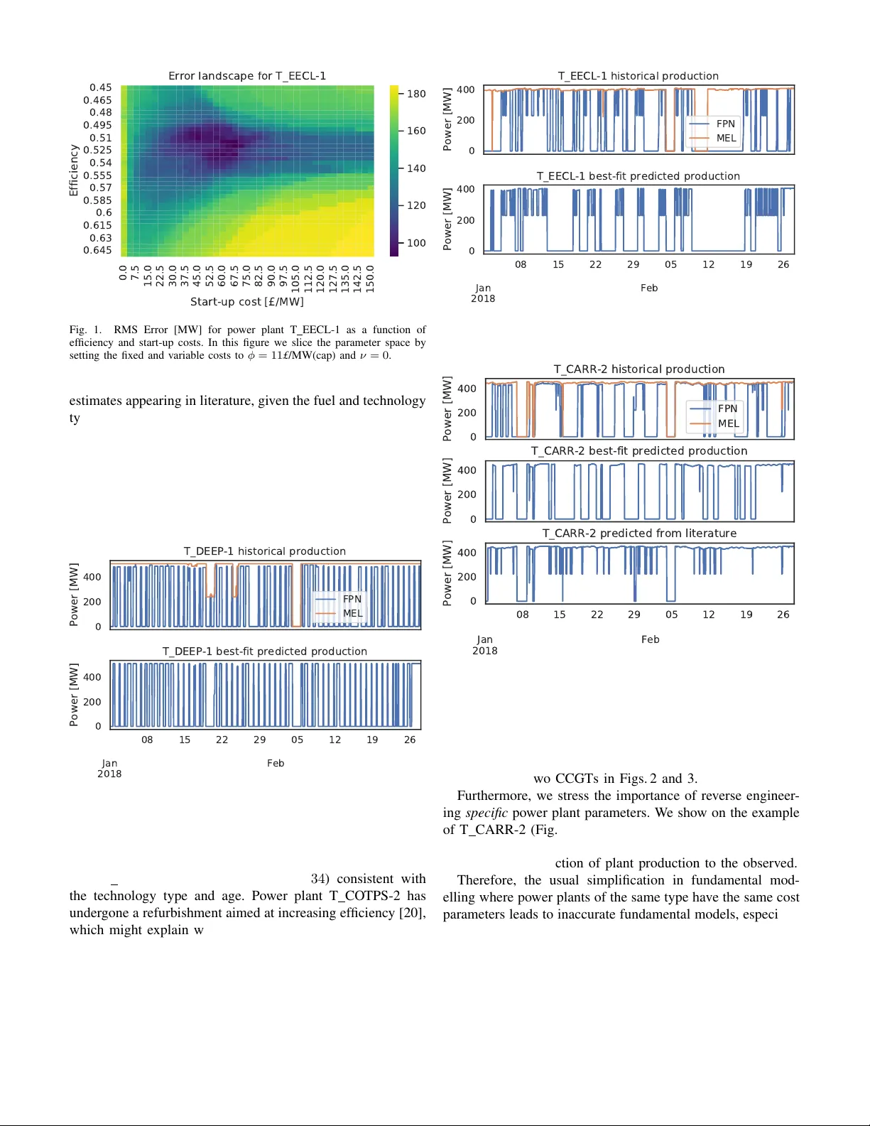
Extracting physical po wer plant parameters from historical beha viour David Kraljic, Miha T roha, Blaz Sobocan COMCOM d.o.o. Idrija, Slo venia Email: da vid.kraljic@comcom.si Abstract —The information needed for fundamental modelling of the power markets – the efficiency , start-up, fixed, and variable operating costs of each power plant – is not publicly a vailable. These parameters are usually estimated by considering the type of technology and the age of a power plant. W e present a method to extract these parameters for thermal power plants on the British electricity market using only the publicly available data. For each power plant, we solve a bilevel optimisation problem, wher e the inner level solv es the Unit Commitment (UC) problem and outputs the optimal schedule given the prices of fuel, emissions, electricity , and the unknown plant parameters. The outer level then optimises ov er the plant parameters matching the historical production of each plant as closely as possible. N O M E N C L A T U R E t T ime index dt T ime step between time indices [h] P t , P ∗ t , ˜ P t Power [MW] at time t : continuous v ariable, optimal solution of the UC, observed v alue P t Binary v ariable, one if power plant is on C t Binary variable, one if po wer plant has started m t Maximum Export Limit (MEL) [MW] r U P , r DN Ramping up and down limits [MW/h] η Thermal ef ficiency σ Start-up costs [ £ ] φ Fix ed O&M costs [ £ /h] ν V ariable O&M costs [ £ /MWh]  Emission factor [tCO 2 /MWh(fuel)] w t Wholesale electricity price [ £ /MWh] f t Fuel price [ £ /MWh(fuel)] e t Emissions price [ £ /tCO 2 ] I . I N T RO D U C T I O N The fundamental models of po wer markets are widely used, for example, to predict electricity prices or to answer ‘what- if ’ questions such as the ef fect of phasing out of nuclear power or increase in renewables. These models are easily interpreted, capture the non-linear dependence of the prices on demand, correctly incorporate the effect of changing fuel c  2019 IEEE. Personal use of this material is permitted. Permission from IEEE must be obtained for all other uses, in any current or future media, including reprinting/republishing this material for advertising or promotional purposes, creating new collecti ve works, for resale or redistribution to servers or lists, or reuse of any copyrighted component of this work in other works. and emission prices as well as intermittency of renew ables. These properties are the reason for wide use of fundamental models in the po wer markets, despite the spread of “machine learning” models in other fields. The key part of fundamental models is the supply curve (bid stack) - the supply of electricity ordered by the generators’ cost of production. The price in a competitiv e market then results from the equilibrium of the demand and the supply and equals the marginal cost of the last po wer plant needed to satisfy demand. The renewables, whose production cannot be controlled, and nuclear plants, whose production does not change significantly , are usually subtracted from the demand, such that the supply curve only needs to model thermal units. A good fundamental model, therefore, requires a detailed description of the thermal generators, which are usually modelled as a Unit Commitment problem [1]. The lack of information on exact physical and cost parameters of the generators, such as ef ficiency , start-up, fixed, and v ariable cost, results in simplified models. Generators are usually aggregated by fuel into a small number of units. Thermal ef ficiency is then estimated by considering the type of technology (e.g. simple cycle, combined cycle), fuel (e.g. coal, lignite, gas), and the age of power plants. Usually , only some of the cost types (fixed, v ariable, start-up) are considered and are assumed to be the same for plants of the same fuel type [2]–[4]. W e improv e on the current approaches of determining plant parameters, by presenting a method to reverse engineer the physical parameters of po wer plants such that the historical production is closely matched, based only on the publicly av ailable data. I I . D A TA W e consider large thermal units on the UK market for the year 2018. These units hav e to submit production plans to the system operator at least one hour in advance of deliv ery . This data represents what power plants have committed to generate and thus we take these submitted v olumes to represent po wer plants’ position on the wholesale market. These large units also hav e to submit some of their physical and dynamic data to the system operator, such as ramping rate limits, stable export limits, and maximum export limits. This data is taken as an input to our UC model. W e use the follo wing data sources: • Electricity prices: N2EX day-ahead auction [5] • Gas prices: ICE UK daily gas future [6] • Coal prices: UK major producers self-reported price [7] • Emission prices: EEX + UK Carbon Price Floor [8], [9] • Production: Production plans (FPN), ELEXON [10] • Export limits, ramping: Dynamic Data, ELEXON [10] • Emission factors [11] I I I . P RO B L E M D E S C R I P T I O N W e are interested in obtaining the physical and cost parame- ters (the efficienc y η , start-up costs σ , fixed operating costs φ , and v ariable operating costs ν ) that minimise the error between the historical production ˜ P t and the estimated production P ∗ t . The estimated production is obtained by solving the UC problem for the giv en physical and cost parameters. The described problem has a bilevel structure [12]: outer le vel: min η ,σ ,φ,ν X t  P ∗ t − ˜ P t  2 inner le vel: s. t. P ∗ t ∈ arg max UC, (1) where the inner UC optimisation problem is: max P t X t P t ( w t − ν − f t /η − e t /η ) dt − P t φ dt − C t σ s. t. C t +1 ≥ P t +1 − P t ∀ t − r DN ≤ P t +1 − P t ≤ r U P ∀ t P t ≤ m t P t ∀ t . . . (2) The first term in the UC objective represents the “clean spark spread”, the second term the fixed costs, and the third term the start-up costs. W e only list the most rele vant constraints. The actual formulation we use has sev eral additional constraints (and variables) modelling the fact that thermal power plants hav e a “Stable Export Limit” belo w which they cannot produce at a constant lev el b ut must be in a ramp up or do wn phase. A. Assumptions Our modelling relies on a couple of assumptions re garding the operational and market behaviour of real power plants: 1) Power plants run optimally by solving a UC problem of the form in Eq. 2. UC models might not capture the physical properties or business logic of power plans completely . For example, power plants might operate based on in-house developed heuristics instead of solving an optimisation problem, they might run less frequently to postpone maintenance, they might provide reserve services instead of participat- ing on the market, or they might take risks with respect to future or imbalance prices. 2) Power plants buy fuel, emissions and sell electricity on the spot market (i.e. day-ahead or intraday). Power plants can enter into long term contracts (e.g. sea- sonal, power purchasing agreements) for fuel, electricity , and emissions. Then they run such as to satisfy these obligations. The spot market assumption can be relaxed by including more market products for fuel, electricity etc. Howe ver , long term contracts are less transparent, therefore it is more dif ficult to estimate what prices the power plants get. B. Simplifications T aking the above assumptions as given, we also make certain simplifications in our UC modelling: 1) Efficienc y is independent of part-load 2) One ramping up (and do wn) rate across part-loads 3) Optimise once for whole year on day-ahead prices (i.e perfect price foresight) 4) One start-up cost (neglecting cold, warm, or more com- plicated start-up costs) 5) No minimum and maximum up and down times The UC modelling assumptions can all be mitigated by including extra complexity , with additional decision v ariables and constraints. Ho wev er , this comes at a cost. The underlying UC becomes more difficult to solv e and our bile vel problem becomes exponentially more difficult. For example, adding cold start-up costs adds two dimensions to our search space on the outer le vel, namely the time after which cold start-up costs apply and the v alue of the cold start-up cost. I V . S O LV I N G T H E B I L E V E L P RO B L E M The bilev el problem of Eqn. (1) can be solved by multiple methods. The simplest are direct search methods [13], such as compass search, brute force, and Nelder-Mead. The problem can also be solved with ev olutionary or swarm algorithms, such as differential e volution, particle sw arm, or simulated annealing [14]. The bilev el structure can also be transformed into a MILP [15], which is then solved with commercially av ailable solvers with the solution transformed back into the original bilevel problem at the end. W e have found that a combination of an ev olutionary algorithm [16] (to find an approximate location of minimum) followed by compass search works the f astest in practice as the computation can be massiv ely parallelised. The inner UC problem is a standard MILP we solve using Gurobi [17]. A. The err or landscape The objectiv e of the outer le vel is a function of plant parameters ( η , σ , φ , ν ). The solution of our bilev el problem is a minimum of this function. W e plot and illustrate this “error landscape” in Fig. 1. As the search space is four -dimensional we can only display 2D slices through the landscape. V . R E S U LT S A. Efficiencies In this section we sho w the ability of our approach to dis- cov er best-fit power plant parameters consistent with av erage 0.0 7.5 15.0 22.5 30.0 37.5 45.0 52.5 60.0 67.5 75.0 82.5 90.0 97.5 105.0 112.5 120.0 127.5 135.0 142.5 150.0 Start-up cost [£/MW] 0.45 0.465 0.48 0.495 0.51 0.525 0.54 0.555 0.57 0.585 0.6 0.615 0.63 0.645 Efficiency Error landscape for T_EECL-1 100 120 140 160 180 Fig. 1. RMS Error [MW] for po wer plant T EECL-1 as a function of efficienc y and start-up costs. In this figure we slice the parameter space by setting the fixed and variable costs to φ = 11 £ /MW(cap) and ν = 0 . estimates appearing in literature, given the fuel and technology type as well as the age of po wer plants. Figs. 2 and 3 are showing two CCGT power plants from late 1990s whereas Fig. 4 shows a CCGT built in 2016. The best- fit efficiencies are about 0.53 for the older plants and 0.58 for the newer , with start-up costs of about 50 £ /MW(cap), which is consistent with values for this type of technology and age group [2], [3], [18]. 0 200 400 Power [MW] T_DEEP-1 historical production FPN MEL Jan 2018 Feb 08 15 22 29 05 12 19 26 0 200 400 Power [MW] T_DEEP-1 best-fit predicted production Fig. 2. CCGT plant commissioned in 1994. Best-fit parameters are η = 0 . 53 , σ = 30 £ /MW(cap), φ = 9 . 0 £ /h/MW(cap), ν = 2 . 0 £ /MWh. Similarly , in Figs. 5 and 6 we present two coal power plants. Both were commissioned in the late 1960s. Howe ver , only T RA TS-1 has ef ficiency ( η = 0 . 34 ) consistent with the technology type and age. Power plant T CO TPS-2 has undergone a refurbishment aimed at increasing efficiency [20], which might explain why the best-fit ef ficiency ( η = 0 . 39 ) is higher than expected for this plant. B. Costs W e also sho w that po wer plants with the same efficiencies behav e very differently , depending on the structure of their 0 200 400 Power [MW] T_EECL-1 historical production FPN MEL Jan 2018 Feb 08 15 22 29 05 12 19 26 0 200 400 Power [MW] T_EECL-1 best-fit predicted production Fig. 3. CCGT plant commissioned in 1999. Best-fit parameters are η = 0 . 53 , σ = 55 £ /MW(cap), φ = 3 . 5 £ /h/MW(cap), ν = 6 . 5 £ /MWh. 0 200 400 Power [MW] T_CARR-2 historical production FPN MEL 0 200 400 Power [MW] T_CARR-2 best-fit predicted production Jan 2018 Feb 08 15 22 29 05 12 19 26 0 200 400 Power [MW] T_CARR-2 predicted from literature Fig. 4. CCGT plant commissioned in 2016. Best-fit parameters are η = 0 . 58 , σ = 62 £ /MW(cap), φ = 11 . 4 £ /h/MW(cap), ν = 0 . 9 £ /MWh. Literature parameters from [2], [3], [19] are η = 0 . 57 , σ = 24 £ /MW(cap), φ = 1 . 4 £ /h/MW(cap), ν = 2 . 4 £ /MWh. costs. For example, compare the very different production profiles of the two CCGTs in Figs. 2 and 3. Furthermore, we stress the importance of rev erse engineer - ing specific power plant parameters. W e show on the example of T CARR-2 (Fig. 4) that using the parameters appearing in the literature for this type and age of po wer plant leads to a very different prediction of plant production to the observed. Therefore, the usual simplification in fundamental mod- elling where po wer plants of the same type have the same cost parameters leads to inaccurate fundamental models, especially in the short term where electricity prices are often set by marginal costs of indi vidual po wer plants. V I . D I S C U S S I O N & C O N C L U S I O N W e have shown that our bile vel framework of reverse engineering power plant parameters is capable of describing 0 200 400 Power [MW] T_RATS-2 historical production FPN MEL Jan 2018 Feb 08 15 22 29 05 12 19 26 0 200 400 Power [MW] T_RATS-2 best-fit predicted production Fig. 5. Coal plant commissioned in 1969. Best-fit parameters are η = 0 . 34 , σ = 76 £ /MW(cap), φ = 4 . 8 £ /h/MW(cap), ν = 0 . 0 £ /MWh. 0 200 400 Power [MW] T_COTPS-2 historical production FPN MEL Jan 2018 Feb 08 15 22 29 05 12 19 26 0 200 400 Power [MW] T_COTPS-2 best-fit predicted production Fig. 6. Coal plant commissioned in 1969, refurbished 2014. Best-fit pa- rameters are η = 0 . 39 , σ = 30 £ /MW(cap), φ = 5 . 0 £ /h/MW(cap), ν = 2 . 0 £ /MWh. production profiles of real power plants. The obtained ef ficien- cies and start-up costs are consistent with the a verage estimates found in the literature. The inner model (UC) of our bilevel set-up can be replaced with any other model (e.g. a linear model, decision tree, neural network). Then our bile vel framework becomes a standard set- up of “machine learning”, where prediction error is minimised giv en some parametric model. Due to this similarity of our set- up and standard machine learning, the inner UC problem can be considered as an ef fective model of power plants, where the deduced parameters might not be the ones of the real power plants, but the ones that fit their beha viour best giv en the specific UC model and historical data. The advantages of using a UC model, besides interpretabil- ity , is that very complex behaviour can be specified with only a handful parameters (compared to hundreds in typical machine learning models) and there is no risk of overfitting the model. Howe ver , solving the UC problem and minimising the outer le vel error is computationally dif ficult, especially for more complex models (e.g. including minimum up/down times, se veral start-up costs, non-linear efficiency). This should be contrasted with e.g. linear models that have a closed-form solution, and fitting is performed in one step. The frame work we presented can be straightforwardly ex- tended. The UC model can be made more complex by in- cluding extra physical parameters describing the power plants. Instead of assuming perfect foresight on the market prices, we can run the inner UC model in sequence on shorter time frames, simulating real-time behaviour . Howe ver , all this comes at a large computational cost. R E F E R E N C E S [1] N. P . Padhy, “Unit commitment-a bibliographical surve y , ” IEEE T rans- actions on P ower Systems , vol. 19, no. 2, pp. 1196–1205, May 2004. [2] K. Bruninx, D. Madzharov , E. Delarue, and W . D’haeseleer , “Impact of the german nuclear phase-out on europe’ s electricity generationa comprehensiv e study , ” Ener gy P olicy , vol. 60, pp. 251 – 261, 2013. [Online]. A vailable: http://www .sciencedirect.com/science/article/ pii/S0301421513003583 [3] J. ˇ Sumbera and M. Dlouh ´ y, “ A model of german spot power market, ” Prague Economic P apers , vol. 2015, no. 3, pp. 287–306, 2015. [Online]. A vailable: https://EconPapers.repec.or g/RePEc:prg:jnlpep:v: 2015:y:2015:i:3:id:520:p:287- 306 [4] W .-P . Schill, M. Pahle, and C. Gambardella, “Start-up costs of thermal power plants in markets with increasing shares of variable rene wable generation, ” Natur e Ener gy , vol. 2, Apr 2017, 17050. [Online]. A vailable: https://doi.org/10.1038/nenergy .2017.50 [5] [Online]. A vailable: https://www .nordpoolgroup.com/Market- data1/GB/ Auction- prices/UK/ [6] [Online]. A vailable: https://www .theice.com/products/20774967/ UK- Natural- Gas- Daily- Future [7] [Online]. A vailable: https:// www .gov .uk/gov ernment/statistical- data- sets/ prices- of- fuels- purchased- by- major- po wer- producers [8] [Online]. A vailable: https://www .eex.com/en/ market- data/en vironmental- markets/deri vati ves- market/ european- emission- allow ances- futures [9] [Online]. A vailable: https://www .gov .uk/gov ernment/publications/ carbon- price- floor- reform [10] [Online]. A vailable: https://www .bmreports.com/bmrs/?q=balancing/ [11] K. Juhrich, “Co2 emission factors for fossil fu- els, ” Umweltbundesamt, T ech. Rep., Sep 2016. [On- line]. A vailable: https://www .umweltbundesamt.de/en/publikationen/ co2- emission- factors- for- fossil- fuels [12] A. Sinha, P . Malo, and K. Deb, “ A re view on bile vel optimization: From classical to e volutionary approaches and applications, ” IEEE T ransactions on Evolutionary Computation , vol. 22, no. 2, pp. 276–295, April 2018. [13] R. M. Lewis, V . T orczon, and M. W . T rosset, “Direct search methods: then and now , ” Journal of Computational and Applied Mathematics , vol. 124, no. 1, pp. 191 – 207, 2000, numerical Analysis 2000. V ol. IV : Optimization and Nonlinear Equations. [Online]. A vailable: http://www .sciencedirect.com/science/article/pii/S0377042700004234 [14] M. N. Ab W ahab, S. Nefti-Meziani, and A. Atyabi, “ A comprehensive revie w of swarm optimization algorithms, ” PLOS ONE , vol. 10, no. 5, pp. 1–36, 05 2015. [Online]. A vailable: https://doi.org/10.1371/journal. pone.0122827 [15] W . E. Hart, C. D. Laird, J.-P . W atson, D. L. W oodruf f, G. A. Hackebeil, B. L. Nicholson, and J. D. Siirola, Bilevel Pr ogramming . Cham: Springer International Publishing, 2017, pp. 223–233. [Online]. A vailable: https://doi.org/10.1007/978- 3- 319- 58821- 6 13 [16] R. Storn and K. Price, “Differential evolution – a simple and efficient heuristic for global optimization o ver continuous spaces, ” Journal of Global Optimization , vol. 11, no. 4, pp. 341–359, Dec 1997. [Online]. A vailable: https://doi.org/10.1023/A:1008202821328 [17] [Online]. A vailable: http://www .gurobi.com/ [18] J. Egerer , C. Gerbaulet, R. Ihlenburg, F . K unz, B. Reinhard, C. v on Hirschhausen, A. W eber, and J. W eibezahn, “Electricity Sector Data for Policy-Rele vant Modeling: Data Documentation and Applications to the German and European Electricity Markets, ” T ech. Rep., 2014. [19] R. T idball, J. Bluestein, N. Rodriguez, and S. Knoke, “Cost and performance assumptions for modeling electricity generation technologies, ” ICF International, Fairfax, V A, T ech. Rep. [Online]. A vailable: https://doi.org/10.2172/1219277 [20] [Online]. A vailable: https://www .theengineer.co.uk/ alstom- awarded- retrofit- contract/